Fermilab-Conf-96/329-T hep-ph/9610375 16 October 1996

Distinguishing Among Models of Strong ${\rm W}_{\rm L}{\rm W}_{\rm L}$ Scattering at the LHC
William B. Kilgore
Fermi National Accelerator Laboratory
P.O. Box 500
Batavia, IL 60510, USA

ABSTRACT

Using a multi-channel analysis of $W_{L}W_{L}$ scattering signals, I study the LHC’s ability to distinguish among various models of strongly interacting electroweak symmetry breaking sectors.

Abstract

Using a multi-channel analysis of $W_{L}W_{L}$ scattering signals, I study the LHC’s ability to distinguish among various models of strongly interacting electroweak symmetry breaking sectors.

1 Introduction

The most important question in particle physics today concerns the nature of the electroweak symmetry breaking mechanism. One of the most interesting and experimentally challenging possibilities is that the electroweak symmetry is broken by some new strong interaction. If this is the case, there may be no light quanta (of order a few hundred GeV or less), such as the Higgs boson, supersymmetric partners, etc., associated with the symmetry breaking sector. There will however be an identifiable signal of the symmetry breaking sector: strong $W_{L}W_{L}$ scattering.

The Goldstone boson equivalence theorem [1] states that at high energy, longitudinally polarized massive gauge bosons “remember” that they are the Goldstone bosons of the symmetry breaking sector. Accordingly, longitudinal gauge bosons in high energy scattering amplitudes can be replaced by the corresponding Goldstone bosons. For weakly interacting symmetry breaking sectors, this is merely a computational convenience. For strongly interacting symmetry breaking sectors, however, the equivalence theorem, coupled with the effective-W approximation [2] becomes a powerful tool for modeling high energy gauge boson scattering amplitudes.

Observing strong $W_{L}W_{L}$ scattering presents a very difficult experimental challenge. The scattering amplitudes grow with center of mass energy, but do not become large until the mass of the $W_{L}W_{L}$ system exceeds $\sim$1 TeV. At the LHC, the luminosity at such energies will be small and falling steeply, so that even though the scattering amplitudes are large, the cross section will be small, amounting to no more than tens of events per year. Nevertheless, it has been shown [3, 4, 5] that for all but a few pathological cases [6] the LHC will be able to establish the presence of strong $W_{L}W_{L}$ scattering, if it exists, in at least one scattering channel. It has also been shown that if strong $W_{L}W_{L}$ scattering is dominated by a single low-lying ($\sim$1 TeV) resonance, that resonance can be identified. The purpose of this study is to take a first look at the difficult task of distinguishing among different models of the symmetry breaking sector, even when there is not a single identifiable resonance. I will perform a multi-channel analysis on several different models of the symmetry breaking sector, comparing the predicted signals in each $W_{L}W_{L}$ scattering channel to those predicted by other models.

As the basis for this study, I will use the background calculations and signal identification cuts of Bagger et. al. [3], in which a standard set of cuts is identified for each scattering channel, and imposed consistently on the background processes and on a variety of models of strongly interacting symmetry breaking sectors.

2 $W_{L}W_{L}$ Scattering Channels

This analysis looks at $W_{L}W_{L}$ scattering into 5 different final states:

$ZZ\rightarrow\ell^{+}\ell^{-}\ell^{+}\ell^{-}$

$ZZ\rightarrow\ell^{+}\ell^{-}\nu\overline{\nu}$

$W^{\pm}Z\rightarrow\ell^{\pm}\nu\ell^{+}\ell^{-}$

$W^{+}W^{-}\rightarrow\ell^{+}\nu\ell^{-}\overline{\nu}$

$W^{\pm}W^{\pm}\rightarrow\ell^{\pm}\nu\ell^{\pm}\nu$ The $ZZ\rightarrow\ell^{+}\ell^{-}\nu\overline{\nu}$ is included because the small branching fraction of Z bosons into charged leptons severely limits the statistical significance of the $ZZ\rightarrow\ell^{+}\ell^{-}\ell^{+}\ell^{-}$ process.

In general, longitudinal $W_{L}$ pair production is dominated by the $W_{L}W_{L}$ fusion process, in which two incoming quarks radiate longitudinal $W_{L}$ bosons, which then rescatter off of one another as in Figure 1.

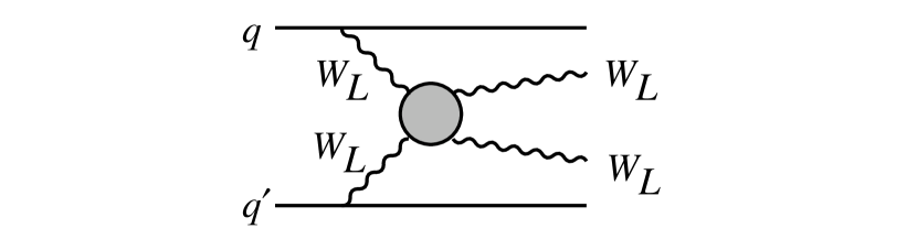
Figure 1: $W_{L}W_{L}$ Fusion process

Vector resonances also receive sizable contributions from $q\overline{q}^{\prime}$ annihilation into a gauge boson followed by mixing of the gauge boson into the vector resonance state, $q\overline{q}^{\prime}\rightarrow W^{*}\rightarrow\rho\rightarrow W_{L}W_{L}$.

The background in this study is taken to be the standard model with a light (100 GeV) Higgs boson. The signal for strong $W_{L}W_{L}$ scattering is an observable excess of gauge boson pairs over the expected rate from the standard model. The dominant background processes are $W_{L}W_{L}$ fusion into transverse W pairs ($qq\rightarrow qq^{\prime}W_{T}W_{T}(W_{T}W_{L})$), $q\overline{q}^{\prime}$ annihilation into W pairs plus jets, and top quark induced backgrounds.

The strongly interacting vector boson fusion process gives the signal events several distinctive characteristics which allow them to be distinguished from the background. The incoming quarks tend to emit longitudinal gauge bosons in the forward direction which then rescatter strongly off of one another. The forward emission tends to give the spectator quarks little recoil transverse momentum while the strong scattering process, which grows stronger with increasing center of mass energy, tends to be isotropic, throwing a large number of events into central rapidity regions. Thus, the signal is characterized by high invariant mass back-to-back gauge boson pairs accompanied by two forward jets from the spectator quarks and little central jet activity.

This is to be contrasted with the various background processes. $q\overline{q}^{\prime}$ annihilation tends to produce transversely polarized gauge bosons and no forward spectator jets. When jets are produced in association with $q\overline{q}^{\prime}$ annihilation, they often appear in central rapidities. Top induced backgrounds tend to produce very active events, characterized by jet activity in the vicinity of the gauge bosons. Perhaps the most dangerous background is the gauge boson fusion process producing at least one transversely polarized gauge boson since this process produces events with the same topology as the signal. Still, there are important differences. Interactions involving transversely polarized gauge bosons are weak (characterized by the weak gauge coupling) at all energies. In order for energetic gauge bosons to be thrown into the central region, they must typically recoil off of the emitting quarks, rather than off of one another. This hard recoil off of the quarks tends to throw the accompanying jets into the central region, rather than the forward.

These signatures can be used to help formulate a set of cuts which will enhance the signal at the expense of the background. One expects to find very energetic leptons in the central region of the detector. In addition, the leptons from one gauge boson tend to be back-to-back with those from the other gauge boson. In $ZZ$ modes, the invariant mass of the $ZZ$ pair tends to be large. In other modes, which cannot be fully reconstructed, the transverse mass of the gauge boson pair tends to be large. In addition, one can veto events with significant central jet activity, and tag for the forward spectator jets. The standard cuts used in Reference [3] are summarized in Table 1,

Table 1: Leptonic, single-jet-tagging and central-jet-vetoing cuts for generic $W_{L}W_{L}$ fusion processes at the LHC energy, by final-state mode.

$ZZ($4$\ell)$	Leptonic Cuts	Jet Cuts
	$|y({\ell})|<2.5$	$E_{tag}>0.8$ TeV
	$p_{T}(\ell)>40$ GeV	$3.0<|y_{tag}|<5.0$
	$p_{T}(Z)>p_{cm}(Z)/2$	$p_{T\ tag}>40$ GeV
	$M({ZZ})>500$ GeV	No Veto
$ZZ(\ell\ell\nu\nu)$	Leptonic Cuts	Jet Cuts
	$|y({\ell})|<2.5$	$E_{tag}>0.8$ TeV
	$p_{T}(\ell)>40$ GeV	$3.0<|y_{tag}|<5.0$
	$p_{T}^{\rm miss}>250$ GeV	$p_{T\ tag}>40$ GeV
	$M_{T}(ZZ)>500$ GeV	$p_{T\ veto}>60$ GeV
	$p_{T}{(\ell\ell)}>M_{T}(ZZ)/4$	$|y_{veto}|<3.0$
$W^{+}W^{-}$	Leptonic Cuts	Jet Cuts
	$|y({\ell})|<2.0$	$E_{tag}>0.8$ TeV
	$p_{T}(\ell)>100$ GeV	$3.0<|y_{tag}|<5.0$
	$\Delta p_{T}({\ell\ell})>440$ GeV	$p_{T\ tag}>40~{}$GeV
	$\cos\phi_{\ell\ell}<-0.8$	$p_{T\ veto}>30$ GeV
	$M({\ell\ell})>250$ GeV	$|y_{veto}|<3.0$
$W^{\pm}Z$	Leptonic Cuts	Jet Cuts
	$|y({\ell})|<2.5$	$E_{tag}>0.8$ TeV
	$p_{T}(\ell)>40$ GeV	$3.0<|y_{tag}|<5.0$
	$p_{T}^{\rm miss}>50$ GeV	$p_{T\ tag}>40$ GeV
	$p_{T}(Z)>{1\over 4}M_{T}(WZ)$	$p_{T\ veto}>60$ GeV
	$M_{T}(WZ)>500\ {\rm GeV}$	$|y_{veto}|<3.0$
$W^{\pm}W^{\pm}$	Leptonic Cuts	Jet Cuts
	$|y({\ell})|<2.0$
	$p_{T}(\ell)>70$ GeV	$3.0<|y_{tag}|<5.0$
	$\Delta p_{T}(\ell\ell)>200$ GeV	$p_{T\ tag}>40$ GeV
	$\cos\phi_{\ell\ell}<-0.8$	$p_{T\ veto}>60$ GeV
	$M(\ell\ell)>250$ GeV	$|y_{veto}|<3.0$

where $p_{cm}(Z)$ is the magnitude of the Z boson momentum in the diboson center of mass,

$$p_{cm}(Z)={1\over 2}\sqrt{M^{2}(ZZ)-4M_{Z}^{2}},$$ (1)

and the transverse masses are

$$M_{T}^{2}(ZZ) = \left[\sqrt{M_{Z}^{2}+p_{T}^{2}(\ell\ell)}+\sqrt{M_{Z}^{2}+|p_{T}^{\rm miss}|^{2}}\right]^{2}$$

$$-\left[{\vec{p}}_{T}(\ell\ell)+{\vec{p}}_{T}^{\rm miss}\right]^{2}$$

$$M_{T}^{2}(WZ) = \left[\sqrt{M^{2}(\ell\ell\ell)+p_{T}^{2}(\ell\ell\ell)}+|p_{T}^{\rm miss}|\right]^{2}$$

$$-\left[{\vec{p}}_{T}(\ell\ell\ell)+{\vec{p}}_{T}^{\rm miss}\right]^{2}.$$

The cuts in Table 1 are chosen to maximize the significance of each channel in the 1 TeV Higgs model. These cuts are not well suited for observing vector resonances in the $W^{\pm}Z$ channel. In the Higgs model, this channel, like all others, is dominated by the vector boson fusion process. The cuts therefore call for a forward jet tag. In vector resonance models, however, more than half of the signal in the $W^{\pm}Z$ channel comes from direct $q\overline{q}^{\prime}$ annihilation via mixing of the gauge boson and vector resonance states. Since these events are not accompanied by forward spectator jets, the jet tag cuts them out of the event sample. Reference [3] uses a special cut to enhance the $W^{\pm}Z$ signal in vector resonance models, but does not apply this cut to the other models.

3 Models

3.1 Formalism and the Lagrangian

Models of strongly interacting symmetry breaking sectors typically fall into one of three categories:

Nonresonant models.

Models with scalar resonances.

Models with vector resonances. Reference [3] describes eight different models of the symmetry breaking sector; three nonresonant models, three scalar resonance models, and two vector resonance models. The three nonresonant models differ in the unitarization procedures imposed upon them. The three scalar resonance models are the standard model with a 1 TeV Higgs boson, a nonlinearly realized chiral model with a 1 TeV scalar – isoscalar resonance (which differs from a Higgs boson by the strength of its coupling to the Goldstones), and an O(2N) symmetric scalar interaction. The vector resonance models incorporate vector – isovector resonances of masses 1 TeV and 2.5 TeV in a nonlinearly realized chiral symmetric interaction.

In this study I will use five of the models from Reference [3]: the K-matrix unitarized nonresonant model, the standard model, the chiral symmetric scalar resonance model and the vector resonance models. A single Lagrangian, transforming under a nonlinearly realized SU(2)${}_{L}\otimes$ SU(2)_R chiral symmetry, can be written down for all of these models, with particular couplings taking special values or set to zero as necessary. The Goldstone boson fields, $\pi^{a}$, are parameterized by the field

$$\xi=\exp{i{\sigma^{a}\pi^{a}\over 2v}},$$ (3)

where $\sigma^{a}$ are the Pauli matrices and $v$ is the electroweak vacuum expectation value. Under chiral rotations, $\xi$ transforms as

$$\xi\rightarrow\xi^{\prime}\equiv L\xi U^{\dagger}=U\xi R,$$ (4)

where L, R and U are elements of SU(2) and U is a nonlinear function of L, R and $\pi^{a}$.

With $\xi$ and its Hermitean conjugate $\xi^{\dagger}$, one can construct left- and right-handed currents,

$$J^{\mu}_{L} = \xi^{\dagger}\partial^{\mu}\xi\rightarrow UJ^{\mu}_{L}U^{\dagger}+U\partial^{\mu}U^{\dagger},$$

$$J^{\mu}_{R} = \xi\partial^{\mu}\xi^{\dagger}\rightarrow UJ^{\mu}_{R}U^{\dagger}+U\partial^{\mu}U^{\dagger}.$$

Note the inhomogeneous term $U\partial^{\mu}U^{\dagger}$, meaning that these currents transform as gauge fields under the diagonal $SU(2)$. From these chiral currents, one can form axial and vector currents,

$${\cal A}^{\mu} = J^{\mu}_{L}-J^{\mu}_{R}\rightarrow U{\cal A}^{\mu}_{L}U^{\dagger},$$

$$V^{\mu} = J^{\mu}_{L}+J^{\mu}_{R}\rightarrow UV^{\mu}U^{\dagger}+2U\partial^{\mu}U^{\dagger}.$$

The axial vector current transforms homogeneously under chiral transformation U but the vector current transforms inhomogeneously. This suggests that when we add the vector resonance $\rho_{\mu}=\rho_{\mu}^{a}\sigma^{a}/2$, it must transform as a gauge field under chiral transformations

$$\rho_{\mu}\rightarrow U\rho_{\mu}U^{\dagger}+i\tilde{g}^{-1}U\partial^{\mu}U^{\dagger}.$$ (7)

Now a new vector current can be formed which transforms homogeneously under chiral transformations,

$${\cal V}^{\mu}=V^{\mu}+2i\tilde{g}\rho^{\mu}\rightarrow U{\cal V}^{\mu}U^{\dagger}.$$ (8)

With these pieces and a scalar – isoscalar field $S$, we can construct the Lagrangian,

$${\cal L} = -{1\over 4}v^{2}{\rm Tr}{\cal A}^{\mu}{\cal A}_{\mu}-{a\over 4}v^{2}{\rm Tr}{\cal V}^{\mu}{\cal V}_{\mu}-{\lambda\over 2}vS{\rm Tr}{\cal A}^{\mu}{\cal A}_{\mu}$$

$$-{1\over 2}{\rm Tr}\rho_{\mu\nu}\rho^{\mu\nu}+{1\over 2}\partial^{\mu}S\partial_{\mu}S-{1\over 2}M^{2}_{S}S^{2}+\dots,$$

where $\rho^{a}_{\mu\nu}$ is the field strength tensor of the vector field $\rho^{a}_{\mu}$, and the ellipsis indicates higher derivative terms and other terms such as couplings between the scalar resonance and vector current which do not contribute to elastic $W_{L}W_{L}$ scattering.

In this notation, the resonances have masses and widths

$$M_{S}=M_{S} \Gamma_{S}={3\lambda^{2}M_{S}^{3}\over{32\pi v^{2}}}$$

$$M_{\rho}=a\tilde{g}^{2}v^{2} \Gamma_{\rho}={aM_{\rho}^{3}\over{192\pi v^{2}}}$$

Note that if $\lambda=1,a=0$, the scalar resonance $S$ is identical to an ordinary Higgs boson of the standard model. The Lagrangian in Equation 3.1 can thus parametrize a linear realization of $SU(2)_{L}\otimes SU(2)_{R}$ even though it is written in the language of non-linear realizations.

3.2 Details of Particular Models

In this analysis, I will use the results from the following models described in Reference [3].

The standard model with a 1.0 TeV Higgs boson ($\Gamma_{S}=$ 0.49 TeV). In the Lagrangian of Equation 3.1, this corresponds to setting $M_{S}=$ 1.0 TeV, $\lambda=$ 1, $a=$ 0.

A scalar resonance with $M_{S}=$ 1.0 TeV, $\Gamma_{S}=$ 0.35 TeV, corresponding to $\lambda=$ 0.84, $a=$ 0.

A vector resonance with $M_{\rho}=$ 1.0 TeV, $\Gamma_{\rho}=$ 0.0057 TeV, corresponding to $\lambda=$ 0, $a=$ 0.208, $\tilde{g}=$ 8.9.

A vector resonance with $M_{\rho}=$ 2.5 TeV, $\Gamma_{\rho}=$ 0.52 TeV, corresponding to $\lambda=$ 0, $a=$ 1.21, $\tilde{g}=$ 9.2.

A non-resonant model corresponding to $\lambda=$ 0, $a=$ 0. Note that the vector resonances considered are quite narrow. If one were to scale up QCD, vector resonances with masses of 1.0 and 2.5 TeV would have widths of 0.059 and 0.92 TeV respectively. The resonances in this study are taken to be so narrow in order to avoid constraints on the mixing of the Z boson with the resonance. These constraints come from the effect of the vector resonance on the spectral function of the Z boson. They could be relaxed if one were to assume, for instance, the presence of an axial vector resonance which would have a balancing effect on the spectral function, yet would not affect elastic $W_{L}W_{L}$ scattering [7].

4 Analysis

It has been well established [3, 4, 5] that the LHC will be able to demonstrate the existence or nonexistence of a strongly interacting electroweak symmetry breaking sector through direct observation of an excess of $W_{L}W_{L}$ events in at least one scattering channel. If such an excess is observed, one will want to understand what sort of interaction is responsible for the excess. Given the limited reach of the LHC into multi-TeV energies, a realistic goal is to try to fit the observed event rates in the various scattering channels to the predictions of various resonance models.

To that end, I take the predicted event rates (signal plus background) for each of the five models in turn, smear these rates by Poisson statistics and then compare the smeared results to the expectations of each model. By computing the mean chi-square with which the smeared “data” fits each model, I can determine the confidence level at which each model can be separated from the others.

In this study, I use the event rates for a single canonical LHC year of 100 ${\rm fb}^{\rm-1}$. One could argue that the LHC will run for several years and that the event rates should be multiplied by some factor such as 3 or 5. At present, however, I am concerned with what can be determined in a single year of running at design luminosity and will not speculate on the ultimate performance or lifetime of the LHC. The predicted event rates for the models are shown in Table 2.

Table 2: Event rates per 100 ${\rm fb}^{\rm-1}$ LHC year, assuming $\sqrt{s}=$ 14 TeV and $m_{t}=$ 175 GeV. Calculations were performed using the MRSA parton distribution set.

	$ZZ(4\ell)$	$ZZ(2\ell)$	$W^{+}W^{-}$	$W^{\pm}Z$	$W^{\pm}W^{\pm}$
Bkg.	0.7	1.8	12	4.9	3.7
SM	9	29	27	1.2	5.6
S 1.0	4.6	17	18	1.5	7.0
$\rho$ 1.0	1.4	4.7	6.2	4.5	12
$\rho$ 2.5	1.3	4.4	5.5	3.3	11
LET	1.4	4.5	4.6	3.0	13

Note again that the standard cuts for the $W^{\pm}Z$ channel given in Table 1 are not optimized for the detection of vector resonances since they cut out the half of the signal that comes from direct $q\overline{q}^{\prime}$ annihilation. Since the optimized cut is not applied to all models, I cannot use it for a quantitative analysis. I will however indicate its qualitative effect on the results below.

5 Results

The results of the analysis are presented in Table 3.

Table 3: Mean chi-square per degree of freedom for fitting the smeared “data” from each model to all of the models. The source of the “data” is indicated by the row. The model to which it is fit is indicated by the column.

	Higgs	Scalar	Vector	Vector	LET-K
	(1.0, 0.49)	(1.0, 0.35)	(1.0, 0.0057)	(2.5, 0.52)
Higgs
$M_{H}=$ 1.0 TeV	$\langle\chi^{2}\rangle=$ 0.82	$\langle\chi^{2}\rangle=$ 3.44	$\langle\chi^{2}\rangle=$ 26.3	$\langle\chi^{2}\rangle=$ 28.1	$\langle\chi^{2}\rangle=$ 28.1
$\Gamma_{H}=$ 0.49 TeV
Scalar
$M_{S}=$ 1.0 TeV	$\langle\chi^{2}\rangle=$ 2.17	$\langle\chi^{2}\rangle=$ 0.82	$\langle\chi^{2}\rangle=$ 7.74	$\langle\chi^{2}\rangle=$ 8.33	$\langle\chi^{2}\rangle=$ 8.56
$\Gamma_{S}=$ 0.35 TeV
Vector
$M_{\rho}=$ 1.0 TeV	$\langle\chi^{2}\rangle=$ 7.72	$\langle\chi^{2}\rangle=$ 3.75	$\langle\chi^{2}\rangle=$ 0.82	$\langle\chi^{2}\rangle=$ 0.93	$\langle\chi^{2}\rangle=$ 0.95
$\Gamma_{\rho}=$ 0.0057 TeV
Vector
$M_{\rho}=$ 2.5 TeV	$\langle\chi^{2}\rangle=$ 7.51	$\langle\chi^{2}\rangle=$ 3.59	$\langle\chi^{2}\rangle=$ 0.81	$\langle\chi^{2}\rangle=$ 0.82	$\langle\chi^{2}\rangle=$ 0.86
$\Gamma_{\rho}=$ 0.52 TeV
LET-K	$\langle\chi^{2}\rangle=$ 8.08	$\langle\chi^{2}\rangle=$ 3.99	$\langle\chi^{2}\rangle=$ 0.86	$\langle\chi^{2}\rangle=$ 0.90	$\langle\chi^{2}\rangle=$ 0.82

One can see that scalar resonance models are easily distinguished from vector resonance and non-resonant models. More surprising is that the 1.0 TeV Higgs boson is reasonably well separated from the narrower 1.0 TeV scalar resonance. The reason for this is that a Higgs theory is a renormalizable, unitary theory. The couplings of the gauge bosons to the Higgs cuts off the growth of the scattering amplitudes in all channels and unitarizes them. (Actually, tree level unitarity is violated when the Higgs is more massive than $\sim$800 GeV, but the theory is still renormalizable, and still unitary when higher order corrections are considered. The scalar resonance model is merely a low energy effective theory and is neither renormalizable nor unitary.) The smaller coupling of the narrower resonance to the gauge bosons is insufficient to unitarize the amplitudes.

The effect of this coupling strength is easily seen from Table 2. The amplitudes for $W^{+}W^{-}$ and $ZZ$ production are dominated by $s$-channel scalar exchange in the resonance region. The smaller coupling of the narrower resonance reduces the size of the signal in these channels. In $W^{\pm}Z$ and $W^{\pm}W^{\pm}$ production, t-channel scalar exchange reduces the magnitude of the scattering amplitudes. In these cases, the smaller coupling of the resonance causes the amplitudes to be reduced less than they would be by the Higgs, leading to larger signals.

Table 3 is somewhat misleading and overly pessimistic in that it indicates that vector resonance models cannot be distinguished from one another, nor from non-resonant models. This result is an artifact of the forward jet tag in the $W^{\pm}Z$ channel, which removes signal events due to $q\overline{q}^{\prime}$ annihilation. By eliminating the jet tag and looking in a window of transverse WZ mass surrounding the resonance, the 1.0 TeV vector state can be easily identified [3], and the model separated from the others with a high degree of confidence. The 2.5 TeV resonance, however, is too massive to be produced copiously, and cannot be distinguished from non-resonant strong scattering. Using considerably broader vector resonances, This conclusion is supported by References [4, 5], which have found that vector resonances can be clearly identified in the $W^{\pm}Z$ channel up to masses of 2.0 TeV, but that resonances above 2.5 TeV are difficult to distinguish from non-resonant strong scattering.

6 Discussion

There are many ways in which this analysis can be improved. One of the most obvious improvements would be in the choice of cuts. This analysis applies the same basic set of cuts, optimized for the 1 TeV Higgs signal, to all models. This strategy serves the purpose for which it was intended by setting a standard by which one can tell if strong $W_{L}W_{L}$ scattering is occurring, but it is not well suited to the present analysis which attempts to distinguish among models of strong scattering. In particular, since the $W^{\pm}Z$ signal in a Higgs model is optimized by using forward jet tags, the cuts remove much of the $W^{\pm}Z$ signal that occurs in a vector resonance model. A better analysis would optimize the cuts in each scattering channel for each model. One would then need to compute the performance of each model under the other models’ optimized cuts. Given a set of cuts, one can easily compute the performance of the various models. The difficulty lies in performing the optimization. The detailed background investigations that would be required are beyond the scope of this study.

This study would also be improved by adding more models. It would be interesting to determine the reach for identifying vector resonances more precisely. It would also be interesting to look at models with both scalar and vector resonances and study how their signal patterns interfere with one another.

Yet another improvement on this study would be to move beyond its reliance on gold plated purely leptonic modes. The ATLAS and CMS collaborations have both studied searches for 1 TeV Higgs bosons decaying via “silver plated” modes, in which one gauge boson decays leptonically while the other decays into jets, with positive results [8, 9]. The benefit of using the silver plated modes is that the hadronic branching fraction is much larger than the leptonic branching fraction, providing a sizable increase in rate. On the other hand, the hadronic decay modes are much messier and depend much more sensitively on the details of calorimetric performance. In addition, one cannot determine the charge of the hadronically decaying gauge boson, obscuring the clean separation of scattering channels. A full investigation of the detection of silver plated modes must await a better understanding of the actual detectors, and will be best performed by the experimental collaborations themselves.

7 Conclusions

The LHC will be able to establish the presence or absence of strong $W_{L}W_{L}$ for most models of the strongly interacting symmetry breaking sector. Making use of all $W_{L}W_{L}$ scattering channels, this analysis shows that the LHC will not only be able to identify low lying resonances, but will also be able to distinguish among different resonance models. In the few models studied here, it is apparent that resonances near 1 TeV can be readily identified but that models with resonances above 2.5 TeV are indistinguishable from non-resonant models. A more definite limit on resonance identification and ultimately on the LHC’s ability to distinguish among strong scattering models requires a more complete analysis along the lines detailed above.

8 Acknowledgments

I would like to thank Persis Drell and Sekhar Chivukula for helpful comments during this analysis. Fermilab is operated by Universities Research Association, Inc., under contract DE-AC02-76CH03000 with the U.S. Department of Energy.

References

-
[1]
J.M. Cornwall, D.N. Levin, and G. Tiktopoulos, Phys. Rev. D 10 (1974) 1145;
C.E. Vayonakis, Lett. Nuovo Cim. 17 (1976) 383;
B.W. Lee, C. Quigg, and H. Thacker, Phys. Rev. D 16 (1977) 1519;
M.S. Chanowitz and M.K. Gaillard, Nucl. Phys. B 261 (1985) 379. -
[2]
M.S. Chanowitz and M.K. Gaillard, Phys. Lett. B
142 (1984) 85;
G. Kane, W. Repko, B. Rolnick, Phys. Lett. B 148 (1984) 367;
S. Dawson, Nucl. Phys. B 29 (1985) 42. - [3] J. Bagger, et al, Phys. Rev. D 52 (1995) 3878. (hep-ph/9504426)
- [4] M.S. Chanowitz and W.B. Kilgore, Phys. Lett. B 322 (1994) 147. (hep-ph/9412275)
- [5] M.S. Chanowitz and W.B. Kilgore, Phys. Lett. B 347 (1995) 387. (hep-ph/9311336)
-
[6]
R.S. Chivukula and M. Golden, Phys. Lett B 267 (1991) 233;
T. Binoth and J.J. van der Bij, FREIBURG-THEP-96-04 (1996). (hep-ph/9603427);
T. Binoth and J.J. van der Bij, FREIBURG-THEP-96-15 (1996). (hep-ph/9608245) -
[7]
M.E. Peskin and T. Takeuchi, Phys. Rev. Lett. 65 (1990) 964;
Phys. Rev. D 46 (1991) 381. - [8] ATLAS Collaboration, Technical Proposal, CERN/LHCC 94-43 .
- [9] CMS Collaboration, Technical Proposal, CERN/LHCC 94-38.