FTUV/96-69

IFIC/96-78

NORDITA-96/70 N,P

hep-ph/9610360

Revised

Electromagnetic Corrections for Pions and Kaons : Masses and Polarizabilities
Johan Bijnens^a and Joaquim Prades^b
a NORDITA, Blegdamsvej 17,

DK-2100 Copenhagen Ø, Denmark

^b Departament de Física Teòrica, Universitat de València

and IFIC, CSIC - Universitat de València, C/ del Dr. Moliner 50, E-46100 Burjassot (València) Spain

The unknown constants in Chiral Perturbation Theory needed for an all orders analysis of the polarizabilities and electromagnetic corrections to the masses of the pseudo-Goldstone bosons are estimated at leading order in $1/N_{c}$. We organize the calculation in an $1/N_{c}$-expansion and separate long- and short-distance physics contributions by introducing an Euclidean cut-off. The long-distance part is evaluated using the ENJL model and the short-distance part using perturbative QCD and factorization. We obtain very good matching between both.

We then include these estimates in a full Chiral Perturbation Theory calculation to order $e^{2}$ $p^{2}$ for the masses and $p^{6}$ for the polarizabilities. For the electromagnetic corrections to the masses, we confirm a large violation of Dashen’s theorem getting a more precise value for this violation. We make comparison with earlier related work. Some phenomenological consequences are discussed too.

PACS numbers: 13.40.Dk, 13.40Gp, 13.40.Ks, 14.40.Aq, 11.15.Pg, 12.39.Fe
Keywords: Pion, Kaon, Electromagnetic Mass, Polarizabilities October 1996

1 Introduction

Virtual electromagnetic (EM) effects in purely strong processes can be important in precision situations. This is especially true in the case of isospin breaking contributions to hadron masses and some hadronic processes. If we want a high precision description of the latter, we need to know not only the effects due to the quark mass difference $m_{d}-m_{u}$, which is a quantity we would also like to extract from these experiments, but the size of the electromagnetic contributions.

That these contributions can be sizeable in certain cases is best illustrated in the case of the observed $\pi^{+}-\pi^{0}$ mass difference which is almost entirely due to photon loops [2]. At present, we cannot directly use QCD to estimate these effects. Some first progress using lattice QCD has been made recently in [3]. Instead we turn to the method of Chiral Perturbation Theory (CHPT). In the purely mesonic sector for the strong and semi-leptonic processes, this was started as a systematic program by Gasser and Leutwyler [4, 5] and has since then been extended to a large variety of processes[6]. In the case of $\gamma\gamma\to\pi\pi$[7, 8], $\pi\pi$-scattering [9] and $\pi\to\ell\nu\gamma$ [10] this has even been done to the two-loop order. In $\pi\pi$-scattering, electromagnetic corrections might also become relevant at the precision achieved by the two-loop order calculation. They are already important, at the present level of precision, in various others form factors.

Chiral Perturbation Theory for virtual electromagnetic effects was first described at lowest order ($e^{2}p^{0}$) in [11]. Urech[12] has recently systematically studied the next-to-leading order terms. His work has been mainly dedicated to the EM correction in the masses of the lowest pseudoscalar Goldstone bosons. This program has been later expanded into a few more form factors by Neufeld and Rupertsberger[13, 14]. The results were, however, quite dependent on the values for the new coupling constants appearing at order $e^{2}$ $p^{2}$ in the chiral expansion. Unfortunately, contrary to the case of strong and semileptonic processes, it is impossible to determine all these constants from experimental data. The calculation of these constants is the main subject of this paper. In addition we provide estimates for the counterterms appearing in CHPT at order $p^{6}$ in the processes $\gamma\gamma\to PP$. Here we extend the work done in [15] to the charged case and make predictions for the polarizabilities of pions and kaons too. This side aspect is discussed in Section 7.

The real problem in calculating the constants is that it requires an integration over internal photon momenta. For instance, in the estimate done for the strong sector in [16] using the lowest lying resonance saturation, only their lowest order couplings are relevant. When one integrates over all photon momenta, the couplings of the resonances to all orders need to be known, thus making these estimates much more difficult. The lowest order constant, called $C$ in Section 2, has a very long history, it was first estimated in [2] using PCAC and then saturating two-point functions with resonance exchanges. A different technique was subsequently developed by Bardeen, Buras and Gérard in [17] for weak non-leptonic matrix elements, now generally referred to as the $1/N_{c}$-approach. This approach was then used together with the Das et al. sum rule [2] to estimate the pion mass difference at lowest order, or equivalently $C$, in [18]. Here a proper separation of long and short distance contributions was also possible. The same method has been used in the chiral quark model[19] and in the extended Nambu–Jona-Lasinio (ENJL) model[20]. All of these only allowed estimates of the lowest order constant $C$ since they were based on the Das et al. sum rule.

The calculation of the pion and kaon EM mass differences beyond lowest order in CHPT, using saturation by the lowest lying resonances, was recently performed by Donoghue, Holstein, and Wyler in [21] and Baur and Urech in [22]. For earlier attempts see [23]. In [24] the chiral logs at $\nu=1$ GeV were used to estimate these EM mass differences. These papers all had to make assumptions about the short distance behaviour. More comments about these assumptions are in Section 5. The short-distance contribution was introduced in an operator-product expansion (OPE) framework in [25]. This is discussed in Section 3.1.

The method used in this paper is an extension of the original $1/N_{c}$ method[17]. We use an off-shell Green function. This method was used by us previously in the calculation of the $\Delta S=2$ hadronic matrix element in the $K^{0}$-$\overline{K^{0}}$ system and commonly parametrized by the so-called $B_{K}$ factor [26].

The paper is organized as follows: in Section 2 we shortly discuss CHPT for electromagnetic corrections and define our set of counterterms. Our set is somewhat more appropriate to the large $N_{c}$ limit and different number of flavours. We also point out in some detail the gauge dependence of the generating functional. No observable quantities do of course depend on the gauge but the infinite parts of the constants at next-to-leading order do depend on it. In Section 3 we explain the method. This section also gives a short overview of the ENJL model that we use for the long-distance contributions. The main contributions are the latter due to the photon propagator. In Section 4 we give the results and use CHPT at leading order in $1/N_{c}$ to extract the CHPT constants. We compare with the earlier work in Section 5. Section 6 summarizes the consequences for the ratios of the light current quark masses. Section 7 contains the results on pion and kaon polarizabilities and we present our main conclusions in Section 8.

2 Chiral Perturbation Theory Analysis

In this Section we use CHPT to analyse the two-point functions,

$${}\Pi(q^{2})=i{\displaystyle\int}\,{\rm d}^{4}x\,e^{iqx}\,\langle 0|T\left(P(0)P^{\dagger}(x)\right)|0\rangle\,,$$ (2.1)

in the presence of electromagnetic interactions. We shall do this to first order in $\alpha_{QED}$ and to order $p^{2}$ in CHPT. The pseudoscalar source $P(x)$ in (2.1) is defined as $\left(\overline{q}_{a}i\gamma_{5}q_{b}\right)(x)$, with $a$, $b$ quark flavour indices and colour indices summed inside the parenthesis.

At lowest order in the chiral expansion ${\cal O}(p^{2})$ [27], the strong interactions between the lowest pseudoscalar mesons including external vector, axial-vector, scalar and pseudoscalar sources are described by the following effective Lagrangian

$${}{\cal L}^{(2)}_{\rm eff} = \frac{\displaystyle F_{0}^{2}}{\displaystyle 4}\left\{\mathrm{tr}\left(D_{\mu}UD^{\mu}U^{\dagger}\right)+\mathrm{tr}\left(\chi U^{\dagger}+U\chi^{\dagger}\right)\right\}$$ (2.2)

where $D_{\mu}$ denotes the covariant derivative

$${}D_{\mu}U=\partial_{\mu}U-i(v_{\mu}+a_{\mu})U+iU(v_{\mu}-a_{\mu}),$$ (2.3)

and $U\equiv{\rm exp}\left(\frac{\displaystyle i\sqrt{2}\Phi}{\displaystyle F_{0}}\right)$ an SU(3) matrix incorporating the octet of pseudoscalar mesons

$${}\Phi(x)=\frac{\vec{\lambda}}{\sqrt{2}}\vec{\phi}=\left(\begin{array}[]{ccc}\frac{\displaystyle\pi^{0}}{\displaystyle\sqrt{2}}+\frac{\displaystyle\eta_{8}}{\displaystyle\sqrt{6}}&\pi^{+}&K^{+}\\ \pi^{-}&-\frac{\displaystyle\pi^{0}}{\displaystyle\sqrt{2}}+\frac{\displaystyle\eta_{8}}{\displaystyle\sqrt{6}}&K^{0}\\ K^{-}&\overline{K}^{0}&-\frac{\displaystyle 2\eta_{8}}{\displaystyle\sqrt{6}}\end{array}\right)\,.$$ (2.4)

In Eq. (2.3), $v_{\mu}(x)$ and $a_{\mu}(x)$ are external 3 $\times$ 3 vector and axial-vector field matrices. When electromagnetism is switched on, $v_{\mu}(x)=|e|QA_{\mu}(x)$ and $a_{\mu}(x)=0$. Here $A_{\mu}(x)$ is the photon field and the light-quark electric charges in units of the electron charge $|e|$ are collected in the 3 $\times$ 3 flavour matrix $Q=\frac{1}{3}{\rm diag}(2,-1,-1)$. In Eq. (2.2) $\chi\equiv 2B_{0}({\cal M}+s(x)+ip(x))$ with $s(x)$ and $p(x)$ external scalar and pseudoscalar 3 $\times$ 3 field matrices and ${\cal M}$ the 3 $\times$ 3 flavour matrix ${\cal M}={\rm diag}(m_{u},m_{d},m_{s})$ collecting the light-quark current masses. The constant $B_{0}$ is related to the vacuum expectation value

$$\left.\langle 0|\bar{q}q|0\rangle\right|_{q=u,d,s}=-F_{0}^{2}B_{0}\left(1+{\cal O}(m_{q})\right)\,.$$ (2.5)

In this normalization, $F_{0}$ is the chiral limit value corresponding to the pion decay coupling $F_{\pi}\simeq 92.4$ MeV. In the absence of the U(1)_A anomaly (large $N_{c}$ limit) [28], the SU(3) singlet $\eta_{1}$ field becomes the ninth Goldstone boson which is incorporated in the $\Phi(x)$ field as

$${}\Phi(x)=\frac{\vec{\lambda}}{\sqrt{2}}\vec{\phi}+\frac{\eta_{1}}{\sqrt{3}}{\mbox{\large\bf 1}}\,.$$ (2.6)

To this order, the two-point functions in (2.1) have the following form

$${}\Pi(q^{2})=-\frac{2B_{0}^{2}F_{0}^{2}}{q^{2}-m_{0}^{2}},$$ (2.7)

where $m_{0}$ is the pseudo-Goldstone boson masses to that order, i.e. $m_{0}^{2}=B_{0}(m_{a}+m_{b})$, with $m_{a}$ the flavour $a$ quark mass. Here we are interested in the isospin breaking corrections to the poles of these two-point functions induced by electromagnetism to order $e^{2}$. So we will set $m_{u}=m_{d}$ in the calculation.

To take into account virtual photons excitations we need to add to the Lagrangian in (2.2) the corresponding kinetic and gauge fixing terms, i.e.

$${}-\frac{1}{4}F^{\mu\nu}F_{\mu\nu}-\frac{1}{2(1-\xi)}\,\left(\partial_{\mu}A^{\mu}\right)^{2}$$ (2.8)

where $F^{\mu\nu}=\partial^{\mu}A^{\nu}-\partial^{\nu}A^{\mu}$ is the electromagnetic field strength tensor. The parameter $\xi$ is the gauge fixing parameter which is zero in the Feynman gauge, one in the Landau gauge and four in Yennie’s one.

2.1 Lowest Order Contribution

At lowest order in the chiral expansion, electromagnetic (EM) virtual interactions of order $e^{2}$ between the pseudo-Goldstone bosons are described by the following effective Lagrangian [5, 28, 29]

$${}{\cal L}^{(0)}_{e^{2}} = e^{2}C_{1}(\Phi_{0}^{2})\mathrm{tr}\left(Q^{2}\right)+e^{2}C_{2}(\Phi_{0}^{2})\mathrm{tr}\left(QUQU^{\dagger}\right).$$ (2.9)

Here the $U$ field matrix is the U(3) symmetric one in (2.6) and $\Phi_{0}=\theta+\eta_{1}\sqrt{6}/F_{0}$, where $\theta$ is the so-called QCD theta-vacuum parameter. The constant $C=C_{2}(0)$ is the coupling introduced in [16]. There are no loop contributions to this order and therefore $C_{1,2}(0)$ and the derivatives of $C_{1,2}(x)$ at $x=0$ are finite counterterms not fixed by symmetry alone. In the large $N_{c}$ limit, $C_{1,2}(0)$ are of order $N_{c}$ whereas the $n$-th derivative of $C_{1,2}(x)$ is of order $1/N_{c}^{2n-1}$. To order $e^{2}p^{0}$, the correction to the pole position of the two-point function in (2.7) is zero for $P=\pi^{0}$ and $P=\eta_{8}$, while charged pion and kaons get the same non-zero correction, namely

$$m^{2}_{\em EM(\pi^{+},K^{+})}=e^{2}\,\frac{2C}{F_{0}^{2}}.$$ (2.10)

This is the so-called Dashen’s theorem [11]. The pole position for the $\eta_{1}$-$\eta_{1}$ two-point function gets corrected by

$$m^{2}_{\em EM(\eta_{1})}=e^{2}\,\frac{8(C^{\prime}_{1}(0)+C^{\prime}_{2}(0))}{F_{0}^{2}}$$ (2.11)

from EM virtual interactions.

2.2 Next-to-Leading Order Contribution

In this Section we shall report on the CHPT order $p^{2}$ $e^{2}$ virtual EM corrections. The first type of these corrections is the emission and absorption of a photon by a pseudo-Goldstone boson line (see Fig. 1). To the order we are interested here, the $\gamma P^{+}P^{-}$ and $\gamma\gamma P^{+}P^{-}$ vertices come from the Lagrangian in (2.2). This contribution needs a counterterm of order $e^{2}p^{2}$ to make it UV finite.

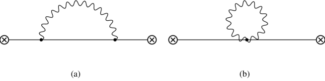
Figure 1: The photon loop contributions to (3.1). The crosses are pseudoscalar currents. The wiggly line is the photon. The full lines are pseudoscalars.

The complete CHPT order $p^{2}$ effective Lagrangian describing virtual EM interactions of order $e^{2}$ between pseudo-Goldstone bosons and external vector, axial-vector, scalar and pseudoscalar sources was written in [12] (see also [14]). The coefficients of this Lagrangian are the needed counterterms to absorb the UV divergences of order $e^{2}p^{2}$. To construct this Lagrangian, some Cayley-Hamilton relations for SU(3) matrices were used. We would like here to include also the ninth pseudo-Goldstone boson as above and work with U(3) matrices (see Eq. (2.6)), which is the symmetry in the large $N_{c}$ limit ($N_{c}$ is the number of colours). This is useful for our calculation since we want to use the $1/N_{c}$-expansion as the organizing scheme. To order $e^{2}p^{2}$, one has to add to the Lagrangians in (2.2), (2.8), and (2.9) the following one:

$${}{\cal L}^{(2)}_{e^{2}} = e^{2}\tilde{K}_{1}(\Phi_{0}^{2})F_{0}^{2}\,\mathrm{tr}\left(D^{\mu}U^{\dagger}D_{\mu}U\right)\mathrm{tr}\left(Q^{2}\right)$$

$$+ e^{2}\tilde{K}_{2}(\Phi_{0}^{2})F_{0}^{2}\,\mathrm{tr}\left(D^{\mu}U^{\dagger}D_{\mu}U\right)\mathrm{tr}\left(QUQU^{\dagger}\right)$$

$$+ e^{2}\tilde{K}_{3}(\Phi_{0}^{2})F_{0}^{2}\,\mathrm{tr}\left(QU^{\dagger}D^{\mu}UQD_{\mu}U^{\dagger}U+QUD^{\mu}U^{\dagger}QD_{\mu}UU^{\dagger}\right)$$

$$+ e^{2}\tilde{K}_{4}(\Phi_{0}^{2})F_{0}^{2}\,\mathrm{tr}\left(QU^{\dagger}D^{\mu}UQD_{\mu}UU^{\dagger}\right)$$

$$+ e^{2}\tilde{K}_{5}(\Phi_{0}^{2})F_{0}^{2}\,\mathrm{tr}\left(\left(D^{\mu}U^{\dagger}D_{\mu}U+D^{\mu}UD_{\mu}U^{\dagger}\right)Q^{2}\right)$$

$$+ e^{2}\tilde{K}_{6}(\Phi_{0}^{2})F_{0}^{2}\,\mathrm{tr}\left(D^{\mu}U^{\dagger}D_{\mu}UQU^{\dagger}QU+D^{\mu}UD_{\mu}U^{\dagger}QUQU^{\dagger}\right)$$

$$+ e^{2}K_{7}(\Phi_{0}^{2})F_{0}^{2}\,\mathrm{tr}\left(\chi^{\dagger}U+U^{\dagger}\chi\right)\mathrm{tr}\left(Q^{2}\right)$$

$$+ e^{2}K_{8}(\Phi_{0}^{2})F_{0}^{2}\,\mathrm{tr}\left(\chi^{\dagger}U+U^{\dagger}\chi\right)\mathrm{tr}\left(QUQU^{\dagger}\right)$$

$$+ e^{2}K_{9}(\Phi_{0}^{2})F_{0}^{2}\,\mathrm{tr}\left(\left(\chi^{\dagger}U+U^{\dagger}\chi+\chi U^{\dagger}+U\chi^{\dagger}\right)Q^{2}\right)$$

$$+ e^{2}K_{10}(\Phi_{0}^{2})F_{0}^{2}\,\mathrm{tr}\left(\left(\chi^{\dagger}U+U^{\dagger}\chi\right)QU^{\dagger}QU+\left(\chi U^{\dagger}+U\chi^{\dagger}\right)QUQU^{\dagger}\right)$$

$$+ e^{2}K_{11}(\Phi_{0}^{2})F_{0}^{2}\,\mathrm{tr}\left(\left(\chi^{\dagger}U-U^{\dagger}\chi\right)QU^{\dagger}QU+\left(\chi U^{\dagger}-U\chi^{\dagger}\right)QUQU^{\dagger}\right)$$

$$+ e^{2}K_{12}(\Phi_{0}^{2})F_{0}^{2}\,\mathrm{tr}\left(UD^{\mu}U^{\dagger}\left[\nabla^{R}_{\mu}Q,Q\right]\,+\,U^{\dagger}D^{\mu}U\left[\nabla^{L}_{\mu}Q,Q\right]\right)$$

$$+ e^{2}K_{13}(\Phi_{0}^{2})F_{0}^{2}\,\mathrm{tr}\left(\nabla^{R}_{\mu}QU\nabla_{L}^{\mu}QU^{\dagger}\right)$$

$$+ e^{2}K_{14}(\Phi_{0}^{2})F_{0}^{2}\,\mathrm{tr}\left(\nabla^{R}_{\mu}Q\nabla_{R}^{\mu}Q+\nabla^{L}_{\mu}Q\nabla_{L}^{\mu}Q\right)$$

$$+ e^{2}\tilde{K}_{15}(\Phi_{0}^{2})F_{0}^{2}\mathrm{tr}\left(\left(D_{\mu}UU^{\dagger}-D_{\mu}U^{\dagger}U\right)Q^{2}\right)\,\delta^{\mu}\theta$$

$$+ e^{2}\tilde{K}_{16}(\Phi_{0}^{2})F_{0}^{2}\mathrm{tr}\left(D_{\mu}UQU^{\dagger}Q-D_{\mu}^{\dagger}QUQ\right)\,\delta^{\mu}\theta$$

$$+ e^{2}\tilde{K}_{17}(\Phi_{0}^{2})F_{0}^{2}\left(\mathrm{tr}\left(Q^{2}\right)\,+\,\mathrm{tr}\left(QUQU^{\dagger}\right)\right)\,D^{\mu}\Phi_{0}D_{\mu}\Phi_{0}$$

$$+ e^{2}\tilde{K}_{18}(\Phi_{0}^{2})F_{0}^{2}\left(\mathrm{tr}\left(Q^{2}\right)\,+\,\mathrm{tr}\left(QUQU^{\dagger}\right)\right)\,D^{\mu}\Phi_{0}\delta_{\mu}\theta$$

$$+ e^{2}\tilde{K}_{19}(\Phi_{0}^{2})F_{0}^{2}\left(\mathrm{tr}\left(Q^{2}\right)\,+\,\mathrm{tr}\left(QUQU^{\dagger}\right)\right)\,\delta^{\mu}\theta\delta_{\mu}\theta$$

$$+ e^{2}\Phi_{0}\tilde{K}_{20}(\Phi_{0}^{2})F_{0}^{2}\mathrm{tr}\left(\chi^{\dagger}U-U^{\dagger}\chi\right)\mathrm{tr}\left(Q^{2}\right)$$

$$+ e^{2}\Phi_{0}\tilde{K}_{21}(\Phi_{0}^{2})F_{0}^{2}\mathrm{tr}\left(\chi^{\dagger}U-U^{\dagger}\chi\right)\mathrm{tr}\left(QUQU^{\dagger}\right)$$

$$+ e^{2}\Phi_{0}\tilde{K}_{22}(\Phi_{0}^{2})F_{0}^{2}\mathrm{tr}\left(\left(U\chi^{\dagger}+\chi^{\dagger}U-U^{\dagger}\chi-\chi U^{\dagger}\right)Q^{2}\right)$$

$$+ e^{2}\Phi_{0}\tilde{K}_{23}(\Phi_{0}^{2})F_{0}^{2}\mathrm{tr}\left(\left(\chi^{\dagger}U+U^{\dagger}\chi\right)QU^{\dagger}QU-\left(\chi U^{\dagger}+U^{\dagger}\chi\right)QUQU^{\dagger}\right)$$

$$+ e^{2}\Phi_{0}\tilde{K}_{24}(\Phi_{0}^{2})F_{0}^{2}\mathrm{tr}\left(\left(\chi^{\dagger}U-U^{\dagger}\chi\right)QU^{\dagger}QU-\left(\chi U^{\dagger}-U\chi^{\dagger}\right)QUQU^{\dagger}\right)$$

It is interesting to study the large $N_{c}$ behaviour of the coefficients in (2.2). In the large $N_{c}$ limit, the couplings $\tilde{K}_{1}(0)$, $\tilde{K}_{2}(0)$, $K_{7}(0)$, $K_{8}(0)$, $\tilde{K}_{15}(0)$, $\tilde{K}_{16}(0)$, $\tilde{K}_{22}(0)$, $\tilde{K}_{23}(0)$, and $\tilde{K}_{24}(0)$ are order $1/N_{c}$ and the couplings $\tilde{K}_{17}(0)$, $\tilde{K}_{18}(0)$, $\tilde{K}_{19}(0)$, $\tilde{K}_{20}(0)$, and $\tilde{K}_{21}(0)$ are order $1/N_{c}^{2}$. The rest of the constants $K_{i}(0)$ and $\tilde{K}_{i}(0)$ in (2.2) are of order 1. Each derivative of the $K_{i}(x)$ and $\tilde{K}_{i}(x)$ functions brings in an additional factor $1/N_{c}^{2}$. In the rest of the paper, we call the functions $K_{i}(\Phi_{0}^{2})$ and $\tilde{K}_{j}(\Phi_{0}^{2})$ at $\Phi_{0}=0$ the couplings $K_{i}$ and $\tilde{K}_{j}$.

The covariant derivatives $\nabla^{L,R}_{\mu}$ are defined as follows,

$$\nabla^{L(R)}_{\mu}Q=\partial_{\mu}Q-i[v_{\mu}-(+)a_{\mu},Q],$$ (2.13)

and the symbol $\delta_{\mu}\theta$ is

$$\delta_{\mu}\theta\equiv\partial_{\mu}\theta+2\mathrm{tr}\left(a_{\mu}\right).$$ (2.14)

The relation between these couplings and the ones defined in [12, 14] is

$${}K_{1}=\tilde{K}_{1}+\tilde{K}_{3} K_{2}=\tilde{K}_{2}+\frac{\tilde{K}_{4}}{2}$$ ;

$$K_{3}=-\tilde{K}_{3} K_{4}=\tilde{K}_{4}$$ ;

$$K_{5}=\tilde{K}_{5}-2\tilde{K}_{3} K_{6}=\tilde{K}_{6}-\tilde{K}_{4}.$$ ; (2.15)

From here one gets the following large $N_{c}$ limit relations

$$K_{1}=-K_{3}\hskip 28.45274pt{\rm and}\hskip 28.45274pt2K_{2}=K_{4}.$$ (2.16)

The rest of the tilded couplings introduced here were not included in those references because they worked in an octet symmetry framework. The expressions of the corrections to the poles of pseudoscalar two-point functions at this order are given in Appendix A. The coefficients of the effective Lagrangian in (2.2) are again not determined from chiral symmetry arguments alone. Its estimation is the central subject of this work. We explain the technique we use in the next section.

2.3 Gauge Dependence of the Various Quantities

A subtle issue is involved here. The generating functional in terms of colourless external fields, as used in [5], is not independent of the gauge chosen for the gauge fields propagators (in particular the photon one). As a well known consequence Green functions are not gauge invariant in general. The underlying reason is simply that external sources are in general charged so they transform under the gauge group non-trivially. Of course, for observable quantities, like the mass shift we obtain from the two-point function (2.1) or any other physical quantity, the result has to be gauge invariant. So this gauge dependence disappears when the external sources are on the mass-shell.

For instance, one obtains a gauge dependence in the result for the two-point function (2.1) which only cancels when the meson created by $P^{\dagger}(x)$ and destroyed by $P(x)$ is on the mass-shell. This means that some of the couplings $K_{i}$ and $\tilde{K}_{i}$ are actually U(1) gauge dependent. In practice, in our CHPT calculation we fix the gauge for the photon propagator to be the Feynman one (i.e. $\xi=0$). The same gauge was used in the CHPT calculations in [12, 14]. If one wants to compare or use the values of the couplings we get with the ones obtained from experiment or other model calculations, one should make sure that the Feynman gauge (the gauge we used) is used in the CHPT calculation or in the model calculation. Alternatively, one can of course compare directly the same physical quantity.

This gauge dependence does not reduce the number of parameters in the CHPT Lagrangian, since choosing a clever gauge fixing in order to remove a constant from the Lagrangian would bring back the parameter in the photon propagator.

3 Calculation of the Counterterms

We calculate directly the two-point function defined in (2.1) in the presence of EM interactions to order $e^{2}$. In practice, this means the calculation of

$${}\Pi(q^{2})=i\frac{e^{2}}{2}{\displaystyle\int}\,\frac{{\rm d}^{4}r}{(2\pi)^{4}}\,\frac{g_{\mu\nu}-\xi r_{\mu}r_{\nu}/r^{2}}{r^{2}-i\epsilon}\,\Pi^{\mu\nu}_{PPVV}(q,r).$$ (3.1)

Where $\Pi^{\mu\nu}_{PPVV}(q,r)$ is the following four-point function

$${}\Pi^{\mu\nu}_{PPVV}(q,r)\equiv i^{3}\int{\rm d}^{4}x\,\int{\rm d}^{4}y\,\int{\rm d}^{4}z\,e^{-i(qx+r(y-z))}\,\langle 0|T\left(P(0)P^{\dagger}(x)V^{\mu}(y)V^{\nu}(z)\right)|0\rangle\,.$$ (3.2)

Here $V_{\mu}(x)=\left(\overline{q}(x)Q\gamma_{\mu}q(x)\right)$ with $\overline{q}(x)$ the SU(3) flavour vector $(\overline{u}(x),\overline{d}(x),\overline{s}(x))$. Notice that since the photon momentum $r$ is integrated out, we should know this function at all energies. In particular, this means to all orders in a low energy CHPT expansion of this function in the momentum $r$. In order to extract as much information as possible of the two-point function (3.1), we calculate it at off-shell values of $q^{2}$ as well.

Let us now discuss on the U(1) gauge invariance of (3.2). When the external pseudo-Goldstone bosons are on-shell, the four-point function in (3.2) is U(1) gauge covariant and fulfills

$$r_{\mu}\Pi^{\mu\nu}_{PPVV}(q,r)=r_{\nu}\Pi^{\mu\nu}_{PPVV}(q,r)=0.$$ (3.3)

Therefore the gauge dependent term proportional to $\xi$ in (3.1) cancels. This is no longer true when we move to off-shell $q^{2}$ values. In that case, the $\xi$ term gives a non-zero contribution since we have no gauge covariance for (3.2) (see comments in Section 2.3).

The technique we use here is similar to the one introduced in [17] and used in [18], and is the variant presented in [26]. This consists in introducing an Euclidean cut-off in the integrated out photon momentum. This cut-off $\mu$ both serves to separate long and short distance contributions and as a matching variable. After reducing the two pseudoscalar legs of $\Pi(q^{2})$ in (2.1) the result has no anomalous dimensions in QCD. We have then to find a plateau in the cut-off $\mu$ if there is good matching. The photon propagator will help to produce it.

So, after passing to Euclidean space Eq. (3.1), we introduce the cut-off $\mu$ in the photon momentum $r_{E}$ as follows

$${}{\displaystyle\int_{0}^{\infty}}\,{\rm d}r_{E}={\displaystyle\int_{0}^{\mu}}\,{\rm d}r_{E}\,+\,{\displaystyle\int_{\mu}^{\infty}}\,{\rm d}r_{E}.$$ (3.4)

For the short-distance part we can perform the full calculation, see next Section. In particular, we have obtained, in the large $N_{c}$ limit and up to order $1/\mu^{2}$, the short-distance contributions to all the terms in (2.2) and not only those accessible via (3.1).

3.1 Short-Distance Contribution

The higher part of the integral in (3.4) collects the contributions of the higher than $\mu$ modes of the virtual photons. The effective action obtained by integrating out the virtual photons with modes higher than $\mu$ in (3.1) can be expanded in powers of $1/\mu$ like in an OPE. We compute these contributions up to order $1/\mu^{2}$. This contribution was first introduced in [25].

There are four types of contributions. There is a pure QED fermion mass renormalization contribution (see Figure 2(a)) due to the fact that the quark mass in QED runs proportionally to the mass itself. The QED log divergency produces a contribution to the effective action proportional to $\ln(\Lambda/\mu)$ where $\Lambda$ is the scale where the input current quark masses are renormalized in QED. Within the ENJL model the input current quark masses are encoded in the values of the constituent quark masses. We have fixed the physical values for the constituent quark masses by comparing the ENJL predictions to low energy observables typically at some scale between the rho meson mass and the ENJL model cut-off $\Lambda_{ENJL}=$ 1.16 GeV. Accordingly, we will vary the scale $\Lambda$ in that range. Of course, there will be some kind of double counting since we cannot disentangle the EM virtual contributions to the ENJL parameters from the experimental values. But they give order $e^{4}$ corrections.

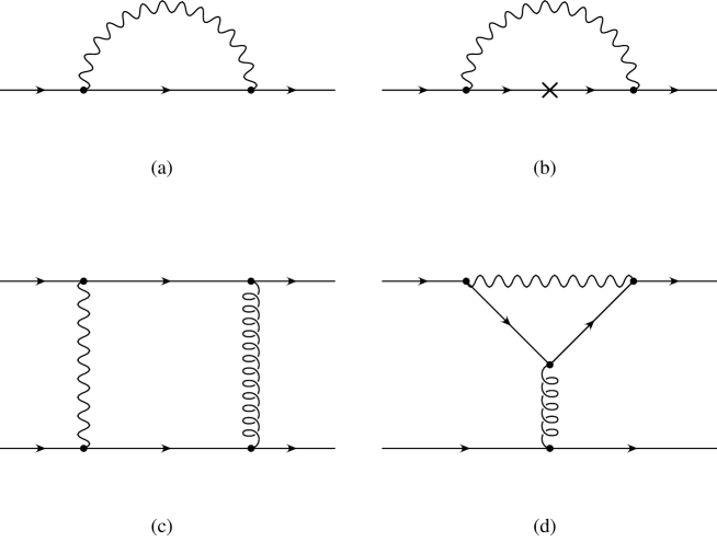
Figure 2: The short distance contributions. The wiggly line is the photon, the curly one the gluon, the full line a quark. There are also the crossed and symmetric configurations.

The contribution of the QED self-energy diagram in Figure 2(a) to the effective QCD Lagrangian, in the presence of EM virtual interactions, is

$${}-\frac{3}{2}\,\frac{\alpha}{\pi}\,\ln(\Lambda/\mu)\,\left[\left(\overline{q}_{L}\left(Q{\cal M}Q\right)^{\dagger}q_{R}\right)+\left(\overline{q}_{R}\left(Q{\cal M}Q\right)q_{L}\right)\right]\,$$ (3.5)

where colour indices are summed inside parenthesis. Its effective realization can be calculated to all orders in an $1/N_{c}$ expansion since it can be written in terms of just bilinear QCD currents. At low energies, in terms of the lowest pseudo-Goldstone bosons and external sources and at lowest order in the chiral expansion, it only contributes to the couplings $K_{10}$ and $K_{11}$ in (2.2).

$${}K_{10}^{\rm QED}=-K_{11}^{\rm QED}=\frac{3}{64\pi^{2}}\,\ln\left(\frac{\Lambda}{\mu}\right)\,.$$ (3.6)

Notice that here enters the scale $\Lambda$ where the current quark masses are defined. The remaining part of the integration from $\Lambda$ to $\infty$ is absorbed in the definition of the current quark masses. Here we can also indicate the type of corrections existing to (3.6). First, at the quark-gluon level there are $1/\mu^{2}$ and $\alpha\alpha_{S}$ corrections to (3.5). Then when going from the quark-gluon level expression in (3.5) to the hadronic level one, there are corrections that are higher order in chiral power counting. To obtain (3.6) we used the order $p^{2}$ strong Lagrangian in (2.2). There are thus CHPT ${\cal O}(p^{4})$ corrections to this result.

The presence of explicit dependence on $\Lambda$ in the short-distance contribution to $K_{10}$ and $K_{11}$ indicates that one has to be careful when using rules of the strong sector to obtain naive estimates of order of magnitude sizes of CHPT parameters. This we will refer to later as failure of naive power counting.

This problem will appear whenever non-leptonic couplings of interactions other than the strong interaction come into play. In particular it also shows up in weak non-leptonic decays. There the effects are suppressed by extra inverse powers of the $W$-boson mass, so its numerical importance is negligible.

A similar contribution comes from diagram (b) in Fig. 2. Here it is not the scalar and pseudoscalar current that are renormalized but the vector and axial-vector ones. They have to be defined at the scale $\Lambda$ and again the QED running can lead to a contribution. The cross in Fig. 2(b) denotes an insertion of an external vector or axial-vector current. This will contribute to $K_{12}$ and, with one more insertion, to $K_{13}$ and $K_{14}$. There are in principle short-distance contributions of this type but they vanish because of the global chiral invariance in QCD perturbation theory. There will be short-distance contributions from this diagram but to higher order operators in CHPT, for instance to magnetic-like structures, etc. So we have

$$K^{\rm SD}_{12}=K^{\rm SD}_{13}=K^{\rm SD}_{14}=0\,.$$ (3.7)

There can be long-distance contributions of this type due to the spontaneous breaking of the axial symmetry.

The third and fourth type of contributions to the effective Lagrangian are of order $N_{c}^{2}\alpha_{S}$. These are the well known box- and penguin-type diagrams (see Figs. 2(c) and 2(d) and crossed versions). To order $1/\mu^{2}$ they contribute to the effective Lagrangian as follows. The box-type contribution is

$$\frac{3}{2}\frac{\alpha\,\alpha^{\rm eff}_{S}(\mu^{2})}{\mu^{2}}\,{\displaystyle\sum_{a,b,c,d}}\left[\left(\overline{q}^{a}_{L}\gamma^{\mu}Q^{ab}q^{d}_{L}\right)\left(\overline{q}^{c}_{L}\gamma_{\mu}Q^{cd}q^{b}_{L}\right)\,+\,\left(\overline{q}^{a}_{R}\gamma^{\mu}Q^{ab}q^{d}_{R}\right)\left(\overline{q}^{c}_{R}\gamma_{\mu}Q^{cd}q^{b}_{R}\right)\right.$$ (3.8)

$$+ \left.4\,\left(\overline{q}^{a}_{L}Q^{ab}q^{d}_{R}\right)\left(\overline{q}^{c}_{R}Q^{cd}q^{b}_{L}\right)\right]\,.$$

and the penguin-like contribution is

$$\frac{1}{3}\frac{\alpha\,\alpha^{\rm eff}_{S}(\mu^{2})}{\mu^{2}}\,{\displaystyle\sum_{a,b,c}}\left[\left(\overline{q}^{a}_{L}\gamma^{\mu}q^{c}_{L}\right)\left(\overline{q}^{b}_{L}\gamma_{\mu}(Q^{2})^{bc}q^{a}_{L}\right)\,+\,\left(\overline{q}^{a}_{R}\gamma^{\mu}q^{c}_{R}\right)\left(\overline{q}^{b}_{R}\gamma_{\mu}(Q^{2})^{bc}q^{a}_{R}\right)\right.$$ (3.9)

$$- \left.2\,\left(\overline{q}^{a}_{L}q^{c}_{R}\right)\left(\overline{q}^{b}_{R}(Q^{2})^{bc}q^{a}_{L}\right)-2\,\left(\overline{q}^{a}_{R}q^{c}_{L}\right)\left(\overline{q}^{b}_{L}(Q^{2})^{bc}q^{a}_{R}\right)\right]\,.$$

Latin indices are for the quark flavours and colour indices are summed inside the parenthesis. The meaning of $\alpha_{S}^{\rm eff}(\mu^{2})$ is given at the end of this section. Penguin diagrams with photon and gluon interchanged does also exist but there the photon is at low energies and is thus included in the low energy part calculated in Section 3.2.

In addition there are also diagrams obtained from inserting external $v_{\mu}$, $a_{\mu}$, $s$ and $p$ currents on the internal quark lines of the box- and penguin-like diagrams in Fig. 2. These do not contribute to the effective action at order $e^{2}p^{2}$ we consider here.

The factorizable contribution (i.e. the leading order in $1/N_{c}$ contribution) to the realization of these effective Lagrangian, (LABEL:box) and (LABEL:penguin), can be easily obtained since, in that limit, this Lagrangian is just products of QCD quark currents. The low-energy realization of QCD quark currents in terms of pseudo-Goldstone bosons and external sources can be worked out in terms of the couplings appearing in the QCD chiral Lagrangian. To order $p^{2}$ this chiral Lagrangian is in (2.2), at order $p^{4}$, it can be found in [5].

Therefore, to order $p^{4}$ in the chiral expansion and leading order in $1/N_{c}$, the contributions to the couplings in (2.9) and (2.2), from integrating out virtual photons with Euclidean momentum larger than $\mu$ in (3.1) are

$${}C = \frac{3}{8}\frac{\alpha_{S}^{\rm eff}(\mu^{2})}{\pi}\frac{F_{0}^{4}B_{0\rm eff}^{2}(\mu^{2})}{\mu^{2}}\,;$$

$$\tilde{K}_{3} = \frac{3}{32}\frac{\alpha_{S}^{\rm eff}(\mu^{2})}{\pi}\frac{F_{0}^{2}}{\mu^{2}}\,;\hskip 28.45274pt\tilde{K}_{4}=0\quad;$$

$$\tilde{K}_{5}=\frac{2}{9}\left(\tilde{K}_{3}-\tilde{K}_{6}\right)\quad \quad\tilde{K}_{6}=\frac{3}{2}\,\frac{\alpha_{S}^{\rm eff}(\mu^{2})}{\pi}\frac{L_{5}B_{0\rm eff}^{2}(\mu^{2})}{\mu^{2}}\quad;$$ ;

$$K_{9} = -\frac{1}{6}\frac{\alpha_{S}^{\rm eff}(\mu^{2})}{\pi}\,\frac{(2L_{8}+H_{2})B_{0\rm eff}^{2}(\mu^{2})}{\mu^{2}}\,;$$

$$K_{10}=K^{\rm QED}_{10}-\frac{9}{2}K_{9}\, \quad K_{11}=K^{\rm QED}_{11}+\frac{3}{4}\frac{\alpha_{S}^{\rm eff}(\mu^{2})}{\pi}\,\frac{(2L_{8}-H_{2})B_{0\rm eff}^{2}(\mu^{2})}{\mu^{2}}\,.$$ ;

All others are zero because of $1/N_{c}$ counting. Here, $F_{0}\simeq$ $(86\pm 10)$ MeV is the CHPT chiral limit value of the pion decay constant $F_{\pi}$. The constants $L_{i}$ and $H_{j}$ are couplings of the order $p^{4}$ strong chiral Lagrangian in [5]. They reabsorb the UV divergences that appear in CHPT calculations to order $p^{4}$. In particular, the values of the renormalized finite parts at a CHPT scale $\tilde{\nu}=M_{\rho}$ of the constants we need in the $\overline{MS}$ scheme used in [5] are [6]: $L_{4}=-(0.3\pm 0.5)\times 10^{-3}$, $L_{5}=(1.4\pm 0.5)\times 10^{-3}$, $L_{6}=-(0.2\pm 0.3)\times 10^{-3}$, $L_{8}=(0.9\pm 0.3)\times 10^{-3}$ and $2L_{8}-H_{2}=(2.9\pm 1.0)\times 10^{-3}$ [30]. The scale dependence of the $L_{i}$ couplings cancels out when the next order in $1/N_{c}$ compared to the one in our calculation is included. We have chosen the scale $\tilde{\nu}$ to be a typical hadronic mass scale. The scales $\tilde{\nu}$, $\nu$ and $\mu$ are unrelated. The final error assigned to the short-distance contribution takes into account this $1/N_{c}$ uncertainty.

The coupling $\tilde{K}_{4}$ does not receive perturbative contributions in QCD and QED because it modulates a $L^{\mu}R_{\mu}$ two-point function. It can however receive non-perturbative contributions at leading order in $1/N_{c}$. In the case of the ENJL model, these appear proportionally to constituent quark masses.

The expressions in Eq. (3.1) have both order $p^{6}$ and $1/\mu^{4}$ corrections. The product $\alpha^{\rm eff}_{S}(\mu^{2})\,B_{0\rm eff}^{2}(\mu^{2})$ has to be understood as

$$\alpha^{\rm eff}_{S}(\mu^{2})\,B_{0\rm eff}^{2}(\mu^{2})\equiv B_{0}^{2}(1{\rm GeV}^{2})\left(\frac{\displaystyle N_{c}\alpha_{S}(1{\rm GeV}^{2})}{\displaystyle 3}\right)^{-9/11}{\displaystyle\int_{1}^{\infty}}{\rm d}x\frac{(N_{c}\alpha_{S}(x\mu^{2})/3)^{2/11}}{x^{2}}$$ (3.11)

and

$$\alpha^{\rm eff}_{S}(\mu^{2})\equiv{\displaystyle\int_{1}^{\infty}}{\rm d}x\frac{\alpha_{S}(x\mu^{2})}{x^{2}}\,.$$ (3.12)

We use the one-loop large $N_{c}$ expression

$$\alpha_{S}(\mu^{2})=\frac{12\pi}{11N_{c}\ln(\mu^{2}/\Lambda_{\rm QCD}^{2})}$$ (3.13)

with $\Lambda_{\rm QCD}=$ 300 MeV and $B_{0}(1{\rm GeV}^{2})=$1.6 GeV [30]. This corresponds to using the large $N_{c}$ renormalization group to improve the purely perturbative result.

The short-distance contributions to pseudo-Goldstone boson masses can be found in Appendix B.

We can get an estimate of the contributions suppressed in $1/N_{c}$ by keeping the leading in $1/N_{c}$ contributions from factorization in (LABEL:box) and (LABEL:penguin) at the quark-gluon level language but including the $L_{i}$ that vanish for $N_{c}\to\infty$ for the hadronic realization. This gives an additional set of nonzero terms:

$$\tilde{K}_{1}=-\frac{2}{9}\tilde{K}_{2} = -\frac{2}{3}\frac{\alpha^{\rm eff}_{S}(\mu^{2})}{\pi}\frac{L_{4}B_{0\rm eff}^{2}(\mu^{2})}{\mu^{2}}\,;$$

$$K_{7}=-\frac{2}{9}K_{8} = -\frac{4}{3}\frac{\alpha_{S}^{\rm eff}(\mu^{2})}{\pi}\frac{L_{6}B_{0\rm eff}^{2}(\mu^{2})}{\mu^{2}}\,;$$ (3.14)

3.2 Long-Distance Contribution and Matching

We need here the two-point function (3.1) for external energies up to the Euclidean scale $\mu$. This scale is expected to be around 1 GeV, thus beyond the applicability of CHPT. We therefore need to resort to models. We have chosen the ENJL model for the reasons given below in Sect. 3.2.1. The low-energy contribution to the two-point function in (3.1) was calculated already within the same ENJL model we use here in [15] for neutral pions. Here we needed to extend it to any flavour structure. Since the technique has already been explained several times[26, 31] we will not repeat it here.

Afterwards, we integrate over the photon momentum in the Euclidean space up to $r_{E}=\mu$. This gives us the lower part of the integral in (3.4).

3.2.1 The ENJL Model

For recent comprehensive reviews on the NJL [32] and the ENJL models [33], see [34, 35]. Here, we will only summarize the main features, notation and reasons why we have chosen this model. More details and some motivations on the version of the ENJL model we are using can be found in [20, 36, 37].

The kinetic part of the Lagrangian is given by

$${}{\cal L}^{\Lambda_{\rm ENJL}}_{\rm kin}=\overline{q}\left\{i\gamma^{\mu}\left(\partial_{\mu}-iv_{\mu}-ia_{\mu}\gamma_{5}-iG_{\mu}\right)-\left({\cal M}+s-ip\gamma_{5}\right)\right\}q\,.$$ (3.15)

Here summation over colour degrees of freedom is understood and we have used the following short-hand notation: $\overline{q}\equiv\left(\overline{u},\overline{d},\overline{s}\right)$; $v_{\mu}$, $a_{\mu}$, $s$ and $p$ are external vector, axial-vector, scalar and pseudoscalar field matrix sources; ${\cal M}$ is the quark-mass matrix; $G_{\mu}$ is an external colour source transforming as the gluons do in QCD. The ENJL model we are using corresponds to the following Lagrangian

$${}{\cal L}_{\rm ENJL} = {\cal L}_{\rm kin}^{\Lambda_{\rm ENJL}}+2\,g_{S}\,{\displaystyle\sum_{a,b}}\left(\overline{q}^{a}_{R}q^{b}_{L}\right)\left(\overline{q}^{b}_{L}q^{a}_{R}\right)$$ (3.16)

$$-g_{V}\,{\displaystyle\sum_{a,b}}\left[\left(\overline{q}^{a}_{L}\gamma^{\mu}q^{b}_{L}\right)\left(\overline{q}^{b}_{L}\gamma_{\mu}q^{a}_{L}\right)+\left(\overline{q}^{a}_{R}\gamma^{\mu}q^{b}_{R}\right)\left(\overline{q}^{b}_{R}\gamma_{\mu}q^{a}_{R}\right)\right]\,.$$

Here $a,b$ are flavour indices, $\Psi_{R(L)}\equiv(1/2)\left(1+(-)\gamma_{5}\right)\Psi$ and

$$g_{V}\equiv{8\pi^{2}G_{V}(\Lambda_{\rm ENJL})\over N_{c}\Lambda_{\rm ENJL}^{2}}\qquad\mbox{,}\qquad g_{S}\equiv{4\pi^{2}G_{S}(\Lambda_{\rm ENJL})\over N_{c}\Lambda_{\rm ENJL}^{2}}\,.$$ (3.17)

The couplings $G_{S}(\Lambda_{\rm ENJL})$ and $G_{V}(\Lambda_{\rm ENJL})$ are dimensionless and ${\cal O}(1)$ in the $1/N_{c}$ expansion and summation over colours between brackets in (3.16) is understood.

This model has three parameters plus the current light quark masses. The first three parameters are $G_{S}$, $G_{V}$ and the physical cut-off $\Lambda_{\rm ENJL}$ of the regularization that we chose to be proper-time. Although this regulator breaks in general the Ward identities we impose them by adding the necessary counterterms. The light quark masses in ${\cal M}$ are fixed in order to obtain the physical pion and kaon masses in the poles of the pseudoscalar two-point functions [37]. The values of the other parameters are fixed from the results of the fit to low energy effective chiral Lagrangians obtained in [36]. They are $G_{S}\simeq 1.216$, $G_{V}\simeq 1.263$, and $\Lambda_{\rm ENJL}=1.16$ GeV from Fit 1 in that reference. Solving the gap equation, we then obtain the constituent quark masses: $M_{u}=M_{d}=275$ MeV and $M_{s}=427$ MeV.

The model in (3.16) is very economical capturing in a simple fashion a lot of the observed low and intermediate energy phenomenology. It has also a few theoretical advantages.

1. The model in (3.16) has the same symmetry structure as the QCD action at leading order in $1/N_{c}$ [38]. In the chiral limit and for $G_{S}>1$ this model breaks chiral symmetry spontaneously via the expectation value of the scalar quark-antiquark one-point function (quark condensate).

2. It has very few free parameters. These are unambiguously determined from low energy physics involving only pseudo-Goldstone bosons degrees of freedom[36].

3. It only contains constituent quarks. Therefore, all the contributions to a given process are uniquely distinguished using only constituent quark diagrams. Within this model there is thus no possible double counting. In particular, the constituent quark-loop contribution and what would be the equivalent of the meson loop contributions in this model, are of different order in the $1/N_{c}$ counting. As described in [36] this model includes the constituent-quark loop model as a specific limit.

4. Resummation of fermion-loops automatically produces a pole in all main spin-isospin channels within the purely constituent quark picture. This is qualitatively the same as in the observed hadronic spectrum.

5. It provides a reasonable description of vector and axial vector meson phenomenology [39].

6. Some of the short distance behaviour is even the same as in QCD. For instance, the Weinberg sum rules [40] are satisfied. These are required in some cases for convergency, for instance in the Das et al. sum rule [2].

7. The major drawback of the ENJL model is the lack of a confinement mechanism. Although one can always introduce an ad-hoc confining potential doing the job. We smear the consequences of this drawback by working with internal and external momenta always Euclidean.

3.2.2 Extraction of the Long-Distance Contributions

The integral over the Euclidean photon momentum is done at fixed $r_{E}^{2}$, i.e. we perform the angular integration first by a Gaussian procedure. We then fit the result obtained for the two-point function (3.1) for a fixed value of the external momentum $q^{2}$ to a series of Chebyshev polynomials in $r_{E}$. The remaining integral over $r_{E}^{2}$ is then straightforward. We have choosen the $q^{2}$ points in the Euclidean region and near $q^{2}=0$ where we expect the artifacts of the model (constituent quark on-shell effects) to be suppressed.

The lower part of the integral in (3.4) has a non-analytical component too, we have however checked that, in the region of interest for $|q^{2}|\leq$ 0.2 GeV² and $r_{E}\leq$ 1 GeV the Chebyshev polynomials give a good fit and the non-analytical behaviour is actually very smooth. We have checked this by calculating the lower part of the integral within lowest order CHPT with an explicit Euclidean cut-off $\mu$. For low $\mu$ this agreed with the ENJL calculation.

The two pseudoscalar legs of the resulting two-point function are then reduced off-shell, for details of the reduction technique see [37]. Since we are working in the large $N_{c}$ limit, this has been done for the flavour structures $\overline{u}u$, $\overline{d}d$, $\overline{s}s$, $\overline{u}d$, $\overline{u}s$ and $\overline{s}d$. The CHPT expressions for these flavour combinations in the large $N_{c}$ limit after the reduction are given in Appendix A.

As an example of the quality we have shown in Fig. 3, the reduced two-point function in the chiral limit as a function of $q^{2}$ for the integral in (3.4) up to $r_{E}=$ 0.5 GeV for the charged case.

Figure 3: The long distance contribution to the reduced two-point function as a function of $q^{2}$ for the integral in (3.4) up to $\mu=r_{E}=$ 0.5 GeV. The curve is the CHPT fit. All curvature is due to the chiral log.

The curvature is purely due to the chiral logarithm. Notice that this is well reproduced by the ENJL calculation. Similar good fits were obtained for all the other combinations. From the analytic part of the fit we can then, for each flavour case, extract the combination of coupling constants as given in Appendix A.

3.2.3 Matching

Summing the short-distance calculated in the Section 3.1 and the long-distance obtained in the ENJL model we get the two-point functions in (2.1) with the two pseudoscalar sources reduced.

We have studied the matching of the long- and short-distance contributions by looking at the stability in the $\mu$ scale of the the results. We have plotted the charged pion mass difference in Figure 4.

Figure 4: The long-distance (LD), short-distance (SD) and the sum of the $N_{c}\to\infty$ results as a function of the matching scale $\mu$ for $m_{\pi^{+}}^{2}|_{\rm EM}$.

The matching is quite good above energies around (0.6 $\sim$ 0.8) GeV due to the presence of the photon propagator. This is because the presence of the photon $1/r^{2}$ propagator is enough to cut the high energy contributions. This happens despite the fact that the vector and axial-vector propagators obtained within the ENJL have only an acceptable behaviour up to around (0.5 $\sim$ 0.6) GeV in the kaon channel. We have checked that this stability (matching) region can be enlarged just by imposing the correct high-energy behaviour in the vector two-point functions coupling to the photon in this case. The predictions for the couplings remain however mostly unchanged and within the quoted errors. This is because the presence of the photon propagator suppresses these contributions.

4 Results

In this section we give the results of our calculation. In the large $N_{c}$ limit and $m_{u}=m_{d}$ there are four independent combinations of pseudoscalar two-point functions. We have calculated the following combinations at off-shell values of $q^{2}$ for our analysis:

1. Neutral case : zero quark masses, equal quark masses corresponding to the kaon mass and different quark masses corresponding to the kaon mass.

2. Charged case : zero quark masses, equal quark masses corresponding to the pion mass, equal quark masses corresponding to the kaon mass and different quark masses corresponding to the kaon mass.

To order $e^{2}p^{2}$ there appear five combinations of coupling constants. In the long distance case we have worked in the ENJL model to all orders in the chiral expansion. We will thus also obtain an estimate of the $e^{2}p^{4}$ and higher corrections to the long-distance contributions. From this analysis we have got four of the counterterms of the $e^{2}p^{2}$ Lagrangian in [12]. Remember there are ten in the large $N_{c}$ limit, where three of them involve external vector or axial-vector sources. This is presented in Section 4.2. We first extract the relevant corrections to the masses directly.

4.1 EM corrections to the Masses and Dashen’s Theorem

We take the formulas of Appendix A and fit them to the reduced two-point function of the relevant particle at a fixed value of $\mu$. We then use the same chiral formulas to extrapolate it to the pole. That way we obtain the long distance contribution to the various masses. For the short distance we take the results of Section 3.1 with $L_{4}=L_{6}=0$ to stay in the $N_{c}\to\infty$ limit. The results we obtain are given in Table 1 where we also quote the stability region. The contributions for the neutral pion are are always very small.

Particle	$m^{2}_{\rm EM}$	LD	SD	Stability
	$10^{-3}$ GeV2	$10^{-3}$ GeV2	$10^{-3}$ GeV2	$\mu$ in GeV
$\pi^{+}$	0.95	0.67	0.28	0.60 – 0.85
$K^{+}$	1.93	1.47	0.46	0.65 – 0.90
$K^{0}$	$-$0.01	$-$0.006	$-$0.004	0.65 – 0.80
$\Delta M^{2}_{EM}$	0.98	0.79	0.19	0.65 – 1.00

Table 1: The $N_{c}\to\infty$ results for the electromagnetic contributions to the meson masses squared and the violation of Dashen’s theorem. Also quoted are the long- and short-distance contribution and the stability region.

The contributions of short and long distance are both of course $\mu$-dependent. The numbers given are for the middle of the stability region. We have also quoted the result directly for the violation of Dashen’s theorem given by

$$\Delta M_{EM}^{2}\equiv\left(m_{K^{+}}^{2}-m_{K^{0}}^{2}-m_{\pi^{+}}^{2}+m_{\pi^{0}}^{2}\right)_{\rm EM}\,.$$ (4.1)

As an example of the stability we have plotted the long-distance, the short-distance and the sum of the contributions to $\left.m_{\pi^{+}}^{2}\right|_{\rm EM}$ in Fig. 4 and similar for $\Delta M_{EM}^{2}$ in Fig. 5. The matching for the other quantities is not quite as good but quite acceptable.

Figure 5: The long-distance (LD), short-distance (SD) and the sum of the $N_{c}\to\infty$ results as a function of the matching scale $\mu$ for $\Delta M_{\rm EM}^{2}$.

There are several reasons for the very good matching of $\Delta M_{EM}^{2}$. First is that in this combination, the leading effect the QED quark mass renormalization only appears multiplied by pion masses. In addition, though terms like $m_{K}^{2}\,K_{8}$ appear for individual pseudo-Goldstone boson EM corrections (in the charged pion mass for instance), they drop out in the combination $\Delta M_{\rm EM}^{2}$. Notice that these terms are $1/N_{c}$ suppressed but appear multiplied by large relative $m_{K}^{2}/m_{\pi}^{2}$ factors. The combination $\Delta M_{\rm EM}^{2}$ has no contributions from counterterms of order $e^{2}$ $p^{2}$ $1/N_{c}$. This eliminates a potentially large $1/N_{c}$ uncertainty. Therefore, EM corrections to pion and kaon masses have larger uncertainties than the combination $\Delta M_{\rm EM}^{2}$.

The above numbers are for the current quark masses defined at the scale $\Lambda=$ 1 GeV. There are contributions from QED running of pseudo-Goldstone boson masses both in the short- and long-distance counterparts. The short-distance ones are discussed in Section 3.1 and can be obtained from Eqs. (3.6). They are the terms proportional to $K_{10}^{\rm QED}$ and $K_{11}^{\rm QED}$. As discussed previously, there is a numerical ambiguity coming from this contribution. This is parametrized by the UV scale $\Lambda$ in the log dependence of the short-distance counterpart (3.5). The reason for the uncertainty is that the mass definition used here corresponds to subtracting a QED counterterm corresponding to the integral from $\Lambda$ till $\infty$. This uncertainty we estimate by varying the scale $\Lambda$. Within the context of the ENJL model (see comments in Section 3.1), one expects $\Lambda$ to vary between the rho meson mass and $\Lambda_{\rm ENJL}$, i.e. between 0.8 GeV and 1.2 GeV, roughly. The stability region we find for matching between short- and long-distance contributions is in between 0.6 GeV and 0.9 GeV. We take the variation in the contribution of $K_{10}^{\rm QED}$ and $K_{11}^{\rm QED}$ by varying the scale $\Lambda$ between 0.8 GeV and 1.2 GeV as the uncertainty due to the unknown QED counterterm. We estimate therefore this uncertainty in the pseudo-Goldstone boson masses to be lower than 1.2 $\times$ $10^{-5}$ GeV² for individual pion masses and cancelling for $(m_{\pi^{+}}^{2}-m_{\pi^{0}}^{2})_{\rm EM}$. For individual kaon masses it is smaller than 7.4 $\times$ $10^{-5}$ GeV². For the combination $\Delta M_{\rm EM}^{2}$ it is smaller than 7.5 $\times$ $10^{-6}$ GeV², thus negligible. In all cases this is smaller than other uncertainties.

The prediction we get from our calculation for $\Delta M_{\rm EM}^{2}$ due EM virtual corrections and in the large $N_{c}$ limit is

$${}\Delta M_{\rm EM}^{2}=(0.98\pm 0.30)\cdot 10^{-3}~{}{\rm GeV}^{2}\,.$$ (4.2)

We can now add the leading suppressed $1/N_{c}$ logarithmic contributions. These are the log terms proportional to $C$ in [12]. We include them at a the CHPT scale $\nu=M_{\rho}$. Notice that we are neglecting the $1/N_{c}$ contributions from the counterterms. but they cancel, as mentioned above, for the combination $\Delta M_{\rm EM}^{2}$. Using our determination of $C$ from the chiral limit two-point functions the chiral logs are the second number below

$${}\left.m^{2}_{\pi^{+}}\right|_{\rm EM}= (0.95+0.27)\cdot 10^{-3}~{}{\rm GeV}^{2} =(1.22\pm 0.40)\cdot 10^{-3}~{}{\rm GeV}^{2}$$

$$\left.m^{2}_{\pi^{0}}\right|_{\rm EM}= (0.00-0.04)\cdot 10^{-3}~{}{\rm GeV}^{2} =-(0.04\pm 0.01)\cdot 10^{-3}~{}{\rm GeV}^{2}$$

$$\left.m^{2}_{K^{+}}\right|_{\rm EM}= (1.93+0.39)\cdot 10^{-3}~{}{\rm GeV}^{2} =(2.32\pm 0.70)\cdot 10^{-3}~{}{\rm GeV}^{2}$$

$$\left.m^{2}_{K^{0}}\right|_{\rm EM}= (-0.01+0.00)\cdot 10^{-3}~{}{\rm GeV}^{2} =-(0.010\pm 0.003)\cdot 10^{-3}~{}{\rm GeV}^{2}$$

$$\Delta M^{2}_{EM}= (0.98+0.08)\cdot 10^{-3}~{}{\rm GeV}^{2} =(1.06\pm 0.32)\cdot 10^{-3}~{}{\rm GeV}^{2}$$ (4.3)

The combination $\Delta M^{2}_{\em EM}$ is calculated directly, without using the other results. This is why the error is of the same order as for the individual contributions. This is the main result of this work. We confirm a large violation of Dashen’s theorem. Some phenomenological consequences of it are discussed in Section 6.

In particular the pion mass difference result should be compared with the experimental mass difference $m^{2}_{\pi^{+}}-m^{2}_{\pi^{0}}=$ 1.26 $\cdot 10^{-3}$ GeV². As expected the experimental mass difference value $m_{\pi^{+}}^{2}-m_{\pi^{0}}^{2}$ is mostly saturated by QED virtual contributions, with $30\%$ uncertainty though. The uncertainty here due to not included $1/N_{c}$ suppressed counterterm contributions, is however larger due to the $m_{K}^{2}K_{8}$ term. An estimate of its contribution will be discussed in the next section.

4.2 Determination of Couplings of the $e^{2}p^{2}$ Lagrangian

In this section we give the value of the large $N_{c}$ couplings in (2.9) and (2.2) that can be determined from our calculation. Essentially we have fitted the CHPT large $N_{c}$ results in Eq. (A) to the output of our calculation. Being off mass-shell has allowed to determine one more coupling. See the comment about the gauge dependence of these couplings in Section 2.3. We give the central values at the points where the stability is best and the errors include typical $1/N_{c}$ error estimates as well as matching uncertainties. See the comment on matching in Section 3.2.3. As customary we take the CHPT scale $\nu$ to be the rho mass. The QED short-distance contribution in (3.6) is taken at $\Lambda=$ 1 GeV. The matching scale $\mu$ is always between 0.7 GeV and 0.9 GeV. For some combinations of couplings we do not get a very good matching contrary to the masses themselves. The variations for $\mu$ between 0.7 GeV and 0.9 GeV are still within 10% for most. This seems to be caused by the large role played by the QED mass renormalization effects. As an example we have plotted the long distance, the short distance and the sum for the coefficient $K_{10}$ in Fig. 6

Figure 6: The long-distance (LD), short-distance (SD) and the sum of the $N_{c}\to\infty$ results as a function of the matching scale $\mu$ for $K_{10}(\nu=M_{\rho})$.

and a combination with very large cancellations in Fig. 7.

Figure 7: The long-distance (LD), short-distance (SD) and the sum of the $N_{c}\to\infty$ results as a function of the matching scale $\mu$ for $\left(-2(2\tilde{K}_{3}+\tilde{K}_{4})+5(\tilde{K}_{5}+\tilde{K}_{6})-10(K_{9}+K_{10})-18K_{11}\right)(\nu=M_{\rho})$. The units are $10^{-3}$.

The other cases are somewhere in between.

From the charged combinations in the chiral limit, i.e. the zero mass charged pion case, we obtain a good matching and we obtain

$$\left.m^{2}_{\chi^{+}}\right|_{\rm EM}=\left[(0.00+0.30+0.67=0.97)\pm 0.30\right]\cdot 10^{-3}~{}{\rm GeV}^{2}$$

$${\rm at}\hskip 14.22636pt\mu=0.85~{}{\rm GeV}\,,$$ (4.4)

where the first figure is the short-distance QED contribution, the second the rest of the short-distance and the third is the long-distance part. The difference with the charged pion case is very small. Using consistently the chiral limit ENJL value $F_{0}=$ 89 MeV, we obtain for the $e^{2}p^{0}$ CHPT scale independent coefficient $C$,

$$C=\left[(0.00+1.3+2.9=4.2)\pm 1.5\right]\cdot 10^{-5}~{}{\rm GeV}^{4}\,$$

$${\rm at}\hskip 14.22636pt\mu=0.85~{}{\rm GeV}.$$ (4.5)

The central value differs by about $30\%$ from earlier determinations, e.g. [16]. There it was assumed that the full measured pion mass difference came from the $e^{2}p^{0}$ term proportional to $C$. Taking into account our error bars both results are nicely compatible, especially since the order $e^{2}p^{2}$ contribution is about 25% – see [12, 24] and the results after Eq. (4.2).

Going off-shell we can get one more combination of couplings of order $e^{2}p^{2}$, namely

$$\left(-2(2\tilde{K}_{3}+\tilde{K}_{4})+5(\tilde{K}_{5}+\tilde{K}_{6})-10(K_{9}+K_{10})-18K_{11}\right)(\nu=M_{\rho})=$$

$$\left[(0.85-2.53+2.64=0.96)\pm 0.4\right]\cdot 10^{-2}$$

$${\rm~{}at~{}}\hskip 14.22636pt\mu=0.8~{}{\rm GeV}$$ (4.6)

The three first figures are as in (LABEL:chimass).

From the neutral combinations in the chiral limit we obtain another combination of couplings, namely

$$\left(2\tilde{K}_{3}+\tilde{K}_{4}+2(\tilde{K}_{5}+\tilde{K}_{6})-4(K_{9}+K_{10})\right)(\nu=M_{\rho})=$$

$$-\left[(0.68-0.30+0.13=0.51)\pm 0.3\right]\cdot 10^{-2}$$

$${\rm~{}at~{}}\hskip 14.22636pt\mu=0.7~{}{\rm GeV}\,.$$ (4.7)

Then, by including non-zero current quark masses we can get one more coupling from the neutral combinations, namely

$$\left(K_{9}+K_{10}\right)(\nu=M_{\rho})=\left[\left(1.7+0.4+0.6=2.7\right)\pm 1.0\right]\cdot 10^{-3}$$

$${\rm~{}at~{}}\hskip 14.22636pt\mu=0.7~{}{\rm GeV}$$ (4.8)

and combining the charged combination with the chiral limit and the neutral

$$K_{10}(\nu=M_{\rho})=\left[\left(1.7+0.5+1.8=4.0\right)\pm 1.5\right]\cdot 10^{-3}$$

$${\rm~{}at~{}}\hskip 14.22636pt\mu=0.7~{}{\rm GeV}$$ (4.9)

from the charged kaon mass EM corrections. We could have used the $K_{10}$ combination from the pion mass EM corrections but the errors due to the subtraction of the chiral limit are larger. We use it as a check. Combinations of these four couplings in (LABEL:c1)-(LABEL:c4) can now be used for other predictions provided the same gauge and $\overline{MS}$ scheme we use are used too.

From the combinations of couplings above, we can obtain two combinations which are free of QED uncertainties, namely, $2\tilde{K}_{3}+\tilde{K}_{4}+2(\tilde{K}_{5}+\tilde{K}_{6})$ and $K_{9}$. In general, we see a strong dependence on the logarithmically divergent short-distance QED contribution. This makes more relevant the danger pointed out in Section 3.1 of making a naive chiral power counting here. Fortunately, as we have seen numerically in the previous section, when combined with the mass factors and electric charges, this short-distance QED contribution gives very small final contribution to the EM mass corrections.

The combinations above are determined directly from simple combinations of our results. We can combine the numbers in (LABEL:c1) to (LABEL:c4) to obtain as well

$${}K_{9}(\nu=M_{\rho}) = -1.3\cdot 10^{-3}\,,$$ (4.10)

$$K_{10}(\nu=M_{\rho}) = 4.0\cdot 10^{-3}\,,$$ (4.11)

$$\left[2\tilde{K_{3}}+\tilde{K_{4}}+2(\tilde{K_{5}}+\tilde{K_{6}})\right](\nu=M_{\rho}) = 5.7\cdot 10^{-3}\,,$$ (4.12)

$$\left[2\tilde{K_{3}}+\tilde{K_{4}}+4K_{11}\right](\nu=M_{\rho}) = -5.0\cdot 10^{-3}\,.$$ (4.13)

In view of the results we get for the couplings above, neither short-distance or long distance alone dominate any of the couplings. There are in fact large cancellations in some cases. So that not much can be said about the couplings we don’t get from our calculation.

5 Comparison with Earlier Work

Historically, the soft pion limit was used in the first attempts for estimating the EM contributions to the pions. So that, the authors in [2] arrived to the following expression for the charged pseudo-Goldstone bosons,

$${}m^{2}_{\rm EM}=\frac{e^{2}}{2F_{0}^{2}}i{\displaystyle\int}\frac{{\rm d}^{4}r}{(2\pi)^{4}}\,\frac{g_{\mu\nu}-\xi r_{\mu}r_{\nu}/r^{2}}{r^{2}-i\epsilon}\left[\Pi^{(3)\mu\nu}_{VV}(r^{2})-\Pi^{(3)\mu\nu}_{AA}(r^{2})\right]\,,$$ (5.1)

The $\Pi^{(3)}_{VV(AA)}(q^{2})$ two-point functions are

$${\Pi^{(3)\mu\nu}_{VV(AA)}}(q^{2})=$$

$$i^{2}{\displaystyle\int}{\rm d}^{4}xe^{iqx}\,\langle 0|T\left(\overline{q}(0)\gamma^{\mu}(\gamma_{5}){\displaystyle\frac{\displaystyle\lambda_{3}}{\displaystyle\sqrt{2}}}q(0)\right)\left(\overline{q}(x)\gamma^{\nu}(\gamma_{5}){\displaystyle\frac{\displaystyle\lambda_{3}^{\dagger}}{\displaystyle\sqrt{2}}}q(x)\right)|0\rangle$$

for the pions and exchanging the Gell-Mann’s flavour SU(3) matrices $\lambda_{3}^{(\dagger)}/\sqrt{2}$ by $[\lambda_{6}+(-)i\lambda_{7}]/2$ for the kaons. Neutral pseudo-Goldstone bosons get zero contribution in this limit. The sum rule in (5.1) has a good high energy behaviour in QCD due to the fulfilling of the Weinberg sum rules (WSRs) [40]. In fact, in the chiral limit, the first and second WSRs guarantee its convergency [2]. To lowest order in CHPT the integrands in (5.1) for kaons and pions are the same, this is again Dashen’s theorem.

Attempts to go beyond the approximation in (5.1) are in [12, 14, 21, 22, 24, 25]. Let us compare our results with the ones obtained in these references.

The chiral logs at $\nu=$ 1 GeV were used as an estimate of the order of magnitude of the virtual EM corrections to pseudoscalar Goldstone boson masses in [24]. This is of course a scale dependent statement, and a conclusion at any particular scale is a dangerous one. Only after adding the counterterms the result makes sense. The present work is devoted to estimate them.

In our final result (4.1), we get a relatively large violation of Dashen’s theorem, though not as large as in [25] and the same as in [21]. However, as noticed in [22], the calculation in [21] does not have the correct chiral symmetry behaviour. The short-distance contribution is here also assumed to be negligible. We find that this could be the case for scales larger than a few GeV. There is also work [42] improving the estimate made in [21]. The results found there are compatible with ours.

In Ref. [22] some VMD-like estimate in the same line as in [21] is done. The matching scale in the resonant saturation in [22] is identified wrongly with the CHPT scale, in our notation here this is setting $\mu=\nu$. This is very dangerous, since the chiral logs have in both effective theories completely different dependence. Also no attempt to make any matching of the resonant contribution with the short-distance contribution was done. These two points make it very hard for us to understand the meaning of their final result.

Splitting the different contributions to the corrections of Dashen’s lowest order result, we get

$$\frac{\left(m_{K^{+}}^{2}-m_{K^{0}}^{2}-m_{\pi^{+}}^{2}+m_{\pi^{0}}^{2}\right)_{\rm EM}}{\left(m_{\pi^{+}}^{2}-m_{\pi^{0}}^{2}\right)_{\rm exp}}=\frac{0.98+0.08}{1.26}=\,0.84\pm 0.25$$ (5.3)

where the CHPT scale of the chiral logs is taken at $\nu=M_{\rho}$. The numbers are the leading $N_{c}$ correction and the $1/N_{c}$ suppressed chiral logarithms.

Let us now compare this with what we would have gotten from a $e^{2}p^{2}$ calculation using the central values of the $K_{i}$ counterterms determined in Section 4.2 at $N_{c}\to\infty$:

$${}\Delta M_{\rm EM}^{2} = \left[\,0.94(\gamma K)-0.16(\gamma\pi)+0.53(K_{i})-0.31(L_{5}C)\,\right]\cdot 10^{-3}\,{\rm GeV}^{2}$$ (5.4)

$$= 1.00\cdot 10^{-3}\,{\rm GeV}^{2}\,.$$

The four contributions above are the photon loop contribution to the pion and the kaon, the contribution from the $K_{i}$ counterterms and the $L_{5}C$ contribution, respectively. This should be compared with $0.98\cdot 10^{-3}$ GeV² from the full calculation. The agreement is very good, remember that our nominally $e^{2}p^{2}$ couplings include also corrections to all orders in CHPT. Notice also the large cancellation between the $K_{i}$ and the $L_{5}C$ contributions, as mentioned before. The latter shows the danger of including corrections of the known constants and fully neglect the others. The statement is of course somewhat scale dependent. That the chiral logs give a sizeable part of the total result at $\nu=M_{\rho}$ is a non-trivial dynamical statement which our calculation answers.

In [12, 14] the order $e^{2}$ $p^{2}$ chiral logs together with some order of magnitude estimate of the $K_{i}$ counterterms was used. The large scale dependence of the logs only allowed to give a very broad range of results, of course compatible with the large Dashen’s violation we get.

The main difference with the calculation in [25] is the inclusion of the $1/N_{c}$ suppressed logarithms and the term proportional to $L_{5}$ (last term in (5.4)).

Recently there has been some lattice QCD results on the EM contributions to hadrons [3] using some quenched unimproved Wilson action. Their final result is $\Delta M^{2}_{\rm EM}=0.64\cdot 10^{-3}$ GeV². Unfortunately only an estimate of part of the systematic errors due to finite size effects is given there making difficult the assessment of the result. This is particularly relevant after the recent re-analyses [43] on the lattice QCD light-quark masses obtained using improved Wilson actions to calculate the same observables as in [3]. Large ${\cal O}(a)$ lattice spacing effects have been reported in those works.

There have been several other calculations in the NJL model done. These were all performed at $G_{V}=0$, keeping only the scalar four-quark operators in (3.16). One does however expect already at scales $\mu$ around 0.5 GeV (as we observe) non-negligible contributions from spin one structures. In addition they only treated the pion case, therefore we have not done a full comparison of our results with those in [44].

We can compare the determination of the couplings from the previous section with the estimates made in [12] and [13, 14]. We get that the contribution of the counterterms to $\Delta M_{\rm EM}^{2}$ is roughly one order of magnitude smaller than the estimate made in those references.

Though the coupling $K_{8}$ is $1/N_{c}$ suppressed, its contribution to the charged pion mass [12] is potentially large due to a factor $m_{K}^{2}/m_{\pi}^{2}$, as mentioned before. We can estimate the short distance estimate to $K_{8}$ from (3.1) to be around $K_{8}^{\rm SD}(\nu=M_{\rho})=-(1.0\pm 1.4)\cdot 10^{-3}$. An estimate of its total value can be done using the result in Table 1 for the pion mass difference and assuming that the deviation from the experimental result is just due to the $1/N_{c}$ counterterms proportional to $m_{K}^{2}$. Notice that we can do this because we have the complete leading in $1/N_{c}$ contributions. In that way we get $K_{8}(\nu=M_{\rho})=-(0.8\pm 2.0)\cdot 10^{-3}$, both compatible with the short-distance estimate and Zweig’s rule. In [12] this same coupling was estimated assuming that this deviation is dominated completely by the order $e^{2}p^{2}$ $K_{i}$ counterterms contributions (both leading and next-to-leading in $1/N_{c}$) proportional to $m_{K}^{2}$, so that they get $K_{8}(\nu=M_{\rho})=-(4.0\pm 1.7)\cdot 10^{-3}$.

6 Ratios of Light-Quark Masses

A combination of light current quark masses without the Kaplan-Manohar [45] ambiguity, can be obtained using the following relation [5, 46]

$${}Q^{2} \equiv \left[\left(\frac{m_{K^{+}}^{2}+m_{K^{0}}^{2}}{m_{\pi^{+}}^{2}+m_{\pi^{0}}^{2}}\right)\,\left(\frac{m_{K^{+}}^{2}+m_{K^{0}}^{2}-m_{\pi^{+}}^{2}-m_{\pi^{0}}^{2}}{2\left(m_{K^{0}}^{2}-m_{K^{+}}^{2}\right)}\right)\right]_{\rm QCD}$$ (6.1)

$$= \,\frac{4m_{s}^{2}-(m_{u}+m_{d})^{2}}{4\left(m_{d}^{2}-m_{u}^{2}\right)}\left(1\,+\,{\cal O}(m_{q}^{2}/\Lambda^{2}_{\chi})\right)\,.$$

As emphasized in [46], the higher order corrections to this particular ratio are very suppressed, so it is very constraining.

In previous sections, we have computed the virtual EM corrections to the pseudo-Goldstone bosons masses, the results are in Eq. (4.1). Subtracting them from the experimental masses we get what would be the QCD values for those masses. So the result we get for $Q$ is

$${}Q=22.0\pm 0.6$$ (6.2)

We have calculated the EM corrections at leading order in $1/N_{c}$ and to all orders in CHPT. The long distance contributions are estimated in the ENJL model and the short-distance contributions in the large $N_{c}$ limit of QCD. We also add the $1/N_{c}$ suppressed chiral logarithms to order $e^{2}p^{2}$. The uncertainty corresponds to a 30% uncertainty on our estimate of $\Delta M_{EM}^{2}$. This should be compared with the lowest order result

$$Q=24.2$$ (6.3)

using Dashen’s theorem.

The $\eta\to\pi^{+}\pi^{-}\pi^{0}$ decay rate is inversely proportional to the fourth power of $Q$ [5, 21]. Recently there has been some activity in improving the prediction of the proportionality factor [47, 48]. Comparing their best estimate with the experimental data, they get

$$Q=22.4\pm 0.9{\cite[cite]{[\@@bibref{}{KW96}{}{}]}}$$

$$Q=22.7\pm 0.8{\cite[cite]{[\@@bibref{}{AL96}{}{}]}}$$ (6.4)

in very good agreement with our result.

To obtain ratios of quark masses themselves requires extra information beyond CHPT. A very recent discussion on the consequences of values of $Q$ for the ratios of the light current quark masses can be found in [49].

7 Polarizabilities of Pseudo-Goldstone Bosons

In a previous Letter we calculated the cross-section for $\gamma\gamma\to\pi^{0}\pi^{0}$ to all orders in the chiral expansion and leading order in $1/N_{c}$ within the ENJL model[15]. As part of the work needed for this paper we need to calculate the pseudoscalar-pseudoscalar-vector-vector (PPVV) four-point function within the same model also for charged pseudoscalars and any flavour channel. We can then obtain predictions for $\gamma\gamma\to\pi^{+}\pi^{-},K^{+}K^{-},\,\bar{K}^{0}K^{0}$ to all orders in the chiral expansion and leading in the $1/N_{c}$ expansion. The cross-section for the $\gamma\gamma\to\pi^{+}\pi^{-}$ process is however dominated by the Born term and higher corrections to it are small[8, 50]. The possibility of extracting the pion polarizabilities from the $\gamma\gamma\to PP^{\dagger}$ cross-section is studied in [51]. Combining CHPT with dispersive methods they arrive to the conclusion that the predicted polarizabilities are in agreement with the experimental results. They, however, find low sensitivity in the cross-sections to the pion polarizabilities (especially to the neutral ones), so that we cannot expect a precise determination from the cross-section $\gamma\gamma\to PP^{\dagger}$. The processes $\gamma\gamma\to K^{+}K^{-},\,K^{0}\overline{K^{0}}$ occur at a too high center of mass energy for the CHPT predictions to be reliable.

The polarizabilities for the lowest pseudoscalar mesons do however fall in the regime where we expect CHPT to work. The chiral calculation for the neutral[7] and charged[8] pion polarizabilities have been performed to the two-loop level. In those works the order $p^{6}$ counterterms needed were estimated by using the resonance saturation model. Though this model has given good results to order $p^{4}$ in the strong sector [16], not much is known about its reliability at ${\cal O}(p^{6})$ (and higher). It is therefore important to compare its predictions with other models, which like the ENJL model we use, also reproduce the success of the resonance saturation predictions for the order $p^{4}$ couplings in the strong sector. Here we will provide the ENJL model estimates for them.

The polarizabilities for both $P^{+}$ and $P^{0}$ are defined by expanding the Compton amplitude in photon momenta near threshold:

$${}T\equiv 2\left[\vec{\epsilon_{1}}\cdot\vec{\epsilon_{2}}^{*}(e^{2}-4\pi\,m\,\overline{\alpha}\,\omega_{1}\,\omega_{2})-4\pi\,m\,\overline{\beta}\,(\vec{q_{1}}\times\vec{\epsilon_{1}})\cdot(\vec{q_{2}}\times\vec{\epsilon_{2}}^{*})+\cdots\right]\,;$$ (7.1)

The phase convention we use can be obtained from this amplitude definition. Here $m$ is the pseudo-Goldstone boson mass, and $q\equiv(\omega,\vec{q})$, $\vec{\epsilon}$ are the photon momentum and polarization vector, respectively. In terms of the relativistic amplitudes defined in Eq. (2) of [15] (we use the same notation as there), the polarizabilities for both neutral and charged pseudoscalar bosons are given by

$${}\overline{\alpha}-\overline{\beta} = \frac{\alpha}{m}\,{\displaystyle\lim_{s\to 0}}\,\left(\overline{A}(s,\nu=s)+8m^{2}\,\overline{B}(s,\nu=s)\right)$$

$$\overline{\alpha}+\overline{\beta} = \frac{\alpha}{m}\,{\displaystyle\lim_{s\to 0}}\,m^{2}\,\overline{B}(s,\nu=s)\,.$$ (7.2)

The barred amplitudes in (7) are the corresponding amplitudes with the Born contributions using pseudoscalar propagators to all orders in CHPT subtracted.

We have numerically calculated the full PPVV four-point function, reduced the external pseudoscalar legs (see Ref. [26]) and extracted the $A(s,\nu)$ and $B(s,\nu)$ form factors. This was done in the same way as was done in [15] for the neutral case but now we optimized the extraction for $s\approx 0$ and $t\approx m^{2}$. To order $p^{4}$ chiral symmetry imposes that $B(s,\nu)=0$. To the same order $A(s,\nu)$ also vanishes at large $N_{c}$ for the neutral pseudo-Goldstone bosons [50]. (They have however a non-zero ${\cal O}(p^{4})$ contribution from chiral logs [50].) For the charged cases ($\pi^{+}$ and $K^{+}$) we get at large $N_{c}$, i.e. only from the counterterms,

$${}A^{(4)}(s,\nu)=1.13\hskip 14.22636pt{\rm GeV}^{-2}$$ (7.3)

at leading order in the $1/N_{c}$ expansion. This compares well with the recent determination [10]

$${}A^{(4)}(s,\nu)=\frac{8}{F_{\pi}^{2}}\,\left(L_{9}+L_{10}\right)=1.5\pm 0.2\hskip 14.22636pt{\rm GeV}^{-2}.$$ (7.4)

CHPT predicts the following counterterm structure for the form factors $A(s,\nu)$ and $B(s,\nu)$

$$A(s,\nu)_{Count.} = A^{(4)}(s,\nu)+\frac{a_{1}m^{2}+a_{2}s}{\left(4\pi F_{i}\right)^{4}}\,+\,\cdots\,,$$

$$B(s,\nu)_{Count.} = \frac{b_{1}}{\left(4\pi F_{i}\right)^{4}}\,+\,\cdots$$ (7.5)

where $F_{i}$ is $F_{\pi}$ for pions and $F_{K}$ for kaons. In the ENJL model $F_{0}=89$ MeV, $F_{\pi}=90$ MeV and $F_{K}=96$ MeV at large $N_{c}$. The second term in $A(s,\nu)$ and first in $B(s,\nu)$ are the order $p^{6}$ contributions. We have fitted the $A(s,\nu)$ and $B(s,\nu)$ ENJL form factors to a polynomial in $s$ up to order $s^{2}$. These give always reasonable good fits. Thus, the $\nu^{2}$ dependence in the energy region where polarizabilities are defined is small. The results of those fits to the form factors at $A(s,\nu)$ and $B(s,\nu)$ leading order in $1/N_{c}$ in terms of $a_{1}$, $a_{2}$ and $b_{1}$ are given in Table 2 (here we consistently used the ENJL model values for $F_{0}$, $F_{\pi}$ and $F_{K}$ given above). We have done it for the chiral limit pseudo-Goldstone boson, the pion and the kaon with their appropriate masses, both for the charged and for the neutral case. The results we get from the fit for the coefficients $a_{1}$, $a_{2}$ and $b_{1}$ in Table 2 include higher than order $p^{6}$ corrections which are not of the type $s^{2}$, i.e. mainly mass corrections.

	$a_{1}$	$a_{2}$	$b_{1}$
$\chi^{+}$	–	6.7	0.38
$\pi^{+}$	$-$8.7	5.9	0.38
$K^{+}$	$-$5.6	15.8	0.77
$\chi^{0}$	–	14.0	1.66
$\pi^{0}$	$-$23.3	14.9	1.69
$K^{0}$	$-$13.2	16.9	1.10

Table 2: The dimensionless $a_{1}$, $a_{2}$ and $b_{1}$ coefficients for the chiral limit pseudo-Goldstone boson $\chi$, the pion and kaon, both for the charged and neutral ones.

The coefficients in Table 2 have a typical error estimate for the $1/N_{c}$ expansion of (20 $\sim$ 30) $\%$. In fact the difference between the coefficients $a_{2}$ and $b_{1}$ for the $\pi^{+}$ and the $K^{+}$ are higher order corrections. The coefficients $a_{1}$ of the charged pion and kaon have larger uncertainty than the rest since we get them from subtracting the dominant order $p^{4}$ contribution from the $A(s,\nu)$ form factor. From the coefficients of the chiral limit pseudo-Goldstone boson in Table 2 and the $a_{1}$ coefficients for the charged pion and kaon, one can obtain the ENJL predictions for the six terms of the order $p^{6}$ chiral Lagrangian [56] contributing to $\gamma\gamma\to PP^{\dagger}$ at large $N_{c}$.

To get the complete prediction for the polarizabilities, one has to add to the counterterm contribution we calculate within the the ENJL model to all orders in the CHPT expansion, the contributions from chiral loop diagrams (order $1/N_{c}$ in the large $N_{c}$ counting). These are for the pions known to two loops [7, 8]. Our final result for the pion and kaons polarizabilities are in Tables 3 and 4. For the SU(2) $\overline{l}_{i}$ counterterms (see [4] for their definition) entering the pion chiral log expressions we have consistently used the ENJL predicted ones, i.e.

$$\overline{l}_{1}=-1.05,\hskip 14.22636pt\overline{l}_{2}=5.8,\hskip 14.22636pt\overline{l}_{3}=2.5,\hskip 14.22636pt\overline{l}_{4}=4.3,\hskip 14.22636pt\overline{l}_{5}=14.6,\hskip 14.22636pt\overline{l}_{6}=16.9\,.$$ (7.6)

	$p^{6}$ and Higher Count.	$p^{6}$ $\chi$-logs	Total
$\pi^{0}$	0.62	0.17	0.79 $\pm$ 0.25
$\pi^{+}$	0.14	0.31	0.45 $\pm$ 0.15
$K^{0}$	1.16	–	–
$K^{+}$	0.81	–	–

Table 3: The combination of polarizabilities $\overline{\alpha}+\overline{\beta}$ in units of $10^{-4}$ fm³. The chiral logs for the kaons (Column 3) are not known.

	$p^{4}$ Count.	$p^{4}$ $\chi$-logs	$p^{6}$ and Higher Count.	$p^{6}$ $\chi$-logs	Total
$\pi^{0}$	0	$-$1.08	$-$0.47	$-$0.31	$-$1.9 $\pm$ 0.6
$\pi^{+}$	4.53	0	$-$0.25	$-$1.13	3.2 $\pm$ 1.1
$K^{0}$	0	–	$-$0.58	–	–
$K^{+}$	1.27	–	0.07	–	–

Table 4: The combination of polarizabilities $\overline{\alpha}-\overline{\beta}$ in units of $10^{-4}$ fm³. The chiral logs for the kaons (Columns 3 and 5) are not known.

The final result in Tables 3 and 4 contain the counterterm contributions to all orders in CHPT and large $N_{c}$. Notice that the experimental result from (7.4) is $(\overline{\alpha}-\overline{\beta})_{{\cal O}(p^{4})}=$ $(6.0\pm 0.8)\cdot 10^{-4}$ fm³. We can compare the counterterm entries in Tables 3 and 4 with results obtained using resonance saturation and other calculations in the ENJL model[52]. For the comparison between the resonance saturation estimates of [7] for the neutral pion case see Table 1 and text in [15]. In [8] the following results where obtained from resonance saturation for the coefficients in Table 2 in the case of the $\pi^{+}$.

$$a_{1}=-3.7\pm 1.65\,;\hskip 14.22636pta_{2}=0.75\pm 0.65\,;\hskip 14.22636ptb_{1}=0.45\pm 0.15\,.$$ (7.7)

Only $b_{1}$ seems to be in agreement, notice though that the estimates in [8] don’t include the contributions from scalar and tensor resonances. The main part of that work is however the two-loop calculation of the charged pion polarizabilities.

We disagree, as discussed in [15], with the way the order $p^{6}$ coefficients were obtained in [52]. We have not compared with the calculations in [53, 54] because they work in the ENJL model with $G_{V}=0$, so the important (even dominant) effects coming from vector and axial-vector mesons exchanges are not included. For comparison with predictions of other models for the pion polarizabilities see [55].

For a recent review of the experimental situation and data on pion polarizabilities see [7, 55] and references therein.

8 Summary and Conclusions

The main aim of this work has been the calculation of the virtual EM corrections to the masses of the pseudo-Goldstone bosons. This was motivated by some recent calculations [21, 24, 25] where large corrections to Dashen’s theorem were obtained. This was also supported by recent improved calculations of the decay rate for $\eta\to\pi^{+}\pi^{-}\pi^{0}$ [47, 48] which included estimates of higher order corrections using dispersive techniques. At the same time there appeared some works claiming that small violations of Dashen’s theorem were not excluded [12, 14, 22]. We have calculated in the large $N_{c}$ limit and using a technique similar to the one in [17] but for Green functions off-shell, the virtual EM mass corrections to pions and kaons, setting $m_{u}=m_{d}$. Our result is

$$\Delta M^{2}_{\rm EM} = \left(m_{K^{+}}^{2}-m_{K^{0}}^{2}-m_{\pi^{+}}^{2}+m_{\pi^{0}}^{2}\right)_{\rm EM}$$ (8.1)

$$= (1.06\pm 0.32)\cdot 10^{-3}~{}{\rm GeV}^{2}$$

where we have included the known $1/N_{c}$ suppressed chiral logs at order $e^{2}p^{2}$ (they are only 0.08 of that number). The error includes an estimate of the $1/N_{c}$ corrections we are missing among other uncertainties discussed along the text. Notice that the $1/N_{c}$ contribution coming from the order $e^{2}p^{2}$ counterterms cancel in the combination $\Delta M^{2}_{\rm EM}$.

Our general conclusion is that a large violation of Dashen’s theorem is quite well established. At the CHPT scale $\nu=M_{\rho}$ this is dominated by the photon loop contribution (both logs and constant pieces). In fact, our calculation is to all orders in CHPT (in the long-distance part) at large $N_{c}$, so it includes that contribution to all orders. The dominance of the photon loop contribution at $\nu=M_{\rho}$ is due to a large accidental cancellation between counterterms of order $e^{2}p^{2}$ of both types: proportional to $L_{i}C$ and $K_{i}$. The inclusion of just part of them is very dangerous at any scale. Variation of the CHPT scale in the logs should be accompanied with the running of the counterterms which could become eventually important.

A small remark here. We find some 80 $\%$ correction to the EM contribution to kaon masses (mainly from the next-to-leading order). This is very similar and consistent with what we found in another kaon self-energy quantity, the so called $B_{K}$-parameter [26]. We observe then that two-point function kaon self-energies from gauge-bosons exchange have very large higher order CHPT corrections. Notice that in our approach we are able to make a calculation to all orders in CHPT at large $N_{c}$.

We have obtained also the ratio of light quark masses $Q^{2}$ defined in (6.1),

$$Q=22.0\pm 0.6\,,$$ (8.2)

in good agreement with the one found in [47, 48]. Our result supports the very recent scheme of ratios of light-quark masses presented by Leutwyler in [49]. We have also estimated some couplings of the order $e^{2}p^{2}$ effective Lagrangian described by Urech [12]. These were all of the expected order of magnitude. For values of the combinations obtained here, see Eqs. (LABEL:c1) to (4.10).

We have discussed the ambiguity of the electromagnetic gauge choice in the definition of these couplings and pointed out how in our approach this is circumvented. We also discussed how to include the short distance renormalization needed due to photon loops.

Given the large cancellation observed here between the $K_{i}$ and the $L_{i}\,C$ counterterm contributions to electromagnetic mass differences, one should also be careful with estimates of the electromagnetic corrections to other quantities when only one of these is taken into account.

As a by-product we have also predicted the order $p^{6}$ terms which enter in the description of $\gamma\gamma\to PP^{\dagger}$ ($P=\pi^{+},\pi^{0},K^{0},K^{+}$) decays and the counterterms of electric and magnetic polarizabilities to all orders in CHPT for pions and kaons. These predictions were given in Section 7.

Appendix A EM Corrections to Pseudoscalar Two-Point Functions to ${\cal O}(e^{2}p^{2})$

In this appendix we give the large $N_{c}$ expressions for the electromagnetic contribution to the pseudoscalar two-point functions in (2.1) after reducing to order $e^{2}$ $p^{2}$ in CHPT. These are finite quantities, the coupling constants $K_{i}$ and $\tilde{K}_{i}$ are the renormalized finite parts in the $\overline{MS}$ scheme of [5] at some scale $\nu$ (this scale has nothing to do with the scale $\mu$ introduced in (3.4) or $\tilde{\nu}$ in Section 3.1).

We only give here the large $N_{c}$ expressions off mass-shell, the complete on-shell expressions to order $e^{2}$ $p^{2}$ can be found in [12] (with the translation of couplings in (2.2)). These expressions are the needed ones to obtain the large $N_{c}$ predictions for the $\tilde{K}_{i}$ and $K_{i}$ counterterms in (2.2) from our calculation. We also will use the $\overline{q}q$ basis with $q=u,d,s$ quarks which is more directly related to our large $N_{c}$ calculation. We use the Feynman gauge for the photon propagator. The reduced pseudoscalar two-point functions give the following EM corrections to the pseudo-Goldstone boson masses

$${}m^{2}_{\overline{u}u}(q^{2}) = -\frac{16e^{2}}{9}\left[q^{2}\left((2\tilde{K}_{3}+\tilde{K}_{4})\right.\right.$$

$$+ \left.\left.2(\tilde{K}_{5}+\tilde{K}_{6})-4(K_{9}+K_{10})\right)+2m_{\pi}^{2}(K_{9}+K_{10})\right]\,;$$

$$m^{2}_{\overline{d}d}(q^{2}) = \frac{1}{4}\,m^{2}_{\overline{u}u}(q^{2})\,;$$

$$m^{2}_{\overline{s}s}(q^{2}) = -\frac{4e^{2}}{9}\left[q^{2}\left((2\tilde{K}_{3}+\tilde{K}_{4})\right.\right.$$

$$+ \left.\left.2(\tilde{K}_{5}+\tilde{K}_{6})-4(K_{9}+K_{10})\right)+2(2m_{K}^{2}-m_{\pi}^{2})(K_{9}+K_{10})\right]\,;$$

$$m^{2}_{\pi^{+}}(q^{2}) = \frac{\displaystyle 2e^{2}C}{\displaystyle F_{0}^{2}}\,\left[1-8\frac{\displaystyle m_{\pi}^{2}}{\displaystyle F_{0}^{2}}L_{5}\right]-\frac{\displaystyle e^{2}}{\displaystyle 16\pi^{2}}\left[m_{\pi}^{2}\left(3\ln\left(\frac{\displaystyle m_{\pi}^{2}}{\displaystyle\nu^{2}}\right)-4\right)\right.$$

$$+ \left.2(q^{2}-m_{\pi}^{2})\left(\left(1+\frac{\displaystyle m_{\pi}^{2}}{\displaystyle q^{2}}\right)\ln\left(\frac{\displaystyle m_{\pi}^{2}-q^{2}}{\displaystyle\nu^{2}}\right)-1-\frac{\displaystyle m_{\pi}^{2}}{\displaystyle q^{2}}\ln\left(\frac{\displaystyle m_{\pi}^{2}}{\displaystyle\nu^{2}}\right)\right)\right]$$

$$- \frac{4e^{2}}{9}\left[q^{2}\left(-2(2\tilde{K}_{3}+\tilde{K}_{4})+5(\tilde{K}_{5}+\tilde{K}_{6})-10(K_{9}+K_{10})-18K_{11}\right)\right.$$

$$+ \left.m_{\pi}^{2}\left(5K_{9}-13K_{10}\right)\right]\,;$$

$$m^{2}_{K^{+}}(q^{2}) = \frac{\displaystyle 2e^{2}C}{F_{0}^{2}}\,\left[1-8\frac{\displaystyle m_{K}^{2}}{\displaystyle F_{0}^{2}}L_{5}\right]-\frac{\displaystyle e^{2}}{\displaystyle 16\pi^{2}}\left[m_{K}^{2}\left(3\ln\left(\frac{\displaystyle m_{K}^{2}}{\displaystyle\nu^{2}}\right)-4\right)\right.$$

$$+ \left.2(q^{2}-m_{K}^{2})\left(\left(1+\frac{\displaystyle m_{K}^{2}}{\displaystyle q^{2}}\right)\ln\left(\frac{\displaystyle m_{K}^{2}-q^{2}}{\displaystyle\nu^{2}}\right)-1-\frac{\displaystyle m_{K}^{2}}{\displaystyle q^{2}}\ln\left(\frac{\displaystyle m_{K}^{2}}{\displaystyle\nu^{2}}\right)\right)\right]$$

$$- \frac{4e^{2}}{9}\left[q^{2}\left(-2(2\tilde{K}_{3}+\tilde{K}_{4})+5(\tilde{K}_{5}+\tilde{K}_{6})-10(K_{9}+K_{10})-18K_{11}\right)\right.$$

$$- \left.3m_{\pi}^{2}(K_{9}+K_{10})+2m_{K}^{2}\left(4K_{9}-5K_{10}\right)\right]\,;$$

$$m^{2}_{\pi^{0}}(q^{2}) = \frac{1}{2}\left(m^{2}_{\overline{u}u}(q^{2})+m^{2}_{\overline{d}d}(q^{2})\right)\,;$$

$$m^{2}_{K^{0}}(q^{2}) = \frac{1}{2}\left(m^{2}_{\overline{d}d}(q^{2})+m^{2}_{\overline{s}s}(q^{2})\right)\,.$$ (A.1)

Appendix B Large $N_{c}$ Short-Distance Contributions

In this appendix we give the short-distance part of the EM contributions to the pseudoscalar two-point functions in (2.1) in the large $N_{c}$ limit. These are the contributions of the higher than $\mu$ photon modes to the EM corrections to these pseudoscalar two-point functions after reducing. (We only give the independent ones in the large $N_{c}$ limit.)

$$m^{2}_{\overline{u}u}(q^{2}) = -\frac{\displaystyle\alpha\alpha_{S}^{\rm eff}(\mu^{2})}{\displaystyle\mu^{2}}\frac{\displaystyle 4}{\displaystyle 27}\left[q^{2}\left(11F_{0}^{2}+112(L_{5}-(2L_{8}+H_{2}))B_{0\rm eff}^{2}(\mu^{2})\right)\right.$$

$$+ \left.56m_{\pi}^{2}(2L_{8}+H_{2})B_{0\rm eff}^{2}(\mu^{2})\right]+\frac{\displaystyle 128\pi\alpha}{\displaystyle 9}K_{10}^{\rm QED}\left(2q^{2}-m_{\pi}^{2}\right)\,;$$

$$m^{2}_{\overline{s}s}(q^{2}) = -\frac{\displaystyle\alpha\alpha_{S}^{\rm eff}(\mu^{2})}{\displaystyle\mu^{2}}\frac{\displaystyle 1}{\displaystyle 27}\left[q^{2}\left(11F_{0}^{2}+112(L_{5}-(2L_{8}+H_{2}))B_{0\rm eff}^{2}(\mu^{2})\right)\right.$$

$$+ \left.56(2m_{K}^{2}-m_{\pi}^{2})(2L_{8}+H_{2})B_{0\rm eff}^{2}(\mu^{2})\right]$$

$$+ \frac{\displaystyle 32\pi\alpha}{\displaystyle 9}K_{10}^{\rm QED}\left(2q^{2}-2m_{K}^{2}+m_{\pi}^{2}\right)\,;$$

$$m^{2}_{\pi^{+}}(q^{2}) = \frac{\alpha\alpha_{S}^{\rm eff}(\mu^{2})}{\mu^{2}}\left\{3F_{0}^{2}B_{0\rm eff}^{2}(\mu^{2})\left[1-8\frac{\displaystyle m_{\pi}^{2}}{\displaystyle F_{0}^{2}}L_{5}\right]\right.$$

$$- \frac{\displaystyle 1}{27}\left[q^{2}\left(-13F_{0}^{2}+280(L_{5}-(2L_{8}+H_{2}))B_{0\rm eff}^{2}(\mu^{2})\right.\right.$$

$$- \left.\left.\left.648(2L_{8}-H_{2})B_{0\rm eff}^{2}(\mu^{2})\right)-508m_{\pi}^{2}(2L_{8}+H_{2})B_{0\rm eff}^{2}(\mu^{2})\right]\right\}$$

$$- \frac{16\pi\alpha}{9}K_{10}^{\rm QED}\left(8q^{2}-13m_{\pi}^{2}\right)\,;$$

$$m^{2}_{K^{+}}(q^{2}) = \frac{\alpha\alpha_{S}^{\rm eff}(\mu^{2})}{\mu^{2}}\left\{3F_{0}^{2}B_{0\rm eff}^{2}(\mu^{2})\left[1-8\frac{\displaystyle m_{K}^{2}}{\displaystyle F_{0}^{2}}L_{5}\right]\right.$$ (B.1)

$$- \frac{\displaystyle 1}{27}\left[q^{2}\left(-13F_{0}^{2}+280(L_{5}-(2L_{8}+H_{2}))B_{0\rm eff}^{2}(\mu^{2})\right.\right.$$

$$- \left.648(2L_{8}-H_{2})B_{0\rm eff}^{2}(\mu^{2})\right)$$

$$- \left.\left.4(21m_{\pi}^{2}+106m_{K}^{2})(2L_{8}+H_{2})B_{0\rm eff}^{2}(\mu^{2})\right]\right\}$$

$$- \frac{16\pi\alpha}{9}K_{10}^{\rm QED}\left(8q^{2}-3m_{\pi}^{2}-10m_{K}^{2}\right)\,.$$

References

- [1]
- [2] T. Das, G.S. Guralnik, V.S. Mathur, F.E. Low, and J.E. Young, Phys. Rev. Lett. 18 (1967) 759.
- [3] A. Duncan, E. Eichten, and H. Thacker, Phys. Rev. Lett. 76 (1996) 3894; Electromagnetic Splittings and Light Quark Masses, preprint hep-lat/9609015.
- [4] J. Gasser and H. Leutwyler, Ann. of Phys., (N.Y.) 158 (1984) 142.
- [5] J. Gasser and H. Leutwyler, Nucl. Phys. B 250 (1985) 465, 517, 530.
- [6] A. Pich, Rep. Prog. Phys. 58 (1995) 563; V. Bernard, N. Kaiser, and U-.G. Meißner, Int. J. Mod. Phys. E 4 (1995) 193; G. Ecker, Prog. Part. Nucl. Phys. 35 (1995) 1.
- [7] S. Bellucci, J. Gasser, and M.E. Sainio, Nucl. Phys. B 423 (1994) 80, Erratum ibid. 431 (1994) 413.
- [8] U. Bürgi, Phys. Lett. B 377 (1996) 147; Charged Pion-Pair Production and Pion Polarizabilities to Two-Loops, Bern preprint BUTP-96/02, hep-ph/9602429, and Ph. D. Thesis, Univ. Bern (1996).
- [9] J. Bijnens, G. Colangelo, G. Ecker, J. Gasser and M. Sainio, Phys. Lett. B 374 (1996) 210.
- [10] J. Bijnens and P. Talavera, Form Factors at Two-Loops, preprint NORDITA-96/69 N,P, hep-ph/9610269 (1996), to be published in Nucl. Phys. B.
- [11] R. Dashen, Phys. Rev. 183 (1969) 1245.
- [12] R. Urech, Nucl. Phys. B 433 (1995) 234.
- [13] H. Neufeld and H. Rupertsberger, Z. Phys. C 68 (1995) 91.
- [14] H. Neufeld and H. Rupertsberger, Z. Phys. C 71 (1996) 131.
- [15] J. Bijnens, A. Fayyazuddin, and J. Prades, Phys. Lett. B 379 (1996) 209.
- [16] G. Ecker, J. Gasser, A. Pich, and E. de Rafael, Nucl. Phys. B 321 (1989) 311.
- [17] W.A. Bardeen, A.J. Buras, and J.-M. Gérard, Nucl. Phys. B 265 (1987) 787; Phys. Lett. B 192 (1987) 138.
- [18] W.A. Bardeen, J. Bijnens, and J.-M. Gérard, Phys. Rev. Lett. 62 (1989) 1343.
- [19] J.Bijnens and E. de Rafael, Phys. Lett. B 273 (1991) 483.
- [20] J. Bijnens, E. de Rafael, and H. Zheng, Z. Phys. C 62 (1994) 437.
- [21] J.F. Donoghue, B.R. Holstein, and D. Wyler, Phys. Rev. D 47 (1993) 2089.
- [22] R. Baur and R. Urech, Phys. Rev. D 53 (1996) 6552.
- [23] R.H. Socolow, Phys. Rev. 137 (1965) B1221; Riazuddin, Phys. Rev 114 (1959) 1184.
- [24] P. Langacker and H. Pagels, Phys. Rev. D 8 (1973) 4620; K. Maltman and D. Kotchan, Mod. Phys. Lett. A5 (1990) 2457; G. Stephenson, K. Maltman, and D. Kotchan, Phys. Rev. 43 (1991) 860.
- [25] J. Bijnens, Phys. Lett. B 306 (1993) 343.
- [26] J. Bijnens and J. Prades, Nucl. Phys. B 444 (1995) 523, Phys. Lett. B 342 (1995) 331.
- [27] S. Weinberg, Physica A 96 (1979) 327.
- [28] P. Di Vecchia and G. Veneziano, Nucl. Phys. B 171 (1980) 253 ; C. Rosenzweig, J. Schechter, and T. Trahern, Phys. Rev. D 21 (1980) 3388; E. Witten, Ann. Phys. (N.Y.) 128 (1980) 363.
- [29] S. Peris and E. de Rafael, Phys. Lett. B348 (1995) 539.
- [30] J. Bijnens, J. Prades, and E. de Rafael, Phys. Lett. B 348 (1995) 226.
- [31] J. Bijnens, E. Pallante, and J. Prades, Phys. Rev. Lett. 75 (1995) 1447, Erratum ibid. 75 (1995) 3781, Nucl. Phys. B474 (1996) 379.
- [32] Y. Nambu and G. Jona-Lasinio, Phys. Rev. 122 (1961) 345, ibid. 124 (1961) 246.
-
[33]
H. Kleinert, Phys. Lett. B59 (1975) 163, B62 (1976) 429;
A. Dhar, R. Shankar and S.R. Wadia, Phys. Rev. D31 (1985) 3256;
S.R. Wadia, Prog. Theor. Phys. Suppl. 86 (1986) 26 ;
D. Ebert and H. Reinhardt, Nucl. Phys. B271 (1986) 188. - [34] T. Hatsuda and T. Kunihiro, Phys. Rep. 247 (1994) 221.
- [35] J. Bijnens, Phys. Rep. 265 (1996) 369.
- [36] J. Bijnens, C. Bruno, and E. de Rafael, Nucl. Phys. B 390 (1993) 501.
- [37] J. Bijnens and J. Prades, Z. Phys. C 64 (1994) 475.
- [38] G. ’t Hooft, Nucl. Phys. B 72 (1974) 461.
- [39] J. Prades, Z. Phys. C 63 (1994) 491.
- [40] S. Weinberg, Phys. Rev. Lett. 18 (1967) 507.
- [41] S. Peris, M. Perrottet, and E. de Rafael, in preparation.
- [42] J.F. Donoghue and A.F. Pérez, The Electromagnetic Mass Differences of Pions and Kaons, Cincinnati preprint UCTP-9-96, Amherst preprint UMHEP-428, hep-ph/9611331.
- [43] R. Gupta and T. Bhattacharya, Light Quark Masses from Lattice QCD, Los Alamos preprint LAUR-96-1840, hep-lat/9605039; B.J. Gough et al. The Light Quark Masses from Lattice Gauge Theory, preprint Fermilab Pub-96-283, Illinois ILL-TH-96-07, Hiroshima HUPD-961, hep-lat/9610223. P.B. Mackenzie, Recent Lattice Results on the Light Quark Masses, hep-ph/9609261.
- [44] V. Dmitrasinovic, H.J. Schulze, R. Tegen, and R. Lemmer, Phys. Rev. D 52 (1995) 2855.
- [45] D.B. Kaplan and A.V. Manohar, Phys. Rev. Lett. 56 (1986) 2004.
- [46] J. Gasser and H. Leutwyler, Phys. Rep. 87 (1982) 77.
- [47] J. Kambor, C. Wiesendanger, and D. Wyler, Nucl. Phys. B 465 (1996) 215.
- [48] A.V. Anisovich and H. Leutwyler, Phys. Lett. B 375 (1996) 335.
- [49] H. Leutwyler, Light Quark Masses, Bern preprint hep-ph/9609467 and references therein.
- [50] J. Bijnens and F. Cornet, Nucl. Phys. B 296 (1988) 557.
- [51] J.F. Donoghue and B.R. Holstein, Phys. Rev. D 48 (1993) 137.
- [52] S. Bellucci and C. Bruno, Nucl. Phys. B 452 (1995) 626.
- [53] V. Bernard and D. Vautherin, Phys. Rev. D 40 (1989) 1615.
- [54] B. Bajc, A.H. Blin, M.C. Nemes, A.A. Osipov, and M. Rosina, Nucl. Phys. A 604 (1996) 406.
- [55] M.R. Pennington and J. Portolés, “The Second DANE Physics Handbook”, L. Maiani, G. Pancheri, and N. Paver (eds.) 1995, p. 579.
- [56] H. Fearing and S. Scherer, Phys. Rev. D53 (1996) 315.