An Analysis of $\pi\pi$-Scattering Phase Shift
and Existence of ${\bf\sigma(555)}$ particle

1 Introduction

Chiral symmetry has a long history in particle physics and has played a central role in understanding the spectroscopy of hadrons with light flavors: In particular it is now widely accepted that the $\pi$-meson (or pseudo-scalar meson nonet) has the properties of a Nambu-Goldstone boson, corresponding to the dynamical breaking of chiral symmetry (D$\chi$SB) in the massless limit of QCD.

In the Nambu$\cdot$Jona-Lasinio (NJL) model[1] and its extended version (ENJL)[2] adapted to the quark model, which simply realizes the physical situation of D$\chi$SB, the existence of the $\sigma$-meson (or scalar meson nonet) is predicted as a chiral partner of $\pi$ (or a pseudo-scalar meson nonet), with iso-spin I=0 and mass=$2m_{q}$ ($m_{q}$ being the constituent quark mass).

It is also well-known that, in the investigation of nuclear forces with one-boson-exchange potential,[3] an iso-singlet scalar particle with mass of about 500MeV, which can possibly be identified with the $\sigma$ (or a strongly correlated two-pion state [4]), is necessary. However, the existence of $\sigma$ as a resonant particle has not yet been generally accepted. A major reason for this is due to the analyses of $\pi\pi$ phase-shift obtained from the high-statistics data of a CERN-Münich experiment[5] in 1974, in which the phase shift $\delta_{0}^{0}$ up to $m_{\pi\pi}=1300{\rm MeV}$ turned out to be only 270^∘. Accordingly, after subtracting a rapid contribution of the resonance $f_{0}(980)$$(180^{\circ})$, there remains only $90^{\circ}$, which is insufficient for $\sigma$ around $m$=$2m_{q}$=$500\sim 600{\rm MeV}$, and many analyses thus far made on the phase shift have yielded conclusions against the existence of $\sigma$. [6, 7, 8]

Reflecting this situation, the non-linear realization of chiral symmetry now seems to be widely believed rather than the simple linear representation in the NJL model. In this case, the existence of $\sigma$ (or a scalar nonet in ENJL) is unnecessary, which is represented as a function of $\pi$ (or a pseudo-scalar meson nonet).

On the other hand, the possible existence of $\sigma$ has been suggested from various viewpoints [14] both theoretically and phenomenologically. [15, 16, 17, 18] In particular the importance of $\sigma$ in relation with the D$\chi$SB has been argued extensively by Refs.?, ?, ?.

Here, it may be worthwhile to note that in a recent $pp$ central collision experiment, an event concentration in the I=0, $S$-wave $\pi\pi$ channel is seen [22] in the region of $m_{\pi\pi}$ around $500\sim 600{\rm MeV}$, which is too large to be explained as a simple “background” and seems strongly to suggest the existence of $\sigma$ (a brief review is given in §4(B)).

Considering all the above situations, a more rigorous re-analysis of $\pi\pi$-phase shift seems to be necessary.

In this paper, the authors will perform this by applying a new method of analysis, the Interfering-Amplitude (IA) method, which is able to treat partial-wave multi-resonances directly in the ${\cal T}$-matrix (instead of in the most conventionally used ${\cal K}$-matrix) in conformity with unitarity in the final state $\pi\pi$-interactions. As a result, evidence for the existence of the $\sigma$-meson is shown from the characteristic behavior of the $\pi\pi\rightarrow\pi\pi$ phase shift under the $K\overline{K}$ threshold. A keystone for this is the introduction of a negative background phase, due to an unknown repulsive force between pions, which might suggest the existence of a repulsive core in the $\pi\pi$ interaction. Here it is notable that the existence of a similar negative background phase has been established phenomenologically in the case of the $N$-$N$-interaction.

In §2, the IA Method is introduced. Its relation to other approaches, such as the ${\cal K}$-matrix method, is discussed in §4(A).

In §3, the $\pi\pi$ scattering phase shift is re-analyzed by applying the IA method. It is especially shown that the characteristic features of phase shifts from the $\pi\pi$- to the $K\overline{K}$- thresholds, including a small bump around 750MeV, are reproduced well with our new background phase and the $\sigma$ with mass of 555MeV.

The properties of $f_{0}(980)$ are also examined with the data including those over the $K\overline{K}$ threshold in this section. Its width attains a value from tens MeV[7] to hundreds of MeV,[10] largely depending upon the treatment of the elasticity and the $\pi\pi\rightarrow K\overline{K}$ phase shift, both of which have large experimental uncertainties.

In §4(C) we give some arguments on the repulsive core in the $\pi\pi$-interactions, a possible physical origin of the negative-phase background. It is pointed out that our best fit value of the core radius is almost equal to the structural size of the pion, showing a similarity to the case of the $N$-$N$ interaction, where the core radius has an order of the size of a nucleon.

In §4(D) the existence of new types of $0^{++}$ and $1^{++}$ nonets is suggested. These are outside of the normal L-excited meson nonets. $\sigma$ seems to have properties such that it should be assigned as a member of this new type of scalar nonet.

2 Partial-wave multi-resonance and interfering-amplitude method

In extracting resonances due to physical particles from scattering amplitudes, we usually fit partial wave amplitudes with the Breit-Wigner(BW) form. The scattering matrix $S$ must satisfy unitarity, which means conservation of probability from initial to final states:

$$SS^{{\dagger}}=S^{{\dagger}}S=1.$$ (2.1)

We shall treat the $\pi\pi$ $S$-wave scattering in case of two relevant channels: $\pi\pi$ and $K\overline{K}$, denoted as channels 1 and 2, respectively. In this case the $\rho$ matrix has a diagonal form

$$\rho = diag(\frac{|{\bf p}_{1}|}{8\pi\sqrt{s}},\frac{|{\bf p}_{2}|}{8\pi\sqrt{s}}),$$

$$|{\bf p}_{1}| = \sqrt{\frac{s}{4}-m_{\pi}^{2}},\ |{\bf p}_{2}|=\sqrt{\frac{s}{4}-m_{K}^{2}},$$ (2.2)

The partial wave scattering matrix $S^{l}$ is defined as

$$S_{\bf ji} = (2\pi)^{4}\delta^{(4)}(P_{j}-P_{i})\sqrt{\frac{1}{\rho_{j}\rho_{i}}}\sum_{l=0}^{\infty}\frac{2l+1}{2}P_{l}({\bf n}\cdot{\bf n}^{\prime})S_{ji}^{l},$$ (2.3)

where the suffix j(i) represents the final (initial) channel, ${\bf n}^{\prime}$(${\bf n}$) is a unit vector of 3-momentum of the first particle in the final (initial) system. The bold suffices j, i include momenta of the system.

The unitarity equation (2.1) is represented, in terms of $S^{l}$, as

$$S^{l}_{jk}S^{l{\dagger}}_{ki}=\delta_{ji};\ \ \ l=0,1,2,....$$ (2.4)

The $S^{l}$ matrix is symmetric due to time reversal invariance

$$S^{l}_{ji}=S^{l}_{ij}.$$ (2.5)

The ${\cal T}$-matrix and its partial wave component ${\cal T}^{l}$ are usually defined, for relevant systems of two spinless particles as

$$\halign to=0.0pt{\@eqnsel\hskip\@centering$\displaystyle{#}$&\global\@eqcnt\@ne\hskip 2\arraycolsep\hfil${#}$\hfil&\global\@eqcnt\tw@\hskip 2\arraycolsep$\displaystyle{#}$\hfil&\llap{#}\cr 0.0pt plus 1000.0pt$\displaystyle{S_{\bf ji}&12.0pt\hfil${=&12.0pt$\displaystyle{\delta_{\bf ji}-i(2\pi)^{4} \delta^{(4)}(P_{j}-P_{i}){\cal T}_{\bf ji}, {}&\hbox to0.0pt{\hss{\rm(2\raise 2.15277pt\hbox{.}6a)}\cr\penalty 100\vskip 3.0pt\vskip 0.0pt\cr 0.0pt plus 1000.0pt$\displaystyle{{\cal T}_{\bf ji}&12.0pt\hfil${=&12.0pt$\displaystyle{\sum_{l}(2l+1)P_{l} ({\bf n} \cdot{\bf n}') {\cal T}_{ji}^{l}. &\hbox to0.0pt{\hss{\rm(2\raise 2.15277pt\hbox{.}6b)}\cr}}}}}}}}}$$

The $S^{l}$ is related to ${\cal T}^{l}$ as

$$S_{ji}^{l} = \delta_{ji}-2i\sqrt{\rho_{j}\rho_{i}}{\cal T}_{ji}^{l}.$$ (2.7)

Equations (2.4) and (2.5) are equivalent, respectively, to the following conditions on ${\cal T}_{ji}^{l}$:

$$i({\cal T}_{ji}^{l} - {\cal T}_{ji}^{l{\dagger}})=2({\cal T}^{l}\rho{\cal T}^{l{\dagger}})_{ji},$$ (2.8)

$${\cal T}^{l}_{ji} = {\cal T}^{l}_{ij}.$$ (2.9)

In the case with only one resonance, these conditions are satisfied by the BW amplitude. However, in the case of “multi-resonance scattering” (when many resonances exist with the same quantum number), if we represent the partial wave ${\cal T}$ matrix as a simple sum of corresponding BW formulae, they are not satisfied.

Here we give a new method for describing the scattering amplitude in conformity with the unitarity relation in this case.

We shall treat directly the partial wave amplitude defined as

$$a_{ji}^{l} \equiv -\sqrt{\rho_{j}\rho_{i}}{\cal T}_{ji}^{l},$$ (2.10)

which is related to $S^{l}$ as

$$S_{ji}^{l} = \delta_{ji}+2ia_{ji}^{l}.$$ (2.11)

In the following we treat only $a^{l}_{ji}$ (or $S^{l}_{ji}$) with $l=0$, and the superscript $l$ is omitted.

2.1. one-channel multi-resonance scattering amplitude

First let us consider the one channel case.

A basic idea of our method is that a phase shift $\delta(s)$ of the scattering amplitude is essentially only due to physical particle resonances through the BW formulae, and the phases of multi-resonances contribute additively to $\delta(s)$. Thus it is represented as

$$\delta(s)=\delta^{Re}=\stackrel{{\scriptstyle(1)}}{{\delta}}+\stackrel{{\scriptstyle(2)}}{{\delta}}+\stackrel{{\scriptstyle(3)}}{{\delta}}+\cdots\ ,$$ (2.12)

where $\stackrel{{\scriptstyle(i)}}{{\delta}}$ is a real phase coming from the i-th resonance.

In the case with one-resonance, the scattering matrix is given as

$$\stackrel{{\scriptstyle(1)}}{{S}}=e^{2i\stackrel{{\scriptstyle(1)}}{{\delta}}}=1+2i\stackrel{{\scriptstyle(1)}}{{a}},$$ (2.13)

by the BW formula

$$\stackrel{{\scriptstyle(1)}}{{a}} = \frac{-\sqrt{s}\mathchar 28928\relax_{(1)}^{1}(s)}{s-M_{(1)}^{2}+i\sqrt{s}\mathchar 28928\relax_{(1)}^{1}(s)},\ \ \ \sqrt{s}\mathchar 28928\relax_{(1)}^{1}(s)=\frac{|{\bf p}_{1}|}{8\pi\sqrt{s}}\stackrel{{\scriptstyle(1)}}{{g}}^{2}_{1}=\rho_{1}(s)\stackrel{{\scriptstyle(1)}}{{g}}^{2}_{1}.$$ (2.14)

The $\stackrel{{\scriptstyle(1)}}{{\delta}}$ is real, as is seen by substituting Eq.(2.14) into Eq.(2.13), and the unitarity relation $SS^{*}=1$, Eq.(2.4), is easily shown to be satisfied.

In the two-resonance case the scattering matrix,

$$S = e^{2i\delta(s)}=1+2ia(s),$$ (2.15)

is given as a multiplicative form of the “respective resonance $S$-matrices” $\stackrel{{\scriptstyle(i)}}{{S}}=e^{2i\stackrel{{\scriptstyle(i)}}{{\delta}}}=1+2i\stackrel{{\scriptstyle(i)}}{{a}}$ as

$$S = \stackrel{{\scriptstyle(1)}}{{S}}\stackrel{{\scriptstyle(2)}}{{S}}.$$ (2.16)

The unitarity relation $SS^{*}=1$ is easily seen to be satisfied by the “unitarity of respective $\stackrel{{\scriptstyle(i)}}{{S}}$.” The scattering amplitude $a(s)$ ($=-\rho_{1}(s){\cal T}(s)$) is represented, in terms of the respective BW resonances, as

$$a(s)=\stackrel{{\scriptstyle(1)}}{{a}}(s)+\stackrel{{\scriptstyle(2)}}{{a}}(s)+2i\stackrel{{\scriptstyle(1)}}{{a}}(s)\stackrel{{\scriptstyle(2)}}{{a}}(s).$$ (2.17)

This amplitude consists of a simple sum of respective BW resonances and their cross term ($2i\stackrel{{\scriptstyle(1)}}{{a}}(s)\stackrel{{\scriptstyle(2)}}{{a}}(s)$). The latter, which looks like an “interference” of the former two resonances, appears in the amplitude. Thus we call this method of constructing the amplitudes the Interfering-Amplitude (IA) method.

Extension to the three-resonance case is straightforward, and the formulae are given as

$$S = e^{2i(\stackrel{{\scriptstyle(1)}}{{\delta}}+\stackrel{{\scriptstyle(2)}}{{\delta}}+\stackrel{{\scriptstyle(3)}}{{\delta}})}=\stackrel{{\scriptstyle(1)}}{{S}}\stackrel{{\scriptstyle(2)}}{{S}}\stackrel{{\scriptstyle(3)}}{{S}},$$ (2.18)

$$a(s) = \stackrel{{\scriptstyle(1)}}{{a}}+\stackrel{{\scriptstyle(2)}}{{a}}+\stackrel{{\scriptstyle(3)}}{{a}}+2i(\stackrel{{\scriptstyle(1)}}{{a}}\stackrel{{\scriptstyle(2)}}{{a}}+\stackrel{{\scriptstyle(2)}}{{a}}\stackrel{{\scriptstyle(3)}}{{a}}+\stackrel{{\scriptstyle(3)}}{{a}}\stackrel{{\scriptstyle(1)}}{{a}})-4\stackrel{{\scriptstyle(1)}}{{a}}\stackrel{{\scriptstyle(2)}}{{a}}\stackrel{{\scriptstyle(3)}}{{a}}.$$ (2.19)

A background phase $\delta^{BG}$ is added to the phase shift Eq.(2.12), if necessary:

$$\delta=\delta^{Re}+\delta^{BG}.$$ (2.20)

The unitarity relation is satisfied for any real $\delta^{BG}$. In this case the scattering amplitude is given by a background amplitude $a^{BG}$ and the resonance amplitude $a^{Re}$ (Eqs.(2.17) and (2.19)) as

$$a=a^{BG}+a^{Re}+2ia^{BG}a^{Re}=a^{BG}+a^{Re}e^{2i\delta^{BG}},$$ (2.21)

where

$$a^{BG}\equiv\frac{e^{2i\delta^{BG}}-1}{2i}.$$

Application to the greater than three-resonance case can be done in a similar way.

2.2. two-channel multi-resonance scattering amplitude

Next we construct an explicit form of the scattering amplitude in the two-channel case. We treat scattering matrix elements $S_{11}$, $S_{12}$ and $S_{22}$. The element $S_{21}$ is equal to $S_{12}$ by time reversal invariance (Eq.(2.5)). On these three elements is imposed the unitarity relation (Eq.(2.4))

$$|S_{11}|^{2}+|S_{12}|^{2} = |S_{22}|^{2}+|S_{12}|^{2}=1,$$

$$S_{11}S_{12}^{*} + S_{12}S_{22}^{*}=0.$$ (2.22)

The form of $S_{ij}$, satisfying the above equations, is written as

$$S_{11} \equiv \eta e^{2i\delta},$$

$$S_{12} \equiv \sqrt{1-\eta^{2}}e^{i(\phi+\frac{\pi}{2})},$$

$$S_{22} \equiv \eta e^{2i\delta^{\prime}},$$ (2.23)

in terms of the phase shift $\delta(\delta^{\prime})$ in the $\pi\pi(K\overline{K})$ scattering, the corresponding elasticity $\eta(=\eta^{\prime})$, and the phase $\phi$ in the $\pi\pi\rightarrow K\overline{K}$ scattering. These phases are constrained by

$$\delta+\delta^{\prime}=\phi.$$ (2.24)

In the one-resonance case, the scattering matrix elements satisfying the unitarity relation Eq.(2.22) are given in terms of the BW amplitude as

$$\stackrel{{\scriptstyle(1)}}{{S}}_{11} = 1+2i\stackrel{{\scriptstyle(1)}}{{a}}_{11},\ \stackrel{{\scriptstyle(1)}}{{S}}_{12}=2i\stackrel{{\scriptstyle(1)}}{{a}}_{12},\ \stackrel{{\scriptstyle(1)}}{{S}}_{22}=1+2i\stackrel{{\scriptstyle(1)}}{{a}}_{22},$$ (2.25)

$$\stackrel{{\scriptstyle(1)}}{{a}}_{ij} = \frac{-\sqrt{\sqrt{s}\mathchar 28928\relax_{(1)}^{i}\sqrt{s}\mathchar 28928\relax_{(1)}^{j}}}{s-M_{(1)}^{2}+i\sqrt{s}\mathchar 28928\relax_{(1)}^{tot}(s)},\ \ \ \mathchar 28928\relax_{(1)}^{tot}(s)=\mathchar 28928\relax_{(1)}^{1}(s)+\mathchar 28928\relax_{(1)}^{2}(s).$$ (2.26)

Phases $\delta$ and $\phi$ are obtained by comparing Eqs.(2.25) and (2.26) with their definition Eq.(2.23), and the elasticity $\eta$ is given as

$$\stackrel{{\scriptstyle(1)}}{{\eta}}=\sqrt{1-4\frac{\sqrt{s}\mathchar 28928\relax_{(1)}^{1}(s)\sqrt{s}\mathchar 28928\relax_{(1)}^{2}(s)}{(s-M_{(1)}^{2})^{2}+(\sqrt{s}\mathchar 28928\relax_{(1)}^{tot}(s))^{2}}}.$$ (2.27)

In the two-resonance case, extending the method in Eq.(2.16) to this case, the diagonal elements of the scattering matrix, $S_{11}$ and $S_{22}$, are represented in a multiplicative form of respective resonance $S$-matrices

$$\halign to=0.0pt{\@eqnsel\hskip\@centering$\displaystyle{#}$&\global\@eqcnt\@ne\hskip 2\arraycolsep\hfil${#}$\hfil&\global\@eqcnt\tw@\hskip 2\arraycolsep$\displaystyle{#}$\hfil&\llap{#}\cr 0.0pt plus 1000.0pt$\displaystyle{ S_{11} &12.0pt\hfil${=&12.0pt$\displaystyle{\stackrel{{\scriptstyle(1)}}{{S}}_{11}\stackrel{{\scriptstyle(2)}}{{S}}_{11},\ S_{22} = \stackrel{{\scriptstyle(1)}}{{S}}_{22}\stackrel{{\scriptstyle(2)}}{{S}}_{22}, {}&\hbox to0.0pt{\hss{\rm(2\raise 2.15277pt\hbox{.}28a)}\cr\penalty 100\vskip 3.0pt\vskip 0.0pt\cr 0.0pt plus 1000.0pt$\displaystyle{\stackrel{{\scriptstyle(i)}}{{S}}_{11} &12.0pt\hfil${=&12.0pt$\displaystyle{\stackrel{{\scriptstyle(i)}}{{\eta}} e^{2i\stackrel{{\scriptstyle(i)}}{{\delta}}},\ \stackrel{{\scriptstyle(i)}}{{S}}_{22} =\stackrel{{\scriptstyle(i)}}{{\eta}} e^{2i\stackrel{{\scriptstyle(i)}}{{\delta'}}}, &\hbox to0.0pt{\hss{\rm(2\raise 2.15277pt\hbox{.}28b)}\cr}}}}}}}}}$$

where the elasticity $\eta$ in each diagonal channel is represented in the multiplicative form $\eta=\stackrel{{\scriptstyle(1)}}{{\eta}}\stackrel{{\scriptstyle(2)}}{{\eta}}$, and the phase shift as a sum $\delta=\stackrel{{\scriptstyle(1)}}{{\delta}}+\stackrel{{\scriptstyle(2)}}{{\delta}}$, following from its physical meaning. Corresponding amplitudes are given in a form similar to Eq.(2.17) in the one-channel case:

$$a_{11} = \frac{S_{11}-1}{2i}=\stackrel{{\scriptstyle(1)}}{{a}}_{11}+\stackrel{{\scriptstyle(2)}}{{a}}_{11}+2i\stackrel{{\scriptstyle(1)}}{{a}}_{11}\stackrel{{\scriptstyle(2)}}{{a}}_{11},$$

$$a_{22} = \frac{S_{22}-1}{2i}=\stackrel{{\scriptstyle(1)}}{{a}}_{22}+\stackrel{{\scriptstyle(2)}}{{a}}_{22}+2i\stackrel{{\scriptstyle(1)}}{{a}}_{22}\stackrel{{\scriptstyle(2)}}{{a}}_{22}.$$ (2.29)

The non-diagonal $S$-matrix element is determined through relations (2.23) and (2.24) with the diagonal elements given above. First, the phase shift $\phi$ of $S_{12}$ is equal to a sum of respective contributions of resonances: $\phi=\stackrel{{\scriptstyle(1)}}{{\phi}}+\stackrel{{\scriptstyle(2)}}{{\phi}}$. So it becomes of the form $S_{12}=2i\stackrel{{\scriptstyle(1)}}{{a}}_{12}\times\stackrel{{\scriptstyle(2)}}{{a}}_{12}\times$(real function). The absolute value of $S_{12}$ is determined by Eq.(2.22)

$$S_{12}=-i\stackrel{{\scriptstyle(1)}}{{a}}_{12}\stackrel{{\scriptstyle(2)}}{{a}}_{12}\frac{\sqrt{1-\eta^{2}}}{|\stackrel{{\scriptstyle(1)}}{{a}}_{12}\stackrel{{\scriptstyle(2)}}{{a}}_{12}|}\equiv 2ia_{12}.$$ (2.30)

The unitarity Eq.(2.22) is guaranteed by the above procedure to derive $S_{12}$.

Extension to the three-resonance case can be done in the same manner. The results are given as

$$S_{ii} = \stackrel{{\scriptstyle(1)}}{{S}}_{ii}\stackrel{{\scriptstyle(2)}}{{S}}_{ii}\stackrel{{\scriptstyle(3)}}{{S}}_{ii}\ \ \ {\rm for}\ \ i=1,2\ ,$$

$$S_{12} = -i\stackrel{{\scriptstyle(1)}}{{a}}_{12}\stackrel{{\scriptstyle(2)}}{{a}}_{12}\stackrel{{\scriptstyle(3)}}{{a}}_{12}\frac{\sqrt{1-\eta^{2}}}{|\stackrel{{\scriptstyle(1)}}{{a}}_{12}\stackrel{{\scriptstyle(2)}}{{a}}_{12}\stackrel{{\scriptstyle(3)}}{{a}}_{12}|},$$

$$\eta = \stackrel{{\scriptstyle(1)}}{{\eta}}\stackrel{{\scriptstyle(2)}}{{\eta}}\stackrel{{\scriptstyle(3)}}{{\eta}},$$ (2.31)

$$a_{ii} = \stackrel{{\scriptstyle(1)}}{{a}}_{ii}+\stackrel{{\scriptstyle(2)}}{{a}}_{ii}+\stackrel{{\scriptstyle(3)}}{{a}}_{ii}+2i(\stackrel{{\scriptstyle(1)}}{{a}}_{ii}\stackrel{{\scriptstyle(2)}}{{a}}_{ii}+\stackrel{{\scriptstyle(2)}}{{a}}_{ii}\stackrel{{\scriptstyle(3)}}{{a}}_{ii}+\stackrel{{\scriptstyle(3)}}{{a}}_{ii}\stackrel{{\scriptstyle(1)}}{{a}}_{ii})-4\stackrel{{\scriptstyle(1)}}{{a}}_{ii}\stackrel{{\scriptstyle(2)}}{{a}}_{ii}\stackrel{{\scriptstyle(3)}}{{a}}_{ii},$$

$$a_{12} = \frac{S_{12}}{2i}.$$ (2.32)

Here, it may be worthwhile to note that all phases, $\delta(s),\delta^{\prime}(s)$ and $\phi(s)$, are given as a sum of contributions of respective resonances as in Eq.(2.12). Application to the greater than three-resonance case can be done in a similar way.

Background phases are added to phase shifts if they are necessary. In the two-channel case, in order to satisfy time reversal invariance, that is $S_{12}=S_{21}$, background phases are introduced as

$$S = S^{BG}S^{Re}S^{BG},$$

$$S^{BG} = \left(\begin{array}[]{cc}e^{i\delta^{BG}}&0\\ 0&e^{i\delta^{\prime BG}}\end{array}\right),$$ (2.35)

where $\delta^{BG}$ ($\delta^{\prime BG}$) denotes a phase in the $\pi\pi$ ($K\overline{K}$) channel. This leads to the following change of the $S$-matrix phase:

$$S_{11}^{Re} \rightarrow S_{11}^{Re}e^{2i\delta^{BG}}$$

$$S_{12}^{Re} \rightarrow S_{12}^{Re}e^{i(\delta^{BG}+\delta^{\prime BG})}$$

$$S_{22}^{Re} \rightarrow S_{22}^{Re}e^{2i\delta^{\prime BG}}.$$ (2.36)

In the actual analysis we introduce a background phase only in the $\pi\pi$ channel, that is, $\delta^{\prime BG}=0$. In this case we obtain

$$a_{11} = a_{11}^{BG}+a_{11}^{Re}e^{2i\delta^{BG}},$$

$$a_{12} = a_{12}^{Re}e^{i\delta^{BG}},$$

$$a_{22} = a_{22}^{Re},$$ (2.37)

where $a_{11}^{BG}=\frac{e^{2i\delta^{BG}}-1}{2i}$.

Finally, in this subsection we rewrite our formulae of the two-channel scattering matrix in a simpler form in terms of

$$\stackrel{{\scriptstyle(i)}}{{d}} = s-M_{(i)}^{2}+i\sqrt{s}\mathchar 28928\relax_{(i)}^{tot}(s),$$

$$\stackrel{{\scriptstyle(i)}}{{n}} = s-M_{(i)}^{2}+i(-\sqrt{s}\mathchar 28928\relax_{(i)}^{1}(s)+\sqrt{s}\mathchar 28928\relax_{(i)}^{2}(s)).$$ (2.38)

In the one-resonance case they are given as

$$S_{11}=\stackrel{{\scriptstyle(1)}}{{n}}/\stackrel{{\scriptstyle(1)}}{{d}},\ S_{22}=\stackrel{{\scriptstyle(1)}}{{n}}^{*}/\stackrel{{\scriptstyle(1)}}{{d}},\ S_{12}=-i\sqrt{|\stackrel{{\scriptstyle(1)}}{{d}}|^{2}-|\stackrel{{\scriptstyle(1)}}{{n}}|^{2}}\ /\stackrel{{\scriptstyle(1)}}{{d}}.$$ (2.39)

In the multi-resonance case they are

$$S_{11} = \prod_{i}\stackrel{{\scriptstyle(i)}}{{n}}/\stackrel{{\scriptstyle(i)}}{{d}},\ S_{22}=\prod_{i}\stackrel{{\scriptstyle(i)}}{{n}}^{*}/\stackrel{{\scriptstyle(i)}}{{d}},$$

$$S_{12} = -i\sqrt{\prod_{i}|\stackrel{{\scriptstyle(i)}}{{d}}|^{2}-\prod_{i}|\stackrel{{\scriptstyle(i)}}{{n}}|^{2}}\ /\prod_{i}\stackrel{{\scriptstyle(i)}}{{d}}.$$ (2.40)

The above form of the one resonance scattering matrix coincides with the one given in Ref. ?, whose method can be naturally extended to the multi-resonance case and gives the same form as Eq.(2.40).

3 Analysis of $\pi\pi$-scattering phase shift

Figure 1 shows the $S$-wave, I=0 $\pi\pi$ phase shift reported in the analysis of the CERN-Münich data,[5] which is widely accepted as a standard of the phase shift up to 1900MeV.

It shows a rapid step up by $180^{\circ}$ near the $K\overline{K}$ threshold, following a slow increasing which reaches $90^{\circ}$ slightly below 900MeV. Above the $K\overline{K}$ threshold, it continues

Fig.  1: $\pi\pi$ scattering phase shift. The fitting by the conventional interpretation with $f_{0}(980)$ and $f_{0}(1300)$ is also shown.

to grow slowly up to about $270^{\circ}$ at 1300MeV and $360^{\circ}$ at 1600MeV. The increase in the phase shift by $180^{\circ}$ corresponds to one full-resonance. Accordingly, the phase shift up to 1300MeV ($\sim 270^{\circ}$) has been interpreted so far as owing to the existence of two resonances, i.e. a narrow $f_{0}(980)$ (full-contribution by $180^{\circ}$ because of its narrowness) and a very broad $f_{0}(1300)$ (half-contribution by $90^{\circ}$). The latter, which corresponds to $\epsilon(1200)$ in 1976 PDG[23], replaced the pole previously listed below 600MeV, and $\sigma$ has been omitted from the PDG table since the early 1970’s.

However, we have found some difficulties in the conventional interpretation mentioned above. We have made a fitting of phase shift below 1300MeV following this interpretation, for which the results are given in Fig.1. As is clearly seen, the significant structure of a small bump of the phase shift around 750MeV cannot be reproduced by this interpretation. This structure clearly requires certain sources around this mass region. Moreover, it seems that the behavior of phase shift below 600MeV, which will be given in §3.1, is not reproduced by this fitting.

To solve these two problems, in analogy with the case of nuclear forces, we have introduced a negative background source, which works to pull back the phase shift,

$$\delta^{BG}=-r_{c}|{\bf P}_{\pi\pi}|,$$ (3.1)

where $r_{c}$ is a constant parameter with dimension of length, and ${\bf P}_{\pi\pi}$ is equivalent to ${\bf p}_{1}$ in Eq.(2.2). Then the phase and amplitude are described, including the background, as in Eq.(2.20) and Eqs.(2.21) and (2.2.), respectively. The source of this negative phase background must be a “repulsive” force between pions. We will give some arguments on its possible physical origin in §4(C).

In the following, we perform fittings on the various data using the IA-method with the background phase. In §3.1, an analysis of the $\pi\pi$ phase shift under the $K\overline{K}$ threshold is presented, focusing on the possible existence of $\sigma(555)$. In §3.2, the data including those over the $K\overline{K}$ threshold, the $\pi\pi$ phase shift, the elasticity and the $\pi\pi\rightarrow K\overline{K}$ phase shift, are examined all together in order to investigate the properties of $f_{0}(980)$. Finally, in §3.3, a more detailed study is made on the shape of the negative background, trying a fitting in the entire relevant mass region.

3.1. Fitting $\delta$ below the $K\overline{K}$ threshold —Existence of the $\sigma(555)$ particle and its properties

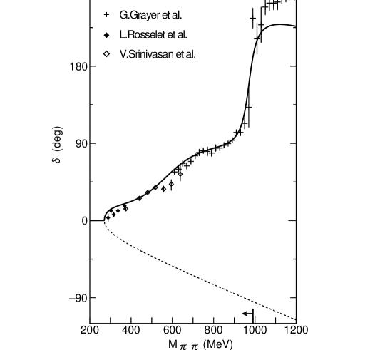
Fig.  2: Fitting of $\delta$ below the $K\overline{K}$ threshold (shown by an arrow) with two resonances. Behavior of the negative background phase is also shown (dashed line). The parameters used are described in the main text. Their best fitted values are listed in Table I.

We first perform a fitting for the $\pi\pi\rightarrow\pi\pi$ phase shift ($\delta$) below the $K\overline{K}$ threshold (280MeV–980MeV). In this region, we suppose the existence of two resonances, $\sigma$ and $f_{0}(980)$, and introduce the negative background mentioned above.

We apply the one-channel two-resonance formula given in Eqs.(2.14), (2.15) and (2.17) with the background phase described in Eqs.(2.21) and (3.1). Necessary parameters to be determined are the following five: $M_{c}(=M_{\scriptscriptstyle(1)})$, $g_{c\pi\pi}(=\stackrel{{\scriptstyle\scriptscriptstyle(1)}}{{g}}_{1})$, $M_{g}(=M_{\scriptscriptstyle(2)})$, $g_{g\pi\pi}(=\stackrel{{\scriptstyle\scriptscriptstyle(2)}}{{g}}_{1})$ and $r_{c}$; $g_{\pi\pi}$ is the coupling constant to $\pi\pi$ channel, where suffix $c$ and $g$ represent $\sigma$ and $f_{0}(980)$, respectively. $r_{c}$ is the “radius” of the negative background. Coupling to $K\overline{K}$ is not needed, because we only treat the phase shift below the threshold here.

The CERN-Münich analysis provides data in the mass region over 600MeV. For acquiring the property of $\sigma$, we supplement the data from the $\pi\pi$ threshold (280MeV) to 600MeV by Srinivasan et al.[28] and by Rosselet et al.[29]

Figure 2 shows the result of our fitting. Values of resonance parameters obtained are listed in Table I. The most notable result is identification of $\sigma$ with the low mass of $553.3\pm 0.5_{st}{\rm MeV}$. According to the result of another fitting to data including those over the $K\overline{K}$ threshold, which will be presented in the next sub-section, the $K\overline{K}$-coupling of $\sigma(555)$ turned out to be negligible. Thus the total width $242.6\pm 1.2_{st}{\rm MeV}$ owes only to its $\pi\pi$ coupling. The fine structure of the phase shift around $280\sim 900$MeV, especially the bump around 750MeV, is reproduced quite well. It is due to the cooperation of the phase increase by $\sigma(555)$ and decrease by the negative background. The radius of the negative background turned out to be $3.46{\rm GeV}^{-1}$.

Table  I: Parameters in the best fit below the $K\overline{K}$ threshold with 2 resonances and the negative background phase. Properties of $f_{0}(980)$ in this table may not be definitive, due to omitting data over the $K\overline{K}$ threshold. For the property of $f_{0}(980)$, see §3.2 and Table II. The value of $g_{K\overline{K}}$ is quoted from the result of fitting data including those over the $K\overline{K}$ threshold. The decay width $\mathchar 28928\relax$ and the “peak width” $\mathchar 28928\relax^{(p)}$ are defined, respectively, as $\mathchar 28928\relax_{i}=\int_{0}^{\infty}ds\mathchar 28928\relax_{i}(s)s^{1/2}\mathchar 28928\relax_{i}^{tot}(s)/(\pi[(s-M_{i}^{2})^{2}+s\mathchar 28928\relax_{i}^{tot}(s)^{2}])$ and $\mathchar 28928\relax_{i}^{(p)}=\mathchar 28928\relax_{i}(s=M_{i}^{2})$. The relation of g and $\mathchar 28928\relax(s)$ is given in our BW formula Eq.(2.14). If we use another form of BW formula, instead of (2.14), as $-M\mathchar 28928\relax(M^{2})/(s-M^{2}+iM\mathchar 28928\relax(M^{2}))$, the pole position is simply given as $s_{pole}/M$=$M-i\mathchar 28928\relax(M^{2})$. See the discussions in §4(A).

	mass(MeV)	$g_{\pi\pi}$(MeV)	$g_{K\overline{K}}/g_{\pi\pi}$	$\mathchar 28928\relax_{tot}({\rm MeV})$=$\mathchar 28928\relax_{\pi\pi}$	$\mathchar 28928\relax^{(p)}({\rm MeV})$
$\sigma$	553.3$\pm$0.5	3336$\pm$12	0.	242.6$\pm$1.2	349.3$\pm$2.5
$(f_{0}(980))$	(970.7$\pm$2.2)	(1768$\pm$24)

	2 BW(${\rm GeV}^{-1}$)
$r_{c}$	3.46$\pm$0.01

3.2. Fitting of $\delta$, $\eta$ and $\phi$ over the $K\overline{K}$ threshold —properties of $f_{0}(980)$

In the following we will investigate the $\pi\pi\rightarrow\pi\pi$ phase shift ($\delta$), the elasticity ($\eta$), and the $\pi\pi\rightarrow K\overline{K}$ phase shift ($\phi$) over the $K\overline{K}$ threshold all together, to study the properties of $f_{0}(980)$. We shall try to fit data in the mass region from 600MeV to 1300MeV with three resonances: $\sigma$, $f_{0}(980)$ and $f_{0}(1300)$. We apply the two-channel three-resonance formula given as Eqs. (2.2.) and (2.2.) with a background phase (2.2.) and (3.1). Thus the total number of parameters is 10: $M_{c}(=M_{\scriptscriptstyle(1)})$, $M_{g}(=M_{\scriptscriptstyle(2)})$, $M_{0}(=M_{\scriptscriptstyle(3)})$, $g_{c\pi\pi}(=\stackrel{{\scriptstyle\scriptscriptstyle(1)}}{{g}}_{1})$, $g_{g\pi\pi}(=\stackrel{{\scriptstyle\scriptscriptstyle(2)}}{{g}}_{1})$, $g_{0\pi\pi}(=\stackrel{{\scriptstyle\scriptscriptstyle(3)}}{{g}}_{1})$, $g_{cK\overline{K}}(=\stackrel{{\scriptstyle\scriptscriptstyle(1)}}{{g}}_{2})$, $g_{gK\overline{K}}(=\stackrel{{\scriptstyle\scriptscriptstyle(2)}}{{g}}_{2})$, $g_{0K\overline{K}}(=\stackrel{{\scriptstyle\scriptscriptstyle(3)}}{{g}}_{2})$ and $r_{c}$.

Data treatment

Fig.  3: The fitting for (a) $\delta$, (b) $\eta$, and (c) $\phi$ over the $K\overline{K}$ threshold with three resonances (fit A: without the two data points (mentioned in the text), fit B: with all data points, fit C: omitting $\phi$ behavior). Data in $600{\rm MeV}\sim 1300{\rm MeV}$ shown by arrow are used for the fitting (the data over 1300MeV are omitted because we must consider the possible effect due to the other resonances in that mass region).

Our treatment of data is as follows:
(a) $\delta$ over 600MeV is quoted from the CERN-Münich analysis.[5] As can be seen in Fig.1, one data point just on the cliff of $f_{0}(980)$ exhibits strange behavior. It looks like a sharp peak, which might not happen in a physical phase shift. Including or excluding this point seriously influences the results on $f_{0}(980)$. Thus we try the following two types of fitting, i.e., one which does not include this data point (fit A) and another which uses all data points (fit B).
(b) $\eta$ is quoted from the same analysis. Also there is a point corresponding to the point referred in (a) just in the narrow dip about 1GeV, which seems to require quite a large inelasticity. In fit A we will not use this point and in fit B we will use it.
(c) $\phi$ is quoted from Ref.?. As can be seen in Fig.3(c), different conflicting results are reported on the $\phi$-behavior. Thus we shall perform a compromised fitting: we use a simple mean of the $\phi$ values by Etkin et al.[30](${\cal E}$) and by Cohen et al.[31](${\cal C}$), a square-mean of their errors as statistical errors, and their differences as systematic errors : $mean=({\cal E}+{\cal C})/2$, $error=\sqrt{(\mathchar 28929\relax{\cal E})^{2}+(\mathchar 28929\relax{\cal C})^{2}}+|{\cal E}-{\cal C}|$.
As will be shown later, our result reproduces that of Etkin et al. rather than that of Cohen et al. The fitting by Morgan and Pennington[7] also exhibits a similar tendency. Our result does not change significantly when using only the data of Etkin et al.

Phase $\delta$ supplied from negative background

Fitting of $\delta$ is shown in Fig.3(a). Concerning our relevant problem, there is no significant difference between the cases in which we use fit A and B.

Note that we have enough space of $\delta$ for 3 resonances: $\sigma$, $f_{0}(980)$ and $f_{0}(1300)$ below 1300MeV, due to the contribution of the negative background. The other resonances, such as a glueball candidate can obviously exist with the mass around $1500\sim 1600{\rm MeV}$.

Table  II: Parameters in the best fit over the $K\overline{K}$ threshold with 3 resonances and the negative background phase. The results on $\sigma$ in this table are somewhat different from those in §3.1, due to omitting the data below 600MeV. This problem is solved in §3.3. For reliable results on $\sigma$, see Table I.  The results on $f_{0}(1300)$ may not be definitive due to the uncertainty in the choice of background phase. See the main text.  On the definition of $\mathchar 28928\relax$ and $\mathchar 28928\relax^{(p)}$, see the caption in Table I.

		mass(MeV)	$g_{\pi\pi}$(MeV)	$g_{K\overline{K}}/g_{\pi\pi}$
$(\sigma)$		(598.6$\pm$15.6-29.6)	(4126$\pm$348)	(0.0$\pm$0.349)
$f_{0}(980)$	fit A	993.2$\pm$6.5$\pm$6.9	1680$\pm$91	1.48$\pm$0.23
	fit B	982.3$\pm$2.2$\pm$2.4	1442$\pm$82	2.82$\pm$0.22
	fit C	987	1947	3.77
$(f_{0}(1300))$		(1313$\pm$36)	(5185$\pm$272)	(0.286$\pm$0.079)

		$\mathchar 28928\relax_{tot}({\rm MeV})$	$\mathchar 28928\relax_{\pi\pi}$	$\mathchar 28928\relax_{K\overline{K}}$
$(\sigma)$		(325.1$\pm$36.3)	(325.1$\pm$36.0)	(0.0$\pm$2.8)
$f_{0}(980)$	fit A	78.3$\pm$11.5	55.70$\pm$6.1	22.7$\pm$9.6
	fit B	114.5$\pm$15.5	46.1$\pm$4.9	68.4$\pm$14.6
	fit C	344	73	272
$(f_{0}(1300))$		(372.0$\pm$34.5)	(355.9$\pm$34.2)	(16.1$\pm$9.9)

		$\mathchar 28928\relax_{tot}^{(p)}({\rm MeV})$	$\mathchar 28928\relax_{\pi\pi}^{(p)}$	$\mathchar 28928\relax_{K\overline{K}}^{(p)}$
$(\sigma)$		(505.0$\pm$89.3)	(505.0$\pm$89.3)	(-)
$f_{0}(980)$	fit A	67.9$\pm$9.4	54.4$\pm$6.1	13.5$\pm$7.4
	fit B	40.5$\pm$4.7	40.5$\pm$4.7	-
	fit C	73.5	73.5	-
$(f_{0}(1300))$		(420.6$\pm$46.2)	(398.6$\pm$44.1)	(22.0$\pm$13.8)

	3 BW(${\rm GeV}^{-1}$)
$r_{c}$	3.76$\pm$0.27

Results on $f_{0}(980)$

The mass of $f_{0}(980)$ is obtained as $993.2\pm 6.5_{st}\pm 6.9_{sys}$MeV(fit A), where the systematic error is estimated as a probable uncertainty ($2\sigma$) of $r_{c}$ (see §3.3).

On the other hand, its coupling to $K\overline{K}$ channel varies a great deal, depending on whether we adopt fit A or B (Table II).

In Fig.3(a) the $\delta$ fitting for fit B is also shown. As can be seen, the fitting over 1GeV is worse than that for fit A, due to the influence of the data point on the cliff, referred to above.

The elasticity plots for fit A and B are shown in Fig.3(b). If we take the point on the cliff into account (fit B), the fitted curve of the elasticity passes through the lower region, and the $\phi$-fitting becomes slightly worse (Fig.3(c)). Thus the $K\overline{K}$ width and the total width in fit B must be larger than those in case of fit A, respectively. If we intend to reproduce that point exactly, the $K\overline{K}$ width and total width become 272MeV and 344MeV, respectively (fit C). They seem to be consistent with recent values obtained by Zou et al.[10] But in this case it is difficult to reproduce the $\phi$ behavior as shown in the figure. The obtained width of $f_{0}(980)$ without this point (fit A) is $78.3\pm 11.5_{st}$MeV, which is consistent with a value given by Morgan and Pennington. [7]

It should be noted that the results on properties of $f_{0}(1300)$ in Table II are not definitive, because they strongly depend on how to choose the background phase, and also on the properties of other possible $f_{0}$ with higher masses.

3.3. Fitting for the entire relevant mass region — possible form of negative background

As was mentioned in the previous two sub-sections, some differences of the obtained results between the fittings in the different mass regions suggest that the shape of background phase is not as simple as Eq.(3.1).

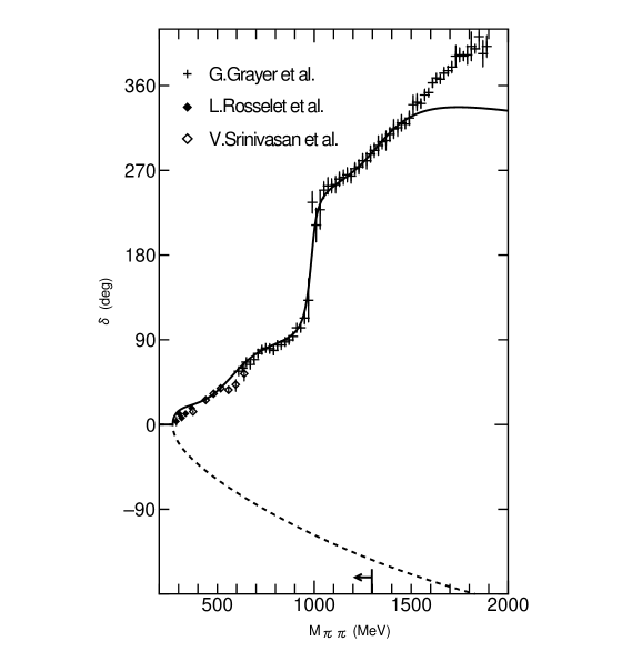
Fig.  4: Fitting for $\delta$ through entire mass region with “soft” repulsive core. The parameters used for $\sigma$ are quoted from Table I, while those for $f_{0}(980)$ and $f_{0}(1300)$ are from Table II (fit A).

From a consideration on the origin of negative background, considering an analogy with the case of nucleon-nucleon interactions (to be given in §4(C)), we consider it reasonable that the radius of the negative background $r_{c}$ becomes smaller with the increase of the pion momentum. Thus we shall further try another type of fitting through the whole relevant mass region to determine a possible shape of the background:
(a) We will introduce an exponentially decreasing factor to the radius of the background $r_{c}$ (Eq.(3.1)),

$$r_{c}\rightarrow r_{c}exp(-b|{\bf P}_{\pi\pi}|),$$

(3.2)

where the parameter $b$ also has dimensions of length.
(b) Parameters giving the properties of three resonances are fixed, i.e., those for $\sigma$ are taken from the values obtained from fitting below the $K\overline{K}$ threshold, while those for $f_{0}(980)$ and $f_{0}(1300)$ are from the values over the threshold.

The result of fitting is shown in Fig.4, where the best fit parameters of the background core are given in Table III. The fitting looks quite good through the entire relevant mass region.

Table  III: Parameters in the best fit for the core of Eq.(3.2).

$r_{c}({\rm GeV}^{-1})$	$b({\rm GeV}^{-1})$
5.36$\pm$0.01	0.480$\pm$0.009

3.4. Remarks on the method of our analysis

In performing the analysis in this section we have actually applied an analytically discontinued (A.D.) density matrix, whose elements have non-zero values only over the threshold of the corresponding channel as

$$\rho = diag(\frac{|{\bf p}_{1}|}{8\pi\sqrt{s}},\frac{|{\bf p}_{2}|}{8\pi\sqrt{s}}),$$

$$|{\bf p}_{1}| = \sqrt{\frac{s}{4}-m_{\pi}^{2}}\theta(s-4m_{\pi}^{2}),\ |{\bf p}_{2}|=\sqrt{\frac{s}{4}-m_{K}^{2}}\theta(s-4m_{K}^{2})$$ (3.3)

(correspondingly in fitting of §3.1 below the $K\overline{K}$ threshold we have applied the one-channel formula, and in fitting of §3.2 applied the two-channel formula, since only the $|{\bf p}_{1}|$ remains non-zero for the region below the $K\overline{K}$ threshold).

Thus the resonance parameters obtained in this analysis are considered to represent the particle properties in the zero-th approximation, which are determined only through the quark-gluon color-confining dynamics, omitting the “residual” strong interactions among color-singlet hadrons. However, this treatment violates the “sacred” requirement of analyticity of the scattering amplitude. Applying an analytically continued (A.C.) density matrix is considered to take into account the effects of virtual $\pi\pi$ and $K\overline{K}$ channels in extracting the resonant-particle properties.

We have estimated these effects, actually applying the A.C. density matrix: The result of re-analysis of data (including all of $\delta$, $\eta$, and $\phi$) in the region 600$\leq$$\sqrt{s}$$\leq$1300MeV produces little change in the properties of $\sigma(555)$ and $f_{0}(980)$. This seems to be due to the zero coupling of $\sigma$ to the $K\overline{K}$ channel (cf. Table I) and the small width of $f_{0}$. Then, in order to estimate the effects on the $\sigma$-properties by applying the A.C. density matrix for $f_{0}$, we have performed fitting under the $K\overline{K}$ threshold by taking the $f_{0}$ properties as obtained above and by setting $g_{K\overline{K}}(\sigma)$=0. The results are $M_{\sigma}$=568.9$\pm$0.5MeV and $\mathchar 28928\relax_{\sigma}$=250.5$\pm$3.7MeV. The small differences between these values and those in the case with A.D. density matrix (Table I) owe to the A.C. effect on $f_{0}$, which has non-zero coupling to $K\overline{K}$.

In the analysis of this section we have not taken into account the Adler-zero condition[32] for the amplitude: The possible effects of this requirement on the properties of $\sigma$ and of $f_{0}$ are considered to be small, although it may affect the values of parameters relevant to the energy region near the $\pi\pi$-threshold.

Here we should point out that it is generally very difficult to take quantitatively the effects of strong interaction into account, since hadrons are interacting “democratically” among various possible channels (remember the long history of strong interactions before QCD). Also we feel that the physical backgrounds of the analyticity of the scattering amplitude in the level of point-like hadrons should be re-examined presently, when the “global” properties of hadrons are determined through the confinement dynamics of the quark-gluon world and the hadrons have space-time extensions.

4 Physical implications of our results and related problems

(A) Relation of the IA method to the other approaches

The $S$-matrix must satisfy the unitarity (Eq.(2.4)) and be symmetric due to time reversal invariance (Eq.(2.5)). The corresponding conditions (2.8) and (2.9) are imposed on the ${\cal T}$ matrix, and there have appeared various methods[33] to parametrize the general solutions satisfying these conditions.

In the most conventional ${\cal K}$ matrix methods[7, 8] the ${\cal T}$ matrix is first represented by the ${\cal K}$ matrix as

$${\cal T}={\cal K}\frac{1}{1+i\rho{\cal K}}$$ (4.1)

and is regarded as an analytic function on the Riemann sheets of complex $s$-variable, except for the right and left hand singularities and the poles. Then the ${\cal T}$ matrix for any real symmetric ${\cal K}$ matrix automatically satisfies the unitarity and the time reversal invariance.

Our relevant problem is to find pole positions of the ${\cal T}$ matrix, which are related to the masses and the decay widths of resonant particles.

However, the parameters used in the ${\cal K}$ matrix are not directly related to these properties of physical particles, and there seem to be many unpleasant features: Even the number of ${\cal T}$ matrix poles is determined by the choice of the ${\cal K}$ matrix parametrization. Moreover, the contributions to the ${\cal T}$ matrix of the resonances and the non-resonant background cannot be separated in the simple ${\cal K}$ matrix representation. In the Dalitz-Tuan representation[34] of the ${\cal T}$ matrix, which is obtained by modifying the ${\cal K}$ matrix representation, the background and resonance contributions are clearly separated, and the parametrization used in Ref.? is equivalent to our Eq.(2.2.) in the one-resonance case.

On the other hand, in the $\omega$-method which was proposed by Kato[35] and by Fujii and Fukugita,[6] the pole positions of the $S$-matrix are directly parametrized on complex Riemann sheets. They use the Le-Counter Newton equation for the $S$ matrix in two-channel case,

$$S_{ii} = {\bf d}^{(i)}(s)/{\bf d}(s)\ \ {\rm for}\ i=1,2,$$

$$S_{11} S_{22} -S_{12}^{2}={\bf d}^{(1,2)}(s)/{\bf d}(s).$$ (4.2)

Here ${\bf d}(s)$, defined on the physical Riemann sheet $I$, includes the right hand singularities, while the ${\bf d}^{(1)}(s)$, ${\bf d}^{(2)}(s)$ and ${\bf d}^{(1,2)}(s)$ are the analytic continuations of ${\bf d}(s)$ in the sheet II, IV and III, obtained by the change of signs of momenta $p_{1}\rightarrow-p_{1}$, $p_{2}\rightarrow-p_{2}$ and $(p_{1},p_{2})\rightarrow(-p_{1},-p_{2})$. The four Riemann sheets are mapped onto the single $\omega$-plane[35]

$$\omega=\frac{1}{\sqrt{m_{K}^{2}-m_{\pi}^{2}}}(p_{1}+p_{2}).$$ (4.3)

The poles of the $S$ matrix correspond to the zeros of ${\bf d}(s)$ in the $\omega$-plane. The Breit Wigner resonance formula is obtained with ${\bf d}(s)$

$${\bf d}(s)=\frac{m_{K}^{2}-m_{\pi}^{2}}{\omega^{2}}(\omega-\omega_{r})(\omega+\omega_{r}^{*})(\omega-\omega_{s})(\omega+\omega_{s}^{*}),$$ (4.4)

where the four zeros ($\omega_{r}$, $\omega_{s}$ and their inversion for the imaginary axis $-\omega_{r}^{*}$, $-\omega_{s}^{*}$) satisfy certain constraints from the unitarity. Then, ${\bf d}(s)$ becomes equal to $\stackrel{{\scriptstyle\scriptscriptstyle(i)}}{{d}}(s)$ in Eq.(2.38), if we replace $\sqrt{s}\mathchar 28928\relax_{i}(s)\equiv\sqrt{s}\frac{p_{i}}{8\pi s}g_{i}^{2}$ by $m\mathchar 28928\relax_{i}^{\prime}(s)\equiv m\frac{p_{i}}{8\pi m^{2}}g_{i}^{2}$, and the final form of the $S$ matrix in Eq.(4.2) coincides with our Eq.(2.39).

In our case with $\sqrt{s}\mathchar 28928\relax_{i}(s)$ the $S$-matrix has six poles. Since the $S$-matrix in the IA-method is described by the simple Breit Wigner resonance formulae and is parametrized directly in terms of the masses and coupling constants, it seems to us not necessary to determine the pole positions of $S$-matrix which have no direct physical meanings.

(B) Central production of $\sigma(555)$

According to Watson’s final state interaction theorem, the phase of production amplitude of all types of $\pi\pi$ production processes is determined through the $\pi\pi$-scattering amplitude. Accordingly, if the existence of $\sigma(555)$ is really observed in the $\pi\pi$-scattering, the corresponding signal must also be observed in any production processes.

In the observations of the $\pi\pi$ production in $pp$ central collision: $pp\rightarrow p_{f}(\pi\pi)p_{s}$ with hundreds of GeV/c momentum incident proton beam, a huge event concentration around $m_{\pi\pi}=0.3\sim 1{\rm GeV}$ has been clearly seen. [36, 37, 38] In the conventional treatment thus far made, this was regarded as a simple “background”.

However, we find[22] that the $f_{0}(980)$ peak slides down around 900MeV, probably due to “destructive” interference with the concentration. We have performed a fitting with two Breit-Wigner resonances ($f_{0}(980)$ and another of lower mass and wide width), and found that “destructive” interference occurs with a relative phase between the two resonances, which seems to be consistent with the above theorem. This fact supports our interpretation of this concentration being due to production of $\sigma(555)$. However, it is to be noted that the mass and the width obtained in Ref.? may not be definitive, and the above result should be checked further. An exact analysis on the $pp$ central collision will be reported soon.[39]

Moreover, by comparing the $\pi\pi$-spectra in the $pp$ central collisions and in the peripheral $\pi^{-}p$ charge-exchange processes, it is seen that the production probability of $\sigma(555)$ in the former may be larger than that in the latter. This fact seems to be explicable by supposing that $\sigma(555)$ is a member of the new type scalar nonet, which will be discussed in (D) below.

(C) “Repulsive core” in $\pi\pi$-interactions

Table  IV: The value of hard core radius of $\pi\pi$ interactions, in comparison with the cases of $\alpha$-$\alpha$ and $N$-$N$ interactions. Structural sizes (EM r.m.s radii) of relevant particles are also shown.   * value from Table II.  ** value of soft core from Table III. A permissible minimum of the $\pi\pi$ core radius turned to be 0.5fm ($2.5{\rm GeV}^{-1}$) (see the text).

system	$r_{c}$	$\sqrt{<r^{2}>}$
$\alpha-\alpha$	$2fm$	$1.6{\rm fm}$
	$(10{\rm GeV}^{-1})$
$N$-$N$	$0.4\sim 0.5{\rm fm}$	$0.8{\rm fm}$
	$(2\sim 2.5{\rm GeV}^{-1})$
$\pi-\pi$	$0.68{\rm fm}$	$0.7{\rm fm}$
	$(3.46{\rm GeV}^{-1})^{*}$
	$1.06{\rm fm}$
	$(5.36{\rm GeV}^{-1})^{**}$

In our analysis of the $\pi\pi$-scattering phase shift of §3, leading to strong evidence for the existence of $\sigma(555)$, introduction of a negative-phase background Eq.(3.1) has played a crucial role. We consider that a possible physical origin of this background is of a very fundamental nature and that a corresponding repulsive force may be reflecting a Fermi-statistics nature of constituent quarks and anti-quarks of pions in the $\pi\pi$-system: A repulsive force due to a similar mechanism has been known since long ago to exist in nucleus-nucleus interactions. In the $\alpha$-$\alpha$ system it is phenomenologically known that there exists a strong short-range repulsion [40, 41, 42, 43] which gives a negative scattering phase shift of the same form as Eq.(3.1) with a corresponding size of core $r_{c}^{\alpha\alpha}=2{\rm fm}$ (, while the r.m.s. radius, a “structural size”, of $\alpha$ is $\sqrt{<r^{2}>_{\alpha}}=1.6{\rm fm}$). The physical origin of this repulsion was explained to be [40] due to the Fermi-statistics property of constituent nucleons of each $\alpha$-nucleus in the $\alpha$-$\alpha$ system. Then it may be reasonable to imagine, [43, 44, 45] by replacing the constituent nucleons in the $\alpha$-particle with constituent quarks in the nucleon, that there may exist a strong short-range repulsion in nuclear forces between nucleon-nucleon system. Actually it has been shown [46, 47, 48] phenomenologically that there surely exists a strong repulsive core in ${}^{1}S_{0}$ states. Extensive investigations[49] on nuclear forces have been done by many physicists, and the size of the corresponding hard core radius was reported to be $r_{c}^{NN}=0.4\sim 0.5{\rm fm}$, while the electromagnetic (EM) r.m.s. radius of the proton is $\sqrt{<r^{2}>_{p}}=0.8{\rm fm}$. A formulation [50] to derive the short range part of the $N$-$N$ interaction directly from the quark-quark interaction has also been given.

Now it seems to us quite natural that a possible physical origin of our repulsive core in the $\pi\pi$ iso-singlet $S$-wave state is the same mechanism as that in the nuclear force. Actually an interesting work from this viewpoint has been done by Ref.?. The values of our hard core radii in the $\pi\pi$ interaction are collected in Table IV with EM r.m.s. radius of the pion, in comparison with the mentioned cases of the $\alpha$-$\alpha$ and the $N$-$N$ interactions.

Hard core radii in the respective cases may be directly related with and may have similar orders of magnitude to the structural sizes of corresponding composite particles, considering our relevant mechanism. This expectation seems to be realized, as is seen in Table IV.

However, one may feel that $r_{c}^{\pi\pi}$ seems to be rather large. We have made some analysis on this point. To reproduce the characteristic phase shift below $K\overline{K}$ threshold, a certain magnitude of the core radius is required. A permissible minimum value of the radius may be $2.5{\rm GeV}^{-1}$.

Here it is noted that our analysis with the “soft-core” background Eq.(3.2) has been stimulated by the corresponding one [52] in the case of nuclear force.

We have also estimated the $\pi\pi$ scattering length $a_{len}$=$a_{len}^{\sigma}$-$r_{c}$ using the properties of $\sigma$ in Table I and the values of $r_{c}$ from both in Tables I and III. (We have used the form of relativistic B.W. formula, Eq.(2.14), in order to estimate $a_{len}^{\sigma}$.) The results are given in Table V in comparison with the other estimations, which seem to be mutually consistent. However, we note that the values of $a_{len}^{\sigma}$ depend largely upon the form of the relativistic B.W. formula, and effects due to various possible effects of hadron interactions (see §3.4.).

Table  V: Scattering length obtained from our fitting, in comparison with other estimations.

Our estimation	0.69fm ($r_{c}$=0.68fm)
$a_{len}$=$a_{len}^{\sigma}$-$r_{c}$	0.32fm ($r_{c}$=1.06fm)
Other estimation	0.37$\pm$0.07fm [29][53]
	0.34$\pm$0.13fm [54]
Current Algebra	$a_{len}$=$\frac{7}{32\pi}\frac{m_{\pi}}{f_{\pi}^{2}}$
(Non-linear $\sigma$ model)	=0.22fm[55, 56]

(D) Possible existence of chiralons; new scalar and axial-vector meson nonets

Classification of mesons usually follows the $LS$-coupling scheme of the non-relativistic quark model. We generalized it covariantly, keeping good $L$ and $S$ quantum numbers, to the boosted $LS$-coupling scheme.[57] In this scheme, the Bargmann-Wigner spinor wave function, which is a covariant generalization of Pauli spin functions, implies that the constituent quark and anti-quark are in “parton-like” parallel motion[58], i.e., they move with the same velocity as that of the meson. “Usual” scalar and axial meson nonets can be classified in the first $L$-excited state in this scheme.

On the other hand, in most ENJL models,[2] as a low energy effective theory of QCD, there exist four chiral symmetric nonets with $J^{PC}$= $0^{++}$, $0^{-+}$, $1^{--}$ and $1^{++}$. In ENJL essentially only local composite quark and anti-quark operators are treated, thus missing $L$-excited states in principle. Here it is to be noted that the constituent quark and antiquark inside of these $0^{++}$ and $1^{++}$ nonets are shown mutually in an anti-parallel motion. Members of these nonets are apparently different from the above-mentioned Bargmann-Wigner particles

Accordingly, it seems to us that, in order to complete the meson spectroscopy, we must take these extra “ultra-relativistic” $0^{++}$ and $1^{++}$ nonets into account, in addition to the “non-relativistic” ones described by the $LS$ coupling scheme. We call these “chiralons”.[59]

It is expected that production of chiralons will be enhanced in $pp$ central collisions, where constituent valence quarks and sea-antiquarks in anti-parallel motion exist. Thus if we assume that $\sigma$ is a member of scalar chiralons, enhancement of $\sigma$ in central collisions, mentioned in (B), may be clearly explained.

The $f_{0}(1300)$ given in our analysis in §3 may be assigned to a member of the normal $0^{++}$ nonet in the ${}^{3}P_{0}$ $q\overline{q}$ state. Also we are examining the possibility of $f_{0}(980)$ being a hybrid meson with a massive constituent gluon.[60]

Finally we would like to note that one of the authors has examined [61] recently the properties of $\sigma(555)$, obtained in this work, from the viewpoint of the effective chiral Lagrangian of the linear $\sigma$-model, and shown that $\sigma(555)$ may be identified with the chiral partner to the Nambu-Goldstone $\pi$-meson.

5 Summary

In this paper we have re-analyzed the phase-shift between the $\pi\pi$-threshold and 1300${\rm MeV}$ by applying a newly developed IA-method. The results are summarized as follows:
(1) The $\pi\pi\rightarrow\pi\pi$ phase shift has been analyzed in the mass region of the $\pi\pi$- to the $K\overline{K}$- thresholds, giving strong evidence for the existence of $\sigma$, with mass of $553.3\pm 0.5_{st}{\rm MeV}$ and width of $242.6\pm 1.2_{st}{\rm MeV}$.
(2) Our best fit value of a radius of the repulsive core in $\pi\pi$ interactions, whose introduction is the keystone for leading to the existence of $\sigma(555)$, is $3.5{\rm GeV}^{-1}$ (in case of “hard core”)/$5.4{\rm GeV}^{-1}$ (“soft core”). This value is almost equal to the structural size of the pion ($3.5{\rm GeV}^{-1}$). This situation is quite similar in the case of $N$-$N$ interactions, giving support to our interpretation of the repulsive core.
(3) The properties of $f_{0}(980)$ have been investigated from the data including those over the $K\overline{K}$ threshold. The mass is obtained as $993.2\pm 6.5_{st}\pm 6.9_{sys}{\rm MeV}$. Its total width varies due to the uncertainty of $K\overline{K}$ coupling, to be $78.3\pm 11.5_{st}{\rm MeV}$ (fit A), $114.5\pm 15.5_{st}{\rm MeV}$ (fit B) or $344{\rm MeV}$ (fit C), corresponding to the three different treatments of the elasticity and the $\pi\pi\rightarrow K\overline{K}$ phase shift, both of which have large experimental uncertainties. However, fit C has difficulty to reproduce the experimental $\pi\pi\rightarrow K\overline{K}$ phase behavior.

References

- [1] Y. Nambu and G. Jona-Lasinio,Phys. Rev. 122 (1961), 345.
- [2] T.Eguchi and H.Sugawara, Phys. Rev. D 10 (1974), 4257. H.Kleinert, Lecture at Erice Summer School of Subnuclear Physics, Erice, Italy (1976); Phys. Lett. B 59 (1975), 163; Phys. Lett. B 62 (1976), 429. G.Konishi, T.Saito and K.Shigemoto, Phys. Rev. D 13 (1976), 3327. A.Chakrabarti and B.Hu, Phys. Rev. D 13 (1976), 2347. P.D.Mannheim, Phys. Rev. D 14 (1976), 2027; D 15 (1977), 549. T.Kugo, Prog. Theor. Phys. 55 (1976), 2032. K.Kikkawa, Prog. Theor. Phys. 56 (1976), 947. T.Eguchi, Phys. Rev. D 14 (1976), 2755. C.M.Bender, F.Cooper and G.S.Guralnik, Ann. of Phys. 109 (1977), 165. K.Shizuya, Phys. Rev. D 21 (1980), 2327. D.Ebert and M.K.Volkov, Z. Phys. C 16 (1983), 205. M.K.Volkov, Ann. of Phys. 157 (1984), 282.
- [3] M.Taketani et al., Prog. Theor. Phys. Suppl. No.39 (1967), Chapter 3 (S.Ogawa et al., p.140).
- [4] S.Furuichi, H.Kanada and K.Watanabe, Prog. Theor. Phys. 64 (1980), 959.
- [5] G.Grayer et al., Nucl. Phys. B 75 (1974), 189. B.Hyams et al., Nucl. Phys. B 64 (1973), 134.
- [6] Y.Fujii and M.Fukugita, Nucl. Phys. B 85 (1975), 179.
- [7] K.L.Au, D.Morgan and M.R.Pennington, Phys. Rev. D 35 (1987), 1633. D.Morgan and M.R.Pennington, Phys. Rev. D 48 (1993), 1185.
- [8] V.V.Anisovich, A.A.Kondashov, Yu.D.Prokoshkin, S.A.Sadovsky and A.V.Sarantsev, Phys. Lett. B 355 (1995), 363.
- [9] E.Beveren et al., Z. Phys. C 30 (1986), 615.
- [10] B.S.Zou and D.V.Bugg, Phys. Rev. D 48 (1993), R3948. B.S.Zou and D.V.Bugg, Phys. Rev. D 50 (1994), 591.
- [11] N.A.Törnqvist, Z. Phys. C 68 (1995), 647.
- [12] M.Gell-Mann and M.Lvi, Nuovo Cim. 16 (1960), 705.
- [13] T.H.R.Skirme, Proc. Roy. Soc. London Ser. A260 (1961), 127; Nucl. Phys. 31 (1962), 556.
- [14] T.Kunihiro, Prog. Theor. Phys. Suppl. No.120 (1995), 75.
- [15] G.Mennessier, Z. Phys. C 16 (1983), 241. S.Minami, Prog. Theor. Phys. 81 (1989), 1064.
- [16] M.Svec, A de Lesquen and L.van Rossum, Phys. Rev. D 46 (1992), 949.
- [17] H.Shimizu, contributed paper on Particle and Nuclei XIII International Conference -PANIC XIII, Perugia, Italy, June 1993.
- [18] R.Kamiski, L.Leniak and J.-P.Maillet, Phys. Rev. D 50 (1994), 3145.
- [19] R.Delbourgo and M.D.Scadron, Phys. Rev. Lett. 48 (1982), 379. V.Elias and M.D.Scadron, Phys. Rev. Lett. 53 (1984), 1129; Mod. Phys. Lett. A10 (1995), 251.
- [20] T.Hatsuda and T.Kunihiro, Prog. Theor. Phys. 74 (1985), 765; Phys. Rep. 247 (1994), 221; T.Kunihiro and T.Hatsuda, Phys. Lett. B 206 (1988), 385.
- [21] S.Klimt, M.Lutz, U.Vogl and W.Weise, Nucl. Phys. A516 (1990), 429.
- [22] T.Ishida et al., KEK-Preprint 95-159 (1995); a paper of GAMS collaboration is under preparation.
- [23] Review of Particle Properties, Rev. Mod. Phys. 48 Part II S114 (1976).
- [24] F.Binon et al., Nuovo Cim. 78A (1983), 313. D.Alde et al., Nucl. Phys. B 269 (1986), 485.
- [25] V.V.Anisovich et al., Phys. Lett. B 323 (1994), 233.
- [26] S.Ishida, talk presented at Gluonium’95. K.Yamada, talk presented at HADRON’95, Nihon Univ. Preprint NUP-A-95-14 (1995).
- [27] See, for example, C.A.Heusch, QCD 20 Years Later, ed. P.M.Zerwas and H.A. Kastrup (World Scientific, 1992), p.555.
- [28] V.Srinivasan et al., Phys. Rev. D 12 (1975), 681.
- [29] L.Rosselet et al., Phys. Rev. D 15 (1977), 574.
- [30] A.Etkin et al., Phys. Rev. D 28 (1982), 1786.
- [31] D.Cohen et al., Phys. Rev. D 22 (1980), 2595.
- [32] S.L.Adler, Phys. Rev. 139B (1965), 1638.
- [33] A.M.Badalyan, L.P.Kok, M.I.Polikarpov and Yu.A.Simonov, Phys. Rep. 82 (1982), 31.
- [34] R.H.Dalitz and S.Tuan, Ann. of Phys. 10 (1960), 307.
- [35] M.Kato, Ann. of Phys. 31 (1965), 130.
- [36] T.Akeson et al., Nucl. Phys. B 264 (1986), 154.
- [37] A.Breakstone et al., Z. Phys. C 31 (1986), 185; Z. Phys. C 48 (1990), 569.
- [38] T.A.Armstrong et al., Z. Phys. C 51 (1991), 351.
- [39] S.Ishida, M.Y.Ishida, H.Takahashi, T.Ishida, K.Takamatsu and T.Tsuru, in preparation.
- [40] H.Margenau, Phys. Rev. 59 (1941), 37.
- [41] O.Endo, I.Shimodaya and J.Hiura, Prog. Theor. Phys. 31 (1964), 1157.
- [42] P.Darriulat et al., Phys. Lett. 11 (1964), 326.
- [43] I.Shimodaya, R.Tamagaki and H.Tanaka, Prog. Theor. Phys. 27 (1962), 793.
- [44] S.Otsuki, R.Tamagaki and M.Wada, Prog. Theor. Phys. 32 (1964), 220.
- [45] S.Machida and M.Namiki, Prog. Theor. Phys. 33 (1965), 125.
- [46] R.Tastrow, Phys. Rev. 79 (1950), 389; Phys. Rev. 81 (1951), 165.
- [47] J.Iwadare, S.Otsuki, R.Tamagaki and W.Watari, Prog. Theor. Phys. 16 (1956), 472; Prog. Theor. Phys. Suppl. No.3 (1956) 32.
- [48] H.P.Stapp, T.J.Ypsilantis and N.Metropolis, Phys. Rev. 105 (1957), 302.
- [49] M.Taketani et al., Prog. Theor. Phys. Suppl. No.39 (1967); No.42 (1968). In particular see Chapter 7 (S.Otsuki, No.42, p.39) and also Chapter 6 (N.Hoshizaki, No.42, p.1).
- [50] V.G.Neudatchin, Yu.F.Smirnov and R.Tamagaki, Prog. Theor. Phys. 58 (1977), 1072. M.Oka and K.Yazaki, Prog. Theor. Phys. 66 (1981), 556, 572.
- [51] K.Holinde and M.B.Johnson, Phys. Lett. B 144 (1984), 163.
- [52] R.Tamagaki, M.Wada and W.Watari, Prog. Theor. Phys. 33 (1965), 55.
- [53] M.N.Nagels et al., Nucl. Phys. B 147 (1979), 189.
- [54] A.A.Bel’kov et al., JETP Lett. 29 (1979), 597.
- [55] S.Weinberg, Phys. Rev. Lett. 17 (1966), 616.
- [56] B.W.Lee and H.T.Nieh, Phys. Rev. 166 (1968), 1507. S.Gasiorowicz and D.A.Geffen, Rev. Mod. Phys. 41 (1969), 531.
- [57] S.Ishida and M.Oda, Proc. of Int. Symp. on Extended Objects and Bound Systems, Karuizawa JAPAN, ed. O.Hara, S.Ishida and S.Naka (World Scientific, 1992), p.181.
- [58] S.Ishida, M.Y.Ishida and M.Oda, Prog. Theor. Phys. 93 (1995), 939.
- [59] S.Ishida and M.Y.Ishida, in preparation.
- [60] S.Ishida, H.Sawazaki, M.Y.Ishida, K.Yamada, T.Ishida, T.Kinashi, K.Takamatsu and T.Tsuru, talk presented at HADRON’95, Nihon Univ. Preprint NUP-A-95-15, KEK Preprint 95-167 (1995).
- [61] M.Y.Ishida, Univ. of Tokyo preprint UT-745 (1996).