UMN-TH-1515/96

hep-ph/9610319

October 1996

A BIG BANG NUCLEOSYNTHESIS LIKELIHOOD ANALYSIS
OF THE BARYON-TO-PHOTON RATIO AND
THE NUMBER OF LIGHT PARTICLE DEGREES OF FREEDOM

Keith A. Olive

University of Minnesota, School of Physics and Astronomy

116 Church St SE, Minneapolis, MN 55455

David Thomas

University of Florida, Dept. of Physics

Box 118440, Gainesville, FL 32611-8440

Abstract

We extend the model-independent likelihood analysis of big bang nucleosynthesis (BBN) based on ⁴He and ⁷Li to allow for numbers of degrees of freedom which differ from the standard model value characterized by $N_{\nu}=3$. We use the two-dimensional likelihood functions to simultaneously constrain the baryon-to-photon ratio and the number of light neutrinos. The upper limit thus obtained is $N_{\nu}<4.0$ (at 95% C.L.). We also consider the consequences if recent observations of deuterium in high-redshift QSO absorption-line systems (QSOALS) are confirmed.

1 Introduction

In recent years the comparison between standard big bang nucleosynthesis and observational data on elemental abundances has come under close scrutiny. Minor changes in the theoretical abundances (improvements in the code, updated neutron lifetime data) combined with many new determinations of the abundances of the light element isotopes, D, ³He, ⁴He, and ⁷Li have led to a flurry of sophisticated statistical analyses of BBN [1, 2, 3, 4, 5, 6, 7, 8]. The results of these analyses however depend strongly on the assumptions made about galactic chemical evolution, and in particular, the chemical evolution of deuterium. For the most part, the comparison between BBN theory and the observational data made heavy use of the solar value of D + ³He because it provided a (relatively large) lower limit for the baryon-to-photon ratio [9], $\eta_{10}\equiv 10^{10}\eta>2.8$. This limit for a long time was seen to be essential because it provided the only means for bounding $\eta$ from below and in effect allows one to set an upper limit on the number of neutrino flavors [10], $N_{\nu}$, as well as other constraints on particle physics properties. The upper bound to $N_{\nu}$ is in fact strongly dependent on the lower bound to $\eta$. For lower $\eta$ the ⁴He abundance predicted by BBN drops, allowing for a larger $N_{\nu}$ to match a given primordial ⁴He abundance, $Y_{\rm p}$, as determined from the observations. For $\eta<4\times 10^{-11}$, there is no bound whatsoever on $N_{\nu}$ [11].

It was argued [9] that since stars (even massive stars) do not destroy ³He in its entirety, we can obtain a bound on $\eta$ from an upper bound to the solar D and ³He abundances. One can in fact limit [9, 12] the sum of primordial D and ³He by applying the expression below at $t=\odot$

$${\rm\left({D+\hbox{${}^{3}$He}\over H}\right)_{p}\leq\left({D\over H}\right)_{t}}+{1\over g_{3}}{\rm\left({\hbox{${}^{3}$He}\over H}\right)_{t}}$$ (1)

In (1), $g_{3}$ is the fraction of a star’s initial D and ³He which survives as ³He. For $g_{3}>0.25$ as suggested by standard stellar models, and using the solar data on D/H and ³He/H, one finds $\eta_{10}>2.8$. This argument has been improved recently [13] ultimately leading to a stronger limit [6] $\eta_{10}>3.8$ and a best estimate $\eta_{10}=6.6\pm 1.4$. The stochastic approach used in [14] could only lower the bound from 3.8 to about 3.5 when assuming as always that $g_{3}>0.25$.

The limit $\eta_{10}>2.8$ derived using (1) is really a one shot approximation. Namely, it is assumed that material passes through a star no more than once. However, to determine whether or not the solar (and present) values of D/H and ³He/H can be matched to a given primordial abundance, it is necessary to consider models of galactic chemical evolution. In the absence of stellar ³He production, particularly by low mass stars, it was shown [15] that there are indeed suitable choices for a star formation rate and an initial mass function to: 1) match the D/H evolution from a primordial value (D/H)${}_{\rm p}=7.5\times 10^{-5}$, corresponding to $\eta_{10}=3$, through the solar and present interstellar medium (ISM) abundances, while 2) at the same time keeping the ³He/H evolution relatively flat so as not to overproduce ³He at the solar and present epochs. This was achieved for $g_{3}>0.3$.

In the context of models of galactic chemical evolution, there is, however, little justification a priori for neglecting the production of ³He in low mass stars. Indeed, stellar models predict that considerable amounts of ³He are produced in stars between 1 and 3 M_⊙ [16] and this prediction is consistent with the observation of high ³He/H in planetary nebulae [17]. Generally, implementation of these ³He yields in chemical evolution models leads to a gross overproduction of ³He/H particularly at the solar epoch [18].

As indicated earlier, the presence of a lower bound on $\eta$ allows us to place an upper bound to the number of neutrino flavors. From (1), the limit $\eta_{10}>2.8$ corresponds to the limit $N_{\nu}<3.3$ [19]. However, it should be noted that for values of $\eta_{10}$ larger than 2.8, the central or best-fit value for $N_{\nu}$ is closer to 2 [20, 3, 6] and the upper bound is actually found to be much smaller with a careful treatment of the uncertainties, $N_{\nu}\mathrel{\mathchoice{\lower 3.6pt\vbox{\halign{$\mathsurround=0pt\displaystyle\hfil#\hfil$\cr<\crcr\sim\crcr}}}{\lower 3.6pt\vbox{\halign{$\mathsurround=0pt\textstyle\hfil#\hfil$\cr<\crcr\sim\crcr}}}{\lower 3.6pt\vbox{\halign{$\mathsurround=0pt\scriptstyle\hfil#\hfil$\cr<\crcr\sim\crcr}}}{\lower 3.6pt\vbox{\halign{$\mathsurround=0pt\scriptscriptstyle\hfil#\hfil$\cr<\crcr\sim\crcr}}}}3.1$ [20, 3], though this limit is relaxed somewhat when the distribution for $N_{\nu}$ is renormalized [21]. The range in $\eta_{10}$ of $6.6\pm 1.4$, corresponds to an even tighter limit on $N_{\nu}=2.0\pm 0.3$ [6] and indicates a problem when trying to make use of D and ³He in conjunction with ⁴He.

Given the magnitude of the problems concerning ³He [18], it would seem unwise to make any strong conclusion regarding big bang nucleosynthesis which is based on ³He. In addition, deuterium is highly sensitive to models of chemical evolution. Values of primordial D/H as high as $2\times 10^{-4}$ (i.e. as determined in some measurements of D/H in quasar absorption systems [22]) were shown to be viable in models of chemical evolution and consistent with other observational constraints [23]. For these reasons it was argued [7, 8] that the analysis comparing BBN theory and observations should be based primarily on the two isotopes which are the least sensitive to the effects of evolution, namely, ⁴He and ⁷Li.

In [8], the baryon-to-photon ratio, $\eta$ was determined on the basis of a likelihood analysis using ⁴He and ⁷Li. Because of the monotonic dependence of ⁴He on $\eta$, the ⁴He likelihood distribution has a single (but relatively broad) peak at $\eta_{10}=1.75$. ⁷Li, on the other hand, is not monotonic in $\eta$, the BBN prediction has a minimum at $\eta_{10}\simeq 3$ and as a result, for an observationally determined value of ⁷Li above the minimum, the ⁷Li likelihood distribution will show two peaks, in this case at $\eta_{10}=1.80$ and $\eta_{10}=3.5$. The combined likelihood distribution reflecting both ⁴He and ⁷Li is simply the product of the two individual distributions. It was found that when restricting the analysis to the standard model, including $N_{\nu}=3$, that the best fit value for $\eta_{10}$ is 1.8 and that

$$1.4<\eta_{10}<4.3\qquad 95\%{\rm CL}$$ (2)

In determining (2) systematic errors were treated as Gaussian distributed. When D/H from quasar absorption systems (those showing a high value for D/H [22]) is included in the analysis this range is cut to $1.50<\eta_{10}<2.55$.

In [8], the range in $\eta$ from the likelihood analysis was translated into a range for $N_{\nu}$. Because of the agreement between the likelihood predictions of ⁴He and ⁷Li for $N_{\nu}=3$, the best fit value was found to be very close to $N_{\nu}=3$. Since the predicted ⁴He abundance is sensitive to $N_{\nu}$ (and $\eta$), the uncertainties in in the helium abundance can be translated into an uncertainty in $N_{\nu}$. The resulting best-fit to $N_{\nu}$ based on ⁴He and ⁷Li was found to be [8]

$$N_{\nu}=3.0\pm 0.2\pm 0.4^{+0.1}_{-0.6}$$ (3)

thus preferring the standard model result of $N_{\nu}=3$ and leading to $N_{\nu}<3.90$ at the 95 % CL level when adding the errors in quadrature. In (3), the first set of errors are the statistical uncertainties primarily from the observational determination of $Y$ and the measured error in the neutrino half-life, $\tau_{n}$. The second set of errors is the systematic uncertainty arising solely from ⁴He, and the last set of errors from the uncertainty in the value of $\eta$ and is determined by the combined likelihood functions of ⁴He and ⁷Li, i.e. taken from Eq. (2). A similar result is obtained when the high D/H value indicated by some observations of quasar absorption systems is included in the analysis.

In this paper, we follow the approach of [7] and [8] in constraining the theory solely on the basis of the ⁴He and ⁷Li data. We extend the approaches of those two papers by fully exploring the ($N_{\nu}$, $\eta$) parameter space of the theory in a self consistent way. We also explore the consequences of the QSO deuterium data. In the next section we discuss the observational data, and explain our choices of “observed abundances”. Section 3 covers the likelihood functions we use. We discuss our results in section 4, and draw conclusions in section 5.

2 Observational Data

The most useful site for obtaining ⁴He abundances has proven to be H ii regions in irregular galaxies. Such regions have low (and varying) metallicities, and thus are presumably more primitive than such regions in our own Galaxy. Because the ⁴He abundance is known for regions of different metallicity one can trace its evolution as a function of metal content, and by extrapolating to zero metallicity we can estimate the primordial abundance.

There is a considerable amount of data on ⁴He, O/H, and N/H in low metallicity extragalactic H ii regions [24, 25, 26]. In fact, there are over 70 such regions observed with metallicities ranging from about 2–30% of solar metallicity. The data for ⁴He vs. either O/H or N/H is certainly well correlated and an extensive analysis [20] has shown this correlation to be consistent with a linear relation. While individual determinations of the ⁴He mass fraction $Y$ have a fairly large uncertainty ($\Delta Y\mathrel{\mathchoice{\lower 3.6pt\vbox{\halign{$\mathsurround=0pt\displaystyle\hfil#\hfil$\cr>\crcr\sim\crcr}}}{\lower 3.6pt\vbox{\halign{$\mathsurround=0pt\textstyle\hfil#\hfil$\cr>\crcr\sim\crcr}}}{\lower 3.6pt\vbox{\halign{$\mathsurround=0pt\scriptstyle\hfil#\hfil$\cr>\crcr\sim\crcr}}}{\lower 3.6pt\vbox{\halign{$\mathsurround=0pt\scriptscriptstyle\hfil#\hfil$\cr>\crcr\sim\crcr}}}}0.010$), the large number of observations lead to a statistical uncertainty that is in fact quite small [20, 27]. Recent calculations [28] based on a set of 62 metal poor (less than 20 % solar) extragalactic H ii regions give

$$\hbox{$Y_{\rm p}$}=0.234\pm 0.002\rm(stat.)\pm 0.005(syst.)$$ (4)

When this set is further restricted to include only the 32 H ii with oxygen abundances less than 10% solar it was found that [28]

$$\hbox{$Y_{\rm p}$}=0.230\pm 0.003\rm(stat.)\pm 0.005(syst.)$$ (5)

We will consider both values in our analysis below.

The primordial ⁷Li abundance is best determined by studies of the Li content in various stars as a function of metallicity (in practice, the Fe abundance). At near solar metallicity, the Li abundance in stars (in which the effects of depletion are not manifest) decreases with decreasing metallicity, dropping to a level an order of magnitude lower in extremely metal poor Population II halo stars with [Fe/H] $\mathrel{\mathchoice{\lower 3.6pt\vbox{\halign{$\mathsurround=0pt\displaystyle\hfil#\hfil$\cr<\crcr\sim\crcr}}}{\lower 3.6pt\vbox{\halign{$\mathsurround=0pt\textstyle\hfil#\hfil$\cr<\crcr\sim\crcr}}}{\lower 3.6pt\vbox{\halign{$\mathsurround=0pt\scriptstyle\hfil#\hfil$\cr<\crcr\sim\crcr}}}{\lower 3.6pt\vbox{\halign{$\mathsurround=0pt\scriptscriptstyle\hfil#\hfil$\cr<\crcr\sim\crcr}}}}-1.3$ ([Fe/H] is defined to be the $\log_{10}$ of the ratio of Fe/H relative to the solar value for Fe/H). At lower values of [Fe/H], the Pop II abundance remains constant down to the lowest metallicities measured, (some with [Fe/H] $<-3$ !) and form the so-called “Spite plateau” [29]. With Li measured for nearly 100 such stars, the plateau value is well established. We use the recent results of [30] to obtain the ⁷Li abundance in the plateau

$$y_{7}\equiv\frac{\hbox{${}^{7}$Li}}{\rm H}=(1.6\pm 0.07)\times 10^{-10}$$ (6)

where the error is statistical. Again, if we employ the basic chemical evolution conclusion that metals increase linearly with time, we may infer this value to be indicative of the primordial Li abundance.

One should be aware that there are considerable systematic uncertainties in the plateau abundance. First there are uncertainties that arise even if one assumes that the present Li abundance in these stars is a faithful indication of their initial abundance. The actual ⁷Li abundance is dependent on the method of deriving stellar parameters such as temperature and surface gravity, and so a systematic error arises due to uncertainties in stellar atmosphere models needed to determine abundances. While some observers try to estimate these uncertainties, this is not uniformly the practice. To include the effect of these systematics, we will introduce the asymmetric error range $\Delta_{1}={}^{+0.4}_{-0.3}$ which covers the range of central values for ⁷Li/H, when different methods of data reduction are used (see eg. [27]). Another source of systematic error in the ⁷Li abundance arises due to uncertainty as to whether the Pop II stars actually have preserved all of their Li. While the detection of the more fragile isotope ⁶Li in two of these stars may argue against a strong depletion [31], it is difficult to exclude depletion of the order of a factor of two. Furthermore there is the possibility that the primordial Li has been supplemented, by the time of the Pop II star’s birth, by a non-primordial component arising from cosmic ray interactions in the early Galaxy [32]. While such a contribution cannot dominate, it could be at the level of tens of percent. We considered the effects of these corrections in [8] and will not pursue them further here.

Finally, there have been several recent reported measurements of D/H in high redshift quasar absorption systems. Such measurements are in principle capable of determining the primordial value for D/H, and hence $\eta$, because of the strong and monotonic dependence of D/H on $\eta$. However, at present, detections of D/H using quasar absorption systems indicate both a high and low value of D/H. As such, it should be cautioned that these values may not turn out to represent the true primordial value. The first of these measurements [22] indicated a rather high D/H ratio, D/H $\approx$ (1.9 – 2.5) $\times 10^{-4}$. A re-observation of the high D/H absorption system has been resolved into two components, both yielding high values with an average value [33]

$$y_{2}\equiv{\rm D/H}=(1.9\pm 0.4)\times 10^{-4}$$ (7)

Other high D/H ratios were reported in [34]. However, there are reported low values of D/H in other such systems [35] with values D/H $\simeq 2.5\times 10^{-5}$, significantly lower than the ones quoted above.

In addition to our analysis based on ⁴He and ⁷Li, we will also consider as in [8] the effects of including D/H in the likelihood analysis on $\eta$ and $N_{\nu}$. We will present results which make use of the high D/H measurements. We will comment on the implications of the low D/H measurements on our results as well.

3 Likelihood Functions

Monte Carlo and likelihood analyses have by now become a common part of the study of BBN [1, 2, 3, 4, 5, 6, 7, 8]. Our likelihood analysis follows that of [8], except that we now consider the additional degree of freedom, $N_{\nu}$. We begin with a likelihood function for the predicted value of $Y_{\rm p}$

$$L_{\rm 4,Theory}(Y,N_{\nu},\eta)={1\over\sqrt{2\pi}\sigma_{Y}(N_{\nu},\eta)}\exp{\left({-(Y-\hbox{$Y_{\rm p}$}(N_{\nu},\eta))^{2}\over 2\sigma_{Y}^{2}(N_{\nu},\eta)}\right)}$$ (8)

where $\hbox{$Y_{\rm p}$}(N_{\nu},\eta)$ and $\sigma_{Y}(N_{\nu},\eta)$ represent the results of the theoretical calculation. In [8], we treated the systematic errors in the ⁴He observations as a either a flat distribution, or as a gaussian. This led to $L_{\rm 4,Obs}(Y)$ being represented by the difference between two error functions, or as a gaussian, respectively. Here, we follow the latter prescription, combining the statistical and systematic errors in $Y_{\rm p}$ by adding them in quadrature. The resulting form for $L_{\rm 4,Obs}(Y)$ is gaussian and can be expressed as

$$L_{\rm 4,Obs}(Y)={1\over\sqrt{2\pi}\sigma_{Y0}}\exp{\left({-(Y-Y_{0})^{2}\over 2\sigma_{Y0}^{2}}\right)}$$ (9)

where $Y_{0}$ and $\sigma_{Y0}$ characterize the observed distribution and are taken from Eqs. (4) and (5). A full likelihood function for ⁴He is then obtained by convolving the two likelihood functions representing the theory and observational data on ⁴He

$$L_{4}(N_{\nu},\eta)=\int dY\,L_{\rm 4,Theory}(Y,N_{\nu},\eta)L_{\rm 4,Obs}(Y)$$ (10)

This then leads to a complete likelihood function for ⁴He

$$L_{4}(N_{\nu},\eta)={1\over\sqrt{2\pi(\sigma_{Y}^{2}(N_{\nu},\eta)+\sigma_{Y0}^{2})}}\exp\left({-(\hbox{$Y_{\rm p}$}(N_{\nu},\eta)-Y_{0})^{2}\over 2(\sigma_{Y}^{2}(N_{\nu},\eta)+\sigma_{Y0}^{2})}\right)$$ (11)

We can construct likelihood functions for ⁷Li and D in a similar manner, again adding statistical and systematic errors in quadrature

$$L_{7}(N_{\nu},\eta)={1\over\sqrt{2\pi(\sigma_{7}^{2}(N_{\nu},\eta)+\sigma_{70}^{2})}}\exp\left({-(y_{7}(N_{\nu},\eta)-y_{70})^{2}\over 2(\sigma_{7}^{2}(N_{\nu},\eta)+\sigma_{70}^{2})}\right)$$ (12)

$$L_{2}(N_{\nu},\eta)={1\over\sqrt{2\pi(\sigma_{2}^{2}(N_{\nu},\eta)+\sigma_{20}^{2})}}\exp\left({-(y_{2}(N_{\nu},\eta)-y_{20})^{2}\over 2(\sigma_{2}^{2}(N_{\nu},\eta)+\sigma_{20}^{2})}\right).$$ (13)

In these expressions, $y_{70}$ and $y_{20}$ are the observed values of the ⁷Li and D abundances, and $\sigma_{70}$ and $\sigma_{20}$ their associated uncertainties, while those quantities which are shown as functions of $(N_{\nu},\eta)$ are all derived from our theoretical BBN calculations.

The quantities of interest in constraining the $N_{\nu}$–$\eta$ plane are the combined likelihood functions

$$L_{47}=L_{4}\times L_{7}$$ (14)

and

$$L_{247}=L_{2}\times L_{47}.$$ (15)

Contours of constant $L_{47}$ represent equally likely points in the $N_{\nu}$–$\eta$ plane. Calculating the contour containing 95% of the volume under the $L_{47}$ surface gives us the 95% likelihood region. If we wish to impose a constraint in the analysis (for example, $N_{\nu}\geq 3$) we can search for the contour which contains 95% of the volume under $L_{47}$ which satisfies the constraint. From these contours we can then read off ranges of $N_{\nu}$ and $\eta$.

4 Results

Using the abundances in eqs (4,6, and 7) and adding the systematic errors to the statistical errors in quadrature we have

$$\hbox{$Y_{\rm p}$}=0.234\pm 0.0054$$ (16)

$$y_{7}=(1.6\pm 0.36)\times 10^{-10}$$ (17)

$$y_{2}=(1.9\pm 0.4)\times 10^{-4}$$ (18)

These abundances are then combined with our theoretical calculations to produce the likelihood distributions discussed above.

Figure 1 shows a three-dimensional view of both $L_{47}$ and $L_{247}$ (in arbitrary units). As one can see, $L_{47}$ is double peaked. This is due to the minimum in the predicted lithium abundance as a function of $\eta$ as was discussed earlier. The peaks of the distribution as well as the allowed ranges of $\eta$ and $N_{\nu}$ are more easily discerned in the contour plot of Figure 2 which shows the 50%, 68% and 95% confidence level contours in $L_{47}$ and $L_{247}$. The crosses show the location of the peaks of the likelihood functions. Note that $L_{47}$ peaks at $N_{\nu}=3.0$, $\eta_{10}=1.8$ (in agreement with our previous results [8]) and at $N_{\nu}=2.3$, $\eta_{10}=3.6$. The 95% confidence level allows the following ranges in $\eta$ and $N_{\nu}$

$$1.6\leq N_{\nu}\leq 4.0$$

$$1.3\leq\eta_{10}\leq 5.0$$ (19)

Note however that the ranges in $\eta$ and $N_{\nu}$ are strongly correlated as is evident in Figure 2.

Since $L_{2}$ picks out a small range of values of $\eta$, largely independent of $N_{\nu}$, its effect on $L_{247}$ is to eliminate one of the two peaks in $L_{47}$. $L_{247}$ also peaks at $N_{\nu}=3.0$, $\eta_{10}=1.8$. In this case the 95% contour gives the ranges

$$2.0\leq N_{\nu}\leq 4.1$$

$$1.4\leq\eta_{10}\leq 2.6$$ (20)

Note that the additional constraint has raised the upper limit on $N_{\nu}$ (slightly) though this is counter to intuition.

These results can be compared with those of [36], who have used a Bayesian analysis to examine BBN. Though they have not performed the full two-dimensional likelihood analysis presented here, their analog of $L_{47}$ peaks at $N_{\nu}-\Delta Y/0.016\approx 2.8$ and 3.9. Since they have taken a significantly larger value for the observed ⁴He abundance ($\hbox{$Y_{\rm p}$}=0.242+\Delta Y\pm 0.003$) this corresponds to $N_{\nu}\approx 2.3$ and 3.4 (using $\Delta Y=-0.008$). The remaining difference between our results is presumably due to the difference in our assumptions about the observed ⁷Li abundance. Our results for $L_{247}$ also appear to be consistent with those of [37].

Since $N_{\nu}=3$ is well within the range covered by the 95% contour, it is legitimate to impose the additional constraint $N_{\nu}\geq 3$ [21]. Figure 3 shows the 50%, 68% and 95% confidence level contours under this condition. The unconstrained contours are also shown (dashed) for comparison. This has a rather small effect on the upper limit to $N_{\nu}$. In the case of $L_{47}$ it has increased to $N_{\nu}\leq 4.1$, while for $L_{247}$ it has dropped to $N_{\nu}\leq 4.0$.

Finally, in figure 4 we consider our alternative choice for the ⁴He abundance based on the lowest metallicity set of H ii regions [28] from eq. (5) which when adding the systematic errors in quadrature to the statistical errors gives

$$\hbox{$Y_{\rm p}$}=0.230\pm 0.0058.$$ (21)

The solid curves show the confidence level contours under these circumstances (the dashed curves show the old contours, for comparison). As expected, the lower value of $Y_{\rm p}$ drives all the contours towards lower values of $N_{\nu}$. The peaks occur at $N_{\nu}=2.7$, $\eta_{10}=1.7$ and at $N_{\nu}=2.1$, $\eta_{10}=3.4$. The corresponding ranges are, for $L_{47}$ (unconstrained): $1.3\leq N_{\nu}\leq 3.7$, $1.3\leq~{}\eta_{10}~{}\leq 5.0$; for $L_{247}$ (unconstrained): $1.8\leq N_{\nu}\leq 3.9$, $1.3\leq~{}\eta_{10}~{}\leq 2.5$. When the constraint $N_{\nu}\geq 3$ is applied, we find for $L_{47}$ ($N_{\nu}\geq 3$): $N_{\nu}\leq 4.0$ and for $L_{247}$ ($N_{\nu}\geq 3$): $N_{\nu}\leq 3.9$.

5 Conclusions

We have presented a full two-dimensional likelihood analysis based on big bang nucleosynthesis and the observations of ⁴He,⁷Li and certain (high) determinations of D/H in quasar absorption systems. Allowing for full freedom in both the baryon-to-photon ratio, $\eta$, and the number of light particle degrees of freedom as characterized by the number of light, stable neutrinos, $N_{\nu}$, we have confirmed the successful predictions of BBN in a limited range in $\eta$ and a range in $N_{\nu}$ which not only encompasses the standard model value of $N_{\nu}=3$, but whose likelihood is peaked at or near that value. The largest value of $N_{\nu}$ allowed at the 95% CL is found to be 4.0 at a value of $\eta_{10}=1.8$, when using only ⁴He and ⁷Li in the analysis. Because the high values of D/H observed in certain quasar absorption systems [22, 33, 34] agree so well with the predictions made when using ⁴He and ⁷Li this result is only slightly altered when including D/H. In contrast, had we used the low D/H values found in [35], and corresponding to a central value of $\eta_{10}\simeq 6.4$, there would be virtually no overlap in the likelihood distributions of this value of D/H and $L_{47}$ [38]. Though we would not claim that these results indicate a problem with the low D/H measurements per se, they do indicate the degree to which they are incompatible with the current determinations of ⁴He and ⁷Li. Until this incompatibility is resolved, no useful limit on $N_{\nu}$ can be derived with this method when the low D/H abundance is used.

Acknowledgments

We thank C. Copi, B. Fields, K. Kainulainen, and T. Walker for useful conversations. This work was supported in part by DOE grant DE-FG02-94ER40823 at Minnesota, and by NASA grant NAG5-2835 at Florida.

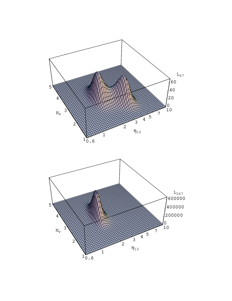
Figure 1: Likelihood functions $L_{47}$ (top) and $L_{247}$ (bottom) using $\hbox{$Y_{\rm p}$}=0.234\pm 0.0054$.

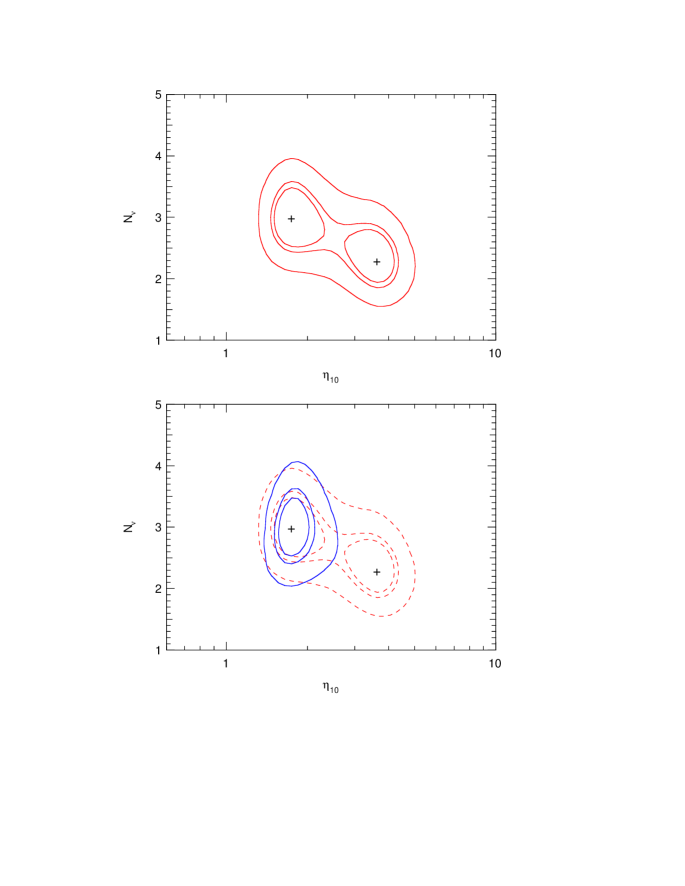
Figure 2: The top panel shows contours in the likelihood function $L_{47}$ for $\hbox{$Y_{\rm p}$}=0.234\pm 0.0054$. The contours represent 50% (innermost), 68% and 95% (outermost) confidence levels. The crosses mark the points of maximum likelihood. The bottom panel shows the equivalent results for $L_{247}$ (with $L_{47}$ shown dashed, for comparison.)

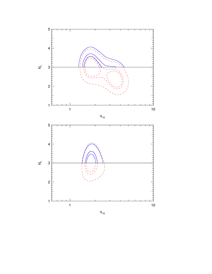
Figure 3: The top panel shows the likelihood function $L_{47}$ given the constraint $N_{\nu}\geq 3$. The contours represent 50%, 68% and 95% confidence levels. The unconstrained likelihood is shown dashed. In both cases $\hbox{$Y_{\rm p}$}=0.234\pm 0.0054$. The bottom panel shows the equivalent results for $L_{247}$.

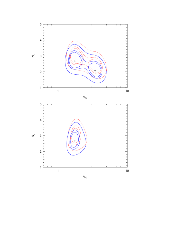
Figure 4: The top panel shows likelihood contours for $L_{47}$, with $\hbox{$Y_{\rm p}$}=0.230\pm 0.0058$. The contours represent 50%, 68% and 95% confidence levels. Results for $\hbox{$Y_{\rm p}$}=0.234\pm 0.0045$ are shown dashed for comparison. The bottom panel shows the equivalent results for $L_{247}$.

References

- [1] L.M. Krauss and P. Romanelli, ApJ, 358 (1990) 47.
- [2] M. Smith, L. Kawano, and R.A. Malaney, Ap.J. Supp., 85 (1993) 219.
- [3] P.J. Kernan and L.M. Krauss, Phys. Rev. Lett. 72 (1994) 3309.
- [4] L.M. Krauss and P.J. Kernan, Phys. Lett. B347 (1995) 347.
- [5] N. Hata, R.J. Scherrer, G. Steigman, D. Thomas, and T.P. Walker, Ap.J., 458 (1996) 637.
- [6] N. Hata, R. J. Scherrer, G. Steigman, D. Thomas, T. P. Walker, S. Bludman and P. Langacker, Phys. Rev. Lett. 75 (1995) 3977.
- [7] B.D. Fields, and K.A. Olive, Phys. Lett. B368 (1996) 103.
- [8] B.D. Fields, K. Kainulainen, K.A. Olive, and D. Thomas, astro-ph/9603009, New Astr., 1 (1996) 77.
- [9] J. Yang, M.S. Turner, G. Steigman, D.N. Schramm, and K.A. Olive, Ap.J. 281 (1984) 493.
- [10] G. Steigman, D.N. Schramm, and J. Gunn, Phys. Lett. B66 (1977) 202.
- [11] K.A. Olive, D.N. Schramm, G. Steigman, M.S. Turner, and J. Yang, Ap.J. 246 (1981) 557.
- [12] D. Black, Nature Physical Sci., 24 (1971) 148.
- [13] G. Steigman and M. Tosi, Ap.J. 401 (1992) 15; G. Steigman and M. Tosi, Ap.J. 453 (1995) 173.
- [14] C.J. Copi, D.N. Schramm, and M.S. Turner, Ap.J. 455 (1995) L95.
- [15] E. Vangioni-Flam, K.A. Olive, and N. Prantzos, Ap.J. 427 (1994) 618.
- [16] I. Iben, and J.W. Truran, Ap.J. 220 (1978) 980.
- [17] R.T. Rood, T.M. Bania, and T.L. Wilson, Nature 355 (1992) 618; R.T. Rood, T.M. Bania, T.L. Wilson, and D.S. Balser, 1995, in the Light Element Abundances, Proceedings of the ESO/EIPC Workshop, ed. P. Crane, (Berlin:Springer), p. 201.
- [18] K.A. Olive, R.T. Rood, D.N. Schramm, J.W. Truran, and E. Vangioni-Flam, Ap.J. 444 (1995) 680; D. Galli, F. Palla, F. Ferrini, and U. Penco, Ap.J. 443 (1995) 536; D. Dearborn, G. Steigman, and M. Tosi, Ap.J. 465 (1996) in press; S.T. Scully, M. Cassé, K.A. Olive, D.N. Schramm, J. Truran, and E. Vangioni-Flam, Ap.J. 462 (1996) 960.
- [19] T.P. Walker, G. Steigman, D.N. Schramm, K.A. Olive and K. Kang, Ap.J. 376 (1991) 51.
- [20] K.A. Olive and G. Steigman, Ap.J. Supp. 97 (1995) 49.
- [21] K.A. Olive and G. Steigman, Phys. Lett. B354 (1995) 357.
- [22] R.F. Carswell, M. Rauch, R.J. Weymann, A.J. Cooke, and J.K. Webb, MNRAS 268 (1994) L1; A. Songaila, L.L. Cowie, C. Hogan, and M. Rugers, Nature 368 (1994) 599.
- [23] S. Scully, M. Cassé, K.A. Olive, E. Vangioni-Flam, astro-ph/9607106, Ap. J. (1996) in press.
- [24] B.E.J. Pagel, E.A. Simonson, R.J. Terlevich and M. Edmunds, MNRAS 255 (1992) 325.
- [25] E. Skillman et al., Ap.J. Lett. (in preparation) 1996.
- [26] Y.I. Izatov, T.X. Thuan, and V.A. Lipovetsky, Ap.J. 435 435 (1994) 647.
- [27] K.A. Olive, and S.T. Scully, IJMPA 11 (1996) 409.
- [28] K.A. Olive, E. Skillman, and G. Steigman, in preparation
- [29] F. Spite, and M. Spite, A.A. 115 (1982) 357.
- [30] P. Molaro, F. Primas, and P. Bonifacio, A.A. 295 (1995) L47.
- [31] G. Steigman, B. Fields, K.A. Olive, D.N. Schramm, and T.P. Walker, Ap.J. 415 (1993) L35; M. Lemoine, D.N. Schramm, J.W. Truran, and C.J. Copi, Ap.J. (in press).
- [32] T.P. Walker, G. Steigman, D.N. Schramm, K.A. Olive and B. Fields, Ap.J. 413 (1993) 562; B.D. Fields, K.A. Olive, and D.N. Schramm, Ap.J. 435 (1994) 185; E. Vangioni-Flam, M. Cassé, B.D. Fields, and K.A. Olive, Ap.J. 468 (1996) 199.
- [33] M. Rugers and C.J. Hogan, Ap.J. 459 (1996) L1.
- [34] M. Rugers and C.J. Hogan, A.J. 111 (1996) 2135; R.F. Carswell, et al. MNRAS 278 (1996) 518; E.J. Wampler, et al. astro-ph/9512084, A.A. (1996) in press.
- [35] D. Tytler, X.-M. Fan, and S. Burles, Nature 381 (1996) 207; S. Burles and D. Tytler, Ap.J. 460 (1996) 584.
- [36] C.J. Copi, D.N. Schramm, and M.S. Turner, astro-ph/9606059.
- [37] N. Hata, G. Steigman, S. Bludman and P. Langacker, astro-ph/9603087.
- [38] K.A. Olive, astro-ph/96009071.