RHIC Detector Note

January 1996

Abstract

Coulomb-nuclear interference in the single transverse spin asymmetry $A_{N}$ is often considered as a possible absolute polarimeter for proton beams. The main uncertainty in this is the unknown hadronic spin-flip amplitude. This uncertainty is analyzed here in the context of the challenge of a $5\%$ polarization measurement at RHIC. Possible constraints on the spin-flip amplitude from measurements of the differential cross-section and the double transverse spin asymmetry $A_{NN}$ are discussed.

The addition of polarized proton beams to the RHIC facility presents the opportunity for an important new and unique physics program. In order to carry through this program, it is necessary to have a measurement of the beam polarization. How precise this measurement must be is not certain, but the challenge of a $5\%$ measurement has been made. A number of possibilities to do this are under discussion. A very attractive possibility is to make use of the Coulomb-nuclear interference (CNI) in the single transverse spin asymmetry $A_{N}$, which is enhanced in the small $t$ region : $|t|\sim 10^{-3}GeV^{2}$ [1, 2]. This method relies on the assumption that the hadronic amplitude is spin-independent for small $t$. In that case, the asymmetry is due solely to the interference between the electromagnetic spin-flip amplitude and the hadronic non-flip amplitude, which is determined by the proton-proton total cross-section. Hence $A_{N}$ can be calculated and the measurement of the left-right asymmetry with transversely polarized protons, which is equal to $PA_{N}$, would be an absolute measurement of the beam polarization $P$. The precision of the knowledge of $P$ would be determined by the precision of the asymmetry measurement and the accuracy of the calculation of $A_{N}$.

Unfortunately, there is very little known about the hadronic spin-flip amplitude in this small $t$ region—indeed, such a measurement is one of the goals of the RHIC program [3]. Experimentally, there is a fairly recent measurement at $200GeV/c$ from Fermilab, but it is not nearly precise enough to meet the challenge here, and the energy dependence is also unknown [4, 5]. Theoretically, so far as I know, there is no reliable means of calculating to the necessary accuracy the spin dependent amplitudes for small $t$. There is an extensive Regge pole fit to low energy data, at $6GeV/c$ and $12GeV/c$ lab momenta and for $t$ outside the CNI region [6]; it indicates a rather small hadronic spin flip amplitude, but it is large enough that one would have to correct for it to obtain a 5% measurement of $P$. In order to use CNI as a tool for measuring $P$ it is vital that one have a determination of the spin flip amplitude to the required precision that one can confidently use in the RHIC energy region. Therefore, in order to reach some conclusions about the demands of this method, I have adopted a natural and simple parametrization which has been used before, for example in a proposal to accelerate polarized protons at Fermilab [7]. We will see that, in spite of the enhancement of the CNI, one must know the hadronic spin-flip quite well, roughly to the precision required for $P$. We will see also that it is difficult to obtain this information independently from the measurement of the differential cross-section or from the double transverse spin asymmetry $A_{NN}$.

For completeness and the convenience of the reader, we will summarize here the basic formulae required. These are taken from the comprehensive paper by Buttimore, Gotsman, and Leader [2]. For proton-proton scattering, there are five independent amplitudes which will be specified here in terms of the helicities of the initial and final protons. Conventionally, these are identified in the following way:

$$\Phi_{1}(s,t) = \langle++|M|++\rangle$$ (1)

$$\Phi_{2}(s,t) = \langle++|M|--\rangle$$ (2)

$$\Phi_{3}(s,t) = \langle+-|M|+-\rangle$$ (3)

$$\Phi_{4}(s,t) = \langle+-|M|-+\rangle$$ (4)

$$\Phi_{5}(s,t) = \langle++|M|+-\rangle.$$ (5)

We will decompose each of these amplitudes $\Phi_{i}$ into a part called $f_{i}$ due to single photon exchange and a part called $h_{i}$ due to hadronic interactions. The $f_{i}$ are well known and given by

$$f_{1}(s,t)=f_{3}(s,t)=\frac{\alpha s}{t}g_{D}(t)^{2}$$ (6)

$$f_{2}(s,t)=-f_{4}(s,t)=\frac{\alpha s}{4m^{2}}(\mu-1)^{2}g_{D}(t)^{2}$$ (7)

$$f_{5}(s,t)=-\frac{\alpha s}{2m\sqrt{-t}}(\mu-1)g_{D}(t)^{2},\;\mbox{and}$$ (8)

$$g_{D}(t)=\frac{1}{(1-t/.71)^{2}},$$ (9)

to order $\alpha$. We have systematically neglected the proton mass $m$ with respect to $\sqrt{s}$, the center-of-mass energy and we have neglected the momentum transfer $\sqrt{-t}$ with respect to $m$. $g_{D}(t)$ is the dipole form factor of the proton and $\mu-1=1.79$. The fact that $f_{5}$ is less singular than $f_{1}$ or $f_{3}$ by a factor $\sqrt{-t}$ is a kinematic effect resulting from from angular momentum conservation: when $t\rightarrow 0$ the angular momentum is carried solely by the protons’ helicities. It is for the same reason that $f_{4}$ has a relative factor of $t$. These are absolute truths and will be properties of the full amplitudes $\Phi_{i}$. The remaining equalities are in a sense accidental and need not be shared with the amplitudes $h_{i}$. In practice, lacking any better knowledge, one often assumes $h_{1}(s,t)=h_{3}(s,t)$ and the other $h_{i}$ to be zero. For example, in the determination of the total cross-section from the differential cross-section and the optical theorem this is normally done, although it may not be correct.

The issue before us here is not very sensitive to any of these assumptions except that regarding $h_{5}$ and to that it is very sensitive.To see this, let us write down the expressions for the measurables in the same approximations as above. First the total cross-section is given by

$$\sigma_{tot}=\frac{4\pi}{s}Im(\Phi_{1}(s,t)+\Phi_{3}(s,t))|_{t=0};$$ (10)

note that this is not effected by the singularity of $f_{1}$ at $t=0$. Second, the differential cross-section is given by

$$\frac{d\sigma}{dt}=\frac{2\pi}{s^{2}}(|\Phi_{1}|^{2}+|\Phi_{2}|^{2}+|\Phi_{3}|^{2}+|\Phi_{4}|^{2}+4|\Phi_{5}|^{2}).$$ (11)

The single and double transverse spin asymmetries are given by

$$A_{N}\frac{d\sigma}{dt}=-\frac{4\pi}{s^{2}}Im\{\Phi_{5}^{*}(\Phi_{1}+\Phi_{2}+\Phi_{3}-\Phi_{4})\},$$ (12)

and

$$A_{NN}\frac{d\sigma}{dt}=\frac{4\pi}{s^{2}}\{2|\Phi_{5}|^{2}+Re(\Phi_{1}^{*}\Phi_{2}-\Phi_{3}^{*}\Phi_{4})\}.$$ (13)

Strictly speaking $A_{NN}$ is quite sensitive to all of the $\Phi_{i}$, but for the point that we wish to make the assumptions that $h_{1}=h_{3}$ and that $h_{2}=-h_{4}=0$ will not be important and we will adopt these conventional assumptions in order to focus on $h_{5}$.

In order to have a reasonable parametrization of the sensitivity, lacking any better knowledge, we will assume [7]

$$h_{5}(s,t)=\tau\,\sqrt{-t/m^{2}}\,h_{1}(s,t),$$ (14)

and, for small $t$, we assume the form

$$h_{1}(s,t)=s\,\frac{(\rho+i)}{8\pi}\,\sigma_{tot}\,e^{bt/2}.$$ (15)

We use values estimated to be appropriate for RHIC energy [8]: $b=15GeV^{-2},\\ \sigma_{tot}=62mb\;\mbox{and}\;\rho=0.13$. This parametrization is consistent with everything we know and so it represents a possible spin-flip amplitude. It does not seem to be a very strong assumption, provided we confine it to a small range of $t$. Note that $\tau$ is, in general, complex (and a function of $s$). With these forms $A_{N}$ has no explicit $s$-dependence, but there is significant $s$-dependence coming from the $s$-dependence of $\sigma_{tot}$ and $\rho$. In particular, the height of the peak in $A_{N}$ decreases with energy, roughly as $1/\sqrt{\sigma_{tot}}$ and the $t$-value of the peak moves toward zero, as $1/\sigma_{tot}$.

Because of this form the interference between $h_{5}$ and $f_{1}$ has the same shape in $A_{N}$ as the CNI interference between $h_{1}$ and $f_{5}$ so they just combine linearly, in the present approximation. If $\tau$ is real, then $h_{1}$ and $h_{5}$ are in phase and there is no purely hadronic spin-flip; the shape of $A_{N}(t)$ is thus very sensitive to $Im\tau$ as $t$ increases beyond the CNI region. Explicitly,

$$A_{N}\frac{d\sigma}{dt}=\frac{\alpha\sigma_{tot}e^{bt/2}}{2m\sqrt{-t}}\{(\mu-1)-2Re(\tau)-2\rho Im(\tau)\}+2Im(\tau)\frac{\sqrt{-t}}{m}\left(\frac{d\sigma}{dt}\right)_{hadronic}$$ (16)

Figure 1: $A_{N}$ for $\tau=0\;\mbox{solid curve},\tau=-0.1\;\mbox{dotted},\tau=+0.1\;\mbox{dashed}$

The main point of this exercise is made by Fig.1. Here we have plotted $A_{N}$ for three real values of $\tau$: $\tau=0$, which is the pure CNI case, and for comparison curves for $\tau=\pm 0.1$ This doesn’t seem like an unreasonably small value of $\tau$ and in assessing the usefulness of this method, it must be considered in the absence of other constraints. It is apparent from Fig.1 that all three curves have very similar shape and so, if for example one assumed that the solid curve were correct when in fact the dotted curve is correct, one would overestimate $P$ by about $10\%$. Because the shapes are the same over the entire $t$-range there is no way to separate $P$ and $A_{N}$ in the asymmetry measurement. To emphasize this, in Fig.2 we plot the ratios of the two curves with non-zero $\tau$ to the pure CNI curve over this $t$-range.

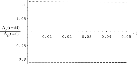
Figure 2: The ratio of $A_{N}$ for $\tau\pm 0.1$ to the pure CNI case, $\tau=0$

We see that these ratios are constant to a very high degree of accuracy.

If $\tau$ has a non-zero imaginary part, even a very small one can cause a significant modification of the shape of the $t$-dependence of $A_{N}$, because this leads to a purely hadronic contribution which grows, in this parametrization with $|t|$. One might hope to use this shape to get a handle on the size of $h_{5}$. However the real and imaginary parts are independent and so one cannot really make use of this. This is illustrated in Fig. 3 and Fig.4, in which $\tau$ is taken to have small positive and negative imaginary parts, respectively. The three curves in each case correspond to the same values for $Re\tau$ as in Fig.1; the imaginary parts are nearly the same for each of the curves in each figure, slightly adjusted to keep the ratios (as in Fig.2) nearly constant over the whole $t$-range. (This required fine-tuning for Fig.4 to ensure that the three curves cross 0 at the same value of $t$, but that is just cosmetic.) The point is that, although one can readily tell that there is deviation from pure CNI present, because the curves are in constant ratio one cannot separate $P$ from $A_{N}$ in these cases either.

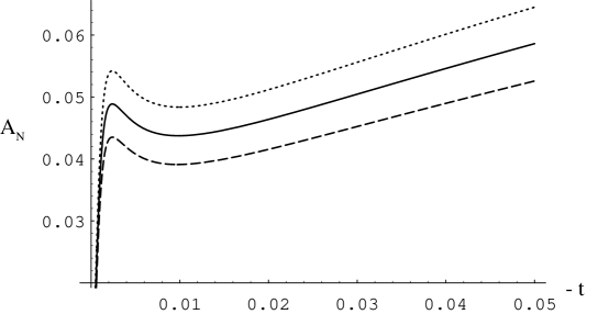
Figure 3: $A_{N}$ for $\tau=0.1i\;\mbox{solid curve},\tau=-0.1+0.11i\;\mbox{dotted},\tau=+0.1+0.09i\;\mbox{dashed}$

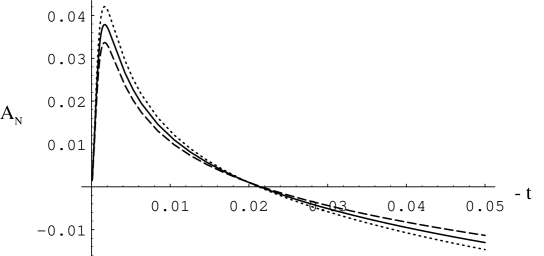
Figure 4: $A_{N}$ for $\tau=-0.05i\;\mbox{solid curve},\tau=-0.1-0.055i\;\mbox{dotted},\tau=+0.1-0.045i\;\mbox{dashed}$

It is important to see if there is additional information that could be made available that would constrain $h_{5}$ to be sufficiently small—or to measure it sufficiently well—to enable a $5\%$ measurement of $P$ to be made. In particular, $h_{5}$ enters into both the differential cross-section and the double transverse spin asymmetry $A_{NN}$ independently from the way it enters $A_{N}$: one enters an unpolarized process and the other enters a process for which the asymmetry is quadratic in $P$. In principle, this should be possible. The problem is that in neither one of these is the contribution of $h_{5}$ enhanced by interference with the one photon exchange as it is in $A_{N}$.

Consider first the differential cross-section. Buttimore [9] has derived a formula which gives a bound on $h_{5}$ in terms the differential cross-section, the total cross-section (presumably measured in an independent experiment) and the diffraction slope $b$. In the notation of our ansatz the bound reads

$$|\tau|<\sqrt{\frac{bm^{2}}{2}\left(\frac{16\pi b\sigma_{el}}{(1+\rho^{2})\sigma_{tot}^{2}}-1\right)}$$ (17)

The difficulty in using this is that $bm^{2}\sim 13$ and so even a bound of 0.1 on $\tau$ would require measuring the combination of quantities in parenthesis to be equal to 1 to better than one part in $10^{3}$. This bound does not seem to provide what is needed.

Finally, let us look at $A_{NN}$. It is useful to look at an approximate form for it to compare with Eq.(16). Using the same approximations with our ansatz we have

$$A_{NN}\frac{d\sigma}{dt}=\sigma_{tot}e^{bt/2}\frac{\alpha}{4m^{2}}(\mu-1)\{(\mu-1)\rho-4(\rho Re\tau-Im\tau)\}-2\frac{t}{m^{2}}|\tau|^{2}\left(\frac{d\sigma}{dt}\right)_{hadronic}$$ (18)

Notice that there is no purely one photon exchange contribution to this asymmetry either, although at first sight from Eq.13 it might look like there is. On the other hand the omitted terms containing $\Phi_{2}$ and $\Phi_{4}$ could make significant contributions; their presence would only make using this asymmetry a more problematic way of constraining $h_{5}$—we cannot do better than this. The important point is that the first term in not enhanced by a $1/\sqrt{-t}$ factor as is the corresponding term in Eq.(16). The second term is also suppressed by a similar factor. Thus, one is not surprised when one looks at Fig.5 and sees that $A_{NN}$ corresponding to the parameters in Fig.1, which translated into a $\pm 11\%$ variation in $P$, is only of order $0.1\%$. The corresponding values for the cases of Fig.3 and 4 are only about a factor of 2 larger than this. This, too, seems like a bound that is unlikely to be useful.

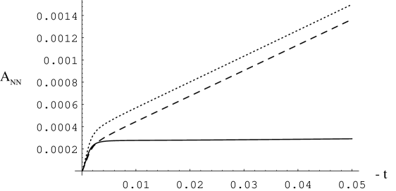
Figure 5: $A_{NN}$ for $\tau=0\;\mbox{solid curve},\tau=-0.1\;\mbox{dotted},\tau=+0.1\;\mbox{dashed}$

In conclusion, it is clear from these test cases that the uncertainty in $h_{5}$ must be at least as small as the precision required for $P$ in order for the CNI method to meet the requirement. Neither the $t$- dependence of $A_{N}$ nor the measurement of $\frac{d\sigma}{dt}$ or of $A_{NN}$ are likely to provide the information needed. Eventually through a combination of experiments and theory, we will likely know enough about the spin dependence of the proton-proton amplitudes to use CNI as an absolute polarimeter; in the meantime CNI might be used as an indication of the beam polarization but the measurements must be recognized as provisional and a source of systematic error. This underlines the importance of measuring the spin dependence of proton-proton scattering at RHIC.

I would like to thank Y. Makdisi, G. Bunce, J. Soffer, A. Krisch and E. Berger for valuable discussions.

References

- [1] B.Z.Kopeliovich and L.I.Lapidus,Sov.J.Nucl.Phys.19,114 (1974).
- [2] N.H.Buttimore, E.Gotsman and E.Leader, Phys.Rev.D 18, 694 (1978).
- [3] W. Guryn et al, RHIC proposal ”Experiment to Measure Total and Elastic pp Cross Sections at RHIC”, (1994).
- [4] N.Akchurin et al, Phys.Rev.D 48, 3026 (1993).
- [5] N.Akchurin, N.H.Buttimore and A.Penzo, Phys.Rev.D 51, 3944 (1995).
- [6] E.L.Berger, A.C.Irving and C.Sorenson, Phys.Rev.17, 2971 (1978).
- [7] SPIN Collaboration, Fermilab proposal ”Acceleration of Polarized Protons to 120 GeV and 1 TeV at Fermilab”, (1995).
- [8] M.Block, Proc. of International Conference on Elastic and Diffractive Scattering, ed. H.M.Fried,K.Kang and C.I.Tan, World Scientific (1994).
- [9] private communication from N.H.Buttimore via A. Penzo (1995).