Color-Octet Contributions in
the Associate $J/\psi+\gamma$ Hadroproduction

Abstract

Color-octet contributions to the associate $J/\psi+\gamma$ hadroproduction are studied in detail, and found to be negligible, compared to the ordinary color-singlet contribution. Within the color-singlet model the $J/\psi+\gamma$ production in the leading order is possible only through gluon-gluon fusion process. Therefore, the associate $J/\psi+\gamma$ hadroproduction remains to be useful as a clean channel to probe the gluon distribution inside proton, to study heavy quarkonia production mechanism, and to find proton’s spin structure.

I Introduction

Up to very recently the conventional color-singlet model [1, 2] had been used as only possible mechanism to describe the production and decay of the heavy quarkonium such as $J/\psi$ and $\Upsilon$. An artificial $K$-factor ($\sim$ 2–5) was first introduced to compensate the gap between the theoretical prediction and experimental data. The uncertainties related to this large $K$-factor are the following: We don’t know precisely the correct normalization of the bound state wave function, the possible next-to-leading order contributions, the mass of the heavy quark inside the bound state, etc. However, even with this large $K$-factor some experimental data are found to be difficult to describe. For the direct $J/\psi$ production with large $p_{{}_{T}}$ in $p\overline{p}$ collisions, the dominant mechanism has been found to be through final parton fragmentation [3]. As applications of this fragmentation mechanism, various studies of prompt charmonium production at the Tevatron collider [4, 5, 6] have been carried out, and the CDF data on the prompt $J/\psi$ production [7] qualitatively meet these theoretical predictions. Nevertheless, the $\psi^{\prime}$ production rate at CDF is about 30 times larger than the theoretical predictions, which is the so-called $\psi^{\prime}$ anomaly, even after considering the fragmentation mechanisms of $g\rightarrow\psi^{\prime}$ and $c\rightarrow\psi^{\prime}$. As a scenario to resolve this $\psi^{\prime}$ anomaly, the color-octet production mechanism was proposed [8]. By using this idea, heavy quarkonium (charmonium) hadroproduction through the color-octet $(c\overline{c})_{8}$ pair in various partial wave states $(^{2S+1}L_{J})$ has been studied in addition to the color-octet gluon fragmentation approach [9, 10]. We note that the inclusive $\Upsilon$ production at the Tevatron also shows an excess of the data over theoretical estimates based on perturbative QCD and the color-singlet model [11]. In this case, the $p_{{}_{T}}$ of the $\Upsilon$ is not so high, so that the gluon fragmentation picture may not be a good approximation any more.

Since it has been proposed that the color-octet mechanism can resolve the $\psi^{{}^{\prime}}$ anomaly at the Tevatron collider, it is quite important to test this mechanism at other high energy heavy quarkonium production processes. Up to now, the following processes have been theoretically considered: inclusive $J/\psi$ production at the Tevatron collider and at fixed target experiments [9, 10, 12], spin alignment of leptons to the decayed $J/\psi$ [13], the polar angle distribution of the $J/\psi$ in $e^{+}e^{-}\to J/\psi+X$ [14], inclusive $J/\psi$ productions in $B$ meson decays [15, 16] and in $Z^{0}$ decays at LEP [17, 18, 19], $J/\psi$ photoproduction [16, 20, 21, 22], and color-octet $J/\psi$ production in $\Upsilon$ decays [23]. For more details on recent progress, see Ref. [24], which summarizes the theoretical developments on the quarkonium production. Recently, the helicity decomposition method in NRQCD factorization formalism was developed by Braaten and Chen [25]. With this method, polarized $J/\psi$ production in $B$ decay was considered in Ref. [26]. In Ref. [25, 27], it was pointed out that there are interference terms of different ${}^{3}P_{J}$ contributions in polarized $J/\psi$ production.

In this work, we investigate the color-octet mechanism for associate $J/\psi+\gamma$ production in hadronic collisions. The associate $J/\psi+\gamma$ production has been first proposed as a clean channel to probe the gluon distribution inside the proton or photon [28], and then to study the heavy quarkonia production mechanism [29] as well as to investigate the proton’s spin structure [30]. If the color-octet mechanism gives a significant contribution to this process, the merit of this process to probe the gluon distribution etc. would be decreased or one should find suitable cuts to get rid of this new contribution. Associate $J/\psi+\gamma$ production has also been studied as a significant QCD background to the decay of heavier $P$-wave charmonia ($\chi_{cJ}(P)$) in fixed target experiments [31, 32] within the color-singlet model [33]. In Ref. [34], the fragmentation contribution from $p+\bar{p}\rightarrow(c~{}{\rm or}~{}g)+\gamma+X\rightarrow J/\psi+\gamma+X$ at Tevatron energies ($\sqrt{s}$=1.8 TeV) is studied, and these fragmentation channels are found to be significantly suppressed compared to the conventional color-singlet gluon-gluon fusion process.

In Section 2, we explain in detail the method to deal with inclusive heavy quarkonium production, following the nonrelativistic-QCD (NRQCD) factorization formalism given by Bodwin, Braaten and Lepage (BBL) [35]. A summary of the kinematics related to the $p_{{}_{T}}$ and $M_{J/\psi+\gamma}$ distributions is also given in this Section. In Section 3, we discuss in detail the $p_{{}_{T}}$ and $M_{J/\psi+\gamma}$ distributions in the hadronic $J/\psi+\gamma$ production, and compare the color-octet contribution with the color-singlet gluon-gluon fusion contribution. Section 3 also contains our conclusions.

II Hadroproduction of $J/\psi+\gamma$

A General Discussions

Now we consider the associate production of a $J/\psi$ and a photon at hadronic colliders and fixed target experiments, including the new contribution from the color-octet mechanism in addition to the usual color-singlet contribution. The only possible subprocess in the framework of the color-singlet model in the leading order is through gluon-gluon fusion,

$$g+g\rightarrow\gamma+(c\overline{c})(^{3}S^{(1)}_{1})(\rightarrow J/\psi).~{}~{}~{}~{}~{}({\rm See~{}Fig.~{}\ref{fig:fusion}})$$ (1)

This gluon-gluon fusion process for the associate $J/\psi+\gamma$ production is again possible within the color-octet mechanism. (See Fig. 1). However, in the leading order color-octet contributions there also exist many more subprocesses, which are

$$g+g \rightarrow \gamma+(c\overline{c})(^{1}S^{(8)}_{0})(\rightarrow J/\psi),$$ (2)

$$g+g \rightarrow \gamma+(c\overline{c})(^{3}P^{(8)}_{J})(\rightarrow J/\psi),$$ (3)

$$q+\overline{q} \rightarrow \gamma+(c\overline{c})(^{1}S^{(8)}_{0})(\rightarrow J/\psi),$$ (4)

$$q+\overline{q} \rightarrow \gamma+(c\overline{c})(^{3}P^{(8)}_{J})(\rightarrow J/\psi),$$ (5)

$$q+\overline{q} \rightarrow \gamma+(c\overline{c})(^{3}S^{(8)}_{1})(\rightarrow J/\psi).$$ (6)

These subprocesses are possible through the effective vertices of

$$\gamma+g\rightarrow(c\overline{c})(^{1}S_{0}^{(8)}~{}~{}{\rm or}~{}~{}^{3}P_{J}^{(8)}),$$ (7)

which is shown in Fig. 2, and

$$q+\overline{q}\rightarrow(c\overline{c})(^{3}S_{1}^{(8)}),$$ (8)

which is shown in Fig. 3. We note that the $(^{3}S_{1}^{(8)})$ channel in Eq. (7) is vanishing, even though the gluon is not on its mass shell. The Feynman diagram for the gluon initiated subprocesses, Eqs. (2, 3), is shown in Fig. 4 (a). For the case of quark initiated subprocesses, there are two kinds of diagrams; The Feynman diagram for quark initiated subprocesses Eqs. (4, 5), due to the effective vertex Eq. (7), is shown in Fig. 4 (b). The other diagrams, which are possible through the effective vertex, Eq. (8), are shown in Fig. 5.

We first perform a naive power counting analysis of those various subprocesses. Free particle amplitude-squared for the color-singlet gluon-gluon fusion process (1) is $[{\cal O}(\alpha\alpha_{s}^{2})]$. In the NRQCD framework [35], the color-octet ($Q\overline{Q}$) states can also form a physical $J/\psi$ state with dynamical gluons inside the quarkonium with wavelengths much larger than the characteristic size of the bound state ($\sim$$1/(M_{Q}v_{Q})$). In Coulomb gauge, which is a natural gauge for analyzing heavy quarkonium, these dynamical gluons enter into the Fock state decomposition of physical state of $J/\psi$ as

$$|J/\psi\rangle= {\cal O}(1)|(Q\overline{Q})(^{3}S_{1}^{(1)})\rangle+{\cal O}(v_{Q})|(Q\overline{Q})(^{3}P_{J}^{(8)})g\rangle$$ (9)

$$+ {\cal O}(v_{Q}^{2})|(Q\overline{Q})(^{3}S_{1}^{(1,8)})gg\rangle+{\cal O}(v_{Q}^{2})|(Q\overline{Q})(^{1}S_{0}^{(8)})g\rangle+...~{}.$$ (10)

In general, a state $(Q\overline{Q})(^{2S+1}L_{J})$ can make a transition to $(Q\overline{Q})(^{2S+1}(L\pm 1)_{J})$, or more specifically $(Q\overline{Q})(^{3}P_{J}^{(8)})\rightarrow(Q\overline{Q})(^{3}S_{1}^{(1)})$ through the emission of a soft gluon (chromo-electric dipole transition), and it is an order of $v_{Q}$ suppressed compared to the color-singlet hadronization. For the case of chromo-magnetic dipole transition, such as $(Q\overline{Q})(^{1}S_{0}^{(8)})\rightarrow(Q\overline{Q})(^{3}S_{1}^{(1)})$, it is suppressed by $v_{Q}$ at the amplitude level. If we also consider the fact that the $P$ wave state is $M_{Q}v_{Q}$ order higher than $S$ wave state in the amplitude level, one can naively estimate that the transitions

$$(Q\overline{Q})(^{3}P_{J}^{(8)})\rightarrow J/\psi+X~{}~{}~{}{\rm and}~{}~{}~{}(Q\overline{Q})(^{1}S_{0}^{(8)})\rightarrow J/\psi+X$$ (11)

are commonly $v_{Q}^{4}$ order suppressed at the amplitude-squared level, compared to the transition

$$(Q\overline{Q})(^{3}S_{1}^{(1)})\rightarrow J/\psi~{}.$$ (12)

Since these color-octet processes have the same order ${\cal O}(\alpha\alpha_{s}^{2})$ as that of the color-singlet gluon-gluon fusion process in free particle scattering amplitude, the color-octet subprocesses are order $v_{Q}^{4}$ suppressed compared to the color-singlet gluon-gluon fusion subprocess.

However, such analyses are only naive power counting, and do not guarantee that the color-octet contributions are suppressed compared to the color-singlet gluon-gluon fusion contribution all over the allowed kinematical region. If we consider inclusive $J/\psi$ photoproduction via $2\rightarrow 2$ subprocesses, as shown in Refs. [16, 20], color-octet contributions dominate in some kinematical region, even if the naive power counting predicts the suppression of color-octet contributions compared to the color-singlet one. In this respect, it is worthwhile to investigate in detail how much the color-octet mechanism contributes to the $J/\psi+\gamma$ hadroproduction.

In order to predict numerically the physical production rate, we need to know a few nonperturbative parameters characterizing the fragmentation of the color-octet objects into the physical color-singlet $J/\psi$. These nonperturbative matrix elements for the color-octet operators have not been determined completely yet. After fitting the inclusive $J/\psi$ production at the Tevatron collider, using the usual color-singlet $J/\psi$ production, the cascades production from $\chi_{c}(1P)$, and the new color-octet contributions, the authors of Ref. [10] have determined

$$\langle 0|O_{8}^{\psi}(^{3}S_{1})|0\rangle = (6.6\pm 2.1)\times 10^{-3}~{}{\rm GeV}^{3},$$ (13)

$$\frac{\langle 0|{\cal O}_{8}^{\psi}({{}^{3}P_{0}})|0\rangle}{M_{c}^{2}}+\frac{\langle 0|{\cal O}_{8}^{\psi}({{}^{1}S_{0}})|0\rangle}{3} = (2.2\pm 0.5)\times 10^{-2}~{}{\rm GeV}^{3},$$ (14)

with $M_{c}=1.48$ GeV. Although the numerical values of two matrix elements, $\langle 0|{\cal O}_{8}^{\psi}(^{3}P_{0})|0\rangle$ and $\langle 0|{\cal O}_{8}^{\psi}(^{1}S_{0})|0\rangle$, are not separately known in Eq. (14), one can still extract some useful information from them. Assuming both of the color-octet matrix elements in Eq. (14) are positive definite, then one has[16]

$$0<\langle 0|{\cal O}_{8}^{\psi}({{}^{1}S_{0}})|0\rangle<(6.6\pm 1.5)\times 10^{-2}~{}{\rm GeV}^{3},$$ (15)

$$0<{\langle 0|{\cal O}_{8}^{\psi}({{}^{3}P_{0}})|0\rangle\over M_{c}^{2}}<(2.2\pm 0.5)\times 10^{-2}~{}{\rm GeV}^{3}.$$ (16)

These inequalities could provide us with a few predictions on various quantities related to inclusive $J/\psi$ productions in other processes, and also enable us to test the idea of color-octet mechanism in the associate $J/\psi+\gamma$ production process.

B Kinematics

Let us consider the process

$$a(p_{1})_{/p(P_{1})}+b(p_{2})_{/\overline{p}(P_{2})}\rightarrow J/\psi(P)+\gamma(k).$$ (17)

in $p\overline{p}$ (or alternatively $pp$) collisions. We can express the momenta of the incident hadrons $(p,~{}\bar{p})$ and partons $(a,~{}b)$ in the $p\overline{p}$ CM frame as

$$P_{1}=\frac{\sqrt{s}}{2}(1,+1,0),~{}~{} ~{}~{}p_{1}=\frac{\sqrt{s}}{2}(x_{1},+x_{1},0),$$ (18)

$$P_{2}=\frac{\sqrt{s}}{2}(1,-1,0),~{}~{} ~{}~{}p_{2}=\frac{\sqrt{s}}{2}(x_{2},-x_{2},0),$$ (19)

where the first component is the energy, the second is longitudinal momentum, and the third is the transverse component of the particle’s momentum. The variables $x_{1}$ and $x_{2}$ are the momentum fractions of the partons. The momenta of the outgoing particles are given by,

$$P=(E^{\psi},P_{L}^{\psi},+P_{T}) = (M_{T}\cosh y^{\psi},M_{T}\sinh y^{\psi},+P_{T}),$$ (20)

$$k~{}=(E^{\gamma},P_{L}^{\gamma},-P_{T}) = (~{}P_{T}\cosh y^{\gamma},~{}P_{T}\sinh y^{\gamma},-P_{T}),$$ (21)

where $P_{T}$ is the common transverse momentum of the outgoing particles, $M_{T}$ is the transverse mass of the outgoing $J/\psi$, and $y^{\psi}$ (or $y^{\gamma}$) is the rapidity of $J/\psi$ (or $\gamma$). Some useful relations among the above variables are:

$$E^{\psi}+P_{L}^{\psi}=M_{T}e^{+y^{\psi}},~{}~{} ~{}~{}E^{\psi}-P_{L}^{\psi}=M_{T}e^{-y^{\psi}},$$ (22)

$$E^{\gamma}+P_{L}^{\gamma}=~{}P_{T}e^{+y^{\gamma}},~{}~{} ~{}~{}E^{\gamma}-P_{L}^{\gamma}=~{}P_{T}e^{-y^{\gamma}}.$$ (23)

The Mandelstam variables are defined respectively as

$$s = (P_{1}+P_{2})^{2},$$ (24)

$$\hat{s}=(p_{1}+p_{2})^{2} = 2x_{1}x_{2}P_{1}\cdot P_{2}=x_{1}x_{2}s,$$ (25)

$$\hat{t}=(p_{1}-~{}k)^{2} = -x_{1}\sqrt{s}P_{T}e^{-y^{\gamma}}=(p_{2}-P)^{2}=M_{\psi}^{2}-x_{2}\sqrt{s}M_{T}e^{+y^{\psi}},$$ (26)

$$\hat{u}=(p_{2}-~{}k)^{2} = -x_{2}\sqrt{s}P_{T}e^{+y^{\gamma}}=(p_{1}-P)^{2}=M_{\psi}^{2}-x_{1}\sqrt{s}M_{T}e^{-y^{\psi}},$$ (27)

$$M_{\psi}^{2} = \hat{s}+\hat{t}+\hat{u}.$$ (28)

The last equation, representing the energy-momentum conservation, leads to

$$\sqrt{s}M_{T}(x_{2}e^{y^{\psi}}+x_{1}e^{-y^{\psi}}) = \hat{s}+M_{\psi}^{2},$$ (29)

$$\sqrt{s}P_{T}~{}(x_{2}e^{y^{\gamma}}+x_{1}e^{-y^{\gamma}}) = \hat{s}-M_{\psi}^{2}.$$ (30)

After introducing dimensionless variables,

$$x_{T}=2P_{T}/\sqrt{s},\hskip 19.91684pt\overline{x}_{T}=2M_{T}/\sqrt{s}\hskip 14.22636pt{\rm and}\hskip 14.22636pt\tau=M^{2}_{\psi}/s,$$ (31)

we can solve the energy momentum relation to get $x_{2}$ in terms of other variables as

$$x_{2}=\frac{x_{1}\overline{x}_{T}e^{-y^{\psi}}-2\tau}{2x_{1}-\overline{x}_{T}e^{+y^{\psi}}}\hskip 14.22636pt{\rm or}\hskip 14.22636ptx_{2}=\frac{x_{1}x_{T}e^{-y^{\gamma}}+2\tau}{2x_{1}-x_{T}e^{+y^{\gamma}}}.$$ (32)

We also obtain the relations for rapidities of the outgoing particles in terms of $x_{1}$, $x_{2}$, $x_{T}$, $\overline{x}_{T}$ and $\tau$ as following

$${\rm exp}({y^{\psi}}) = \frac{(x_{1}x_{2}+\tau)+\sqrt{(x_{1}x_{2}+\tau)^{2}-x_{1}x_{2}\overline{x}_{T}^{2}}}{x_{2}\overline{x}_{T}},$$ (33)

$${\rm exp}({y^{\gamma}}) = \frac{(x_{1}x_{2}-\tau)-\sqrt{(x_{1}x_{2}-\tau)^{2}-x_{1}x_{2}x_{T}^{2}}}{x_{2}x_{T}}.$$ (34)

In order to get the distributions in the invariant mass $M_{J/\psi+\gamma}(\equiv\sqrt{\hat{s}})$ and transverse momentum $P_{{}_{T}}$ for the process $g+g\rightarrow J/\psi+\gamma$ process, we express the differential cross section as

$$d\sigma = f_{g/p}(x_{1},Q^{2})f_{g/\overline{p}}(x_{2},Q^{2})\frac{d\hat{\sigma}}{d\hat{t}}dx_{1}dx_{2}d\hat{t}$$ (35)

$$= f_{g/p}(x_{1},Q^{2})f_{g/\overline{p}}(x_{2},Q^{2})\frac{d\hat{\sigma}}{d\hat{t}}J\left(\frac{x_{1}x_{2}\hat{t}}{x_{1}x_{T}M_{J/\psi+\gamma}}\right)dx_{1}dx_{T}dM_{J/\psi+\gamma}$$ (36)

$$= f_{g/p}(x_{1},Q^{2})f_{g/\overline{p}}(x_{2},Q^{2})\frac{d\hat{\sigma}}{d\hat{t}}J\left(\frac{x_{1}x_{2}\hat{t}}{x_{1}y^{\psi}P_{T}}\right)dx_{1}dy^{\psi}dP_{T},$$ (37)

where the corresponding Jacobians are given by

$$J\left(\frac{x_{1}x_{2}\hat{t}}{x_{1}x_{T}M_{J/\psi+\gamma}}\right)=\frac{2x_{2}x_{T}M_{J/\psi+\gamma}}{\overline{x}_{T}(x_{2}e^{+y_{\psi}}-x_{1}e^{-y_{\psi}})}~{}~{}~{}{\rm and}~{}~{}~{}J\left(\frac{x_{1}x_{2}\hat{t}}{x_{1}y^{\psi}P_{T}}\right)=\frac{4x_{1}x_{2}P_{T}}{2x_{1}-\overline{x}_{T}e^{+y^{\psi}}}$$ (38)

Then the distributions are expressed as

$$\frac{d\sigma}{dM_{J/\psi+\gamma}} = \int dx_{1}~{}dx_{T}J\left(\frac{x_{1}x_{2}\hat{t}}{x_{1}x_{T}M_{J/\psi+\gamma}}\right)\frac{d^{3}\hat{\sigma}}{dx_{1}dx_{2}d\hat{t}}~{},$$ (39)

$$\frac{d\sigma}{dP_{T}} = \int dx_{1}~{}dy^{\psi}J\left(\frac{x_{1}x_{2}\hat{t}}{x_{1}y^{\psi}P_{T}}\right)\frac{d^{3}\hat{\sigma}}{dx_{1}dx_{2}d\hat{t}}~{}.$$ (40)

And the allowed regions of the variables are given by

$$\frac{M_{J/\psi+\gamma}^{2}}{s}\leq x_{1}\leq 1,$$ (41)

$$\hat{s}=M_{J/\psi}^{2}=x_{1}x_{2}s\geq M_{J/\psi}^{2},$$ (42)

$$0\leq x_{T}\leq\frac{(x_{1}x_{2}-\tau)}{\sqrt{x_{1}x_{2}}}.$$ (43)

C The Nonrelativistic-QCD (NRQCD) Factorization Formalism

First we consider the general method to get the NRQCD cross section for the process $a+b\rightarrow(Q\overline{Q})(^{2S+1}L^{(1,8)}_{J})(\rightarrow H)+c$, where $H$ is the final state heavy quarkonium and $(Q\overline{Q})(^{2S+1}L^{(1,8)}_{J})$ is the intermediate $(Q\overline{Q})$ pair which has the corresponding spectroscopic state. From now on, we use the subscript $n$ to represent the spectroscopic $(Q\overline{Q})$ state of $(^{2S+1}L_{J}^{(n=1,8)})$, for simplicity. Once the on-shell scattering amplitude of the process ${\cal A}(a+b\rightarrow Q+\overline{Q}+c)$ is given, we can expand the amplitude in terms of relative momentum $q$ of the quarks inside the bound state because the quarks, which make up the bound state, are heavy. For more details of the method to deal with the heavy quarkonium production following the BBL formalism [35], we refer to Refs. [9, 10, 16]. The heavy quarkonium $H$ production cross section $a(p_{1})+b(p_{2})\rightarrow(Q\overline{Q})_{n}(P)+c(p_{3})\rightarrow H+c+X$ is given by

$$\frac{d\hat{\sigma}}{d\hat{t}} \left(a(p_{1})+b(p_{2})\rightarrow(Q\overline{Q})_{n}(P)+c(p_{3})\rightarrow H+c+X\right)$$ (45)

$$=\frac{1}{C_{n}M_{Q}}\times\frac{d\hat{\sigma}^{\prime}_{n}}{d\hat{t}}\times\frac{\langle 0|{\cal O}_{n}^{H}|0\rangle}{2J+1},$$

where

$$\frac{d\hat{\sigma}^{\prime}_{n}}{d\hat{t}}=\frac{1}{16\pi\hat{s}^{2}}\overline{\sum}|{\cal M}^{\prime}\left(a(p_{1})+b(p_{2})\rightarrow(Q\overline{Q})_{n}(P)+c(p_{3})\right)|^{2}.$$ (46)

Here, ${\cal M}^{\prime}$ is the amplitude of the process

$$a(p_{1})+b(P_{2})\rightarrow(Q\overline{Q})_{n}(P)+c(p_{3}),$$ (47)

which can be obtained by integrating the free particle amplitude over the relative momentum of the quark inside the intermediate state $(Q\overline{Q})_{n}(P)$, after projecting appropriate spectroscopic state Clebsch-Gordon coefficients. The parameter $C_{n}$ is defined by

$$C_{n}=\left\{\begin{array}[]{cl}2N_{c}&({\rm color-singlet}),\\ N_{c}^{2}-1&({\rm color-octet}).\end{array}\right.$$ (48)

And $\langle 0|{\cal O}_{n}^{H}|0\rangle$ is the non-perturbative matrix element representing the transition

$$(Q\overline{Q})(^{2S+1}L_{J}^{(1,8)})\to H.$$ (49)

Finally, $J$ denotes the angular momentum of the intermediate state $(Q\overline{Q})(^{2S+1}L_{J}^{(1,8)})$, not of the physical state $H$. For the case of color-singlet intermediate state, which has the same spectroscopic configuration with $H$, we can relate the matrix elements to the radial wave-function of the bound state as

$$\frac{\langle 0|{\cal O}_{n}^{H}|0\rangle}{C_{n}\times(2J+1)}=\left\{\begin{array}[]{l}\frac{1}{4\pi}|R_{S}(0)|^{2}~{}~{}~{}(S-{\rm wave}),\\ \\ \frac{3}{4\pi}|R_{P}^{\prime}(0)|^{2}~{}~{}~{}(P-{\rm wave}).\end{array}\right.$$ (50)

For example, if we consider the $\psi$ production via $(^{3}S_{1}^{(1)})$, $(^{1}S_{0}^{(8)})$, $(^{3}S_{1}^{(8)})$, $(^{3}P_{0}^{(8)})$, $(^{3}P_{1}^{(8)})$ and $(^{3}P_{2}^{(8)})$ intermediate states, then the partonic subprocess cross sections are given by

$$\frac{d\hat{\sigma}}{d\hat{t}}({\rm octet}) = \frac{1}{8M_{c}}\left(\frac{d\hat{\sigma}^{\prime}}{d\hat{t}}(^{1}S_{0}^{(8)})\times\langle 0|{\cal O}^{\psi}(^{1}S_{0}^{(8)})|0\rangle+\frac{\hat{d\sigma}^{\prime}}{d\hat{t}}(^{3}S_{1}^{(8)})\times\frac{\langle 0|{\cal O}^{\psi}(^{3}S_{1}^{(8)})|0\rangle}{3}\right.$$ (52)

$$\left.\hskip 56.9055pt+\langle 0|{\cal O}^{\psi}(^{3}P_{0}^{(8)})|0\rangle\times\sum_{J}\frac{d\hat{\sigma}^{\prime}}{d\hat{t}}(^{3}P_{J}^{(8)})\right),$$

$$\frac{d\hat{\sigma}}{d\hat{t}}({\rm singlet}) = \frac{1}{M_{c}}~{}\frac{|R_{S}(0)|^{2}}{4\pi}\frac{d\hat{\sigma}^{\prime}}{d\hat{t}}(^{3}S_{1}^{(1)}),$$ (53)

after imposing the heavy quark spin symmetry

$$\langle 0|{\cal O}^{J/\psi}(^{3}P_{J}^{(8)})|0\rangle=(2J+1)\langle 0|{\cal O}^{J/\psi}(^{3}P_{0}^{(8)})|0\rangle.$$ (54)

The subprocess cross section for the color-singlet gluon-gluon fusion [1] is well known:

$$\frac{d\hat{\sigma}}{d\hat{t}}({\rm singlet})=\frac{{\cal N}_{1}}{16\pi\hat{s}^{2}}~{}\left[\frac{\hat{s}^{2}(\hat{s}-4M_{c}^{2})^{2}+\hat{t}^{2}(\hat{t}-4M_{c}^{2})^{2}+\hat{u}^{2}(\hat{u}-4M_{c}^{2})^{2}}{(\hat{s}-4M_{c}^{2})^{2}(\hat{t}-4M_{c}^{2})^{2}(\hat{u}-4M_{c}^{2})^{2}}\right],$$ (55)

where the overall normalization ${\cal N}_{1}$ is defined as

$${\cal N}_{1}={4\over 9}~{}(4\pi\alpha_{s})^{2}(4\pi\alpha)e_{c}^{2}~{}M_{c}^{3}G_{1}(J/\psi).$$ (56)

The parameter $G_{1}(J/\psi)$, which is defined in NRQCD as

$$G_{1}(J/\psi)=\frac{\langle 0|{\cal O}(^{3}S_{1}^{(1)})|0\rangle}{3M_{c}^{2}}=\frac{3}{2\pi M_{c}^{2}}|R_{S}(0)|^{2},$$ (57)

is proportional to the probability of a color-singlet $(c\overline{c})$ pair in the $(^{3}S^{(1)}_{1})$ partial wave state to form a physical $J/\psi$ state. It is related to the leptonic decay width

$$\Gamma(J/\psi\rightarrow l^{+}l^{-})={2\over 3}~{}\pi e_{c}^{2}\alpha^{2}~{}G_{1}(J/\psi),$$ (58)

where $e_{c}=2/3$. From the measured leptonic decay rate of $J/\psi$, one can extract

$$G_{1}(J/\psi)\approx 106~{}~{}{\rm MeV}.$$ (59)

After including the radiative corrections of ${\cal O}(\alpha_{s})$ with $\alpha_{s}(M_{c})=0.27$, this value is increased to $\approx 184$ MeV. Relativistic corrections tend to increase $G_{1}(J/\psi)$ further to $\sim 195$ MeV [15].

For the case of color-octet subprocesses, we can use the average-squared amplitude of the processes $\gamma+g~{}({\rm or}~{}q)\rightarrow~{}(c\overline{c})(^{2S+1}L_{J}^{(8)})+g~{}({\rm or}~{}q)$ in Ref. [16], after crossing ($k\rightarrow-k$  and  $q_{2}\rightarrow-q_{2}$)

$$\overline{\sum}|{\cal M}^{\prime}|^{2}(g+g~{} \rightarrow~{}(c\overline{c})(^{2S+1}L_{J}^{(8)})+\gamma)(\hat{s},\hat{t},\hat{u})$$ (61)

$$=\frac{1}{8}|{\cal M}^{\prime}|^{2}(\gamma+g\rightarrow~{}(c\overline{c})(^{2S+1}L_{J}^{(8)})+g)(\hat{t},\hat{s},\hat{u}),$$

$$\overline{\sum}|{\cal M}^{\prime}|^{2}(q+\overline{q}~{} \rightarrow~{}(c\overline{c})(^{2S+1}L_{J}^{(8)})+\gamma)(\hat{s},\hat{t},\hat{u})$$ (63)

$$=\frac{1}{3}|{\cal M}^{\prime}|^{2}(\gamma+q\rightarrow~{}(c\overline{c})(^{2S+1}L_{J}^{(8)})+q)(\hat{t},\hat{s},\hat{u}).$$

As previously explained, there is only one color-singlet subprocess, but 9 color-octet subprocesses are contributing to the process

$$p+p~{}(\overline{p})\rightarrow J/\psi+\gamma+X.$$ (64)

Whereas the initial partons for the color-singlet process are only the gluons, quarks can also be the initial partons for the color-octet subprocesses. For the $(^{3}S_{1}^{(8)})$ channel, the gluon contribution corresponding to Fig. 4 (a) is absent because the effective vertex corresponding to Fig. 2 is vanishing. Using the parton level differential cross sections for various channels, in the next section we discuss in detail the $p_{{}_{T}}$ and $M_{J/\psi+\gamma}$ distributions in the hadronic $J/\psi+\gamma$ production. We also compare the color-octet contributions with the color-singlet gluon-gluon fusion contribution.

III Numerical Results and Conclusions

Now, we are ready to show the numerical results from the analytic expressions obtained in the previous section. The results are quite sensitive to the numerical values of QCD coupling constant $\alpha_{s}$, mass of charm quark $M_{c}$, and the factorization scale $Q$. For numerical predictions, we used $\alpha_{s}(M_{c}^{2})=0.27$, $M_{c}=1.48$ GeV and $Q^{2}=(M_{T}/2)^{2}$, where $M_{T}$ is the transverse mass of the outgoing $J/\psi$. For the structure functions, we have used the most recent ones, MRSA [36] and CTEQ3M [37], and it turns out that both sets of structure functions give more or less the same results within $\sim 10\%$.

We use the numerical value of the color-octet matrix element, shown in Eq. (2.12),

$$\langle 0|{\cal O}^{\psi}(^{3}S_{1}^{(8)})|0\rangle=(6.6\pm 2.1)\times 10^{-3}{\rm GeV}^{3}.$$ (65)

And since the matrix elements $\langle 0|{\cal O}_{8}^{\psi}({{}^{1}S_{0}})|0\rangle$ and $\langle 0|{\cal O}_{8}^{\psi}({{}^{3}P_{0}})|0\rangle$ are not determined separately, we present the two extreme values allowed by Eqs. (2,13,2.14,16) as

$${}^{1}S_{0}{\rm~{}~{}saturated~{}~{}case} : \langle 0|{\cal O}_{8}^{\psi}({{}^{1}S_{0}})|0\rangle=(6.6\pm 1.5)\times 10^{-2}~{}{\rm GeV}^{3},$$ (67)

$$\langle 0|{\cal O}_{8}^{\psi}({{}^{3}P_{0}})|0\rangle=0,$$

$${}^{3}P_{J}{\rm~{}~{}saturated~{}~{}case} : \langle 0|{\cal O}_{8}^{\psi}({{}^{3}P_{0}})|0\rangle=(2.2\pm 0.5)\times 10^{-2}~{}{\rm GeV}^{3}\times M_{c}^{2},$$ (69)

$$\langle 0|{\cal O}_{8}^{\psi}({{}^{1}S_{0}})|0\rangle=0.$$

After analyzing the numerical results, we found that the color-octet contribution of $(^{3}S_{1}^{(8)})$ was significantly suppressed compared to the others over the entire phase space. Therefore, we do not present the result for the channel $(^{3}S_{1}^{(8)})$.

We first consider the $M_{J/\psi+\gamma}$ distribution at a fixed target experiment. In Ref. [33], Berger and Sridhar investigated the $J/\psi+\gamma$ invariant mass distribution at ISR [32] and E705 [31] experiments. They argue that this process forms an important (and computable) part of the background to the decay of $P$-state charmonia into $J/\psi+\gamma$ at low values of the invariant mass of the $J/\psi+\gamma$ pair. In Fig. 6, we present the $M_{J/\psi+\gamma}$ distribution for the E705 fixed target experiment ($\sqrt{s}=23.72$ GeV). We note that the value of $M_{J/\psi+\gamma}$, to produce the $J/\psi+\gamma$ pair, must be larger than $M_{J/\psi}$. The solid line is the color-singlet gluon-gluon fusion contribution. The dashed line represents ${}^{3}P_{J}^{(8)}$-saturated color-octet contribution, and the dotted one is ${}^{1}S_{0}^{(8)}$-saturated color-octet contribution. As shown in this figure, the color-octet contributions are strongly suppressed compared to that of the color-singlet gluon-gluon fusion process. Considering the fact that the ${}^{3}P_{J}^{(8)}$-saturated and ${}^{1}S_{0}^{(8)}$-saturated results are maximally allowed (upper bound) contributions, as explained in Eqs. (2.14,2.15,3.2), the color-octet contributions must be smaller than the color-singlet one by more than one order of magnitude all over the region.

In Ref. [5] the color-singlet gluon-gluon fusion contribution has been compared with the gluon and charm-quark fragmentations to inclusive $J/\psi$ production at Tevatron energies. It was found that the fragmentation contributions are more than an order of magnitude smaller than the color-singlet gluon fusion contribution over the whole range of $p_{{}_{T}}$ considered. In Fig. 7, we show $Bd\sigma/dp_{{}_{T}}$ for $J/\psi+\gamma$ production in $p\overline{p}$ collisions at $\sqrt{s}=1.8$ TeV, integrated over a rapidity interval $|y_{{}_{J/\psi}}|\leq 0.5$, where $B$ is the $J/\psi$ branching ratio into leptons ($B$=0.0594). All the line styles in Fig. 7 are identical with those of Fig. 6. As shown in Fig. 7, the color-singlet component is dominant where $p_{{}_{T}}<6$ GeV. There is a cross over point where color-octet components dominate that of color-singlet gluon-gluon fusion subprocess around $p_{{}_{T}}=6$ GeV. Though the color-octet contributions dominate in the high $p_{{}_{T}}$ region, the cross section in this region is much smaller than that of low $p_{{}_{T}}$ region, where the color-singlet contribution dominates. As previously explained, the ${}^{3}P_{J}^{(8)}$-saturated and ${}^{1}S_{0}^{(8)}$-saturated results are maximally allowed (upper bound) contributions, and the color-octet contributions might be smaller than the color-singlet one even at large $p_{{}_{T}}>6$ GeV.

In Fig. 8 we show the rapidity distribution of $J/\psi$, $Bd\sigma/dy$, integrated over the transverse momentum of $J/\psi$, $3~{}{\rm GeV}<p_{{}_{T}}<{\rm 6~{}GeV}$. The rapidity distribution integrated over this $p_{{}_{T}}$ region is dominated by the color singlet gluon fusion process, as shown in Fig. 7. Considering the fact that the matrix elements $\langle 0|{\cal O}^{J/\psi}(^{1}S_{0})|0\rangle$ and $\langle 0|{\cal O}^{J/\psi}(^{3}P_{0})|0\rangle$ in Eq. (69) are possibly overestimated by about an order of magnitute, the color octet contributions shown in Fig. 8 could be negligible compared to the color singlet gluon fusion process. Finally, we note that even though we have used the covariant projection method in our calculation, we have considered only the unpolarized $J/\psi$ production. Therefore, there are no interference terms among different ${}^{3}P_{J}^{(8)}$ components, and our results shown here are perfectly valid [25, 27].

To conclude, we have considered the color-octet contributions to the associate $J/\psi+\gamma$ production in the hadronic collisions, also compared to the conventional color-singlet gluon-gluon fusion contribution. Within the color-singlet model the $J/\psi+\gamma$ production in the leading order is possible only through gluon-gluon fusion process. As we expected according to the naive power counting, we found that the color-octet contributions are significantly suppressed compared to the color-singlet gluon-gluon fusion process. For the case of the hadroproduction at the Tevatron energies, we found that there is a cross-over point at high $p_{{}_{T}}$ where the color-octet contributions become dominant, and it is still larger than the fragmentation contributions shown in Ref. [34]. This suppression of the color-octet contributions in the associated production is qualitatively consistent with the recent result of Cacciari and Krämer [22]. They investigated the $J/\psi+\gamma$ production via resolved photon collisions in HERA, and found the strong suppression on the color-octet contributions compared to the color-singlet one as at $\sqrt{s_{\gamma p}}=100$ GeV for $p_{T}>1$ GeV [22],

$$\frac{\sigma(^{1}S_{0}^{(8)})+\sigma(^{3}P_{J}^{(8)})}{\sigma(^{3}S_{1}^{(1)})} \approx 15\%~{}.$$ (70)

Though most events at the Tevatron collider are in the region where the color-singlet gluon-gluon fusion contribution dominates, one could require an additional cut, for example: $p_{{}_{T}}<6$ GeV, to guarantee that the color-singlet gluon-gluon fusion process remains one of the cleanest channels to probe the gluon distribution inside proton, and to study heavy quarkonia production mechanism.

FIGURE CAPTIONS

Fig.1    Feynman diagrams for the color-singlet subprocess for $g+g\rightarrow(c\overline{c})(^{3}S_{1}^{(1)})+\gamma$ and the color-octet subprocess for $g+g\rightarrow(c\overline{c})(^{1}S_{0}^{(8)}~{}{\rm or}~{}^{3}P_{J}^{(8)})+\gamma$.

Fig.2    Feynman diagrams for the effective $\gamma-g-(c\overline{c})(^{1}S_{0}^{(8)},~{}{\rm or}~{}^{3}P_{J}^{(8)})$ vertex.

Fig.3    Feynman diagram for the effective $q-\overline{q}-(c\overline{c})(^{3}S_{1}^{(8)})$ vertex.

Fig.4    Feynman diagrams for the color-octet contributions to the subprocesses (a) $g+g\rightarrow(c\overline{c})(^{1}S_{0}^{(8)},~{}{\rm or}~{}^{3}P_{J}^{(8)})+\gamma$  and (b) $q+\overline{q}\rightarrow(c\overline{c})(^{1}S_{0}^{(8)},~{}{\rm or}~{}^{3}P_{J}^{(8)})+\gamma$.

Fig.5    Feynman diagrams for the color-octet contributions to the subprocess $q+\overline{q}\rightarrow(c\overline{c})(^{3}S_{1}^{(8)})+\gamma$.

Fig.6    Invariant mass $M_{J/\psi+\gamma}$ distribution of the process $pp\to J/\psi+\gamma$, where $\sqrt{s}=23.72$GeV. The solid line is the color-singlet gluon-gluon fusion contribution. The dashed line represents the ${}^{3}P_{J}^{(8)}$-saturated color-octet contribution, and the dotted one is the ${}^{1}S_{0}^{(8)}$-saturated color-octet contribution.

Fig.7    Transverse momentum of $J/\psi$, $p_{{}_{T}}(J/\psi)$, distribution $Bd\sigma/dp_{{}_{T}}$, integrated over the $J/\psi$ rapidity range $|y_{{}_{J/\psi}}|<0.5$, for the process $p\overline{p}\to J/\psi+\gamma+X$, where $\sqrt{s}=1.8$ TeV. Here, $B$ is the branching ratio of $J/\psi$ decay into leptons ($B$=0.0594). The solid line represents the color-singlet gluon-gluon fusion contribution. The dashed line represents the ${}^{3}P_{J}^{(8)}$-saturated color-octet contribution, and the dotted one is the ${}^{1}S_{0}^{(8)}$-saturated color-octet contribution.

Fig.8    Rapidity of $J/\psi$, $y(J/\psi)$, distribution $Bd\sigma/dy_{{}_{J/\psi}}$, integrated over the $J/\psi$ transverse momentum range $3~{}{\rm GeV}<p_{{}_{T}}<{\rm 6~{}GeV}$, for the process $p\overline{p}\to J/\psi+\gamma+X$, where $\sqrt{s}=1.8$ TeV. Here, $B$ is the branching ratio of $J/\psi$ decay into leptons ($B$=0.0594). The solid line represents the color-singlet gluon-gluon fusion contribution. The dashed line represents the ${}^{3}P_{J}^{(8)}$-saturated color-octet contribution, and the dotted one is the ${}^{1}S_{0}^{(8)}$-saturated color-octet contribution.

FIG. 1.:

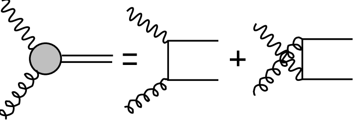
FIG. 2.:

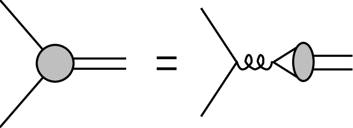
FIG. 3.:

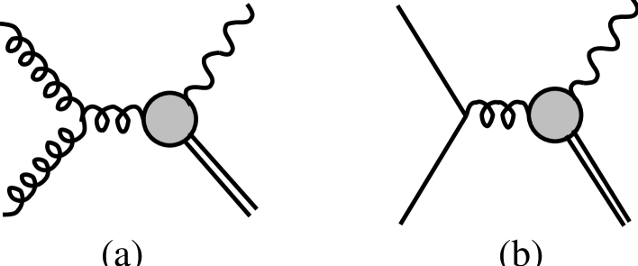
FIG. 4.:

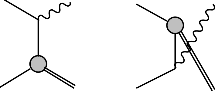
FIG. 5.:

FIG. 6.:

FIG. 7.:

FIG. 8.:

REFERENCES

• [1] E. L.Β Berger and D.Β Jones, Phys. Rev. D23 (1981) 1521.
• [2] R.Β Baier and R.Β RΓΌckl, Z. Phys. C19 (1983) 251.
• [3] E.Β Braaten and T. C.Β Yuan, Phys. Rev. Lett. 71 (1993) 1673.
• [4] E.Β Braaten, M. A.Β Doncheski, S. Fleming and M. L. Mangano, Phys. Lett. B333 (1994) 548.
• [5] D. P.Β Roy and K.Β Sridhar, Phys. Lett. B339 (1994) 141.
• [6] M. Cacciari and M.Β Greco, Phys. Rev. Lett. 73 (1994) 1586.
• [7] The CDF Collaboration, Fermilab-Conf-94/136-E (1994), unpublished.
• [8] E.Β Braaten and S.Β Fleming, Phys. Rev. Lett. 74 (1995) 3327.
• [9] P. Cho, A. K. Leibovich, Phys. Rev. D53 (1996) 150.
• [10] P. Cho, A. K. Leibovich, Phys. Rev. D53 (1996) 6203.
• [11] The CDF collaboration, Fermilab-Conf-94/221-E (1994).
• [12] S. Fleming and I. Maksymyk, Phys. Rev. D54 (1996) 3608; MADPH-95-922, UTTG-13-95, hep-ph/9512320.
• [13] P. Cho and M.B. Wise, Phys. Lett. B346, 129 (1995).
• [14] E.Β Braaten and Y.-Q.Β Chen, Phys. Rev. Lett. 76 (1996) 730.
• [15] P. Ko, Jungil Lee and H. S. Song, Phys. Rev. D53 (1996) 1409.
• [16] P. Ko, Jungil Lee and H. S. Song, Phys. Rev. D54 (1996) 4312.
• [17] K. Β Cheung, W.-Y. Keung and T. C. Yuan, Phys. Rev. Lett. 76 (1996) 877.
• [18] P. Cho, Phys. Lett. B368 (1996) 171.
• [19] S. Baek, P. Ko, Jungil Lee and H. S. Song, hep-ph/9607236.
• [20] M. Cacciari and M. KrΓ€mer, Phys. Rev. Lett. 76 (1996) 4128.
• [21] J. Amundson, S. Fleming and I. Maksymyk, UTTG-10-95, MADTH-95-914, hep-ph/9601298.
• [22] M. Cacciari and M. KrΓ€mer, hep-ph/9609500.
• [23] K. Cheung, W.-Y. Keung and T. C. Yuan, Phys. Rev. D54 (1996) 929.
• [24] E. Braaten, S. Fleming and T. C. Yuan, OHSTPY-HEP-T-96-001, hep-ph/9602374.
• [25] E. Braaten and Y-.Q. Chen, Phys. Rev. D54, 3216 (1996).
• [26] S. Fleming, O. F. Hernandez, I. Maksymyk, H. Nadeau, hep-ph/9608413.
• [27] M. Beneke and I. Z. Rothstein, Phys. Lett. B372, 157 (1996); M. Beneke and I. Z. Rothstein, Phys. Rev. D54, 2005 (1996).
• [28] M. Drees and C. S. Kim, Z.Β Phys. C53 (1992) 673.
• [29] C. S.Β Kim and E.Β Reya, Phys. Lett. B300 (1993) 298.
• [30] M. A.Β Doncheski and C. S. Kim, Phys. Rev. D49 (1994) 4463.
• [31] L.Β Antoniazzi et al., Phys. Rev. Lett. 70 (1993) 383.
• [32] C.Β Kourkoumelis et al., Phys. Lett. B 81 (1979) 405.
• [33] E. L.Β Berger and K.Β Sridhar, Phys. Lett. B317 (1993) 443.
• [34] D. P.Β Roy and K.Β Sridhar, Phys. Lett. B341 (1995) 413.
• [35] G. T. Bodwin, E. Braaten and G. P. Lepage, Phys. Rev. D51 (1995) 1125.
• [36] A.D. Martin, R.G. Roberts and W.J. Stirling, Phys. Rev. D 50, 6734 (1994).
• [37] H. Lai et al., Phys. Rev. D 51, 4763 (1995).
• [38] M. Cacciari, M. Greco and M. KrΓ€mer , hep-ph/9611324.