hep-ph/9610271

SISSA/107/96/EP

IOA-04-96

THRESHOLD EFFECTS AND RADIATIVE ELECTROWEAK SYMMETRY BREAKING IN $SU(5)$ EXTENSIONS OF THE MSSM.
A.Dedes⁽¹⁾, A.B.Lahanas⁽²⁾, J.Rizos⁽³⁾ and K.Tamvakis^(1)
(1)Division of Theoretical Physics, Physics Department,
University of Ioannina, GR-45110, Greece
⁽²⁾University of Athens, Physics Department, Nuclear and Particle Physics Section,
Ilissia, GR-157 71 Athens, Greece
⁽³⁾International School for Advanced Studies, SISSA,
Via Beirut 2-4, 34013 Trieste, Italy

Abstract
We make a complete analysis of radiative symmetry breaking in the MSSM and its $SU(5)$ extensions including low- and high-energy threshold effects in the framework of the two-loop renormalization group. In particular, we consider minimal $SU(5)$, the missing-doublet $SU(5)$, a Peccei-Quinn invariant version of $SU(5)$ as well as a version with light adjoint remnants. We derive permitted ranges for the parameters of these models in relation to predicted $\alpha_{s}$ and $M_{G}$ values within the present experimental accuracy. The parameter regions allowed under the constraints of radiative symmetry breaking, perturbativity and proton stability, include the experimentally designated domain for $\alpha_{s}$. In the case of the minimal $SU(5)$, the values of $\alpha_{s}$ obtained are somewhat large in comparison with the experimental average. The missing-doublet $SU(5)$, generally, predicts smaller values of $\alpha_{s}$. In both versions of the missing-doublet, the high energy threshold effects on $\alpha_{s}$ operate in the opposite direction than in the case of the minimal model, leading to small values. In the case of the Peccei-Quinn version however the presence of an extra intermediate scale allows to achieve an excellent agreement with the experimental $\alpha_{s}$ values. Finally, the last considered version, with light remnants, exhibits unification of couplings at string scale at the expense however of rather large $\alpha_{s}$ values.

October 1996

  E-mails : adedes@cc.uoi.gr, alahanas@atlas.uoa.gr, rizos@susy.he.sissa.it, tamvakis@cc.uoi.gr

1. Introduction

Supersymmetric unification, in the framework of supersymmetric grand unified theories (SUSY GUT’s) [1], or Superstrings [2], is in good agreement [3] [4] with the low energy values of the three gauge couplings, known to the present experimental accuracy, as well as with available bounds on the stability of the proton. The effective low energy theory resulting from such a framework is a supersymmetric $SU(3)_{c}\times SU(2)_{L}\times U(1)_{Y}$, model with softly broken supersymmetry. The simplest model of that class is the minimal extension of the standard model (MSSM) [1]. A most appealing feature realized in the MSSM is the breaking of the electroweak symmetry through radiative corrections [5]. The Higgs boson mass squared parameters, although positive definite at high energies, are radiatively corrected, as can be most easily studied by the use of the renormalization group, yielding a negative mass squared eigenvalue at low energies which triggers electroweak symmetry breaking [6] [7].

In the present article we study the radiative breaking of electroweak symmetry in the framework of $SU(5)$ SUSY GUTs. In addition to the standard low energy inputs ($\alpha_{EM}$, $G_{F}$, $M_{Z}$, …) and the soft breaking parameters ($M_{o}$, $M_{1/2}$, $A_{o}$), we have the thresholds of the superheavy particles parametrized in terms of at least two more parameters ($M_{\Sigma}$, $M_{H_{c}},...$ )  . Our output includes the strong coupling $\alpha_{s}$ and the unification scale $M_{G}$, as well as the complete spectrum of new particles. The predicted strong coupling values can depend strongly on the high energy thresholds. Thus, our analysis discriminates between the various GUT models.

Our basic low energy inputs are the boundary values of the gauge couplings in the $\overline{DR}$ scheme [8] $\hat{\alpha}_{1}\equiv\alpha_{1}(M_{Z})|_{\overline{DR}}$ and $\hat{\alpha}_{2}\equiv\alpha_{2}(M_{Z})|_{\overline{DR}}$. Their values can be determined in terms of the Fermi constant $G_{F}=1.16639\times 10^{5}$ GeV^-2, the Z-boson mass $M_{Z}=91.1884\pm 0.0022$ GeV [9], the electromagnetic coupling $\alpha_{EM}^{-1}=137.036$, the bottom quark mass $m_{b}=5$ GeV, the tau mass $m_{\tau}=1.777$ GeV, and the top quark mass. We can write down the following formulas,

$$\hat{\alpha}_{1}^{-1} = \frac{3}{5}\alpha_{EM}^{-1}\,cos^{2}\theta\,(1-\Delta_{\gamma}+\frac{\alpha_{EM}}{2\pi}\ln(\frac{M_{S}}{M_{Z}}))$$ (1)

$$\hat{\alpha}_{2}^{-1} = \alpha_{EM}^{-1}\,sin^{2}\theta\,(1-\Delta_{\gamma}+\frac{\alpha_{EM}}{2\pi}\ln(\frac{M_{S}}{M_{Z}}))$$ (2)

where $\Delta_{\gamma}$=0.0682$\pm$0.0007 [10] includes the light quark and lepton contributions, and the $\overline{DR}$ mixing angle is given by

$$sin^{2}\theta=\frac{1}{2}\{1-[1-\frac{4\pi\alpha_{EM}}{\sqrt{2}G_{F}M_{Z}^{2}(1-\Delta r)}]^{\frac{1}{2}}\}$$ (3)

The quantity $\Delta r$ will be given below. The scale $M_{S}$ appearing in (1) and (2) is not a physical scale but a convenient parametrization for the contribution of all sparticle and heavy particles $(W,t,H^{+})$, defined as

$$M_{S}=\frac{M_{W}^{-7}M_{t}^{\frac{16}{9}}M_{H^{+}}^{\frac{1}{3}}M_{\tilde{t}_{1}}^{\frac{4}{9}}M_{\tilde{t}_{2}}^{\frac{4}{9}}M_{\tilde{u}_{1,2}}^{\frac{8}{9}}M_{\tilde{u}^{c}_{1,2}}^{\frac{8}{9}}M_{\tilde{b}_{1}}^{\frac{1}{9}}M_{\tilde{b}_{2}}^{\frac{1}{9}}M_{\tilde{d}_{1,2}}^{\frac{2}{9}}M_{\tilde{d}^{c}_{1,2}}^{\frac{2}{9}}M_{\tilde{\tau}_{1}}^{\frac{1}{3}}M_{\tilde{\tau}_{2}}^{\frac{1}{3}}M_{\tilde{e}_{1,2}}^{\frac{2}{3}}M_{\tilde{e}^{c}_{1,2}}^{\frac{2}{3}}M_{\tilde{\chi}_{1}}^{\frac{4}{3}}M_{\tilde{\chi}_{2}}^{\frac{4}{3}}}{M_{Z}^{\frac{19}{9}}}$$ (4)

An additional useful parametrization scale $\tilde{M_{S}}$, relevant to the strong coupling constant ${\alpha}_{s}$, is

$$\tilde{M_{S}}=\frac{M_{t}^{\frac{2}{3}}M_{\tilde{t}_{1}}^{\frac{1}{6}}M_{\tilde{t}_{2}}^{\frac{1}{6}}M_{\tilde{u}_{1,2}}^{\frac{1}{3}}M_{\tilde{u}^{c}_{1,2}}^{\frac{1}{3}}M_{\tilde{b}_{1}}^{\frac{1}{6}}M_{\tilde{b}_{2}}^{\frac{1}{6}}M_{\tilde{d}_{1,2}}^{\frac{1}{3}}M_{\tilde{d}^{c}_{1,2}}^{\frac{1}{3}}M_{\tilde{g}}^{2}}{M_{Z}^{\frac{11}{3}}}$$ (5)

The quantity $\Delta r$ appearing in Eq. (3) can be written as [11],

$$\Delta r=\Delta_{\gamma}-\frac{\alpha_{EM}}{2\pi}\log\frac{M_{S}}{M_{Z}}-\frac{\Pi_{ZZ}(M_{Z}^{2})}{M_{Z}^{2}}+\frac{\Pi_{WW}(0)}{M_{W}^{2}}+\Delta_{SM}+\delta\rho^{QCD}+\delta\rho^{HIGGS}$$ (6)

$\Pi_{ZZ}$ and $\Pi_{WW}$ stand for the Z and W self-energies calculated using dimensional reduction. The quantity $\Delta_{SM}$ stands for Standard Model vertex+box corrections and is given by [12],

$$\Delta_{SM}=\frac{\alpha_{EM}}{4\pi sin^{2}\theta}\{6+\frac{\log{cos^{2}\theta_{W}}}{sin^{2}\theta_{W}}[\frac{7}{2}-\frac{5sin^{2}\theta_{W}}{2}-sin^{2}\theta(5-\frac{3cos^{2}\theta_{W}}{2cos^{2}\theta})]\}$$ (7)

In the last formula, by definition $cos^{2}\theta_{W}=\frac{M_{W}^{2}}{M_{Z}^{2}}$. The pole mass of W-gauge boson in (4) is related to $M_{Z}$ by $M_{W}^{2}=M_{Z}^{2}\,\rho\,cos^{2}\theta$ where the $\rho$ parameter is given by,

$$\rho=1-\frac{\Pi_{WW}(M_{W}^{2})}{M_{W}^{2}}+\frac{\Pi_{ZZ}(M_{Z}^{2})}{M_{Z}^{2}}+2-loop\,finite\,corrections.$$ (8)

We have explicitly written in (6) the 2-loop corrections due to QCD and the Higgs calculated in reference [13].

The low energy value of the strong coupling constant considered as an output is given by the formula [14],

$$\alpha_{s}^{-1}\equiv\alpha_{s}^{-1}(M_{Z})|_{\overline{MS}}=\hat{\alpha}_{3}^{-1}(M_{Z})|_{\overline{DR}}+\frac{1}{4\pi}-\frac{1}{2\pi}\ln{\frac{\tilde{M_{S}}}{M_{Z}}}$$ (9)

The current experimental values of $\alpha_{s}$ at Z-pole extracted from QCD experiments with various methods are obtained in Table I [9]. R refers to the ratio of cross sections or partial widths to hadrons versus leptons and the values of strong coupling are in $\overline{MS}$ renormalization scheme. The average value of $\alpha_{s}$ given in Ref.[9] is $\alpha_{s}(M_{Z})=0.118\pm 0.003$.

The values (1),(2) will serve as low energy boundary conditions for the corresponding two-loop renormalization group equations. As a high energy boundary conditions for the gauge couplings we shall impose unification at a scale $M_{G}$,

$$\hat{\alpha}_{1}(M_{G})=\hat{\alpha}_{2}(M_{G})=\hat{\alpha}_{3}(M_{G})\equiv\alpha_{G}$$ (10)

Note that when we depart from the minimal supersymmetric extension of the Standard Model and consider $SU(5)$ extensions of it the effect of the superheavy particles with masses around the unification scale $M_{G}$ has to be taken into account in the evolution of the gauge couplings.

Table I: Values of $\alpha_{s}(M_{Z})$ extracted from QCD experiments

The soft supersymmetry breaking is represented by four parameters $M_{o}$, $M_{1/2}$, $A_{o}$ and $B_{o}$ of which we shall consider only the first three as input parameters and treat $B(M_{Z})$, as well as the Higgs mixing parameter $\mu$, as determined by the 1-loop minimization equations,

$$sin2\beta = -\frac{2B\mu}{\overline{m}_{1}^{2}+\overline{m}_{2}^{2}}$$ (11)

$$\frac{1}{2}(M_{Z}^{2}+\Pi_{ZZ}(M_{Z}^{2})) = \frac{\overline{m}_{1}^{2}-\overline{m}_{2}^{2}tan^{2}\beta}{tan^{2}\beta-1}$$ (12)

where $\overline{m}_{i}^{2}\equiv m_{H_{i}}^{2}+\mu^{2}+\frac{\partial(\Delta V_{1-loop})}{\partial\upsilon_{i}^{2}}$. Note that cases in which the above two equations are not satisfied, and thus radiative symmetry breaking does not occur, are rejected. The parameter $\beta\equiv tan^{-1}(\frac{\upsilon_{2}}{\upsilon_{1}})$ is defined at $M_{Z}$. $M_{Z}$ in (12) denotes the experimental Z-boson mass. Thus supersymmetry breaking is parametrized with the input parameters $M_{o}$, $M_{1/2}$, $A_{o}$, $\beta(M_{Z})$ and $sign\mu(M_{Z})$. We shall take the simplest of boundary conditions at $M_{G}$ assuming universality,

$$m_{i}(M_{G})=M_{o}\,\,,\,\,M_{i}(M_{G})=M_{1/2}\,\,,\,\,A_{i}(M_{G})=A_{o}$$ (13)

We shall employ the full coupled system of 2-loop renormalization group equations [15] evolved from $M_{G}$ down to low energies. Since our purpose is to study the effect of high energy thresholds in various extensions of $SU(5)$ it will be sufficient to obtain the parameter $M_{S}$ and $\tilde{M_{S}}$, appearing in the boundary values of the low energy gauge couplings, by calculating the sparticle masses in the step approximation [16]. However, we shall introduce finite part contributions whenever they are a priori expected to be large [17], such as $QCD$ corrections to the top and gluino masses for instance etc.

Following the Particle Data Group [9] our basic experimental constraints on supersymmetric masses as well as Higgs boson masses are shown in Table II. These limits, impose stringent bounds on the extracted values of $\alpha_{s}(M_{Z})$ and on heavy high energy masses as we will see later.

TABLE II
$Particle\>\;\;\;\;\;\;\;\;\;\>\;\;\;\;\;\;\;\;\;\;\;\;\;\;\;\;\;\;Bound(GeV)$
Neutralinos
$m_{\chi_{1}^{o}}$ (LSP)	$>$23
$m_{\chi_{2}^{o}}$	$>$52
$m_{\chi_{3}^{o}}$	$>$84
$m_{\chi_{4}^{o}}$	$>$127
Charginos
$m_{\chi_{1}^{c}}$	$>$45.2
$m_{\chi_{2}^{c}}$	$>$99
Sneutrino
$m_{\tilde{\nu}}$	$>$41.8
Charged Sleptons
$m_{\tilde{e},\tilde{\mu},\tilde{\tau}}$	$>$45
Squarks
$m_{\tilde{q}}$	$>$224
Gluino
$m_{\tilde{g}}$	$>$154
Higgs Bosons
$m_{h}$	$>$44
$m_{A}^{o}$	$>$24.3
$m_{H}^{\pm}$	$>$40

Table II: Experimental bounds on supersymmetric particles and Higgs Bosons

The purpose of the present paper is to analyze the effect of high energy thresholds on unification predictions in the various $SU(5)$ extensions of the MSSM. Our goal is to complete previous existing analyses which either have not incorporated the constraints imposed by radiative symmetry breaking or have not considered the full range allowed for GUT parameters. In our consideration of supersymmetric versions of $SU(5)$ we have to take into account the constraints imposed by proton decay into $K^{+}\overline{\nu}_{\mu}$ through dimension 5 operators. Assuming that this is the dominant process the proton lifetime is [18][19][20]

$$\tau(p\longrightarrow K^{+}{\overline{\nu}}_{\mu})=6.9\times 10^{31}yrs|\frac{0.003GeV^{3}\,0.67\,\sin(2\beta)\,M_{H_{c}}\,TeV^{-1}}{\beta_{n}\,A_{S}(1+y^{tK})\,10^{17}GeV\,[f(\tilde{u},\tilde{d})+f(\tilde{u},\tilde{e})]}|^{2}$$ (14)

where $M_{H_{c}}$ is the effective colour triplet mass in GeV,$\beta_{n}\sim(0.003-0.03)GeV^{3}$, $|1+y^{tK}|\geq 0.4$, and $A_{S}=(\frac{\alpha_{1}(M_{Z})}{\alpha_{5}(M_{G})})^{\frac{7}{99}}(\frac{\alpha_{3}(M_{Z})}{\alpha_{5}(M_{GUT})})^{-\frac{4}{9}}$. The function $f(x,y)$ is defined as

$$f(x,y)=m_{\tilde{w}}\frac{1}{x^{2}-y^{2}}(\frac{x^{2}}{x^{2}-m_{\tilde{w}}^{2}}\ln(\frac{x^{2}}{m_{\tilde{w}}^{2}})-\frac{y^{2}}{y^{2}-m_{\tilde{w}}^{2}}\ln(\frac{y^{2}}{m_{\tilde{w}}^{2}})\,)$$ (15)

and masses are in GeV. The current experimental limit is

$$\tau(p\longrightarrow K^{+}{\overline{\nu}}_{\mu})\geq 10^{32}yrs$$ (16)

In what follows, we choose the most conservative values of $\beta_{n}$ and $|1+y^{tK}|$ which are $0.003GeV^{3}$ and $0.4$ respectively.

An additional constraint that will be imposed is the absence of Landau poles on the dimensionless couplings of the theory, or equivalently the validity of perturbation theory (perturbativity) of those couplings above $M_{G}$ and up to the Planck scale. Although this is in general not a severe constraint, it should be taken into account in the cases of extended versions of $SU(5)$ due to the existence of a large number of massless particles above $M_{G}$ (see for instance Fig. 3c). This constraint is implemented through the numerical solution of the 1-loop RG equations for the Yukawa couplings of $SU(5)$ above $M_{G}$ (see Appendix).

2. Minimal SU(5)

The standard superpotential [21] in the minimal $SU(5)$ is

$$\cal W = \frac{1}{2}M_{1}Tr(\Sigma^{2})+\frac{1}{3}\lambda_{1}Tr(\Sigma^{3})+M_{2}\overline{H}H+\lambda_{2}\overline{H}\Sigma H$$ (17)

$$+ \sqrt{2}Y_{(d)}^{ij}\Psi_{i}\phi_{j}\overline{H}+\frac{1}{4}Y_{(u)}^{ij}\Psi_{i}\Psi_{j}H\;\;\;\;\;\;i,j=1..3$$

$SU(5)$ is spontaneously broken to $SU(3)\times SU(2)\times U(1)$ when the adjoint Higgs $\Sigma$ develops a v.e.v in the direction $<\Sigma>\equiv V\,Diag(2,2,2,-3,-3)$. The resulting superheavy masses are ,

$$M_{V}=5g_{5}V\,\,,\,\,M_{H_{c}}=5\lambda_{2}V\,\,,\,\,M_{\Sigma}=5\lambda_{1}V$$ (18)

We have imposed the usual fine-tuning condition $M_{2}=3\lambda_{2}V$ that gives massless isodoublets of $H$,$\overline{H}$. The mass $M_{\Sigma}$ stands for the mass of the surviving colour-octet and isotriplet parts of $\Sigma$. The leading contribution of these masses to the beta function coefficients of the three gauge couplings $\frac{dg_{i}}{dt}=\frac{g_{i}^{3}(b_{i}+\Delta b_{i})}{16\pi^{2}},i=1...3$, $t=ln(\frac{Q}{M_{G}})$, $(b_{3},b_{2},b_{1})=(-3,1,\frac{33}{5})$ is

$$\Delta b_{3} = 3\theta(Q^{2}-M_{\Sigma}^{2})+\theta(Q^{2}-M_{H_{c}}^{2})-4\theta(Q^{2}-M_{V}^{2})\}$$ (19)

$$\Delta b_{2} = 2\theta(Q^{2}-M_{\Sigma}^{2})-6\theta(Q^{2}-M_{V}^{2})$$ (20)

$$\Delta b_{1} = \frac{2}{5}\theta(Q^{2}-M_{H_{c}}^{2})-10\theta(Q^{2}-M_{V}^{2})$$ (21)

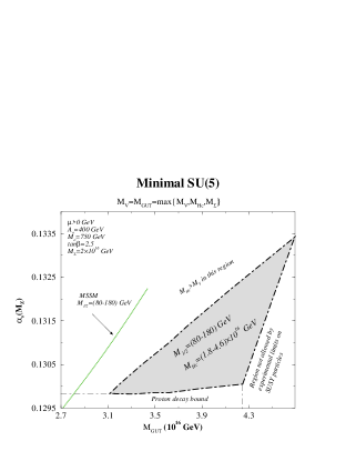
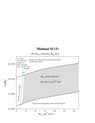
Figure 1: (a),(b) $\alpha_{s}(M_{Z})$ versus $M_{G}$ when $M_{H_{c}}$, $M_{\Sigma}$, respectively are varied.

Demanding perturbativity up to $\frac{M_{P}}{\sqrt{8\pi}}\simeq 2.4\times 10^{18}GeV$ for the couplings appearing in (17), we are led after numerically integrating the coupled system of $SU(5)$ renormalization group equations, to the inequalities

$$\lambda_{1}<1.4\,\,\,,\lambda_{2}<1.5\,\,\,,Y_{t}<1.5\,\,\,,Y_{b}<1.4$$ (22)

at $M_{G}$. Note that although in general

$$M_{G}=max\{M_{V},M_{H_{c}},M_{\Sigma}\}\,\,\,\,,$$ (23)

only the case $M_{G}=M_{V}$ can be realized under the combined constraints in our analyses. The case in which all superheavy masses are equal although allowed by the bounds given in Eq. (22) is the well studied case of the MSSM. In the context of the $SU(5)$ this requires the couplings $\lambda_{1,2},\ g_{5}\,$ to be fine tuned according to (18).

Our standard outputs are the values of the strong coupling, $\alpha_{s}(M_{Z})$, and the scale $M_{G}$ where the couplings meet. The input values of $M_{o}$ , $M_{1/2}$ and $A_{o}$ are always taken to be smaller than $1$ TeV. It must be noted that in the figures we have chosen input values such that the acceptable region in the ($\alpha_{s}$-$M_{G}$) plane is the optimum one in the following sence: We vary one parameter at a time while we keep the others constant. This is done for every input parameter, until we reach the maximum acceptable area. In the figures shown, we have adopted for the mass of the top quark an average value of the CDF and D$\O$ [22] experimental results, $m_{t}=180$ GeV. Note also that, variation of $\pm 5$GeV in $m_{t}=180$GeV results in $\pm 0.0005$ and $\pm 0.08\times 10^{16}$GeV on $\alpha_{s}$ and $M_{G}$ respectively. In addition, a variation of $\pm 0.0007$ in the central value of $\Delta_{\gamma}$ gives variation of $\mp 0.001$ and $\mp 0.5\times 10^{16}$GeV on $\alpha_{s}$ and $M_{G}$ respectively.

The shaded areas of Figures 1a and 1b represent the allowed parameter space for the outputs $\alpha_{s}(M_{Z})$ and $M_{G}$. The results do not depend significantly on $M_{o}$ and $A_{o}$ which have been chosen to have the representative values shown. The allowed area shrinks with increasing $tan\beta$ due to the proton decay bound. For smaller values the allowed area shrinks because of the perturbativity of $Y_{t}(M_{G})$ and the constraint from radiative symmetry breaking. In Figure 1a we have chosen a characteristic value for $M_{\Sigma}$ while we have varied $M_{H_{c}}$ through its allowed range of values $(1.8-4.6)\times 10^{16}$ GeV. Analogously in Figure 1b we have taken $M_{H_{c}}=3\times 10^{16}$ GeV, while we have varied $M_{\Sigma}$ through the range of values $(0.1-2)\times 10^{16}$ GeV. The values of $\alpha_{s}$ obtained are in general too large in comparison with the average experimental value. Making a parameter search, we conclude that the lowest possible value that we can reach in this model is close to $\simeq 0.130$. Nevertheless, there are processes (Table I) whose determined $\alpha_{s}$ agrees in a limiting sense with the smallest values in Fig. 1. It should be noted that the effect of high energy thresholds has made the access to the smaller values of $\alpha_{s}$ worse than in the case of the MSSM. The general dependence of $\alpha_{s}$ is that it increases with increasing $M_{H_{c}}$ while it decreases with increasing $M_{\Sigma}$.

3. Missing Doublet Model

Let us now consider an extended version of the $SU(5)$ known as the Missing Doublet Model. This model [23], constructed in order to avoid the numerical fine-tuning required in the minimal $SU(5)$, has instead of the adjoint GUT Higgs a Higgs field in the 75 representation as well as an extra pair of Higgses in the ${\bf{50}}+{\bf{\overline{50}}}$ representation. The superpotential is

$$\cal W = M_{1}Tr(\Sigma^{2})+\frac{1}{3}\lambda_{1}Tr(\Sigma^{3})+\lambda_{2}H\Sigma\Theta+\overline{\lambda}_{2}\overline{H}\Sigma\overline{\Theta}+M_{2}\overline{\Theta}\Theta$$ (24)

$$+ \frac{1}{4}Y_{(u)}^{ij}\Psi_{i}\Psi_{j}H+\sqrt{2}Y_{(d)}^{ij}\Psi_{i}\phi_{j}\overline{H}\;\;\;\;\;\;i,j=1..3$$

Since the $\Theta$,$\overline{\Theta}$ do not contain any isodoublets, only the coloured triplets obtain masses while the isodoublets in $H$,$\overline{H}$ stay massless. The v.e.v

$$\Sigma^{CD}_{AB}=V((\delta_{c})^{C}_{A}(\delta_{c})^{D}_{B}+2(\delta_{w})^{C}_{A}(\delta_{w})^{D}_{B}-\frac{1}{2}\delta^{C}_{A}\delta^{D}_{B}-(C\leftrightarrow D))$$ (25)

leads to the masses

$$M(3,1,\frac{5}{3}) = \frac{4}{5}M_{\Sigma}\,\,\,,M(8,1,0)=\frac{M_{\Sigma}}{5}\,\,\,,M(8,3,0)=M_{\Sigma}$$

$$M(6,2,\frac{5}{6}) = \frac{2}{5}M_{\Sigma}\,\,\,,M(1,1,0)=\frac{2}{5}M_{\Sigma}$$

for the remnants of 75. The assignment of the quantum numbers refers to the group $SU(3)\times SU(2)\times U(1)$ . We shall assume that the parameter $M_{2}$ is larger than the GUT scale possibly of the order of the Planck mass. Otherwise perturbativity, as can be easily seen, cannot be fulfilled. The charge - $1\over 3$ colour triplets in $H$,$\overline{H}$ and $\Theta$,$\overline{\Theta}$ will give one supermassive combination of mass $M_{H_{c^{\prime}}}\simeq O(M_{2})$ and a light combination of mass

$$M_{H_{c}}\simeq\frac{9}{100}(\frac{32\lambda_{2}\overline{\lambda}_{2}}{\lambda_{1}^{2}})(\frac{M_{\Sigma}^{2}}{M_{2}})$$ (26)

The mass parameter $M_{\Sigma}$ is related to the vector boson mass through

$$\frac{M_{\Sigma}}{M_{V}}=\frac{5M_{1}}{2\sqrt{15}g_{5}V}=\frac{(10/3)\lambda_{1}}{2\sqrt{15}g_{5}}=\frac{1}{3}\sqrt{\frac{5}{3}}(\frac{\lambda_{1}}{g_{5}})$$ (27)

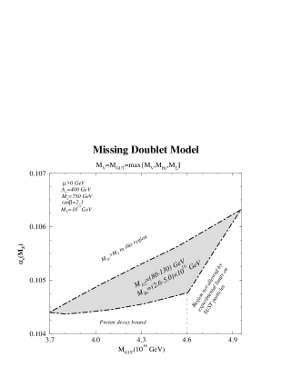
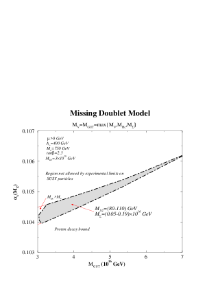
Figure 2: (a),(b) $\alpha_{s}(M_{Z})$ versus $M_{G}$ when $M_{H_{c}}$, $M_{\Sigma}$, respectively are varied.

The modifications in the beta function coefficients are,

$$\Delta b_{3} = -4\theta(Q^{2}-M_{V}^{2})+9\theta(Q^{2}-M_{\Sigma}^{2})+\theta(Q^{2}-0.8^{2}M_{\Sigma}^{2})$$ (28)

$$+ 10\theta(Q^{2}-0.4^{2}M_{\Sigma}^{2})+3\theta(Q^{2}-0.2^{2}M_{\Sigma}^{2})+\theta(Q^{2}-M_{H_{c}}^{2})+\theta(Q^{2}-M_{H_{c^{\prime}}}^{2})$$

$$+ 34\theta(Q^{2}-M_{2}^{2})$$

$$\Delta b_{2} = -6\theta(Q^{2}-M_{V}^{2})+16\theta(Q^{2}-M_{\Sigma}^{2})+6\theta(Q^{2}-0.4^{2}M_{\Sigma}^{2})$$ (29)

$$+ 35\theta(Q^{2}-M_{2}^{2})$$

$$\Delta b_{1} = -10\theta(Q^{2}-M_{V}^{2})+10\theta(Q^{2}-0.8^{2}M_{\Sigma}^{2})+10\theta(Q^{2}-0.4^{2}M_{\Sigma}^{2})$$ (30)

$$+ \frac{2}{5}\theta(Q^{2}-M_{H_{c}}^{2})+\frac{2}{5}\theta(Q^{2}-M_{H_{c^{\prime}}}^{2})+\frac{173}{5}\theta(Q^{2}-M_{2}^{2})$$

Perturbativity above $M_{G}$, as in the case of minimal $SU(5)$, leads us to the extra constraints at $M_{G}$

$$\lambda_{1}<0.18\,\,\,\,,Y_{t}<1.6\,\,\,\,,Y_{b}<1.5$$ (31)

In this model, we obtain a stronger constraint on $\lambda_{1}$, and consequently on $M_{\Sigma}$, due to the fact that now we have a larger dimensional representation (75).

Note that the model as it stands does not contain any $\mu$-term. We assume, however, that a $\mu$-term is generated through an independent mechanism [24].

In Figures 2a and 2b it can be seen that the values of $\alpha_{s}$ obtained are much smaller than the average experimental value. We should note that $\alpha_{s}$ is pushed towards smaller values due to the splittings within 75 that give a large correction in the opposite direction than in the case of the minimal model [23]. The maximum value of $\alpha_{s}$ that we are able to obtain in the Missing Doublet Model, is approximately $\simeq 0.106$. As we can see from Table I, there are still QCD processes, where the values of $\alpha_{s}$ are in agreement with the results of the missing doublet model. The heavy masses $M_{H_{c}}$ and $M_{\Sigma}$ are constrained to be in the regions $(2.6-5.0)\times 10^{16}$ GeV and $(0.05-0.19)\times 10^{16}$ GeV respectively. Due to the fact that the extracted values of $\alpha_{s}$ in MSSM are greater than 0.125 (for the inputs of Figs 2a,b), we do not display in Figures 2a and 2b the corresponding MSSM plane. Experimental limits on LSP (see Table II) puts a lower bound on the universal soft gaugino masses such that $M_{1/2}\geq 80$ GeV.

4. Peccei-Quinn symmetric missing-doublet model

The problem of proton decay through D=5 operators that is present in the minimal $SU(5)$ model provided strong motivation to construct versions of $SU(5)$ with a Peccei-Quinn symmetry[25] that naturally suppresses these operators by a factor proportional to the ratio of the Peccei-Quinn breaking scale over the GUT scale [26]. A Peccei-Quinn version of the missing doublet $SU(5)$ model requires the doubling of ${\bf 5}+{\bf{\overline{5}}}$ and ${\bf 50}+{\bf{\overline{50}}}$ representations. The relevant superpotential terms which must be added to the previous superpotential are,

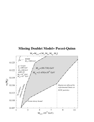
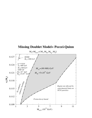
Figure 3: (a),(b),(c) $\alpha_{s}(M_{Z})$ versus $M_{G}$ when $M_{H_{f}^{\prime}}$, $M_{H_{c}}$ and $M_{\Sigma}$ are varied.

$$\lambda_{2}H\Sigma\overline{\Theta} + \overline{\lambda}_{2}\overline{H}\Sigma\Theta+\lambda^{\prime}_{2}H^{\prime}\Sigma\overline{\Theta}^{\prime}+\overline{\lambda}^{\prime}_{2}\overline{H}^{\prime}\Sigma\Theta^{\prime}$$ (32)

$$+ M_{2}\Theta\overline{\Theta}^{\prime}+M_{2}^{\prime}\Theta^{\prime}\overline{\Theta}+\lambda_{3}P\overline{H}^{\prime}H^{\prime}$$

$P$ stands for an extra gauge singlet superfield. The charges under the Peccei-Quinn symmetry are $\Psi(\alpha/2)$, $\phi(\beta/2)$, $H(-\alpha)$, $\overline{H}^{\prime}(-\frac{\alpha+\beta}{2})$, $\overline{\Theta}(\alpha)$, $\Theta(\frac{\alpha+\beta}{2})$, $\Theta^{\prime}(-\alpha)$, $\overline{\Theta}^{\prime}(-\frac{\alpha+\beta}{2})$, $H^{\prime}(\frac{\alpha+\beta}{2})$, $\overline{H}^{\prime}(\alpha)$, $P(-(3\alpha+\beta))$. The breaking of the Peccei-Quinn symmetry can be achieved with a suitable gauge singlet system at an intermediate energy $<P>\equiv\frac{M_{H^{\prime}_{f}}}{\lambda_{3}}\sim 10^{10}-10^{12}GeV$. Assuming $M_{2}$, $M_{2}^{\prime}$ to be of the order of the Planck scale, we obtain two massive pairs of coloured triplets with masses

$$M_{H_{c}}\simeq 32\lambda_{2}\overline{\lambda}^{\prime}_{2}\frac{V^{2}}{M_{2}}\;\;\;,\;\;\;M_{\overline{H}_{c}}\simeq 32\overline{\lambda}_{2}\lambda^{\prime}_{2}\frac{V^{2}}{M_{2}^{\prime}}$$ (33)

somewhat below the GUT scale. Note that $M_{V}=2\sqrt{15}g_{5}V$. In addition we have two pairs of isodoublets one of which is massless while the other pair receives the intermediate mass $M_{H^{\prime}_{f}}$. The modifications in the renormalization group beta functions coefficients are,

$$\Delta b_{3} = -4\theta(Q^{2}-M_{V}^{2})+9\theta(Q^{2}-M_{\Sigma}^{2})+\theta(Q^{2}-0.8^{2}M_{\Sigma}^{2})$$ (34)

$$+ 10\theta(Q^{2}-0.4^{2}M_{\Sigma}^{2})+3\theta(Q^{2}-0.2^{2}M_{\Sigma}^{2})+\theta(Q^{2}-M_{H_{c}}^{2})+\theta(Q^{2}-M_{\overline{H}_{c}}^{2})$$

$$\Delta b_{2} = -6\theta(Q^{2}-M_{V}^{2})+16\theta(Q^{2}-M_{\Sigma}^{2})+6\theta(Q^{2}-0.4^{2}M_{\Sigma}^{2})$$ (35)

$$+ \theta(Q^{2}-M_{H_{f}^{\prime}}^{2})$$

$$\Delta b_{1} = -10\theta(Q^{2}-M_{V}^{2})+10\theta(Q^{2}-0.8^{2}M_{\Sigma}^{2})+10\theta(Q^{2}-0.4^{2}M_{\Sigma}^{2})$$ (37)

$$+ \frac{2}{5}\theta(Q^{2}-M_{H_{c}}^{2})+\frac{2}{5}\theta(Q^{2}-M_{\overline{H}_{c}}^{2})+\frac{3}{5}\theta(Q^{2}-M_{{H}_{f}^{\prime}}^{2})$$

Bounds, which come from perturbativity of couplings in this model, are numerically similar, to those of the previous one (see Appendix). The extra coupling $\lambda_{3}$ obeys the constraint $\lambda_{3}<2.7$ at $M_{G}$.

It is evident from figures 3 that the values of $\alpha_{s}$ obtained for the case of this model are in excellent agreement with the experiment. The range of these values $(0.107-0.140)$, covers the experimental average value of $\alpha_{s}$ and lays between the gap of the Minimal SU(5) model and the Missing Doublet model. This model possesses an additional parameter, the intermediate scale $M_{H_{f}^{\prime}}$ which increases the values of $\alpha_{s}$ when it takes lower values. The allowed range of values for $M_{1/2}$ has been increased now to 730 GeV or 900 GeV in Figure 3a and 3b respectively. For this model the allowed range for $M_{o}$ can be extended to lower values. Figure 3a and 3b have been obtained for $M_{o}=300$ GeV. Note however that still $\alpha_{s}$ does not depend significantly on $M_{o}$. In addition, $tan\beta$ can practically now take much larger values, as large as $tan\beta\sim 40$. Figures 3a, 3b and 3c have been obtained for an intermediate value $tan\beta=10$. The allowed range of values for the intermediate scale $M_{H_{f}^{\prime}}$ is $(1-450)\times 10^{10}$ GeV . Similarly $5\times 10^{14}<M_{H_{c}}<M_{G}$ and $7\times 10^{14}<M_{\Sigma}<15\times 10^{14}$ GeV . Note finally, that the grand unification scale can take values as large as the “string scale” for rather large but not excluded values of $\alpha_{s}$.

5. A version of SU(5) with light remnants

Recently there has been some activity around models with gauge group $G\times G$ with intent to bypass the known problem of k=1 superstring constructions where no adjoint Higgs can appear in the massless spectrum [27]. Vector-vector Higgses present in the spectrum of $G\times G$ can break it into $G_{diag}$. An $SU(5)\times SU(5)$ model with Higgses $Z(5,\overline{5})+\overline{Z}(\overline{5},5)$ can have renormalizable couplings only of the type $\Phi Z^{i}_{j}\overline{Z}^{j}_{i}=\Phi Tr(Z\overline{Z})$ to a singlet $\Phi$, in addition to self-couplings of singlets. Thus we could construct an analog $SU(5)$ GUT with superpotential,

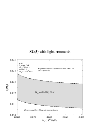
Figure 4: (a),(b) $\alpha_{s}$ and $M_{G}$ vs $M_{\Sigma}$ in SU(5) model with light remnants.

$${\cal W}=\frac{\lambda_{1}}{2}\Phi_{1}Tr(\Sigma^{2})+\frac{\lambda_{2}}{2}\Phi_{1}\Phi_{2}^{2}+\frac{\lambda_{3}}{3}\Phi_{1}^{3}$$ (38)

where $\Sigma$ is the adjoint and $\Phi_{1}$, $\Phi_{2}$ are singlets. This superpotential is invariant under $\Phi_{2}\rightarrow-\Phi_{2}$. The F-flatness conditions give, apart from $<\Sigma>=VDiag(2,2,2,-3,-3)$,

$$\Phi_{2}^{2}=-\frac{\lambda_{1}}{\lambda_{2}}(30V^{2})\,\,\,\,,\Phi_{1}=0$$ (39)

With the above superpotential the remnants of $\Sigma$, a colour octet and an isotriplet, stay massless. Nevertheless, non-renormalizable terms like

$$\Delta{\cal W}=\frac{\lambda_{4}}{M}Tr(\Sigma^{4})+\frac{\lambda_{5}}{M}(Tr(\Sigma^{2}))^{2}$$ (40)

can in principle induce a mass of order $O(\frac{V^{2}}{M})\sim 10^{14}GeV$ or smaller, depending on the actual values of $\lambda_{4}$ and $\lambda_{5}$. A higher order non-renormalizable term would induce an even smaller mass $\frac{V^{3}}{M^{2}}\sim 10^{12}GeV$. The light $\Sigma$ in this model could allow for a large $M_{G}$ close to a string unification scale and thus in such a model there would be no string unification mismatch.

We shall therefore investigate the effects of small $M_{\Sigma}$ on $\alpha_{s}$ and $M_{G}$. In order to obtain acceptably small values of $\alpha_{s}$, we choose as input value of $M_{H_{c}}$ the smallest acceptable one as it is shown in Figures 4a and 4b, since an increasing $M_{H_{c}}$ tends to increase $\alpha_{s}$. When we vary $M_{\Sigma}$ from $10^{15}$ down to $10^{13}$ GeV, we can achieve unification at $M_{G}=5\times 10^{17}$ GeV $\simeq O(M_{string})$. Decreasing $M_{\Sigma}$ further towards the intermediate scale, leads to even larger values of $\alpha_{s}$. However, the values of $\alpha_{s}$ are still rather large ($>0.131$). This excludes this particular version at least in this simple form.

6. Conclusions

In this article we have studied various supersymmetric extensions of the Standard Model based on the group $SU(5)$. The low energy precision data in conjunction with the existing experimental bounds on sparticle masses are known to impose strong constraints if radiative breaking of the electroweak symmetry is assumed. There exist several detailed studies in the literature in the framework of radiative symmetry breaking [6, 7, 10, 11, 16, 17], which however have not considered in detail the effect of the superheavy degrees of freedom included in unified schemes. In SUSY GUTs there are additional constraints one has to deal with such as the experimental bound on proton’s lifetime, the absence of Landau poles beyond the unification scale and the appearance of heavy thresholds which influence the evolution of the couplings involved. All these affect the low energy predictions. The existing analyses in this direction on the other hand [18, 19, 23, 20, 26, 27], have not systematically taken into account the effect of the low energy thresholds at the level of accuracy required by low energy precision data as was done in the previous references. Our analysis combines both and takes into account high and low energy thresholds at the accuracy required by precision experiments. In particular we have focused our attention on the extracted value of the strong coupling constant $\alpha_{s}(M_{Z})$ , the value of the unification scale $M_{G}$, as well as the restrictions imposed on the heavy masses in some unifying schemes based on the $SU(5)$. Sample results of our findings have been displayed in figures 1-4.

In the case of the minimal $SU(5)$ we found that the values of the strong coupling constant obtained are somewhat larger as compared to the average experimental value of $\alpha_{s}(M_{Z})$. Also the unification scale $M_{G}$ differs from the string unification scale by an order of magnitude if the lower values of $\alpha_{s}(M_{Z})$ obtained are assumed. Access to small values of the strong coupling constant is more difficult than in the MSSM exhibiting the influence of the superheavy degrees of freedom in a clear manner. The range of $M_{H_{c}}$ allowed in this model is somewhat limited. The Missing doublet model seems to favour small values of $\alpha_{s}(M_{Z})$, in contrast to those obtained in the MSSM and the minimal $SU(5)$ version. At the same time when $M_{G}$ increases the allowed parameter space shrinks considerably. Proton decay along with perturbativity requirements seem to put a stringent constraint on both minimal SU(5) and Missing Doublet Model (MDM). In the MDM the large splittings within $\bf{75}$ give a high energy threshold effect on $\alpha_{s}(M_{Z})$ in the opposite direction than in the case of the minimal model leading to small values. This is also the case for the Peccei-Quinn version of the MDM. However the presence of an extra intermediate scale ameliorates the situation allowing to achieve an excellent agreement with the experimental values of $\alpha_{s}(M_{Z})$. The grand unification scale can take values as large as the string scale at the expense however of having rather large values of the strong coupling constant not favoured by all experiments. If we consider the range for allowed values of $\alpha_{s}(M_{Z})$, the minimal SU(5) lays always above $.130$ while MDM lays below $.106$. The intermediate range between the two can be covered by the Peccei-Quinn version of the MDM and coincides with the allowed experimental range. Finally, the last considered version, with light $\Sigma$, exhibits unification of couplings at string scale but the values of $\alpha_{s}$ obtained are rather large, although within the errors of some experiments.

Acknowledgements

A.D. would like to thank J. Rosiek for useful conversations. A.B.L. acknowledges support by the EEC Science Program No. SCI-CT92-0792. A.D. acknowledges support from the Program $\Pi$ENE$\Delta$ 95, the EEC Human Capital and Mobility Program CHRX-CT93-0319 and the CHRX-CT93-0132 (“Flavordynamics”).

Appendix : RGE’s above $M_{G}$

The Renormalization group equations for the gauge and Yukawa couplings from $M_{GUT}$ to $\frac{M_{P}}{\sqrt{8\pi}}\simeq 2.4\times 10^{18}GeV$ in the case of minimal $SU(5)$ are [19, 20],

$$\frac{dg_{5}}{dt} = -\frac{3}{(4\pi)^{2}}g_{5}^{3}$$ (41)

$$\frac{d\lambda_{1}}{dt} = \frac{\lambda_{1}}{(4\pi)^{2}}(\frac{63}{5}\lambda_{1}^{2}+3\lambda_{2}^{2}-30g_{5}^{2})$$ (42)

$$\frac{d\lambda_{2}}{dt} = \frac{\lambda_{2}}{(4\pi)^{2}}(\frac{21}{5}\lambda_{1}^{2}+\frac{53}{5}\lambda_{2}^{2}-\frac{98}{5}g_{5}^{2}+3Y_{t}^{2}+4Y_{b}^{2})$$ (43)

$$\frac{dY_{t}}{dt} = \frac{Y_{t}}{(4\pi)^{2}}(\frac{24}{5}\lambda_{2}^{2}+9Y_{t}^{2}+4Y_{b}^{2}-\frac{96}{5}g_{5}^{2})$$ (44)

$$\frac{dY_{b}}{dt} = \frac{Y_{b}}{(4\pi)^{2}}(\frac{24}{5}\lambda_{2}^{2}+3Y_{t}^{2}+10Y_{b}^{2}-\frac{84}{5}g_{5}^{2})$$ (45)

where $t=ln(\frac{Q}{M_{P}/\sqrt{8\pi}})$.

The modification of the above system in the case of the missing doublet model is,

$$\frac{dg_{5}}{dt} = \frac{17}{(4\pi)^{2}}g_{5}^{3}$$ (46)

$$\frac{d\lambda_{1}}{dt} = \frac{\lambda_{1}}{(4\pi)^{2}}(\frac{56}{3}(8\lambda_{1})^{2}-48g_{5}^{2})$$ (47)

The other two equations for the top and bottom Yukawa coupling are derived if we set $\lambda_{2}=0$ in the eqs.(43,44) of the minimal model. Due to the fact that we have an extra pair of Higgs ${\bf{5}}$ and ${\bf{\overline{5}}}$ in the Peccei-Quinn version of the missing doublet model, the only equation that changes compared to the missing doublet model is the one for the gauge coupling which takes the form

$$\frac{dg_{5}}{dt}=\frac{18}{(4\pi)^{2}}g_{5}^{3}$$ (48)

In this model we have an extra coupling $\lambda_{3}$ whose running is given by the following renormalization group equation

$$\frac{d\lambda_{3}}{dt}=\frac{\lambda_{3}}{(4\pi)^{2}}(3\lambda_{3}^{2}-\frac{48}{5}g_{5}^{2})$$ (49)

References

[1]For reviews see:
H. P. Nilles, Phys. Rep. 110(1984)1 ;
H. E. Haber and G. L. Kane, Phys. Rep. 117(1985)75 ;
A. B. Lahanas and D. V. Nanopoulos, Phys. Rep. 145(1987)1;
H. Haber, SCIPP-92/33, TASI-92 Lectures, hep-ph/9306207;
J. L. Lopez, D. V. Nanopoulos and A. Zichichi, Prog. Part.
Nucl. Phys. 33(1994)303;
H. Baer et.al, FSU-HEP-9504401, LBL-37016 and UH-511-822-95,
hep-ph/9503479;
M. Drees and S. Martin, Report of Subgroup 2 of the DPF Working Group on
“Electroweak Symmetry breaking and Beyond the Standard Model.”,
hep-ph/9504324;
H. P. Nilles, TUM-TH-230/95, SFB-375/25, hep-ph/9511313;
J. Ellis, Invited Rapporteur Talk at the Internal Symposium on Lepton and
Photon Interactions at High Energies, Beijing, August 1995, hep-ph/9512335;
J. A. Bagger, hep-ph/9604232;
C. Csaki, Mod. Phys. Lett. A, Vol.11(1996)599.
[2]For a review see
M.Green, J.Schwarz and E.Witten
“Superstring Theory”
Cambridge U.P., Cambridge 1987.
[3]
J. Ellis, S. Kelley and D. V. Nanopoulos, Phys. Lett. B260(1991)131;
U. Amaldi, W. De Boer and M. Fürstenau,
Phys. Lett. B260(1991)447;
P. Langacker and M. Luo, Phys. Rev. D44(1991)817.
[4] P. Langacker and N. Polonsky, Phys. Rev. D47(1993)4028;
D52(1995)3081; N. Polonsky, UPR-0641-T, hep-ph/9411378.
[5] L. E. Ibañez and G. G. Ross, Phys. Lett.
110(1982)215;
K. Inoue, A. Kakuto, H. Komatsu and S. Takeshita,
Progr. Theor. Phys. 68(1982)927, 71(1984)96 ;
J. Ellis, D. V. Nanopoulos and K. Tamvakis, Phys. Lett. B121(1983)123;
L. E. Ibañez , Nucl. Phys. B218(1983)514 ;
L. Alvarez-Gaumé, J. Polchinski and M. Wise, Nucl. Phys. B221(1983)495;
J. Ellis, J.S. Hagelin, D.V. Nanopoulos and K. Tamvakis,
Phys. Lett.
B125(1983)275;
L. Alvarez-Gaumé, M. Claudson and M. Wise, Nucl. Phys. B207(1982)96;
C. Kounnas, A. B. Lahanas, D. V. Nanopoulos and M. Quiros,
Phys. Lett. B132(1983)95 , Nucl. Phys. B236(1984)438;
L. E. Ibañez and C. E. Lopez, Phys. Lett. B126(1983)54 ,
Nucl. Phys. B233(1984)511.
[6]
G. G. Ross and R. G. Roberts, Nucl. Phys. B377(1992)571;
P. Nath and R. Arnowitt , Phys. Lett. B287(1992)89;
S. Kelley, J. Lopez, M. Pois , D. V. Nanopoulos and K. Yuan ,
Phys. Lett. B273(1991)423 , Nucl. Phys. B398(1993)3;
M. Olechowski and S. Pokorski, Nucl. Phys. B404(1993)590;
M. Carena, S. Pokorski and C. E. Wagner, Nucl. Phys. B406(1993)59;
P. Chankowski, Phys. Rev. D41(1990)2873;
A.Faraggi, B.Grinstein, Nucl.Phys B422(3)1994.
[7]
G. Gamberini, G. Ridolfi and F. Zwirner, Nucl. Phys. B331(1990)331;
R. Arnowitt and P. Nath, Phys. Rev. D46(1992)3981;
D. J. Castaño, E. J. Piard and P. Ramond, Phys. Rev. D49(1994)4882;
G.L Kane, C.Kolda, L.Roszkowski and J.Wells, Phys.Rev D49(6173)1994;
V.Barger, M.S.Berger, P.Ohmann, Phys.Rev.D49(4900)1994.
[8]
W. Siegel, Phys. Lett. B84(1979)193 , D. M. Capper et al.,
Nucl. Phys. B167(1980)479;
I. Antoniadis, C. Kounnas and K. Tamvakis, Phys. Lett. B119(1982)377;
S. P. Martin and M. T. Vaughn, Phys. Lett. B318(1993)331.
[9] R.M. Barnett et al., Phys.
Rev. D54,1 (1996) ;
P. Langacker, Talk presented at SUSY-95, Palaiseau, France, May 1995,
NSF-ITP-95-140, UPR-0683T.
[10]P.H. Chankowski, Z. Pluciennik, S. Pokorski
and C.E. Vayonakis, Phys. Lett. B358(1995)264.
[11]P.H. Chankowski et al., Nucl. Phys. B417(1994)101;
P.H. Chankowski, Z. Pluciennik, S. Pokorski
Nucl. Phys. B439 (1995)23;
J. Bagger, K. Matchev, D. Pierce, Phys. Lett. B348(1995)443;
R. Barbieri, P. Giafaloni and A. Strumia, Nucl. Phys. B442(1995)461;
M. Bastero-Gil and J. Perez-Mercader, Nucl. Phys. B450(1995)21.
[12]G. Degrassi, S. Fanchiotti, A. Sirlin,
Nucl. Phys.B351(1991)49;
G. Degrassi, P. Gambino and A. Vicini, hep-ph/9603374.
[13]S. Fanchiotti, B. Kniehl and A. Sirlin, Phys.
Rev D48(1993)307;
R. Barbieri, M. Beccaria, P. Ciafaloni, G. Curci, A. Vicere, Phys. Lett.
B288(1992)95;
W. Hollik, Munich preprint MPI-Ph/93-21, April 1993;
A. Djouadi, C. Verzegnassi, Phys. Lett. B195(1987)265;
A. Djouadi, Nuovo Cimento A100(1988)357;
B.A. Kniehl, J.H. Kuhn, R.G. Stuart, Phys. Lett. B214(1988)621;
B.A. Kniehl, Nucl. Phys. B347(1990)86;
F.A. Halzen, B.A. Kniehl, Nucl. Phys. B353(1991)567.
[14]L. Hall, Nucl. Phys. B178(1981)75.
[15]
S. P. Martin and M. T. Vaughn, Phys.Rev. D50(1994)2282;
Y.Yamada, Phys.Rev D50(1994)3537;
I. Jack and D. R. T. Jones, Phys.Lett.B333(1994)372.
[16]
A. B. Lahanas and K. Tamvakis, Phys. Lett. B348(1995)451 ;
A. Dedes, A. B. Lahanas and K. Tamvakis, Phys. Rev. D53(1996)3793.
[17]
P.H. Chankowski, S. Pokorski and J. Rosiek, Nucl. Phys. B423(1994)437;
D. Pierce, J. A. Bagger, K. Matchev and R. Zhang, hep-ph/9606211.
[18] P. Nath, A. H. Chamseddine and R. Arnowitt, Phys. Rev.
D32(1985)2348;
P. Nath, R. Arnowitt, Phys. Rev. D38(1988)1479.
[19]J.Hisano, H.Murayama and T.Yanagida, Nucl. Phys. B402(1993)46;
Phys.Rev.Lett. 69 (1992)1014;
Y. Yamada, Z. Phys. C60(1993)83;
J. Hisano, T. Moroi, K. Tobe, and T. Yanagida, Mod. Phys. Lett A10(1995)2267.
[20]B.D. Wright, hep-ph/9404217.
[21]
S. Dimopoulos, H. Georgi, Nucl. Phys. B193(1981)150;
N. Sakai, Z. Phys. C11(1981)153.
[22]
F. Abe et.al, Phys.Rev.Lett. 74(1995)2676;
S. Abach et.al, Phys.Rev.Lett.74(1995)2632.
[23]A. Masiero, D.V. Nanopoulos, K. Tamvakis and T. Yanagida,
Phys.Lett. B115(1982)380;
B. Grinstein, Nucl. Phys. B206(1982);
K. Hagiwara and Y.Yamada, Phys.Rev.Lett.70(1993)709.
[24]
J. E. Kim and H. P. Nilles, Phys. Lett. B138(1984)150;
G. F. Giudice and A. Masiero, Phys. Lett. B206(1988)480;
E. J. Chun, J. E. Kim and H.-P. Nilles, Nucl. Phys. B370(1992)105;
I. Antoniadis, E. Gava, K. S. Narain and T. R. Taylor,
Nucl.Phys.B432(1994)187;
H. P. Nilles and N. Polonsky, hep-ph/9606388.
[25]
R. Peccei and H. Quinn, Phys. Rev. Lett. 38(1977)1440.
[26]J. Hisano, T. Moroi, K. Tobe, and T. Yanagida, Phys. Lett.
B342(1995)138;
J. Hisano, TIT-HEP-307, Talk given at Yukawa International Seminar’95;
L. Clavelli and P.W. Coulter, Phys. Rev. D51(1995)3913;
J.L Lopez, D.V. Nanopoulos, Phys. Rev. D53(1996)2670.
[27]C. Bachas, C. Fabre and T. Yanagida, Phys. Lett. B370(1996)49;
R. Barbieri, G. Dvali and A. Strumia, Phys. Lett. B333(1994)79.