FINITE TEMPERATURE EFFECTIVE THEORIES

Lecture Notes, Summer School on Effective Theories and Fundamental Interactions, Erice, 1996. I describe the construction of effective field theories for equilibrium high-temperature plasma of elementary particles.

1 Motivation

High-temperature and dense matter of elementary particles appears in several areas of physics. The first and most familiar example is the Universe at the early stages of its expansion. The Big Bang theory (for reviews see, e.g. $\!{}^{{\bf?},{\bf?}}$) states that the Universe was hot and dense in the past, with a temperature ranging from a few eV up to the Planck scale $\sim M_{Pl}\sim 10^{19}$ GeV. Another place, where matter exists in extreme conditions of high densities, can be created in the laboratory. Namely, in heavy-ion collisions extended dense fireballs of nuclear matter are created, with the energy density exceeding the QCD scale $\sim 10\cdot(200\mbox{M}eV)^{4}$.

From a practical point of view, there is quite a wide area of applications of finite-temperature field theory to cosmology and laboratory experiments. The high-temperature phase transitions, typical for grand unified theories (GUTs), may be important for cosmological inflation and primordial density fluctuations. Topological defects (such as monopoles, strings, domain walls) can naturally arise at the phase transitions and influence the properties of the Universe we observe today. The first-order electroweak (EW) phase transition is a crucial element for electroweak baryogenesis; it may also play a role in the formation of the magnetic fields observed in the Universe. The QCD phase transition and properties of the quark-gluon plasma are essential for the understanding of the physics of heavy-ion collisions. The QCD phase transition in cosmology may influence the spectrum of the density fluctuations relevant to structure formation.

In most cosmological applications, the deviations from thermal equilibrium play a most important role. For example, the concentration of primordial monopoles depends a lot on the dynamics of the grand unified phase transition; the baryonic asymmetry, produced in GUTs or in the EW theory, depends on the rate of the Universe expansion or other time-dependent phenomena. The signatures of the heavy-ion collisions are greatly influenced by the non-equilibrium dynamics. The study of non-equilibrium properties of the plasma is very hard. To understand the thermal non-equilibrium better, the systems in thermal equilibrium should be completely understood. Without this understanding, we cannot even say what a deviation from thermal equilibrium is. After the structure of the ground state is found, small deviations from thermal equilibrium can be treated by this or that perturbative method.

The topic of my lecture here is the study of the equilibrium properties of the plasma at high temperatures. As we will see, even this problem in gauge theories is highly non-trivial and requires the use of effective field theory methods.

The study of dense matter is interesting in itself from a theoretical point of view. At very small temperatures and densities the plasma can be considered as a collection of weakly interacting individual particles; its thermodynamical properties are close to those of the ideal Bose or Fermi gas. When the temperature or density increases, this is not true any longer, and the collective properties of plasma become important. The change of temperature and/or density of the system may induce phase transformations in the system. For example, the Higgs phase of the electroweak theory, realized at small temperatures, may be transformed into a “symmetric” phase $\!{}^{{\bf?},{\bf?},{\bf?},{\bf?}}$ (it is often said that the symmetries are “restored” at high temperatures). Another example is the theory of strong interactions. At small temperatures the confinement phase of QCD is realized, while at higher temperatures the confinement is believed to be absent $\!{}^{{\bf?},{\bf?}}$, so that a better description of the system may be achieved in terms of quarks and gluons. Thus, the study of finite-temperature field theory can be considered as a theoretical laboratory to test our understanding of the Higgs mechanism in the EW theory, confinement and chiral symmetry breaking in QCD, etc.

The plan of the lecture is as follows. In section 2 we discuss the accuracy of the equilibrium approximation in cosmology. In section 3 we introduce the main definitions of finite-temperature field theory, and in section 4 we explain why ordinary perturbation theory breaks down at high temperatures. In section 5 we explain the main idea of an effective field theory approach and in section 6 apply it to the different physical theories. In section 7 we discuss phase transition in the EW theory. Section 8 is the conclusion. Our discussion is carried out mainly on the qualitative level, many technical details can be found in the original papers cited below.

2 Equilibrium approximation

In loose terms, the thermal equilibrium approximation may be valid if the system is considered after some time substantially exceeding the typical equilibration time. Let us see how this general rule works for the expanding Universe.

The measure of deviation from the thermal equilibrium is the ratio of two time scales. The first one is the rate of the Universe expansion, given by the inverse age of the Universe $t_{U}^{-1}$: $t_{U}=\frac{M_{0}}{T^{2}}$. Here $M_{0}=M_{Pl}/1.66N^{\frac{1}{2}}\sim 10^{18}$ GeV, and $N$ is the effective number of the massless degrees of freedom. The expansion rate of the Universe is a unique non-equilibrium parameter of the system (at least in the absence of different phase transitions). The second time scale (different for different types of interaction) is a typical reaction time, given by $(\tau_{reaction})^{-1}\sim\langle\sigma nv\rangle,$ where $\sigma$ is the corresponding cross-section, $n$ is the particle concentration and $v$ is the relative velocity of the colliding particles.

As an example, let us consider the Universe at the electroweak epoch, at temperatures $T\sim m_{W}$. The fastest reactions are those associated with strong interactions (e.g. $q\bar{q}\rightarrow GG$); their rate is of the order of $(\tau_{strong})^{-1}\sim\alpha_{s}^{2}T$. The typical weak reactions, say $e\nu\rightarrow e\nu$, occur at the rate $(\tau_{weak})^{-1}\sim\alpha_{W}^{2}T$, and the slowest reactions are those involving chirality flips for the lightest fermions, e.g. $e_{R}H\rightarrow\nu W$ with the rate $(\tau_{e})^{-1}\sim f_{e}^{2}\alpha_{W}T$, where $f_{e}$ is the electron Yukawa coupling constant. Now, the ratio $\frac{\tau_{i}}{t_{U}}$ varies from $10^{-14}$ for the fastest reactions to $10^{-2}$ for the slowest ones. This means that particle distribution functions of quarks and gluons, intermediate vector bosons, Higgs particle and left-handed charged leptons and neutrino are equal to the equilibrium ones with an accuracy better than $10^{-13}$; the largest deviation from thermal equilibrium ($\sim 10^{-2}$) is being expected for the right-handed electron.

These estimates show that the equilibrium description of the Universe is a very good approximation at the electroweak scale. At other temperatures the situation may not be so optimistic. For instance, if the Universe was as hot as, say, $10^{17}$ GeV, then the equilibrium description of the (grand unified) interactions would be questionable, since the ratio $\frac{\tau_{i}}{t_{U}}$ would be of the order of $1$. By equating the rate of the Universe expansion with the rate of this or that reaction, one can estimate a range of temperatures where the process under consideration was in thermal equilibrium. For example, the rate of the electromagnetic interactions exceeded the rate of the Universe expansion at (few eV) $<T<\alpha^{2}M_{Pl}\sim 10^{15}$ GeV, weak interactions were in thermal equilibrium at temperatures up to the nucleosynthesis temperature $\sim$ (few keV), etc.

The same type of consideration can be carried out for the heavy-ion collisions. Again, if the thermal equilibration time is much smaller than the time the fireball exists, equilibrium thermodynamics can be applied to the description of the extreme state of matter appearing as an intermediate stage of the collision process. Since strong dynamics is involved, the estimates of the corresponding time scales are much less certain, but quite encouraging $\!{}^{{\bf?},{\bf?},{\bf?}}$ (for a review see, e.g. $\!{}^{{\bf?}}$).

The general conclusion is that the equilibrium approximation is valid in a wide range of physical situations in cosmology and, less certainly, in the laboratory.

3 The basics of finite-temperature field theory

This section is a short introduction to finite-temperature field theory. More details can be found in a number of excellent reviews and books, see, e.g. refs. $\!{}^{{\bf?},{\bf?},{\bf?}}$.

If some system is described by the Hamiltonian $H$, and there are several conserved charges $Q_{i}$, $[Q_{i},H]=0$, then the thermal equilibrium state of the system is described by the density matrix $\rho$,

$$\rho=\frac{1}{Z}\exp\left(-\frac{1}{T}(H+\sum_{i}\mu_{i}Q_{i})\right),$$ (1)

where $\mu_{i}$ is a set of chemical potentials. The parameter $Z$ is nothing but the statistical sum of the system:

$$Z=Tr\left[\exp\left(-\frac{1}{T}(H+\sum_{i}\mu_{i}Q_{i})\right)\right].$$ (2)

In what follows we constrain the general situation to the case when all chemical potentials of the system are equal to zero. In this particular case the statistical sum is related to the density of the free energy $F$ of the system through

$$Z=\exp\left(-\frac{FV}{T}\right),$$ (3)

where $V$ is the volume of the system. The analogy of expression (1) with the quantum-mechanical time evolution operator $\exp(-iHt)$ allows us to write down a functional-integral representation for the statistical sum:

$$Z=\int D\phi D\Psi\exp(-S_{E}),$$ (4)

where the integral is taken over all bosonic ($\phi$) and fermionic ($\Psi$) fields, and $S_{E}$ is Euclidean action for the system, defined on a finite “time” interval $0<\tau<\beta=\frac{1}{T}$,

$$S_{E}=\int_{0}^{\beta}d\tau\int d^{3}xL,$$ (5)

where $L$ is the Euclidean Lagrangian density. The bosonic fields, entering the functional integral, obey periodic boundary conditions with respect to imaginary time, $\phi(0,x)=\phi(\beta,x)$, and fermionic fields are antiperiodic, $\Psi(0,x)=-\Psi(\beta,x)$. The case of gauge theories requires the ordinary gauge fixing and introduction of ghost fields. In spite of the anticommuting character of the ghost fields, they obey periodic boundary conditions.

The formal analogy with zero-temperature field theory allows the introduction of an important notion of the so-called imaginary time (as opposed to real time), or Matsubara Green’s functions. For example, the bosonic Green functions are defined as

$$G(\tau_{1},x_{1},...,\tau_{n},x_{n})=\frac{1}{Z}\int\phi(\tau_{1},x_{1})...\phi(\tau_{n},x_{n})D\phi D\Psi\exp(-S_{E}).$$ (6)

Fermionic Green’s functions are derived by a simple replacement of the bosonic fields by fermionic fields.

The construction described above is the basis of the statement that the finite temperature equilibrium field theory is equivalent to the Euclidean field theory defined on a finite “time” interval. Thus, many methods developed for the description of zero-temperature quantum field theory (e.g. perturbation theory, semi-classical analysis, lattice numerical simulations) can be easily generalized to the non-zero temperature case.

For example, perturbation theory at finite temperatures looks precisely like perturbation theory at $T=0$ with substitutions of quantities associated with the zero component of 4-momentum $p$, as follows:

$$p_{0}\rightarrow i\omega,$$

$$\int dp_{0}\rightarrow 2\pi iT\sum_{\omega},$$ (7)

$$\delta(p_{0})\rightarrow(2\pi iT)^{-1}\delta_{\omega,0},$$

where the discrete variable $\omega$ is $2\pi nT$ for the bosons and $(2n+1)\pi T$ for fermions, with $n$ being an integer number. The finiteness of the time interval makes the energy variable discrete, since the Fourier integral used at zero temperature is substituted by the Fourier sum.

The equilibrium properties of a plasma are completely defined by the statistical sum and by the set of Green’s functions. Thus the problem of equilibrium statistics is to compute these quantities reliably.

4 The breakdown of perturbation theory

In this lecture we will constrain ourselves to the theories of the following type. We will require that the running coupling constants of the theory, taken at the scale of the order of temperature, are small. This class is sufficiently wide and includes many interesting cases. The simplest example is a scalar theory

$$L=\frac{1}{2}(\partial_{\mu}\phi)^{2}+\frac{1}{2}m^{2}\phi^{2}+\frac{\lambda}{4}\phi^{4}$$ (8)

with $\lambda\ll 1$. Since the scalar self-coupling is not asymptotically free, the temperature of the system is assumed to be much smaller than the position of the Landau pole. Another example is the electroweak theory, and another is QCD at sufficiently large temperatures ($T\gg 100$ MeV). Many GUTs also fall in this class.

An aim of this section is to show that the straightforward or modified perturbation theory fails in describing certain details of the properties of high-temperature plasma. We will also discuss here difficulties in putting the whole problem on the lattice. We will use here fairly loose terms, the precise meaning of which, together with the true limitations of perturbation theory, will become clear in the next section.

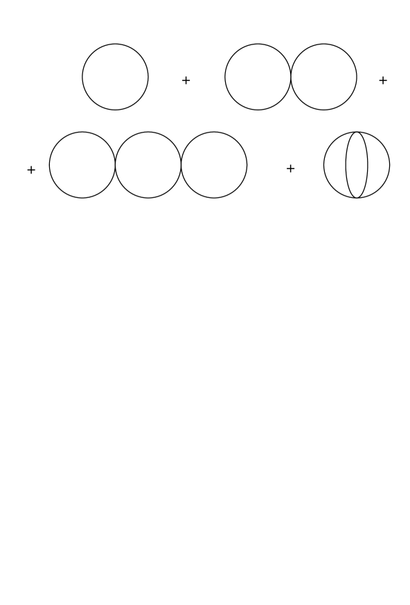
Figure 1: Vacuum diagrams contributing to the free energy density in a scalar theory.

An attempt to compute perturbatively the statistical sum or Green’s functions at sufficiently large temperatures immediately shows the trouble $\!{}^{{\bf?}}$. As the simplest example let us take the theory (8) and compute its statistical sum. In perturbation theory, it is given by a set of vacuum graphs, see Fig. 1. Consider the temperatures $T\gg m$. Then, with the use of Feynman rules defined above, it is easy to see that in addition to an ordinary, zero-temperature expansion parameter, $\sim\lambda$, a new expansion parameter appears,

$$\sim\frac{\lambda T}{m}.$$ (9)

A most simple way to see this is to take the $n=0$ contribution to the statistical sum (as we will see later, these modes are crucial in constructing effective field theories). The simple loop gives $m^{3}T$, the “figure of eight” graph gives $\lambda T^{2}m^{2}$, etc. Therefore, the straightforward perturbation theory breaks down at $T>m/\lambda$. For the theories containing, in perturbation theory, massless bosons (such as QCD) perturbation theory does not work for any temperature $\!{}^{{\bf?},{\bf?}}$.

There is a deep physical reason why this happens. At zero temperature we apply perturbation theory for consideration of processes where only a small number of particles participate. Thus, the expansion parameter is $\lambda$. At high temperatures, the number of particles, participating in collisions, may be large. Moreover, for bosonic degrees of freedom there is a well-known Bose amplification factor, associated with the bosonic distribution

$$n_{B}(E)=\frac{1}{\exp(E/T)-1},$$ (10)

where $E=\sqrt{k^{2}+m^{2}}$ is the particle energy. So, the expansion parameter becomes $\lambda n(E)$, coinciding with (9) at small momenta.

In fact, perturbation theory breaks down in the most interesting place, namely at the temperatures where different phase transitions are expected. One of the ways to deal with this problem is to rearrange the perturbative series and make a resummation of the most divergent diagrams. Partially, this helps in some cases. For example, for our pure scalar model the summation of the bubble graphs is equivalent to the introduction of the temperature-dependent scalar mass, which comes from one-loop corrections $\!{}^{{\bf?}}$ (see fig. 2):

$$m_{eff}^{2}(T)=m^{2}+\frac{\lambda}{4}T^{2},$$ (11)

which is to be used in propagators. For positive $m^{2}$ this procedure saves the situation and allows the perturbative computation of all properties of the equilibrium plasma in this theory. An interesting thing is that at high temperatures the expansion parameter of the resummed perturbation theory is $\frac{\lambda T}{m_{eff}}\sim\sqrt{\lambda}$ rather than $\lambda$. For negative values of $m^{2}$, corresponding to the spontaneous symmetry breaking at zero temperatures, even resummed perturbation theory breaks down near the point $m_{eff}^{2}(T)\simeq 0$, failing do describe the details of the symmetry-restoring phase transition which occurs there.

Figure 2: One-loop correction to the scalar mass.

Take now realistic theories. The resummed perturbation theory does not solve the problem, say, in QCD. The static gluon ($n=0$ component of the gauge field) mass remains zero in the one-loop approximation, so that infrared divergence inherent in (9) is not cut. A typical energy scale $E$, at which this happens is $E\sim\alpha_{s}T$ $\!{}^{{\bf?},{\bf?}}$ and is much smaller than the temperature itself because, according to our assumption, the coupling constants are small at the temperature under consideration. The same problem appears in the description of the phase transitions in gauge theories with scalars (such as EW theory and GUTs), where the gauge fields at high temperature are massless in perturbation theory.

To summarize this discussion, even the resummed perturbation theory breaks down at some infrared energy scale $E_{infrared}\sim\alpha T$, where $\alpha$ is a typical coupling constant of the theory under consideration. Thus, a number of properties in high-temperature plasma and different phenomena such as phase transitions cannot be described by perturbation theory.

If perturbation theory breaks down a natural inclination would be the use of direct numerical non-perturbative methods, such as lattice Monte Carlo simulations. This approach does not work, however, for theories containing chiral fermions, since we do not know how to put these on the lattice. Thus, theories such as the EW theory or grand unified models cannot be studied on the lattice with their complete particle content. This problem does not appear in pure bosonic models or in theories containing vector-like fermions, such as QCD. These models can be simulated on the lattice, but computations are often very demanding. Quite ironically, the computations are more time consuming for weaker coupling constants. This can be seen as follows. At high temperatures, the average distance between particles is of the order of $T^{-1}$, and it is clear that the lattice spacing $a$ must be much smaller than this distance, $a\ll T^{-1}$. At the same time, the lattice size $Na$, where $N$ is the number of lattice sites in the spatial direction, must be much larger than the infrared scale, described above, i.e. $Na\gg(\alpha T)^{-1}$. Therefore, the lattice size is required to be rather large, $N\gg\frac{1}{\alpha}$, the larger the smaller the coupling constant is.

The next section describes the formalism which allows one to deal with these problems, at least when the effective coupling constants are small at the temperature under consideration. Other limitations of the effective field theory approach will be considered later.

5 Effective field theory approach

The main idea of the effective theory approach to high-temperature field theory is the factorization of weakly coupled high-momentum modes, with energy $E\gg\alpha T$, and of strongly coupled infrared modes with energy $E<\alpha T$, and the construction of an effective theory for infrared modes only. The construction of the effective field theory is perturbative, while its analysis may be non-perturbative. Different methods can be applied: $\epsilon$ expansion, exact renormalization group, gap equations, Monte Carlo simulations, etc. Thus, a combination of perturbative and non-perturbative methods is to be used to solve the problem. The idea of this construction, known as dimensional reduction, goes back to the papers by Ginsparg $\!{}^{{\bf?}}$, and by Appelquist and Pisarski $\!{}^{{\bf?}}$. It was developed in refs. $\!{}^{{\bf?},{\bf?},{\bf?},{\bf?}}$, in application to the phase transitions and applied to hot QCD in refs. $\!{}^{{\bf?},{\bf?},{\bf?},{\bf?},{\bf?}}$. Different aspects of dimensional reduction were studied in refs. $\!{}^{{\bf?},{\bf?},{\bf?}}$.

The Euclidean formulation of the finite temperature field theory, described in section 2, provides a natural recipe for the construction of effective field theory. We learned there that the finite-temperature equilibrium field theory is equivalent to the Euclidean field theory defined on a finite time interval. Let us expand the bosonic and fermionic fields into Fourier sums,

$$\phi(x,\tau)=\sum_{n=-\infty}^{\infty}\phi_{n}(x)\exp(i\omega^{b}_{n}\tau),$$ (12)

$$\psi(x,\tau)=\sum_{n=-\infty}^{\infty}\psi_{n}(x)\exp(i\omega^{f}_{n}\tau),$$ (13)

where $\omega^{b}_{n}=2n\pi T$ and $\omega^{f}_{n}=(2n+1)\pi T$. After inserting these expressions into the action, the integration over time can be performed explicitly. As a result, we get a three-dimensional action, containing an infinite number of fields, corresponding to different Matsubara frequencies. Symbolically,

$$\int d^{4}xL\rightarrow\sum\int d^{3}xL^{3d}.$$ (14)

Therefore, a 4d finite-temperature field theory is equivalent to a 3d theory with an infinite number of fields, and 3d boson and fermion masses are just the frequencies $\omega^{b}$ and $\omega^{f}$. One can easily recognize here a perfect analogy to Kaluza–Klein theories with compact higher-dimensional space coordinates.

Now comes a crucial step. The 3d “superheavy” modes (fields with masses $\sim\pi T$) interact weakly with each other and with light modes (bosonic fields corresponding to the zero Matsubara frequency). Therefore, they can be “integrated out” with the use of perturbation theory, so that the 3d effective action, containing zero modes of bosonic fields, can be constructed. Formally,

$$\exp(-S_{eff})=\int D\Psi D\phi_{n}\exp(-S_{E}),$$ (15)

where the product is taken over non-zero frequencies. The effective action contains the bosonic fields only and can be written in the form

$$S_{eff}=cVT^{3}+\int d^{3}x\left[L_{b}(T)+\sum_{n=0}^{\infty}\frac{O_{n}}{T^{n}}\right],$$ (16)

where $L_{b}(T)$ is a super-renormalizable 3d effective bosonic Lagrangian with temperature-dependent constants, containing a scalar self-interaction up to the fourth power, $O_{n}$ are operators of dimensionality $n+3$, suppressed by powers of temperature at $n\geq 1$, $c$ is a perturbatively computable number (contribution of $n\neq 0$ modes to the free energy density). The existence of the effective action is closely related to the decoupling theorem $\!{}^{{\bf?},{\bf?}}$.

A way to compute the effective action of the theory is by a matching procedure, which has a lot in common with the corresponding method for heavy quarks, described at this school by M. Neubert. Write the most general 3d effective action, containing the light bosonic fields only, and fix its parameters (coupling constants and counterterms) by requiring that 3d Green’s functions at small spatial momenta $k\ll T$, computed with an effective Lagrangian, coincide with the initial 4d static Green’s functions up to some accuracy,

$$G^{3d}(k_{1},...k_{n})=G^{4d}_{\omega=0}(k_{1},...k_{n})(1+O(g^{m})).$$ (17)

Depending on the level of required accuracy, different numbers of operators $O_{n}$ must be included in the effective theory. For a generic gauge theory with $\lambda\sim g^{2},f\sim g$, where $\lambda$ ($f$) is a typical scalar self-coupling (fermion Yukawa coupling), $m=4$ for a super-renormalizable part of the effective theory, i.e. when all operators $O_{n}$ are dropped.

The following, evident consistency check must be applied to the constructed effective field theory. The typical energy scales (masses of excitations in 3d theory $m_{eff}$) must be small compared with the energy scale $\pi T$ that we have integrated out:

$$\left(\frac{m_{eff}}{\pi T}\right)^{2}\ll 1.$$ (18)

In fact, the 3d approximation generalizes the so-called high-temperature expansion often applied to the construction of the effective potential of the scalar field at high temperatures.

After the effective field theory is constructed, the statistical sum is expressed through the functional integral over 3d bosonic fields only:

$$Z=\int D\phi(x)\exp(-S_{eff}).$$ (19)

In some cases this integral can be computed with the help of the perturbation theory, but in general its evaluation requires different non-perturbative methods.

The construction, described above, looks quite formal. Nevertheless, it has a nice physical interpretation associated with the classical statistics of the field theory. Indeed, consider the bosonic fields appearing in $L_{b}(T)$ as generalized coordinates for some classical field theory with the Hamiltonian

$$H=\int d^{3}x~{}\left[\frac{1}{2}\sum P_{i}(x)^{2}+TL_{b}(T)\right],$$ (20)

where $P_{i}(x)$ is a set of generalized momenta. Now, the partition function for this classical system is given by the functional integral

$$Z=\int DP(x)D\phi(x)\exp\left(-\frac{H}{T}\right),$$ (21)

which coincides with eq. (19) after the integration over momenta. Thus, it is often said that the high-temperature limit of the quantum field theory is given by the classical statistics $\!{}^{{\bf?}}$.

We will demonstrate how this general procedure works on specific examples in the next section. As we will see, in several cases further simplification of the effective theory is possible.

6 Examples

6.1 Pure scalar field theory

Let us first consider a simplest scalar theory with the 4d Lagrangian defined by eq. (8). According to our rules, we must write down the most general 3d Lagrangian, consistent with the symmetries of the theory. It looks like:

$$L_{eff}=\frac{1}{2}(\partial_{i}\phi_{3})^{2}+\frac{1}{2}m_{3}^{2}\phi_{3}^{2}+\frac{1}{4}\lambda_{3}\phi_{3}^{4}+\Delta L,$$ (22)

where $\Delta L$ represents the contribution of higher-order operators. In 3d, the dimensionality of the different coupling constants and scalar field are: $\phi_{3}$: GeV${}^{\frac{1}{2}}$; $m_{3}^{2}$ : GeV²; $\lambda_{3}$: GeV. The mapping procedure on the tree level (sometimes called naive dimensional reduction) immediately gives the relation of 3d field to 4d field: $\phi_{3}=\phi/\sqrt{T}$, and other 3d parameters are given by $m_{3}^{2}=m^{2}$ and $\lambda_{3}=\lambda T$.

The structure of one-loop corrections to these relations can be easily found on general grounds. An important fact is that the 3d theory is super-renorma-lizable and contains a finite number of divergent diagrams only. The ultraviolet renormalization of the coupling $\lambda_{3}$ is absent in any order of perturbation theory, while the mass term contains linear and logarithmic divergences on the one- and two-loop levels respectively. At the same time, the 4d self-coupling $\lambda$ and mass $m$ are scale-dependent. Thus, on the one-loop level the relation of the 3d parameters to the 4d ones must have the form:

$$m_{3}^{2}=m^{2}(\mu)\left[1+\beta_{m}\log\frac{\mu_{T}}{\mu}\right]+A\lambda T^{2},$$

$$\lambda_{3}=\lambda(\mu)T\left[1+\beta_{\lambda}\log\frac{\mu_{T}}{\mu}\right],$$ (23)

where $\beta_{m}$ and $\beta_{\lambda}$ are the $\beta$-functions corresponding to the running mass and self-coupling. The parameters $A$ and $\mu_{T}$ cannot be fixed by the requirement of renormalization group invariance and are to be found by explicit computation of diagrams in Figs. 2 and 3. In the modified minimal subtraction scheme ${\overline{{\rm MS}}}$ they are:

$$\mu_{T}=4\pi Te^{-\gamma}\approx 7T,~{}~{}~{}A=\frac{1}{4}.$$ (24)

In eqs. (23) the parameter $\mu$ is arbitrary, and taking it to be $\mu=\mu_{T}$ minimizes the corrections. This allows us to rewrite these equations in a simpler form, $\lambda_{3}=\lambda(\mu_{T})T$, $m_{3}^{2}=\frac{1}{4}\lambda(\mu_{T})T^{2}+m^{2}(\mu_{T})$. The appearance of the running mass and 4d coupling constant at scale $\sim T$ clarifies our requirement concerning the amplitude of the coupling constant, needed for the perturbative construction of the effective field theory. The higher-order corrections to relations (23) can also be found.

Figure 3: One loop correction to the coupling constant.

The super-renormalizable theory gives the accuracy in Green’s function $\frac{\Delta G}{G}\sim O(\lambda^{2})$ provided we have spatial momenta $k\ll T$ and a 3d mass $|m_{3}^{2}|\ll T^{2}$. A further increase in the accuracy may be achieved by adding higher-order operators. The one with dimensionality three appears on the one-loop level and is equal to $h\phi_{3}^{6}$, with

$$h=\frac{9\zeta(3)}{256\pi^{4}}\lambda^{3}.$$

Just on dimensional grounds, the perturbative expansion parameter in the effective 3d theory is $\lambda_{3}/m_{3}$. Thus, if the spontaneous symmetry breaking is absent at zero temperature ($m^{2}>0$), then the 3d theory is weakly coupled in the whole range of temperatures (of course, below the Landau pole). Thus, all equilibrium properties of a high-temperature state can be computed by first constructing the effective field theory and then by perturbative computations in the effective theory. In the opposite case, when $m^{2}$ is negative, the symmetry $\phi\rightarrow-\phi$ is broken at zero temperature, and the scalar field acquires a non-zero vacuum expectation value:

$$v^{2}=-\frac{m^{2}}{\lambda}.$$ (25)

As seen from our effective Lagrangian (22), the 3d mass changes its sign at

$$T_{c}^{2}=-\frac{4m^{2}}{\lambda},~{}~{}~{}T_{c}=2v,$$ (26)

which is nothing but an estimate of the critical temperature of the phase transition with restoration of the $\phi\rightarrow-\phi$ symmetry. The mass squared of the particle excitation in the tree approximation is given by $m_{3}^{2}$ at $T>T_{c}$ and by $-2m_{3}^{2}$ at $T<T_{c}$. The perturbative analysis of the effective theory near $T=T_{c}$ breaks down, since the expansion parameter $\lambda_{3}/|m_{3}|$ diverges near this point. Non-perturbative methods (such as $\epsilon$-expansion or lattice simulations) are needed in order to clarify the nature of the system here.

Let us consider the advantages we gain by the construction of the effective field theory. The straightforward perturbative analysis of the original theory is valid for $\lambda\ll 1$ and $T^{2}\ll\frac{|m^{2}|}{\lambda}$. The construction of the effective field theory requires only $\lambda\ll 1$ and $|m^{2}|\ll(\pi T)^{2}$. In particular, it is applicable near the temperature of the phase transition $T_{c}$. The original 4d theory at $T^{2}>\frac{m^{2}}{\lambda}$ contains at least two important energy scales: an ultraviolet one $\sim T$ and the infrared one $\sim m_{3}$; the effective theory contains an infrared scale only. Beyond the phase transition, the theory is perturbatively solvable, and the effective field theory approach provides a convenient recipe for resumming the perturbation theory.

6.2 QCD

The QCD Lagrangian for $n_{f}$ quark flavours is given by

$$L={1\over 4}F_{\mu\nu}F_{\mu\nu}+\sum\bar{\psi}_{i}(\gamma_{\nu}D_{\nu}-m_{i})\psi_{i}.$$ (27)

For simplicity, let us consider the limit $T\gg m_{i}$. The 3d effective Lagrangian contains gauge fields $A_{i}^{a}$ and a scalar octet $A_{0}^{a}$, $a=1,...,8$, where $A_{0}$ is a temporal component of the 4d gauge field. The most general super-renormalizable 3d Lagrangian, containing these fields, is

$$L_{3}={1\over 4}F_{ij}F_{ij}+\frac{1}{2}(D_{i}A_{0}^{a})^{2}+\frac{1}{2}m_{D}^{2}A_{0}^{a}A_{0}^{a}+\frac{1}{4}\lambda_{A}(A_{0}^{a}A_{0}^{a})^{2}.$$ (28)

Here $D_{i}$ is a covariant derivative in adjoint representation. Of course, on the tree level $m_{A}^{2}=0$ and $\lambda_{A}=0$ because of the structure of the 4d Lagrangian. The one-loop relations in the ${\overline{{\rm MS}}}$ scheme are $\!{}^{{\bf?},{\bf?},{\bf?}}$:

$$g_{3}^{2} = g^{2}(\mu)T\biggl{[}1+\frac{g^{2}}{16\pi^{2}}\biggl{(}11L_{b}-\frac{2n_{f}}{3}L_{f}+1\biggr{)}\biggr{]},$$ (29)

$$m_{D}^{2} = g^{2}(\mu)T^{2}\left(1+\frac{n_{f}}{6}\right),$$ (30)

$$\lambda_{A} = =\frac{3g^{4}(\mu)T}{8\pi^{2}}\left(1-\frac{n_{f}}{9}\right)$$ (31)

where

$$L_{b}=2\log\frac{\mu}{\mu_{T}},~{}~{}~{}L_{f}=2\log\frac{4\mu}{\mu_{T}}.$$ (32)

The logarithmic corrections to $m_{D}^{2}$ and $\lambda_{A}$ appear on two-loop level only. The non-zero value of $m_{D}$ (the Debye mass) ensures the screening of chromo-electric fields in a high-temperature plasma and the absence of confinement.

Because of asymptotic freedom, the effective theory is valid at sufficiently high temperatures, when $\alpha_{s}(\mu_{T})/\pi\ll 1$. In other words, it is applicable to the quark-gluon phase of QCD only and describes physics on the energy scales $k\ll T$, but $k$ may be as large as $gT$.

The 3d Lagrangian (28) contains two essential mass scales. The largest one is the Debye screening mass $\sim gT$, and the smallest scale is associated with the 3d gauge coupling constant $\alpha_{3}=\alpha_{s}T$. The scale hierarchy $\alpha_{3}\ll m_{D}$, appearing when the effective field theory approach is valid, suggests that a further simplification of the effective theory is possible. Namely, the “heavy” scale $\sim gT$ (we used the term “superheavy” for the scale $\sim T$) can be integrated out. The construction of the “second” level of effective field theory, containing the chromo-magnetic gauge fields only, goes precisely along the lines described above. The result is a pure SU(3) Yang–Mills theory, describing the interaction of soft modes with momenta $k\ll gT$, but $k$ may be as large as $g^{2}T$. The Lagrangian is:

$$L_{eff}={1\over 4}F_{ij}F_{ij}.$$ (33)

In the one-loop approximation the new gauge coupling is $\!{}^{{\bf?}}$:

$$\bar{g}_{3}^{2}=g_{3}^{2}\left(1-\frac{g_{3}^{2}}{16\pi m_{D}}\right),$$ (34)

and the accuracy of an effective description by a pure gauge theory at momenta $k\ll gT$ is $\frac{\Delta G}{G}\sim O(g^{3})$ $\!{}^{{\bf?}}$.

The 3d pure gauge theory which appeared as a final stage of dimensional reduction contains just one scale, $\alpha_{3}$. It is strongly coupled at small energies and is believed to be confining. No perturbative methods are available for its study. Thus, high-temperature QCD, in spite of asymptotic freedom, contains a piece of non-perturbative physics described by a pure Yang–Mills theory in 3d. A simple power counting allows one to find easily the limits of perturbation theory for the study of high-temperature QCD. Let us take, for example, free energy. From dimensional grounds, the contribution from the non-perturbative pure 3d sector is of the order of $\alpha_{3}^{3}T$. Thus, the $O(g^{6})T^{4}$ correction to the free energy cannot be computed perturbatively. Recently, the perturbative computations were pushed to the very end: the $O(g^{4})$ corrections to the free energy were computed in refs. $\!{}^{{\bf?},{\bf?}}$ and $O(g^{5})$ in $\!{}^{{\bf?},{\bf?},{\bf?}}$. In order to find the $O(g^{6})$ contribution, a non-perturbative method, such as lattice Monte Carlo simulations, must be applied to solve the pure 3d model. In addition, a number of 4-loop computations should be done.

6.3 Electroweak theory

Our experience with the pure scalar theory and QCD allows us an easy guess of the effective 3d action for soft strongly interacting bosonic modes with $k\ll gT$, describing the high-temperature EW theory. This is just the 3d SU(2)$\times$ U(1) gauge theory with the doublet of scalar fields with the Lagrangian

$$L=\frac{1}{4}G^{a}_{ij}G^{a}_{ij}+\frac{1}{4}F_{ij}F_{ij}+(D_{i}\Phi)^{\dagger}(D_{i}\Phi)+\bar{m}_{3}^{2}\Phi^{\dagger}\Phi+\bar{\lambda}_{3}(\Phi^{\dagger}\Phi)^{2},$$ (35)

where $G_{ij}^{a}$ and $F_{ij}$ are the SU(2) and U(1) field strengths, respectively, $\Phi$ is a scalar doublet, and $D_{i}$ is a standard covariant derivative in the fundamental representation. The four parameters of the 3d theory (scalar mass $\bar{m}_{3}^{2}$, scalar self-coupling constant $\bar{\lambda}_{3}$, and two gauge couplings $\bar{g}_{3}$ and $\bar{g}^{\prime}_{3}$) are some functions of the initial parameters and temperature. They were computed in the one- and partially in the two-loop approximation in refs. $\!{}^{{\bf?},{\bf?}}$; we present here just the tree relations for the coupling constants:

$$g_{3}^{2}=g^{2}T,~{}~{}~{}g_{3}^{\prime 2}=g^{\prime 2}T,~{}~{}~{}\lambda_{3}=\lambda T,$$ (36)

and the one-loop relation for the scalar mass:

$$m_{3}^{2}(\mu)=-\frac{1}{2}m_{H}^{2}+T^{2}\biggl{(}\frac{1}{2}\lambda+\frac{3}{16}g^{2}+\frac{1}{16}g^{\prime 2}+\frac{1}{4}g_{Y}^{2}\biggr{)}.$$ (37)

Here $m_{H}$ is the zero-temperature Higgs mass, $g_{Y}$ is the Yukawa coupling constant corresponding to the $t$-quark.

As usual, the effective action does not contain fermions since their 3d masses are “superheavy”. It does not contain zero components of the gauge fields – triplet and singlet of SU(2) – because these are “heavy” according to our classification of scales.

The most interesting area of application of the effective action (35) is the region of temperatures where the electroweak phase transition is expected to occur. As in the case of the pure scalar theory, a rough estimate of the critical temperature follows from the requirement that the 3d mass of the scalar field is close to zero, $\bar{m}_{3}^{2}=0$. In the vicinity of this point the effective Lagrangian (35) has a much wider area of application than the minimal Standard Model (MSM). In fact, it plays the role of the universal theory which describes the phase transition in a number of extensions of the Standard Model at least in a part of their parameter space. The set of models includes the minimal supersymmetric Standard Model (MSSM) and some extended versions of it, an electroweak theory with two scalar doublets, etc. One may wonder where are the other scalars, typical for the extensions of the Standard Model. The answer is that all extra scalar degrees of freedom are naturally “heavy” (mass $\sim gT$) near the phase transition temperature and can be integrated out.

Indeed, let us take as an example the two-Higgs doublet model. The integration over the “superheavy” modes gives a 3d SU(2)$\times$U(1) theory with an extra Higgs doublet in addition to the theory considered above. Construct now the one-loop scalar mass matrix for the doublets and find the temperatures at which one of its eigenvalues is zero. Take the higher temperature; this is the temperature near which the phase transition takes place. Determine the mass of the other scalar at this temperature. Generally, it is of the order of $gT$, and therefore, it is heavy. Integrate this heavy scalar out – the result is eq. (35). In the case when both scalars are light near the critical temperature, a more complicated model, containing two scalar doublets, should be studied. It is clear, however, that this case requires fine tuning.

The same strategy is applicable to the MSSM. If there is no breaking of colour and charge at high temperature (breaking is possible, in principle, since the theory contains squarks), then all degrees of freedom, excluding those belonging to the two-Higgs doublet model, can be integrated out. We then return back to the case considered previously. The conclusion in this case is similar to the previous one, namely that the phase transition in the MSSM can be described by a 3d SU(2)$\times$U(1) gauge–Higgs model, at least in a considerable part of the parameter space. The explicit relations were worked out in refs. $\!{}^{{\bf?},{\bf?},{\bf?}}$. What changes from going from one theory to another is the explicit perturbative relations between initial 4d parameters and parameters of the effective theory; if two different 4d theories have the same 3d couplings, the electroweak phase transition occurs in them in a similar way. The effective field theory approach again demonstrates its strength: instead of studying many models with different particle content, it is sufficient to study just one 3d effective theory by non-perturbative means; the result of this study may be used for many 4d models after perturbative computations of 4d $\rightarrow$ 3d mapping.

7 Electroweak phase transition

One of the most interesting areas of application of finite-temperature field theory are phase transitions. Our interest in this section will be an EW theory. The strength of the electroweak phase transition is important for a number of cosmological applications. For example, all mechanisms of electroweak baryogenesis require that the phase transition should be strong enough, i.e. $\!{}^{{\bf?},{\bf?}}$

$$v(T_{c})/T_{c}>1,$$ (38)

where $v(T_{c})$ is the vacuum expectation value of the Higgs field at the critical temperature.

As we have learned in the previous section, to study the electroweak phase transition it is sufficient to study an SU(2)$\times$U(1) gauge–Higgs theory in 3d. Let us simplify even further and omit the U(1) factor. Numerically the U(1) coupling constant $g^{\prime}$ is smaller than the SU(2) one $g$; thus the corrections are expected to be small. In this case, the Lagrangian is

$$L=\frac{1}{4}G^{a}_{ij}G^{a}_{ij}+(D_{i}\Phi)^{\dagger}(D_{i}\Phi)+\bar{m}_{3}^{2}\Phi^{\dagger}\Phi+\bar{\lambda}_{3}(\Phi^{\dagger}\Phi)^{2}.$$ (39)

This 3d theory is defined by one dimensionful parameter $g_{3}^{2}\sim g^{2}T$ and two dimensionless ratios

$$\qquad x\equiv{\bar{\lambda}_{3}\over\bar{g}_{3}^{2}},\qquad y\equiv\frac{\bar{m}_{3}^{2}}{\bar{g}_{3}^{4}}.$$ (40)

The dimensionful coupling constant can be chosen to fix the energy scale. Therefore, the phase state of this theory is completely defined by the two numbers $x$ and $y$. For the MSM the dependence of the parameter $x$ on the mass of the Higgs boson near the critical temperature (near $y=0$) is shown in Fig. 4.

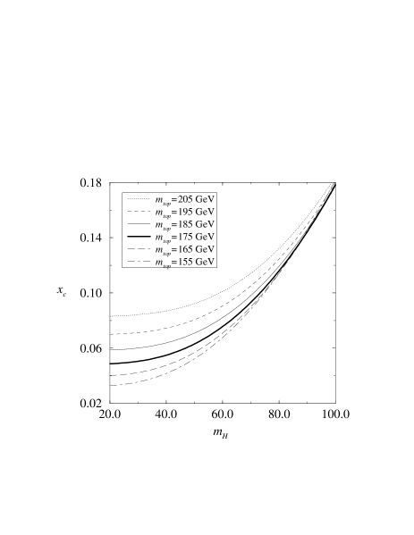
Figure 4: The value $x=\lambda_{3}/g_{3}^{2}$ as a function of the physical Higgs mass $m_{H}$ and the top quark mass $m_{\rm top}$ near the critical temperature defined from taking $m_{3}^{2}=0$. In general, $x$ depends on the Higgs mass, the top mass, and logarithmically on the temperature. From ref. $\!{}^{{\bf?}}$.

At first glance there are two phases in this theory. When the Higgs mass is positive, $y>0$, one would say that this theory is analogous to QCD with scalar quarks. Thus, we are in the “confinement” phase (other names of this phase are “symmetric” or “restored” phase) and the particle spectrum consists of the bound states of the scalar quarks, such as

$$\pi=\Phi^{\dagger}\Phi,\quad W_{j}^{0}=i(\Phi^{\dagger}D_{j}\Phi-(D_{j}\Phi)^{\dagger}\Phi),$$

$$W_{j}^{+}=(W_{j}^{-})^{*}=(\Phi^{\dagger}D_{j}{\tilde{\Phi}}-(D_{j}\Phi)^{\dagger}{\tilde{\Phi}}).$$ (41)

Here $\tilde{\Phi}=i\tau_{2}\Phi^{*}$.

On the contrary, if the scalar mass is negative, one would say that the SU(2) gauge symmetry is broken, and the initially massless gauge bosons acquire non-zero masses. This phase is usually called “broken” or Higgs. In the usual folklore, the particle spectrum consists of fundamental massive gauge bosons and the Higgs particle.

When the temperature changes, the sign of the effective mass term changes. If the consideration presented above were true, one would expect to have a first-order or second-order phase transition between the two phases. In fact, the gauge symmetry is never “broken” – all physical observables by construction are gauge-invariant. Moreover, there is no gauge-invariant local order-parameter that can distinguish between the “broken” (Higgs) and “restored” (symmetric or confinement) phases $\!{}^{{\bf?},{\bf?}}$. The bound states defined in (41) are complementary to the “elementary” excitations in the Higgs phase. A simple exercise shows that in the Higgs phase in unitary gauge the composite fields defined by eq. (41) are proportional to the “elementary” fields corresponding to the Higgs particle and vector bosons. Thus, in a strict sense, there is no gauge symmetry restoration at high temperatures, but there can be (but not necessarily are) phase transitions.

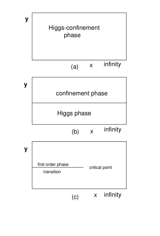
Figure 5: Three possible types of phase diagram for the SU(2) gauge–Higgs system.

This general consideration suggests three possible phase diagrams for the SU(2)–Higgs model (Fig. 5). First, because the qualitative difference between symmetric and Higgs phases is absent, we can have only one phase (Higgs-confinement phase) everywhere at the $(x,y)$ plane (Fig. 5a). Of course, different points at this plane correspond to the theories which are quantitatively different; nevertheless one theory can be analytically transformed to another one. In the latter case any high-temperature phase transition is absent. Another possibility is that there is a first-order transition line separating the “symmetric” phase from the “broken” phase. In this case the first-order phase transition occurs at any value of the scalar self-coupling constant (Fig. 5b). An intermediate possibility is when a first order phase transition line has an end-point somewhere on the phase plane (Fig. 5c). Then at $x<x_{crit}$ the phase transition is of the first kind, at $x=x_{c}$ the phase transition is of the second kind, and at $x>x_{c}$ the phase transition is absent.

Of course, some computations are necessary in order to clarify the phase structure. A simple one-loop perturbative analysis allows Fig. 5a to be ruled out, but cannot distinguish between Fig. 5b and Fig. 5c.

Let us define the field-dependent vector boson mass as

$$m_{T}=\frac{1}{2}g_{3}\phi,$$ (42)

and scalar masses as

$$m_{1}^{2}=m_{3}^{2}+3\lambda_{3}\phi^{2},$$ (43)

$$m_{2}^{2}=m_{3}^{2}+\lambda_{3}\phi^{2}.$$

Then the 1-loop effective potential for the scalar field is

$$V_{1}(\phi)=\frac{1}{2}m_{3}^{2}\phi^{2}+\frac{1}{4}\lambda_{3}\phi^{4}-{1\over 12\pi}\biggl{(}6m_{T}^{3}+m_{1}^{3}+3m_{2}^{3}\biggr{)}.$$ (44)

This effective potential describes a first-order phase transition, since at the critical value of $m_{3}^{2}$ the jump of the order parameter $\phi$ is non-zero. Is the conclusion about the first-order nature of the phase transition reliable? To answer this question, one can estimate the value of the field $\phi$ at the maximum of the effective potential. At sufficiently small values of $\lambda_{3}$ it is of the order of $\phi_{max}\sim\frac{g_{3}^{3}}{\pi\lambda_{3}}$. The dimensionless expansion parameter at this point is $\frac{g_{3}^{2}}{\pi m_{T}}\sim\frac{\lambda_{3}}{g_{3}^{2}}=x$. Thus, the existence of the maximum of the effective potential is reliable at small values of $x$ (small Higgs masses in zero-temperature language). Therefore, the “symmetric” and the “broken” phases are separated by a first-order phase transition line, at least at small $x$. At larger $x$ perturbation theory is not to be trusted, and the nature of the phase transition can be clarified only by some kind of non-perturbative analysis. An argument in favour of Fig. 5b follows from the $\epsilon$-expansion $\!{}^{{\bf?},{\bf?}}$ while an indication that the scenario of Fig. 5c may be realized comes from the study of 1-loop gap equations $\!{}^{{\bf?}}$.

The 3d lattice MC simulations, done in $\!{}^{{\bf?}}$, have established the absence of first-and second-order phase transitions at $x>0.18$ and singled out the phase diagram of the type shown in Fig. 5c. The value of the end-point of the first-order phase transition line is likely to be near $x={1\over 8}$, i.e. there is no phase transition at Higgs masses greater than $80$ GeV in the minimal Standard Model. In this case it is quite unlikely that there are any cosmological consequences coming from the EW epoch. The 4d lattice simulations at sufficiently small Higgs masses of a pure bosonic model were carried out in refs. $\!{}^{{\bf?},{\bf?},{\bf?},{\bf?},{\bf?}}$. Whenever the comparison between 3d and 4d simulations is possible, they are in agreement, indicating the correctness of the dimensional reduction beyond perturbation theory.

The requirement of the EW baryogenesis provides an even stronger constraint on the strength of the EW phase transition. In fact, the constraint (38) does not hold for any Higgs mass in the MSM (if the mass of the top quark is $175$ GeV) $\!{}^{{\bf?}}$. It is possible to satisfy this constraint in a specific portion of the parameter space of the MSSM $\!{}^{{\bf?}}$: the Higgs mass is smaller than the $Z$ mass, the lightest stop mass is smaller than the top mass, and $\tan\beta<3$. This prediction can be tested at LEP2.

Near the critical point (the end-point of the first-order phase transition line) the 3d gauge–Higgs system admits a further simplification at large distances $\gg\frac{1}{g_{3}^{2}}$. At the critical point the phase transition is of second order, thus there is a massless scalar particle. The effective theory describing this nearly massless state is a simple scalar theory of some field $\chi$ with the Lagrangian

$$L=\frac{1}{2}(\partial_{i}\chi)^{2}+\frac{1}{2}m^{2}\chi^{2}+\lambda_{\chi}\chi^{4}+h\chi.$$ (45)

It is a challenge to define a mapping of the parameters of the gauge SU(2) Higgs model to the parameters of the scalar theory, since the perturbative methods fail in the strong coupling limit.

8 Conclusion

The effective field theory approach is a powerful method for studying high-temperature equilibrium field theory. It has allowed to solve a number of long-standing problems of high-temperature gauge theories. The list includes the infrared problem of the thermodynamics of Yang–Mills fields and the problem of the EW phase transition. The method allows reliable computations of the properties of the high-temperature equilibrium plasma of elementary particles.

Of course, the method has a number of limitations. It cannot be used in theories where coupling constants are large at the scale of the order of the temperature. It does not work at temperatures below the relevant mass scales. It is not applicable to time-dependent phenomena and cannot be used for computation of transport coefficients such as viscosity, etc. However, it allows a description of the ground state of the system at high temperatures, therefore providing a starting point for the study of non-equilibrium phenomena.

I am grateful to Mikko Laine and Keijo Kajantie for reading of the manuscript and helpful comments.

References

References

- [1] Ya.B. Zeldovich and I. D. Novikov. Structure and Evolution of the Universe. Nauka, Moscow, 1975.
- [2] E.W. Kolb and M.S. Turner. The Early Universe. Addison-Wesley, Reading, MA, 1990.
- [3] D.A. Kirzhnitz. JETP Lett., 15:529, 1972.
- [4] D.A. Kirzhnitz and A.D. Linde. Phys. Lett., 72B:471, 1972.
- [5] L. Dolan and R. Jackiw. Phys. Rev., D9:3320, 1974.
- [6] S. Weinberg. Phys. Rev., D9:3357, 1974.
- [7] A.M. Polyakov. Phys. Lett., 72B:477, 1978.
- [8] L. Susskind. Phys. Rev., D20:2610, 1979.
- [9] K.J. Eskola, K. Kajantie, and J. Lindfors. Phys.Lett., B214:613, 1988.
- [10] J. Cleymans and H. Satz. Z. Phys, C57:135, 1993.
- [11] K. Geiger and B. Muller. Nucl. Phys., B369:600, 1992.
- [12] H. Satz. Z. Phys, C62:683, 1994.
- [13] D.A. Kirzhnits and A.D. Linde. Ann. Phys., 101:195, 1976.
- [14] A. Linde. Particle physics and inflationary cosmology. Chur, Switzerland: Harwood (Contemporary concepts in physics, 5), 1990.
- [15] J. Kapusta. Finite-Temperature Field Theory. Cambridge Monographs on Mathematical Physics, Cambridge University Press, 1989.
- [16] A.D. Linde. Phys. Lett., 96B:289, 1980.
- [17] D. Gross, R. Pisarski, and L. Yaffe. Rev. Mod. Phys., 53:43, 1981.
- [18] P. Ginsparg. Nucl. Phys., B170:388, 1980.
- [19] T. Appelquist and R. D. Pisarski. Phys. Rev., D23:2305, 1981.
- [20] K. Farakos, K. Kajantie, K. Rummukainen, and M. Shaposhnikov. Nucl. Phys., B425:67, 1994.
- [21] K. Farakos, K. Kajantie, K. Rummukainen, and M. Shaposhnikov. Nucl. Phys., B442:317, 1995.
- [22] K. Kajantie, M. Laine, K. Rummukainen, and M. Shaposhnikov. Nucl. Phys., B458:90, 1996.
- [23] K. Kajantie, M. Laine, K. Rummukainen, and M. Shaposhnikov. Nucl. Phys., B466:189, 1996.
- [24] E. Braaten and A. Nieto. Phys. Rev. Lett., 73:2402, 1994.
- [25] E. Braaten and A. Nieto. Phys. Rev., D51:6990, 1995.
- [26] E. Braaten. Phys. Rev. Lett., 74:2164, 1995.
- [27] E. Braaten and A. Nieto. Phys. Rev., D53:3421, 1996.
- [28] E. Braaten and A. Nieto. Phys. Rev. Lett., 76:1417, 1996.
- [29] R. Jackiw and S. Templeton. Phys. Rev., D23:2291, 1981.
- [30] N.P. Landsman. Nucl. Phys., B322:498, 1989.
- [31] A. Jakovac, K. Kajantie, and A. Patkos. Phys. Rev., D49:6810, 1994.
- [32] T. Appelquist and J. Carazzone. Phys. Rev., D11:2856, 1975.
- [33] S. Weinberg. Phys. Lett., 91B:51, 1980.
- [34] S.-Z. Huang and M. Lissia. Nucl. Phys., B438:54, 1995.
- [35] K. Farakos, K. Kajantie, K. Rummukainen, and M. Shaposhnikov. Phys. Lett., B336:494, 1994.
- [36] P. Arnold and C.-X. Zhai. Phys. Rev., D50:7603, 1994.
- [37] P. Arnold and C.-X. Zhai. Phys. Rev., D51:1906, 1995.
- [38] C.-X. Zhai and B. Kastening. hep-ph/9507380, 1995.
- [39] J.M. Cline and K. Kainulainen. hep-ph/9605235, 1996.
- [40] M. Losada. hep-ph/9605266, 1996.
- [41] M. Laine. hep-ph/9605283, 1996.
- [42] M. E. Shaposhnikov. JETP Lett., 44:465, 1986.
- [43] M. E. Shaposhnikov. Nucl. Phys., B287:757, 1987.
- [44] T. Banks and E. Rabinovici. Nucl. Phys., B160:349, 1979.
- [45] E. Fradkin and S.H. Shenker. Phys. Rev., D19:3682, 1979.
- [46] P. Arnold and L. G. Yaffe. Phys. Rev., D49:3003, 1994.
- [47] W. Buchmüller and O. Philipsen. Nucl. Phys., B443:47, 1995.
- [48] K. Kajantie, M. Laine, K. Rummukainen, and M. Shaposhnikov. hep-ph/9605288, 1996.
- [49] B. Bunk, E.M. Ilgenfritz, J. Kripfganz, and A. Schiller. Phys. Lett., B284:371, 1992.
- [50] B. Bunk, E.M. Ilgenfritz, J. Kripfganz, and A. Schiller. Nucl. Phys., B403:453, 1993.
- [51] Z. Fodor, J. Hein, K. Jansen, A. Jaster, and I. Montvay. Phys. Lett., B334:405, 1994.
- [52] Z. Fodor, J. Hein, K. Jansen, A. Jaster, and I. Montvay. Nucl. Phys., B439:147, 1995.
- [53] F. Csikor, Z. Fodor, J. Hein, and J. Heitger. Phys. Lett., B357:156, 1995.
- [54] M. Carena, M. Quiros, and C.E.M. Wagner. Phys. Lett., B380:81, 1996.