The Static Quark-Antiquark Potential in QCD to Three Loops

Abstract

The static potential between an infinitely heavy quark and antiquark is derived in the framework of perturbative QCD to three loops by performing a full calculation of the two-loop diagrams and using the renormalization group. The contribution of massless fermions is included.

TTP 96-37
October 1996
hep-ph/9610209

The force law between infinitely heavy quarks has been investigated since more than 20 years because of its importance for a deeper understanding of the strong interactions. The static quark-antiquark potential is a very fundamental concept, constituting the non-abelian analog to the Coulomb potential of electrodynamics, and also enters as a vital ingredient in the description of non-relativistic bound states like quarkonia. It is widely believed to consist of two parts: a Coulombic term at short distances which can be derived from field theory by using perturbative QCD, and a long-ranged confining term whose derivation from first principles presumably requires much more advanced methods. Although an analysis based on perturbation theory alone thus cannot give the complete potential, the result of such an effort would nevertheless be very useful. It could provide an improved input for QCD inspired potential models or even describe very heavy systems to a reasonable accuracy by itself. It could be compared with the potential obtained from numerical studies using lattice gauge theory and it might also give some hints on the nonperturbative regime.

The first investigation of the static perturbative QCD potential has been performed in [1]. Although this work has been extended by several groups shortly after [2, 3, 4, 5], and some of these also studied aspects of the two- [2] and even three-loop diagrams [4], there is still no full calculation of the two-loop diagrams available. The purpose of the present paper is to fill this gap and hence, by exploiting the renormalization group equation, to obtain the three-loop potential.

Before turning to the actual analysis, let us first recall the calculational procedure employed. It seems appropriate to begin with the simplest case, the Abelian theory without massless fermions.

The static potential in QED can be defined in a way which makes its gauge invariance manifest via the vacuum expectation value of a Wilson loop taken about a rectangle of width $R$ and length $T\gg R$:

$$V(R)=-\lim_{T\to\infty}\frac{1}{iT}\ln\langle P\exp\Big{(}ie\oint dx_{\mu}A^{\mu}\Big{)}\rangle$$ (1)

where $P$ denotes the path ordering prescription.

The functional integral can be calculated exactly, and one indeed finds the Coulomb potential plus an additional term which represents the self-energy of the sources [2]. To compare with the non-Abelian theory it is, however, useful to go through the perturbative analysis as well. The Feynman rules for the source are as follows: a source-photon vertex corresponds to a factor $iev^{\mu}$, with an additional minus sign for the “anti-source”, and the source “propagator” reads

$$S_{F}(x-x^{\prime})=-i\Theta(x_{0}-x_{0}^{\prime})\delta({\bf x}-{\bf x}^{\prime})$$ (2)

in coordinate space or

$$S_{F}(p)=\frac{1}{vp+i\varepsilon}$$ (3)

in momentum space. The four vector $v$ is given by $v^{\mu}=(1,{\bf 0})$ and has only been introduced for notational reasons. The appearance of a propagator for the sources is a consequence of the time ordering prescription in the path integral, which introduces $\Theta$-functions when expanding the exponential.

Looking at the problem in this way shows the connection to another approach: the potential beyond the infinite mass limit or for non-singlet sources is frequently also derived from the scattering operator; see for example [6, 7]. The static QED potential thus should be derivable from the scattering operator of heavy electron effective theory, the QED analog of heavy quark effective theory, and the Feynman rules given above obviously support this point of view.

Some care is required because the Feynman diagrams do not directly correspond to the potential but to $\exp[-iV(R)T]$. The consequence is that in the abelian theory the one-photon exchange amplitude already gives the final result:

$$-ie^{2}\int\!dx_{0}dy_{0}\;v_{\mu}v_{\nu}D^{\mu\nu}(x-y)=-ie^{2}T\int\!\frac{d^{3}q}{(2\pi)^{3}}\frac{e^{i{\bf qR}}}{-{\bf q}^{2}}$$

where $D^{\mu\nu}$ is used to represent the photon propagator and ${\bf x}=0$, ${\bf y}={\bf R}$ are understood.

Figure 1: One-loop ladder diagrams. The double lines indicate static sources.

At one loop order, one encounters self-energy and vertex corrections which cancel due to the Ward identity, and the ladder diagrams shown in Fig. 1 which are best analyzed in coordinate space. Because of the simple structure of the source propagator, Eq. (2), only integrations over time-variables remain. Adding the two diagrams removes the $\Theta$-function corresponding to the anti-source propagator, and adding them once more with $x\leftrightarrow x^{\prime}$, the source propagator can also be removed and the one-photon exchange squared is obtained,

$$2\times\mbox{Fig.}~{}\ref{oneloop}=\Big{(}-ie^{2}T\int\!dx_{0}dy_{0}\;D^{00}(x-y)\Big{)}^{2}.$$

This behaviour of the ladder diagrams persists in higher orders [2], the exponential thus starts to build up.

To see the exponentiation in momentum space is more difficult, and requires that we specify the gauge — which will be Feynman gauge — and the special kinematic situation. As the sources are infinitely heavy they may carry any three-momenta without moving, but the actual values of these three-momenta are irrelevant as the only quantities that enter the calculation are the momentum transfer $q$ and the energies of the sources. The latter are required to vanish by the on-shell condition (implied in the propagator, for example) and consequently the only dimensionful parameter that remains is $q^{2}=-{\bf q}^{2}$. Using dimensional regularization with $D=4-2\epsilon$ to handle infrared divergencies, the individual amplitudes for the diagrams in Fig. 1 thus read

$$\mbox{Fig.}~{}\ref{oneloop}(a) = ie^{2}\Big{(}\frac{e}{4\pi}\Big{)}^{2}\frac{4}{q^{2}}\Gamma(\epsilon)\Big{(}\frac{4\pi\mu^{2}}{-q^{2}}\Big{)}^{\epsilon}\;r(v\cdot v^{\prime}),$$ (4)

$$\mbox{Fig.}~{}\ref{oneloop}(b) = ie^{2}\Big{(}\frac{e}{4\pi}\Big{)}^{2}\frac{4}{q^{2}}\Gamma(\epsilon)\Big{(}\frac{4\pi\mu^{2}}{-q^{2}}\Big{)}^{\epsilon}\;r(-v\cdot v^{\prime}),$$ (5)

with

$$r(w) = \frac{1}{\sqrt{w^{2}-1}}\ln\Big{(}w+\sqrt{w^{2}-1}\Big{)}\qquad,~{}w>1,$$ (6)

$$r(w) = -r(-w)+\frac{i\pi}{\sqrt{w^{2}-1}}\qquad,~{}w<-1.$$ (7)

$v^{\prime}$ is used to denote the four-velocity of the anti-source, hence we should take the limit $v^{\prime}\to-v$, $v\cdot v^{\prime}\to-1$. But this results in a badly diverging imaginary part for the uncrossed diagram. Keeping a relative motion by setting $v^{\prime}=(-\sqrt{1+{\bf u}^{2}},{\bf u})$ we can, however, recognize this divergence as resulting from the Coulomb phase [8]. Another way to see this fact would be to keep the kinetic energy in the heavy electron propagator. As the real parts of the diagrams cancel we thus again find that they are merely an iteration of the one-photon exchange. A similar analysis should be possible for the higher order ladder diagrams of course, but it is obvious that the coordinate space approach is much easier in this respect.

The inclusion of $n_{f}$ massless (i.e., $m^{2}\ll{\bf q}^{2}$) fermions, although it makes an exact solution impossible, presents no problem in perturbation theory. The fermions appear as loops in the photon propagator and induce light-by-light scattering and in this way lead to an effective running coupling constant, i.e.,

$$V({\bf q}^{2})=-\frac{4\pi\alpha_{\rm V}({\bf q}^{2})}{{\bf q}^{2}}.$$ (8)

Note that this effective coupling differs from the usual running coupling in the $\overline{\rm MS}$-scheme. Light-by-light scattering, in fact, first enters in three-loop graphs and is thus beyond the scope of this paper.

When turning to the non-Abelian case, the Wilson loop must be generalized to

$$\langle\mbox{Tr}\;P\exp\Big{(}ig\oint dx_{\mu}A^{\mu}_{a}T^{a}\Big{)}\rangle$$

where the matrices $T^{a}$ denote the group generators. Consequently the potential for a quark-antiquark pair in a color-singlet state can be defined as

$$V(R)=-\lim_{T\to\infty}\frac{1}{iT}\ln\langle\mbox{Tr}\;P\exp\Big{(}ig\oint\!dx_{\mu}\;A^{\mu}_{a}T^{a}\Big{)}\rangle.$$ (9)

In principle there are some problems connected to this definition, caused by the non-trivial topological structure of non-Abelian theories, which are, however, absent in the purely perturbative approach.

As there is no way known to solve the QCD functional integral exactly, one has to resort to a perturbative treatment, which is, of course, more complicated than in the Abelian case: additional diagrams appear due to the trilinear and quartic gluon self couplings, and the presence of the generators in the source-gluon vertex influences the exponentiation as will be demonstrated.

We will use Feynman gauge and the kinematics as described above again. Because the individual loop diagrams contain both infrared and ultraviolet divergencies, dimensional regularization will be employed, without, however, explicitly distinguishing between the two kinds of divergencies. The $\overline{\rm MS}$-scheme will be adopted for renormalization.

The only difference between the non-Abelian and the Abelian theory on tree level is the color factor $C_{F}=T_{F}(N^{2}-1)/N$ which multiplies the coupling constant in the potential, where $N$ is the number of colors and $T_{F}$ the normalization of the generators, $\mbox{Tr}[T^{a}T^{b}]=\delta^{ab}T_{F}$. It is thus convenient to define

$$V({\bf q}^{2})=-C_{F}\frac{4\pi\alpha_{\rm V}({\bf q}^{2})}{{\bf q}^{2}},$$ (10)

as this allows for an immediate generalization to sources in the adjoint representation: replacing $T^{a}_{kl}\to-if^{akl}$ and hence $C_{F}\to C_{A}=N$, the function $\alpha_{\rm V}$ describes the potential for static gluinos as well.

On the one-loop level the difference between QED and QCD is more prominent. An obvious point is that the trilinear gluon self-coupling leads to a correction to the gluon propagator even if $n_{f}=0$, and in principle to an additional vertex correction as well. But as a consequence of Feynman gauge and the special kinematics, every diagram containing a three gluon vertex with all three ends directly attached to the sources vanishes: if we denote the three-momenta flowing into the vertex with $p,q,r$, such a diagram involves

$$v_{\mu}v_{\nu}v_{\rho}\Big{(}g^{\mu\nu}(p-q)^{\rho}+g^{\nu\rho}(q-r)^{\mu}+g^{\rho\mu}(r-p)^{\nu}\Big{)}=0.$$

The same statement holds for the four-gluon vertex, which, however, first enters at the two-loop level.

A second and more interesting point is that the color factors associated with the individual diagrams are not the same. Consider, for example, the ladder diagrams of Fig. 1 again,

$$\mbox{Fig.}~{}\ref{oneloop}(a)\propto C_{F}^{2}\quad,\quad\mbox{Fig.}~{}\ref{oneloop}(b)\propto C_{F}^{2}-C_{F}\frac{C_{A}}{2}.$$

We can immediately identify the terms $\propto C_{F}^{2}$ as iterations of the tree-level potential, but there remains a term $\propto C_{F}C_{A}$ from the crossed ladder which, together with a corresponding term from the vertex correction that renders it infrared finite, leads to an additional contribution to the one-loop potential. This, of course, influences the way the exponentiation works at the two-loop level.

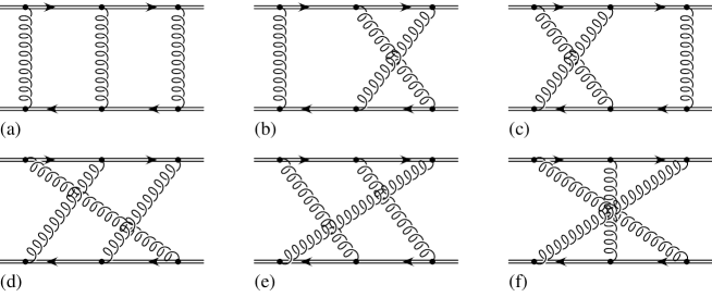
Figure 2: Two-loop ladder diagrams.

As has been demonstrated in [2], the consequence is that in order to compute the actual two-loop contribution to the potential, only those diagrams have to be considered which involve color factors different from $C_{F}^{3}$ and $C_{F}^{2}C_{A}$ and thus cannot result from iterations of the lower order diagrams. This means that for example the first three of the ladder diagrams in Fig. 2 and all graphs which are merely source self-energy insertions in one-loop graphs are irrelevant.

To be more specific, the following diagrams have to be calculated:

• The two-loop ladder diagrams Fig. 2(d-f).

• The corrections to the one-loop ladder diagrams shown in Fig. 3. In general there would be more graphs of this type containing the three gluon vertex, e.g., analogous to Fig. 3(c), which, however, vanish in Feynman gauge as already explained. In fact, Fig. 3(f) vanishes as well, but this is a consequence of considering the color-singlet state of the sources.

• Two-loop vertex and gluon self-energy corrections, where the number of diagrams is also reduced by our choice of gauge, and double insertions of the corresponding one-loop corrections.

• The graphs containing the four-gluon vertex with all ends attached to the sources vanish in Feynman gauge as well.

All other two-loop graphs are already accounted for by the exponentiation.

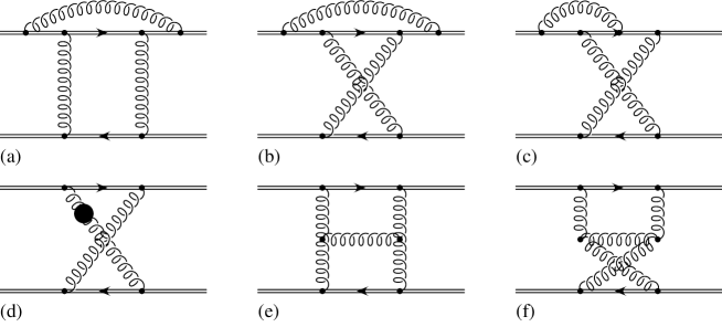
Figure 3: Corrections to one-loop ladder diagrams required for the potential calculation.

The relevant diagrams can be evaluated in momentum space without encountering any special difficulties. Using the integration by parts method [9], most of the integrals that occur can be reduced to products or convolutions of the standard one-loop two-point function, its HQET equivalent as given in [10], the HQET three-point function as given in [11] and the mixed-type three-point function

$$\overline{C}({\bf p}^{2})=\int\!\frac{d^{D}l}{(2\pi\mu)^{-2\epsilon}}\Big{(}\frac{-1}{l^{2}\!+\!i\epsilon}\Big{)}^{n}\!\Big{(}\frac{-1}{(l\!+\!p)^{2}\!+\!i\varepsilon}\Big{)}^{m}\!\Big{(}\frac{-1}{lv\!+\!i\varepsilon}\Big{)}^{a}$$

which can be computed by standard methods for $vp=0$. The diagrams 2(d–f), 3(e) and the vertex correction containing two three-gluon vertices, however, require the computation of some true two-loop integrals. As a detailed description of the calculation must be postponed to a future publication, we only mention that the computer program FORM [12] has been used for the evaluation of most of the diagrams and immediately present the results.

Combining the two-loop result with the tree-level and one-loop expressions, the effective coupling constant introduced above can be written as

$$\alpha_{\rm V}({\bf q}^{2})=\alpha_{\rm{}_{\overline{MS}}}({\bf q}^{2})\Bigg{\{}1+\frac{\alpha_{\rm{}_{\overline{MS}}}({\bf q}^{2})}{4\pi}\frac{31C_{A}-20T_{F}n_{f}}{9}$$ (11)

$$+\Big{(}\frac{\alpha_{\rm{}_{\overline{MS}}}({\bf q}^{2})}{4\pi}\Big{)}^{2}\Big{[}C_{A}^{2}\Big{(}\frac{4343}{162}+\frac{24\pi^{2}-\pi^{4}}{4}+\frac{22}{3}\zeta_{3}\Big{)}$$

$$\quad-C_{A}T_{F}n_{f}\Big{(}\frac{1798}{81}+\frac{56}{3}\zeta_{3}\Big{)}$$

$$\quad-C_{F}T_{F}n_{f}\Big{(}\frac{55}{3}-16\zeta_{3}\Big{)}+(T_{F}n_{f})^{2}\frac{400}{81}\Big{]}\Bigg{\}}.$$

By inserting the three-loop running coupling in the $\overline{\rm MS}$-scheme (the formula can be found, for example, in [13]), we thus obtain the three-loop potential, in the sense that the expression is correct up to a constant multiplying $\alpha_{\rm{}_{\overline{MS}}}^{3}$. The terms proportional to $C_{F}T_{F}$ and $T_{F}^{2}$ in (11) could have been obtained from the one- and two-loop gluon propagator, but the other two terms really required computing.

Eq. (11) can be used to determine the scheme-dependent coefficient $\beta_{2}$ of the $\beta$-function for the $V$-scheme, as defined by

$$\frac{1}{\alpha_{\rm V}}\frac{d\alpha_{\rm V}}{d\ln\mu^{2}}=-\sum_{n=0}^{\infty}\beta_{n}^{\rm(V)}\Big{(}\frac{\alpha_{\rm V}}{4\pi}\Big{)}^{n+1},$$ (12)

with the result (the first two coefficients, of course, coincide with those of the $\overline{\rm MS}$-scheme)

$$\beta_{2}^{\rm(V)} = \Big{(}\frac{618+242\zeta_{3}}{9}+\frac{11(24\pi^{2}-\pi^{4})}{12}\Big{)}C_{A}^{3}$$ (13)

$$-\Big{(}\frac{445+704\zeta_{3}}{9}+\frac{24\pi^{2}-\pi^{4}}{3}\Big{)}C_{A}^{2}T_{F}n_{f}$$

$$+\frac{2+224\zeta_{3}}{9}C_{A}(T_{F}n_{f})^{2}-\frac{686-528\zeta_{3}}{9}C_{A}C_{F}T_{F}n_{f}$$

$$+2C_{F}^{2}T_{F}n_{f}+\frac{184-192\zeta_{3}}{9}C_{F}(T_{F}n_{f})^{2}.$$

The relation between the two couplings can, of course, be inverted easily, yielding

$$\alpha_{\rm{}_{\overline{\rm MS}}}({\bf q}^{2})=\alpha_{\rm V}({\bf q}^{2})\Bigg{\{}1-\frac{\alpha_{\rm V}({\bf q}^{2})}{4\pi}\frac{31C_{A}-20T_{F}n_{f}}{9}$$ (14)

$$-\Big{(}\frac{\alpha_{\rm V}({\bf q}^{2})}{4\pi}\Big{)}^{2}\Big{[}C_{A}^{2}\Big{(}\frac{499}{162}+\frac{24\pi^{2}-\pi^{4}}{4}+\frac{22}{3}\zeta_{3}\Big{)}$$

$$\quad+C_{A}T_{F}n_{f}\Big{(}\frac{682}{81}-\frac{56}{3}\zeta_{3}\Big{)}$$

$$\quad-C_{F}T_{F}n_{f}\Big{(}\frac{55}{3}-16\zeta_{3}\Big{)}-(T_{F}n_{f})^{2}\frac{400}{81}\Big{]}\Bigg{\}}.$$

This formula could be used to improve the precision when extracting $\alpha_{\rm{}_{\overline{MS}}}(M_{Z}^{2})$ from measurements of the Wilson loop on the lattice [14].

For $N=3$ the results in actual numbers read

$$\alpha_{\rm V}({\bf q}^{2})=\alpha_{\rm{}_{\overline{MS}}}({\bf q}^{2})\Bigg{\{}1+\frac{\alpha_{\rm{}_{\overline{MS}}}({\bf q}^{2})}{\pi}\Big{(}2.583-0.278n_{f}\Big{)}$$ (15)

$$+\Big{(}\frac{\alpha_{\rm{}_{\overline{MS}}}({\bf q}^{2})}{\pi}\Big{)}^{2}\Big{(}39.650-4.147n_{f}+0.077n_{f}^{2}\Big{)}\Bigg{\}},$$

$$\alpha_{\rm{}_{\overline{MS}}}({\bf q}^{2})=\alpha_{\rm V}({\bf q}^{2})\Bigg{\{}1-\frac{\alpha_{\rm V}({\bf q}^{2})}{\pi}\Big{(}2.583-0.278n_{f}\Big{)}$$ (16)

$$-\Big{(}\frac{\alpha_{\rm V}({\bf q}^{2})}{\pi}\Big{)}^{2}\Big{(}26.303-1.277n_{f}-0.077n_{f}^{2}\Big{)}\Bigg{\}},$$

which shows that the coefficients of the second order terms are not small even for $n_{f}=5$.

I would like to thank Prof. J. H. Kühn for suggesting this problem to me and for carefully reading the manuscript. This work was supported by the “Landesgraduiertenförderung” at the University of Karlsruhe.

References

- [1] L. Susskind, Coarse grained quantum chromodynamics in R. Balian and C. H. Llewellyn Smith (eds.), Weak and electromagnetic interactions at high energy (North Holland, Amsterdam, 1977).
- [2] W. Fischler, Nucl. Phys. B129, 157 (1977).
- [3] T. Appelquist, M. Dine and I. J. Muzinich, Phys. Lett. 69B, 231 (1977).
- [4] T. Appelquist, M. Dine and I. J. Muzinich, Phys. Rev. D17, 2074 (1978).
- [5] A. Billoire, Physics Letters 92B, 343 (1980).
- [6] S. N. Gupta and S. F. Radford, Phys. Rev. D24, 2309 (1981).
- [7] W. Lucha, F. F. Schöberl and D. Gromes, Physics Reports 200, 127 (1989).
- [8] P. P. Kulish and L. D. Faddeev, Theo. Math. Phys. 4, 745 (1971); see also J. M. Jauch and F. Rohrlich, The Theory of Photons and Electrons 2nd ed. (Springer, New York, 1976) Supplement S4.
- [9] K. G. Chetyrkin and F. Tkachov, Nucl. Phys. B192, 159 (1981).
- [10] D. J. Broadhurst and A. G. Grozin, Phys. Lett. B267, 105 (1991).
- [11] E. Bagan, P. Ball and P. Gosdzinsky, Phys. Lett. B301, 249 (1993).
- [12] J. A. M. Vermaseren, Symbolic Manipulation with FORM (CAN, Amsterdam, 1991).
- [13] Review of Particle Properties, R. M. Barnett et al., Phys. Rev. D54, 1 (1996).
- [14] see for example P. McCallum and J. Shigemutsu, Nucl. Phys. B (Proc. Suppl.) 47, 409 (1996) and references therein.