Final state rescattering as a contribution to $B\to\rho\gamma$.

Abstract

We provide a new estimate of the long-distance component to the radiative transition $B\to\rho\gamma$. Our mechanism involves the soft-scattering of on-shell hadronic products of nonleptonic $B$ decay, as in the chain $B\to\rho\rho\to\rho\gamma$. We employ a phenomenological fit to scattering data to estimate the effect. The specific intermediate states considered here modify the $B\to\rho\gamma$ decay rate at roughly the $5\to 8\%$ level, although the underlying effect has the potential to be larger. Contrary to other mechanisms of long distance physics which have been discussed in the literature, this yields a non-negligible modification of the $B^{0}\to\rho^{0}\gamma$ channel and hence will provide an uncertainty in the extraction of $V_{td}$. This mechanism also affects the isospin relation between the rates for $B^{-}\to\rho^{-}\gamma$ and $B^{0}\to\rho^{0}\gamma$ and may generate CP asymmetries at experimentally observable levels.

I Introduction

The study of radiative rare decays of $B$ mesons can provide valuable information on certain parameters in the CKM matrix. In particular, $B\to\rho\gamma$ is thought to be an especially clean mode for extracting the $V_{td}$ matrix element.${}^{\cite[cite]{[\@@bibref{Number}{vtd}{}{}]}}$ Although not yet observed, this mode should be accessible for study at B-factories. However, the smallness of the short-distance $B\to\rho\gamma$ amplitude raises the concern that the experimental signal could be influenced by long-distance effects, with the possibility of their contributing a non-negligible fraction to the decay rate.

The first studies${}^{\cite[cite]{[\@@bibref{Number}{gp}{}{}]}}$ of long distance contributions to rare $B$ decays employed the vector meson dominance (VMD) model (cf Fig. 1(a)). As applied to the $B\to\rho\gamma$ transition,${}^{\cite[cite]{[\@@bibref{Number}{cheng}{}{}]}}$ this involves the decay $B\to\rho V^{*0}$ ($V^{*0}$ represents an off-shell neutral vector meson such as $\rho^{0},\omega,\phi,J/\psi,\dots$) with subsequent conversion of the vector meson to the photon. More recently, light-cone QCD sum-rules have been used to analyze the weak annihilation long-distance contribution to $B\to\rho\gamma$.${}^{\cite[cite]{[\@@bibref{Number}{lcsr}{}{}]}}$ Here, the main effect arises from direct emission of the final state photon from the light spectator quark in the $B$ meson followed by ${\bar{b}}q$ weak annihilation.

Both these approaches suffer from some degree of theoretical uncertainty. Besides the usual model dependence of these methods, in both cases no allowance is made for final state interactions (FSI). However, the $\rho\gamma$ decay mode can be generated by the decay of a B meson into a hadronic final state which then rescatters into $\rho\gamma$. It has recently been shown${}^{\cite[cite]{[\@@bibref{Number}{we}{}{}]}}$ that soft-FSI effects are ${\cal O}(1)$ in the large $m_{b}$ limit and cannot legitimately be ignored.

In this paper, we provide an estimate of a long distance component to $B\to\rho\gamma$ which deals solely with on-shell transition amplitudes while explicitly taking the occurrence of FSI into account. Our mechanism can be viewed as a unitarity analysis, where a $B$ decays into some intermediate state which then undergoes soft-rescattering into the final $\rho\gamma$ configuration. Of course, we are not able to account for all possible intermediate states, so that in order to provide a rough estimate for the the effect we must analyse a few specific contributions. For definiteness, we consider the $\rho^{0}\rho^{0}$ and $\rho^{+}\rho^{-}$ intermediate states in $B^{0}$ decay. In the language of Regge theory,${}^{\cite[cite]{[\@@bibref{Number}{we,collins}{}{}]}}$ the first of these proceeds by Pomeron exchange and is technically the dominant contribution, remaining nonzero in the heavy quark limit. However, the $\rho^{+}\rho^{-}$ contribution, whose rescattering is mediated by the $\rho$ trajectory and is thus nonleading, can be numerically important because $B^{0}\to\rho^{+}\rho^{-}$ is color-allowed (whereas $B^{0}\to\rho^{0}\rho^{0}$ is color-suppressed) and because the relatively low value of the $B$ mass turns out to blur somewhat the distinction between Regge-leading and nonleading contributions. Finally, since the corrections considered here are not themselves proportional to $V_{td}$, their presence constitutes a potential source of serious error in the phenomenological extraction of $V_{td}$.${}^{\cite[cite]{[\@@bibref{Number}{joao}{}{}]}}$ This underscores the importance of obtaining quantitative estimates of such effects.

II Soft hadronic rescattering

Effects of final state interactions (e.g. Fig. 1(b)) are naturally described using the unitarity property of the ${\cal S}$-matrix, ${\cal S}^{\dagger}{\cal S}=1$. This condition implies that the ${\cal T}$-matrix, ${\cal S}=1+i{\cal T}$, obeys

$${\cal D}isc~{}{\cal T}_{B\rightarrow f}\equiv{1\over 2i}\left[\langle f|{\cal T}|B\rangle-\langle f|{\cal T}^{\dagger}|B\rangle\right]={1\over 2}\sum_{I}\langle f|{\cal T}^{\dagger}|I\rangle\langle I|{\cal T}|B\rangle\ .$$ (1)

For the $B\to\rho\gamma$ transition the contribution from the $\rho$ intermediate state is the one which is most amenable to direct analysis, and we shall detail the $B\to\rho\rho\to\rho\gamma$ component throughout this paper. This encompasses the $\rho^{0}\rho^{0}$ and $\rho^{+}\rho^{-}$ intermediate states for $B^{0}$ decay and $\rho^{+}\rho^{0}$ for $B^{+}$ decay.

The final state interaction of Fig. 1(b) together with the unitarity condition implies a discontinuity relation for the invariant amplitude ${\cal M}_{B\to\rho\gamma}$,

$$2Disc~{}{\cal M}_{B\to\rho\gamma}^{\eta\theta}\epsilon^{*}_{\eta}(\lambda_{3})\epsilon^{*}_{\theta}(\lambda_{4})=$$ (5)

$$\int\frac{d^{4}p}{(2\pi)^{4}}(2\pi)^{2}~{}d_{\mu\nu}^{(1)}~{}\delta(p^{2}-m^{2})d_{\alpha\beta}^{(2)}~{}\delta((p_{B}-p)^{2}-m^{2}){\cal M}_{B\to\rho\rho}^{\mu\alpha}{\cal M}_{\rho\rho\to\rho\gamma}^{*~{}\nu\beta,\eta\theta}~{}\epsilon^{*}_{\eta}(\lambda_{3})\epsilon^{*}_{\theta}(\lambda_{4})$$

$$=\sum_{\lambda_{1},\lambda_{2}}\int\frac{d^{4}p}{(2\pi)^{4}}(2\pi)^{2}\delta(p^{2}-m^{2})\delta((p_{B}-p)^{2}-m^{2})$$

$$\phantom{xxxxxx}\times{\cal M}_{B\to\rho\rho}^{\mu\alpha}~{}\epsilon^{*}_{\mu}(\lambda_{1})\epsilon^{*}_{\alpha}(\lambda_{2})~{}\cdot\epsilon^{*}_{\nu}(\lambda_{1})\epsilon^{*}_{\beta}(\lambda_{2})~{}{\cal M}_{\rho\rho\to\rho\gamma}^{*~{}\nu\beta,\eta\theta}~{}\epsilon^{*}_{\eta}(\lambda_{3})\epsilon^{*}_{\theta}(\lambda_{4})\ ,$$

with $d^{(i)}_{\mu\nu}$ being the polarization tensors of $\rho$ mesons in the loop. When expressed in terms of helicity amplitudes, the above discontinuity formula simplifies to

$$2Disc~{}{\cal M}_{B\to\rho\gamma}(\lambda_{3}\lambda_{4})=$$ (7)

$$\sum_{\lambda_{1}\lambda_{2}}\int\frac{d^{4}p}{(2\pi)^{4}}(2\pi)^{2}\delta(p^{2}-m_{\rho}^{2})\delta((p_{B}-p)^{2}-m_{\rho}^{2}){\cal M}_{B\to\rho\rho}(\lambda_{1}\lambda_{2}){\cal M}^{*}_{\rho\rho\to\rho\gamma}(\lambda_{1}\lambda_{2};\lambda_{3}\lambda_{4})\ \ .$$

The FSI itself will arise from the scattering $\rho\rho\to\rho\gamma$. We shall employ the Regge-pole description for this rescattering process, requiring both Pomeron and $\rho$-trajectory contributions.

To begin, however, we recall from Regge phenomenology the well-known invariant amplitude for the scattering of particles with helicities $\{\lambda_{i}\}$,${}^{\cite[cite]{[\@@bibref{Number}{collins}{}{}]}}$

$${\cal M}_{i\rightarrow f}^{\lambda_{1}\lambda_{2};\lambda_{3}\lambda_{4}}=-\left(\frac{-t}{s_{0}}\right)^{m/2}~{}\frac{e^{-i\pi\alpha(t)}+{\cal J}}{2\sin\pi\alpha(t)}\gamma_{\lambda_{3}\lambda_{4}}^{\lambda_{1}\lambda_{2}}\left({s\over s_{0}}\right)^{\alpha(t)}\ \ ,$$ (8)

where $m=|\lambda_{3}-\lambda_{1}|+|\lambda_{4}-\lambda_{2}|$ and $|{\cal J}|=1$. In the $B\to\rho\rho$ weak decay, the $\rho\rho$ state can exist in any of three helicity configurations, $\lambda_{1}=\lambda_{2}=+1$, $\lambda_{1}=\lambda_{2}=-1$ and $\lambda_{1}=\lambda_{2}=0$ (or in obvious notation $++$, $--$ and $00$). Moreover, the Pomeron (and near $t=0$ also the leading $\rho$) exchange does not change the helicities of the rescattering particles, i.e. $\lambda_{1}=\lambda_{3},\lambda_{2}=\lambda_{4}$. In view of this and noting that the photon helicity must have $|\lambda_{\gamma}|=1$, we omit the $00$ helicity configuration from further consideration. This is equivalent to maintaining the condition of gauge invariance. Moreover, since parity invariance constrains the $++$ and $--$ helicity contributions to be equal, we drop the $\lambda_{1}\lambda_{2}$ superscript hereafter and take for the residue couplings $\gamma_{--}^{--}=\gamma_{++}^{++}\equiv\gamma$. Throughout we use the linear trajectory forms,

$$\alpha_{P}(t)=\alpha_{P}^{0}+\alpha_{P}^{\prime}t\ ,\qquad\alpha_{\rho}(t)=\alpha_{\rho}^{0}+\alpha_{\rho}^{\prime}t\ \ .$$ (9)

In the following discussion, we limit ourselves for clarity’s sake to $B^{0}\to\rho^{0}\gamma$ decay. The Pomeron part of the FSI occurs for the $\rho^{0}\rho^{0}$ intermediate state. We obtain

$$Disc~{}{\cal M}^{(P)}_{B^{0}\to\rho^{0}\gamma} = \frac{1}{16\pi s}{\cal M}_{B^{0}\to\rho^{0}\rho^{0}}\int^{0}_{t_{min}}\ dt\ {\cal M}_{\rho^{0}\rho^{0}\to\rho^{0}\gamma}^{*}$$ (10)

$$= -{\gamma_{P}\over 32\pi s}\left({s\over s_{0}}\right)^{\alpha_{P}^{0}}{\cal M}_{B^{0}\to\rho^{0}\rho^{0}}\int^{0}_{t_{min}}\ dt\ e^{\alpha_{P}^{\prime}\ln(s/s_{0})t}~{}\left(\cot[\pi\alpha(t)/2]+i\right)\ \ ,$$ (11)

where ${\cal J}=+1$ for Pomeron exchange. Observe that the cotangent factor will diverge at some $t=t_{0}$ such that $\alpha(t_{0})=0$. For the Pomeron, this occurs at $t_{0}\simeq-4.3$ GeV^-2, which lies outside the forward diffraction peak. Such spurious behavior has been well-known since the early days of Regge phenomenology and is avoidable by restricting the range of integration to the diffraction peak, by employing a modified ‘phenomenological’ amplitude or by invoking daughter trajectories to cancel the divergence. We adopt the first of these procedures and find

$$Disc~{}{\cal M}^{(P)}_{B^{0}\to\rho^{0}\gamma} = -{\gamma_{P}\over 32\pi}{s_{0}\over\alpha_{P}^{\prime}\ln(s/s_{0})}(0.26-0.92~{}i)\left({s\over s_{0}}\right)^{\alpha_{P}^{0}-1}{\cal M}_{B^{0}\to\rho^{0}\rho^{0}}$$ (12)

$$\equiv \epsilon_{P}\left(\frac{s}{s_{0}}\right)^{\alpha_{P}^{0}-1}{\cal M}_{B^{0}\to\rho^{0}\rho^{0}}\ \ ,$$ (13)

where $s_{0}\simeq 1$ GeV. The numerical quantity $\epsilon_{P}$ is defined to encode the strength of the Pomeron-mediated rescattering. We discuss later how to determine the Pomeron residue function $\gamma_{P}$ by fitting to experimental data.

The quantity $Disc~{}{\cal M}^{(P)}_{B^{0}\to\rho^{0}\gamma}$ must itself be inserted as input to a dispersion relation for ${\cal M}^{(P)}_{B^{0}\to\rho^{0}\gamma}$. Since the $s$-dependent factor in Eq. (13) is almost constant, the dispersion relation for the Pomeron contribution will require a single subtraction. Approximating $\alpha_{P}^{0}\simeq 1$, we have

$${\cal M}^{(P)}_{B^{0}\to\rho^{0}\gamma}(m_{B}^{2}) = {\cal M}^{(P)}_{B^{0}\to\rho^{0}\gamma}(0)+\frac{\epsilon_{P}}{\pi}{\cal M}_{B^{0}\to\rho^{0}\rho^{0}}m_{B}^{2}\int_{4m_{\rho}^{2}}^{\infty}\ \frac{ds}{s(s-m_{B}^{2})}$$ (14)

$$= {\cal M}^{(P)}_{B^{0}\to\rho^{0}\gamma}(0)+\frac{\epsilon_{P}}{\pi}{\cal M}_{B^{0}\to\rho^{0}\rho^{0}}\ln\Bigl{(}1-\frac{m_{B}^{2}}{4m_{\rho}^{2}}\Bigr{)}\ \ .$$ (15)

We now turn to the process $B^{0}\to\rho^{+}\rho^{-}\to\rho^{0}\gamma$. The formulas derived for the leading Pomeron contribution of Eq. (13) are readily applicable to this case if one replaces the Pomeron trajectory by the $\rho$ trajectory, but now with ${\cal J}=-1$. This yields for the discontinuity function

$$Disc~{}{\cal M}^{(\rho)}_{B^{0}\to\rho^{0}\gamma} = -{\gamma_{\rho}\over 16\pi s}\left({s\over s_{0}}\right)^{\alpha_{\rho}^{0}}{\cal M}_{B^{0}\to\rho^{+}\rho^{-}}\int^{0}_{t_{min}}\ dt\ e^{\alpha_{\rho}^{\prime}\ln(s/s_{0})t}\left(1+i\tan[\pi\alpha(t)/2]\right)\ \ ,$$ (16)

$$= -{\gamma_{/}rho\over 32\pi}{s_{0}\over\alpha_{\rho}^{\prime}\ln(s/s_{0})}(0.92-0.33~{}i)\left({s\over s_{0}}\right)^{\alpha_{\rho}^{0}-1}{\cal M}_{B^{0}\to\rho^{0}\rho^{0}}$$ (17)

$$\equiv \epsilon_{\rho}\left(\frac{s}{s_{0}}\right)^{\alpha_{\rho}^{0}-1}{\cal M}_{B^{0}\to\rho^{+}\rho^{-}}\ \ ,$$ (18)

where $\epsilon_{\rho}$ is analogous to the quantity $\epsilon_{P}$ of Eq. (13). The asymptotic behavior,

$${Disc~{}{\cal M}^{(\rho)}_{B^{0}\to\rho^{0}\gamma}\over{\cal M}_{B^{0}\to\rho^{+}\rho^{-}}}\sim\left({s\over s_{0}}\right)^{\alpha_{\rho}^{0}-1}\ \ ,$$ (19)

justifies in this case use of an unsubtracted dispersion relation for the amplitude,

$${\cal M}^{(\rho)}_{B^{0}\to\rho^{0}\gamma}(m_{B}^{2}) = \frac{\epsilon_{\rho}}{\pi}{\cal M}_{B^{0}\to\rho^{+}\rho^{-}}{1\over\pi}\int^{\infty}_{4m_{\rho}^{2}}ds\ \left({s\over s_{0}}\right)^{\alpha_{\rho}^{0}-1}~{}{1\over s-m_{B}^{2}}$$ (20)

$$\simeq \frac{\epsilon_{\rho}}{\pi}{\cal M}_{B\to\rho^{+}\rho^{-}}\int^{\infty}_{4m_{\rho}^{2}}\frac{ds}{\sqrt{s}(s-m_{B}^{2})}=\frac{\epsilon_{\rho}}{\pi}{\sqrt{s_{0}}\over m_{B}}\ln\frac{2m_{\rho}-m_{B}}{2m_{\rho}+m_{B}}~{}{\cal M}_{B^{0}\to\rho^{+}\rho^{-}}\ \ ,$$ (21)

where we approximate $\alpha_{\rho}^{0}\simeq 0.5$. The above discussion is extendable in like manner to $B^{+}\to\rho^{+}\gamma$ decay.

III The Weak Decay Vertex

The most general form for the weak amplitude $B\to\rho\rho$ is${}^{\cite[cite]{[\@@bibref{Number}{gv}{}{}]}}$

$${\cal M}_{B(p)\to\rho(k_{1})\rho(k_{2})}=\epsilon^{*\mu}(k_{2})\epsilon^{*\nu}(k_{1})\left[ag_{\mu\nu}+\frac{b}{m_{\rho}^{2}}p_{\mu}p_{\nu}+i\frac{c}{m_{\rho}^{2}}\epsilon_{\mu\nu\alpha\beta}k_{1}^{\alpha}p^{\beta}\right]\ \ .$$ (22)

The quantities $a,b,c$ can be interpreted as partial-wave amplitudes as they exhibit the respective threshold behavior of $S,D,P$-waves. To proceed further requires knowledge of $\{a,b,c\}$ for both the $B^{0}\to\rho^{0}\rho^{0}$ and $B^{0}\to\rho^{+}\rho^{-}$ weak decays. Since no data yet exists for the $B\to\rho\rho$ transitions, we must determine $\{a,b,c\}$ theoretically. We have employed the BSW description of the nonleptonic $B$ transitions.${}^{\cite[cite]{[\@@bibref{Number}{bsw}{}{}]}}$ In this model, the amplitude for the $B^{0}\rho^{+}\rho^{-}$ transition is

$${\cal M}_{B^{0}(p)\to\rho^{+}(k_{1})\rho^{-}(k_{2})}=\frac{G_{F}}{\sqrt{2}}V_{ub}V_{ud}^{*}~{}a_{1}~{}\langle\rho^{-}(k_{2})|\bar{d}\gamma^{\mu}u|0\rangle\langle\rho^{+}(k_{1})|\bar{u}\gamma_{\mu}(1+\gamma_{5})b|B^{0}(p)\rangle\ \ ,$$ (23)

where $a_{1}\simeq 1.03$.${}^{\cite[cite]{[\@@bibref{Number}{bhp}{}{}]}}$ We adopt standard notation for the matrix elements,

$$\langle\rho^{-}(k_{2})|\bar{u}\gamma^{\mu}d|0\rangle = f_{\rho}m_{\rho}\epsilon^{*\mu}(k_{2})$$ (24)

$$\langle\rho^{+}(k_{1})|\bar{u}\gamma_{\mu}b|B^{0}(p)\rangle = \frac{2i}{m_{B}+m_{\rho}}\epsilon_{\mu\nu\alpha\beta}\epsilon^{*\nu}(k_{1})k_{1}^{\alpha}p^{\beta}~{}V(k_{2}^{2})$$ (25)

$$\langle\rho^{+}(k_{1})|\bar{u}\gamma_{\mu}\gamma_{5}b|B^{0}(p)\rangle = (m_{B}+m_{\rho})\epsilon^{*}_{\mu}(k_{1})A_{1}(k^{2}_{2})-\frac{\epsilon^{*}(k_{1})\cdot k_{2}}{m_{B}+m_{\rho}}(p+k_{1})_{\mu}A_{2}(k_{2}^{2})$$ (26)

$$- \frac{2\epsilon^{*}(k_{1})\cdot k_{2}}{k_{2}^{2}}{k_{2}}_{\mu}m_{\rho}\Bigr{[}A_{3}(k_{2}^{2})-A_{0}(k_{2}^{2})\Bigr{]}\ \ .$$ (27)

In what follows we assume the $k_{2}^{2}$ behavior of the form factors to be of the simple pole form, and for $k_{2}^{2}=m_{\rho}^{2}$ we obtain

$$V(k_{2}^{2}) = {h_{V}\over 1-k_{2}^{2}/m_{B^{*}}^{2}}\simeq h_{V}$$ (28)

$$A_{i}(k_{2}^{2}) = {h_{A_{i}}\over 1-k_{2}^{2}/m_{B^{*}}^{2}}\simeq h_{A_{i}}\quad(i=0,\dots,3)\ ,$$ (29)

with $h_{V}\simeq 0.33,h_{A_{1}}\simeq h_{A_{2}}\simeq 0.28$.${}^{\cite[cite]{[\@@bibref{Number}{bsw}{}{}]}}$ This gives for the amplitudes in Eq. (22),

$$a \simeq \frac{G_{F}}{\sqrt{2}}V_{ub}V_{ud}^{*}m_{\rho}a_{1}f_{\rho}(m_{B}+m_{\rho})h_{A_{1}}\ ,$$ (30)

$$b \simeq -\frac{G_{F}}{\sqrt{2}}V_{ub}V_{ud}^{*}a_{1}f_{\rho}\frac{2m_{\rho}^{3}}{m_{B}+m_{\rho}}h_{A_{2}}\ ,$$ (31)

$$c \simeq \frac{G_{F}}{\sqrt{2}}V_{ub}V_{ud}^{*}a_{1}f_{\rho}\frac{2m_{\rho}^{3}}{m_{B}+m_{\rho}}h_{V}\ \ .$$ (32)

The set of relevant helicity amplitudes can be written using explicit form of the polarization vectors. The connection between the transverse helicity amplitudes and form factors in Eq. (22) is${}^{\cite[cite]{[\@@bibref{Number}{gp}{}{}]}}$

$${\cal M}^{++}_{\rho\rho}=a+\sqrt{x^{2}-1}~{}c\ ,\qquad{\cal M}^{--}_{\rho\rho}=a-\sqrt{x^{2}-1}~{}c$$ (33)

where $x\equiv(m_{B}^{2}-2m_{\rho}^{2})/2m_{\rho}^{2}$. For completeness, we note that branching ratios for the $B\to\rho\rho$ decays calculated from Eq. (33) amount to ${\cal B}_{\bar{B}^{0}\to\rho^{0}\rho^{0}}=4.8\cdot 10^{-7}$, ${\cal B}_{\bar{B}^{0}\to\rho^{+}\rho^{-}}=2.1\cdot 10^{-5}$ and ${\cal B}_{\bar{B}^{-}\to\rho^{-}\rho^{0}}=1.5\cdot 10^{-5}$, where all three $\rho\rho$ helicity configurations have been summed over.

IV Numerical Results

Before numerically estimating the long-distance effects in $B\to\rho\gamma$, we first recall the determination of the short-distance contribution which arises from the effective Hamiltonian${}^{\cite[cite]{[\@@bibref{Number}{lcsr}{}{}]}}$

$${\cal H}^{\rm s.d.} = \frac{G_{F}}{\sqrt{2}}\Bigl{(}V_{tb}V_{td}^{*}C_{7}^{\mbox{{eff}}}~{}O_{7}+\dots\Bigr{)}\ \ ,$$ (34)

$$O_{7} = \frac{em_{b}}{8\pi^{2}}\bar{d}\sigma_{\mu\nu}(1-\gamma_{5})F^{\mu\nu}b\ \ ,$$ (35)

where $C_{7}^{\mbox{eff}}=-0.306$. The amplitude for the short-distance $B\to\rho\gamma$ contribution is

$${\cal M}_{\rm s.d.}^{\lambda_{\gamma},\lambda_{\rho}}=$$ (37)

$$-\frac{G_{F}}{\sqrt{2}}V_{tb}V_{td}^{*}C_{7}^{\mbox{{eff}}}~{}\frac{em_{b}}{4\pi^{2}}~{}\epsilon^{*\mu}(q,\lambda_{\gamma})\epsilon^{*\nu}(k_{1},\lambda_{\rho})~{}2F^{\rm S}(0)\left[\epsilon_{\mu\nu\alpha\beta}k_{1}^{\alpha}p^{\beta}-i\left(m_{B}E_{\gamma}g_{\mu\nu}-p_{\mu}q_{\nu}\right)\right]\ ,$$

where $\lambda_{\gamma},\lambda_{\rho}$ are the respective photon, rho helicities and $F^{\rm S}(q^{2}=0)$ is a form factor related to the $B$-to-$\rho$ matrix element of $O_{7}$. It is estimated from QCD sum rules${}^{\cite[cite]{[\@@bibref{Number}{lcsr}{}{}]}}$ that $F^{\rm S}(0)\simeq 0.17$ for $B^{0}\to\rho^{0}\gamma$ and $F^{\rm S}(0)\simeq 0.17\sqrt{2}$ for $B^{-}\to\rho^{-}\gamma$. This $B\to\rho\gamma$ matrix element can be written in a form similar to Eq. (22) with the identification

$$a^{\rm s.d.} = i\frac{G_{F}}{\sqrt{2}}V_{tb}V_{td}^{*}C_{7}^{\mbox{{eff}}}~{}\frac{em_{b}}{2\pi^{2}}m_{B}E_{\gamma}F^{S}(0)$$ (38)

$$c^{\rm s.d.} = -b^{\rm s.d.}=i\frac{G_{F}}{\sqrt{2}}m_{\rho}^{2}V_{tb}V_{td}^{*}C_{7}^{\mbox{{eff}}}~{}\frac{em_{b}}{2\pi^{2}}F^{S}(0)\ \ .$$ (39)

These can be related to the set of helicity amplitudes by using Eq. (33) which then contribute to the decay rate for $B\to\rho\gamma$ as

$${\Gamma_{B\to\rho\gamma}}^{\rm s.d.}=\frac{|{\bf q}|}{8\pi m_{B}^{2}}\Bigl{(}|{\cal M}^{++}_{s.d.}|^{2}+|{\cal M}^{--}_{s.d.}|^{2}\Bigr{)}\ \ ,$$ (40)

where ${\bf q}$ is the photon momentum.

In our numerical work, we have adopted for the CKM matrix elements the values${}^{\cite[cite]{[\@@bibref{Number}{al}{}{}]}}$

$$|V_{cb}|=0.0393\ ,\quad|V_{ub}|=0.08~{}|V_{cb}|\ ,\quad 1.4\leq\bigg{|}{V_{td}\over V_{ub}}\bigg{|}\leq 4.6\ .$$ (41)

The biggest source of uncertainty for the short-distance contribution is clearly the magnitude of $V_{td}$. The above range leads to a range of branching ratios for the short distance component

$${\cal B}^{\rm s.d.}_{B^{0}\to\rho^{0}\gamma}\equiv{\Gamma^{\rm s.d.}_{B^{0}\to\rho^{0}\gamma}\over\Gamma^{\rm tot.}_{B^{0}}}\simeq 10^{-7}\longrightarrow 10^{-6}\ \ ,$$ (42)

with ${\cal B}^{\rm s.d.}_{B^{-}\to\rho^{-}\gamma}=2{\cal B}^{\rm s.d.}_{B^{0}\to\rho^{0}\gamma}$. It is this large theoretical spread which has motivated an experimental determination of ${\cal B}_{B\to\rho\gamma}$ as perhaps the best solution to the $V_{td}$ problem. At present, however, even the largest theoretical values are still considerably smaller than the experimental upper bounds ${\cal B}_{B^{0}\to\rho^{0}\gamma}\leq 3.9\times 10^{-5}$ and ${\cal B}_{B^{-}\to\rho^{-}\gamma}\leq 1.1\times 10^{-5}$.${}^{\cite[cite]{[\@@bibref{Number}{patt}{}{}]}}$

Upon including both short-distance and long-distance contributions, we obtain

$${\Gamma_{B\to\rho\gamma}}=\frac{|{\bf q}|}{8\pi m_{B}^{2}}\Bigl{(}|{\cal M}_{\rm s.d.}^{++}+{\cal M}_{\rm l.d.}^{++}|^{2}+|{\cal M}_{\rm s.d.}^{--}+{\cal M}_{\rm l.d.}^{--}|^{2}\Bigr{)}\ \ .$$ (43)

The long-distance amplitudes are in turn summed over contributions from the Pomeron and $\rho$ trajectories,

$${\cal M}_{\rm l.d.}^{\lambda_{1}\lambda_{2}}=\beta^{(P)}{\cal M}^{\lambda_{1}\lambda_{2}}_{\rho^{0}\rho^{0}}+\beta^{(\rho)}{\cal M}^{\lambda_{1}\lambda_{2}}_{\rho^{+}\rho^{-}}\ \ .$$ (44)

Using Eqs. (8),(11) and dropping the subtraction constant but keeping the terms which are clearly related to rescattering, we obtain

$$\beta^{(P)}=\frac{\epsilon_{P}}{\pi}\ln\Bigl{(}1-\frac{m_{B}^{2}}{4m_{\rho}^{2}}\Bigl{)}\ ,\qquad\beta^{(\rho)}=\frac{\epsilon_{\rho}}{\pi}{\sqrt{s_{0}}\over m_{B}}\ln\frac{2m_{\rho}-m_{B}}{2m_{\rho}+m_{B}}\ \ .$$ (45)

Also needed for estimation of the FSI effect are the residue functions $\gamma_{P}$ and $\gamma_{\rho}$. For the Pomeron case, we use experimental data on photoproduction of $\rho^{0}$ mesons from a nucleon target.${}^{\cite[cite]{[\@@bibref{Number}{photo}{}{}]}}$ Upon calculating the differential cross section $d\sigma/dt$ at $t\simeq 0$ from the matrix element of Eq. (8) and applying the quark-counting rule to relate Pomeron-$pp$ and Pomeron-$\rho\rho$ couplings, we obtain $\gamma_{P}\simeq 4.53$. Actually we use twice this value as the final-state photon can arise from either scattering vertex. For $\rho$ exchange, we use $\gamma p\to\rho^{+}n$ data${}^{\cite[cite]{[\@@bibref{Number}{rhopl}{}{}]}}$ together with the isospin relation $\gamma_{\rho}(\gamma\rho^{0}\to\rho^{+}\rho^{-})/\gamma_{\rho}(\gamma p\to\rho^{+}n)\simeq 2$ to obtain $\gamma_{\rho}\simeq 7.6$.

The recent review of the CKM matrix given in Ref. [11] cites $\rho=0.05$ and $\eta=0.36$ as providing the best fit to current data, where $\rho$ and $\eta$ are the Wolfenstein parameters

$$V_{ub}=A\lambda^{3}(\rho-i\eta)\ ,\qquad V_{td}=A\lambda^{3}(1-\rho-i\eta)\ \ ,$$ (46)

and which corresponds to $|V_{td}/V_{ub}|\simeq 2.8$. Assuming these central values, we obtain for the short distance and short-plus-long distance branching ratios the respective values

$${\cal B}^{\rm s.d.}_{B^{0}\to\rho^{0}\gamma}\simeq 7.3\times 10^{-7}\ ,\qquad{\cal B}^{\rm tot}_{B^{0}\to\rho^{0}\gamma}\simeq 7.8\times 10^{-7}\ \ .$$ (47)

Figure 2 displays the effect of varying the $\rho$, $\eta$ values over their allowed range${}^{\cite[cite]{[\@@bibref{Number}{al}{}{}]}}$. The upper and lower curves define the band of allowed values for the ratio $({\cal B}^{\rm tot}_{B^{0}\to\rho^{0}\gamma}-{\cal B}^{\rm s.d.}_{B^{0}\to\rho^{0}\gamma})/{\cal B}^{\rm s.d.}_{B^{0}\to\rho^{0}\gamma}$. The upper curve is seen to be about $8\%$ for virtually the entire physical range of $\rho$.

V Concluding Remarks

Final state rescattering effects may sometimes, although not always, modify the usual analysis of decay processes. The situations where rescattering can be important are those where there is a copiously produced final state which can rescatter to produce the decay mode being studied. In our case the most important channel is $B\to\rho^{+}\rho^{-}$, which is color allowed. It is also proportional to $V_{ub}$ instead of $V_{td}$ so that it is clearly a distinct contribution, and one that becomes more important if $V_{td}$ is at the lower end of its allowed range. Our results should also be adjusted upward or downward if the measured branching ratio proves to be larger or smaller than that predicted above using the BSW model.

The magnitude of the $\rho\rho\to\rho\gamma$ soft-scattering for $B^{0}\to\rho^{0}\gamma$, summarized in Eq. (47), is seen to occur at about the $8\%$ level. This differs from the QCD sum rule estimates of Ref. [4] which found a $10\%$ long distance contribution to ${\cal B}_{B^{+}\to\rho^{+}\gamma}$ but only a $1\%$ effect for ${\cal B}_{B^{0}\to\rho^{0}\gamma}$. Our result is especially noteworthy in view of the many other possible contributions to the unitarity sum and the finding of Ref. [5] that multi-particle intermediate states are likely to dominate. Thus, although it is not possible at this time for anyone to completely analyze the long distance component, it seems plausible that the FSI contribution has the potential to occur at the $10\%$ level and perhaps even higher. We concur with comments in the literature${}^{\cite[cite]{[\@@bibref{Number}{gp}{}{}]},\cite[cite]{[\@@bibref{Number}{lcsr}{}{}]},\cite[cite]{[\@@bibref{Number}{aap}{}{}]}}$ that a deviation from isospin relations based on the short distance amplitude (e.g. ${\cal B}_{B^{-}\to\rho^{-}\gamma}=2{\cal B}_{B^{0}\to\rho^{0}\gamma}$) will be evidence for a long distance component, and such is the case here. Defining a parameter $\Delta$ to measure the isospin violation as

$$\Delta\equiv 1-{1\over 2}{\Gamma_{B^{-}\to\rho^{-}\gamma}\over\Gamma_{B^{0}\to\rho^{0}\gamma}}\ \ ,$$ (48)

we display in Fig. 3 the dependence of the effect upon the Wolfenstein parameter $\rho$. The isospin violation is found to be largest for large $\rho$.

The FSI mechanism described here will not markedly affect the $B\to K^{*}\gamma$ rate. The leading CKM contribution would involve a $D_{s}^{*}-{\bar{D}}^{*}$ intermediate state and thus be very suppressed since the soft-scattering requires a Reggeon carrying the quantum numbers of the $D$ meson. The non-leading CKM amplitudes, involving contributions from light-quark intermediate states, are proportional to $V_{ub}$ and are likewise very suppressed.

Finally, we point out the implications of our work to obtaining a CP-violating signal. Since $B\to\rho\rho$ decay is governed by CKM matrix elements which differ from those describing the short distance $B\to\rho\gamma$ transition, the necessary condition for CP violation is satisfied. We consider the CP asymmetry

$$a=\frac{|\Gamma_{B\to\rho\gamma}-\Gamma_{\bar{B}\to\rho\gamma}|}{\Gamma_{B\to\rho\gamma}+\Gamma_{\bar{B}\to\rho\gamma}}=\frac{|{\cal B}_{B\to\rho\gamma}-{\cal B}_{\bar{B}\to\rho\gamma}|}{{\cal B}_{B\to\rho\gamma}+{\cal B}_{\bar{B}\to\rho\gamma}}\ \ .$$ (49)

We have studied the resulting effect numerically. The FSI are found to increase the amplitude for $B^{0}\to\rho^{0}\gamma$ but reduce it for ${\overline{B}}^{0}\to\rho^{0}\gamma$. This is what gives rise to the asymmetry and we find $a\simeq 7\%$. As with our other results, we take this magnitude as an indication that experimentally interesting signals might well exist and should not be ignored in planning for future studies.

We would like to thank João M. Soares for reading the manuscript and useful comments. This work was supported in part by the U.S. National Science Foundation.

FIG. 1.: $B\to\rho\gamma$ via (a) Vector dominance process and (b) final state interaction effect.

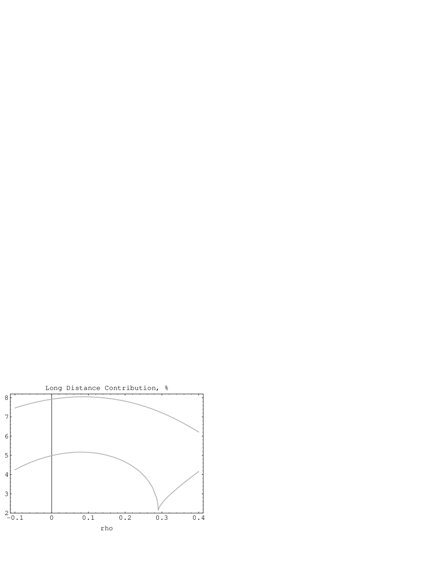
FIG. 2.: Dependence of the FSI effect upon the CKM parameter $\rho$.

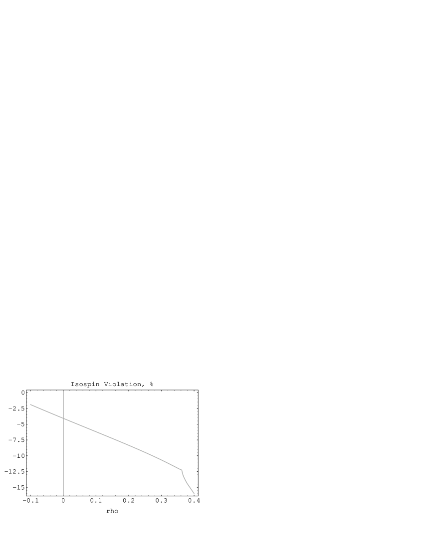
FIG. 3.: Dependence of isospin violation upon the CKM parameter $\rho$.

REFERENCES

• [1] A. Ali and C. Greub, Phys. Lett. B287 (1992) 191.
• [2] E. Golowich, S. Pakvasa Phys. Lett. B205 (1988) 393; Phys. Rev. D51 (1995) 1215.
• [3] H.-Y. Cheng Phys. Rev. D51 (1995) 6228. See also D. Atwood et al., Int. J. Mod. Phys. A11 (1996) 3743; N. Deshpande et al., Phys. Lett. B367 (1996) 362; J. Milana, Phys. Rev. D53 (1996) 1403.
• [4] A. Ali, V.M. Braun, Phys. Lett. B359 (1995) 223; A. Khodjamirian, G. Stoll and D. Wyler, Phys. Lett. B358 (1995) 129.
• [5] J.F. Donoghue, E. Golowich, A.A. Petrov, J.M. Soares, Phys. Rev. Lett. 77 (1996) 2178.
• [6] P.D.B. Collins, Introduction to Regge Theory and High Energy Physics, Cambridge Univ. Press, Cambridge, UK (1977).
• [7] J.M. Soares Phys. Rev. D49 (1994) 283.
• [8] G. Valencia, Phys. Rev. D39 (1989) 3339.
• [9] M. Wirbel, B. Stech, M. Bauer Z. Phys. C29 (1985) 637; ibid. C34 (1987) 103.
• [10] T. E. Browder, K. Honscheid, D. Pedrini, ‘Nonleptonic Decays and Lifetimes of $b$-quark and $c$-quark Hadrons’, Ann. Rev. Nucl. and Part. Sci. 46 (to appear).
• [11] A. Ali and D. London, ‘CP Violation and Flavour Mixing in the Standard Model – 1996 Update’, Preprint DESY-96-140, hep-ph/9607392.
• [12] ‘Radiative Penguin Decays of the $B$ Meson’, CLEO Collaboration Preprint CLEO CONF 96-05 (July 1996).
• [13] Yu. A. Alexandrov et al, Sov. J. Nucl. Phys., 32 (1980) 334.
• [14] D.P. Barber et al. Z. Phys. C2 (1979) 1.
• [15] B. Blok and I. Halperin, ‘Regge asymptotics and color suppressed heavy meson decays’, Preprint TECHNION-PHYS-96-14, hep-ph/9605441.
• [16] J.F. Donoghue and Alexey A. Petrov, Phys. Rev. D53 (1996) 3664.
Refer to caption