The hot baryon violation rate is $O(\alpha_{\rm w}^{5}T^{4})$

Abstract

The rate per unit volume for anomalous electroweak baryon number violation at high temperatures, in the symmetric phase, has been estimated in the literature to be $O(\alpha_{\rm w}^{4}T^{4})$ based on simple scaling arguments. We argue that damping effects in the plasma suppress the rate by an extra power of $\alpha_{\rm w}$ to give $O(\alpha_{\rm w}^{5}T^{4})$. We show how to understand this effect in a variety of ways ranging from an effective description of the long-distance modes responsible for baryon number violation, to a microscopic picture of the short-distance modes responsible for damping. In particular, we resolve an old controversy as to whether damping effects are relevant. Finally, we argue that similar damping effects should occur in numerical simulations of the rate in classical thermal field theory on a spatial lattice, and we point out a potential problem with simulations in the literature that have not found such an effect.

I Introduction

Anomalous baryon number (B) violation in the hot, symmetric phase of electroweak theory occurs through the creation of non-perturbative, nearly static, magnetic configurations with spatial extent of order $(g^{2}T)^{-1}$, where $g$ is the electroweak SU(2) coupling. (This is reviewed below.) It has been widely assumed that $g^{2}T$ must then be the only scale relevant to the problem, so that the baryon number violation rate per unit volume, by dimensional analysis, must be $O\bigl{(}(g^{2}T)^{4}\bigr{)}$. We shall argue that damping effects in the plasma cause the time scale for transitions through these configurations to be $O(g^{4}T)$ instead of $O(g^{2}T)$, and therefore the rate is $O\bigl{(}(g^{2}T)^{3}(g^{4}T)\bigr{)}=O(\alpha_{\rm w}^{5}T^{4})$.

The possible importance of damping effects was pointed out many years ago in ref. [3] in the context of B violation in the symmetry-broken phase of the theory. The effect was controversial, and another analysis of the problem [4] claimed that damping plays no role. In the intervening years, many people have privately expressed the concern that damping might affect the symmetric phase rate, and we make no claim to be the only, or even the first, people to think of it. The purpose of this paper is simply to resolve the controversy, elucidate the physics involved, and put to paper the result that the rate is $O(\alpha_{\rm w}^{5}T^{4})$. Many of the individual parts of this paper will be reviews of various aspects of thermal physics already familiar to some readers, but we believe their synthesis in this discussion of the baryon number violation rate is original.

In the remainder of this introduction we briefly review the conventional picture of anomalous transitions in the symmetric phase and the standard estimate of the rate. Then we give a quick but formal estimate of the effects of damping that closely follows the broken-phase discussion of damping in ref. [3].

The body of the paper is devoted to providing a number of different ways in which to understand the physics underlying this result. Section II begins with an analysis of the power spectrum of gauge field fluctuations based on the fluctuation-dissipation theorem and argues that it is fluctuations with frequency of order $g^{4}T$ and spatial extent $(g^{2}T)^{-1}$ which have sufficiently large amplitude to generate non-perturbative transitions. This is followed by a real-time, finite-temperature diagrammatic analysis which demonstrates that perturbation theory breaks down in exactly this domain due to the non-linear interactions of low-frequency, low-momentum components of the non-Abelian magnetic field. Then, in section III we sketch the microphysical origin of damping and turn to one of the traditional methods of understanding the transition rate: by computing the rate at which the system crosses the “ridge” separating classically inequivalent vacua. We show that a single net transition from the neighborhood of one valley to the next actually involves $O(1/g^{2})$ back-and-forth crossings of this ridge, and so standard methods which count individual ridge-crossings overcount the true rate by a factor of $1/g^{2}$—precisely the suppression due to damping. In the final section, we discuss how damping effects should also play a roll in the topological transition rate for classical thermal field theory on a spatial lattice. This appears inconsistent with the results of numerical simulations [5], which show no sign of damping effects. We explain why the simulations done so far may fail to measure the true topological transition rate.

This multiplicity of approaches in not intended to be a case of several poor arguments “substituting” for one good one. We believe that any one of the viewpoints discussed below provides compelling evidence that thermal damping is responsible for suppressing the high-temperature electroweak baryon violation rate by one power of $\alpha_{\rm w}$ relative to the naive order $\alpha_{\rm w}^{4}T^{4}$ estimate. Our goal is simply to examine the phenomena from multiple perspectives and understand the connections between them.

FIG. 1.: A schematic representation of the (bosonic) potential energy along a particular direction (labeled $z$) in field space, corresponding to topologically non-trivial transitions between vacua.

A Review of the standard picture

Fig. 1 is the standard visual aid for thinking about anomalous transitions. Consider the theory in Hamiltonian formalism or in $A_{0}=0$ gauge, where the degrees of freedom are ${\bf A}({\bf x})$ and the conjugate momenta are ${\bf E}({\bf x})=-\partial{\bf A}(x)/\partial t$. The horizontal axis represents one particular direction in the infinite-dimensional space of gauge configurations ${\bf A}({\bf x})$. The minima represent the vacuum ${\bf A}=0$ and large gauge transformations of it, labeled by their Chern-Simons number $N_{\rm cs}$. The vertical axis represents the potential energy of the configurations. Whenever a transition is made from the neighborhood of one minimum to another (which we call a topological transition), the electroweak anomaly causes baryon number to be violated by an amount proportional to $\Delta N_{\rm cs}$:

$$\Delta B\propto\Delta N_{\rm cs}=-{g^{2}\over 16\pi^{2}}\int d^{4}x\>{\rm tr}\,F\tilde{F}\,.$$ (1)

That said, we shall now ignore the fermions and, for simplicity, focus on the rate for topological transitions in the pure bosonic theory. And, since we are interested in the symmetric phase of the theory, we shall generally ignore the Higgs sector as well and focus on pure SU(2) gauge theory.

Topological transitions can occur at a significant rate if thermal fluctuations have enough energy to get over the top of the energy barrier separating neighboring vacua. The most important parameter determining the energy of the barrier is the spatial extent $R$ of the configurations depicted in fig. 1. In order to generate an $O(1)$ change in Chern-Simons number (or baryon number), Eq. (1) plus dimensional analysis implies that a gauge field of spatial extent $R$ must have a field strength of order $(gR^{2})^{-1}$. Consequently, the energy of these configurations on the potential energy barrier will be $O((g^{2}R)^{-1})$, while the gauge field amplitude itself (smoothed over the scale $R$) is $O((gR)^{-1})$.

So a more representative picture of the configuration space is provided by fig. 2a: the energy barrier is not a single point but a ridge which becomes arbitrarily low if arbitrarily large configurations are used to cross it. The smallest $R$ for which non-perturbative thermal transitions through such configurations are not significantly Boltzmann-suppressed is $R\sim 1/g^{2}T$. For the same reason, this is also the scale where perturbation theory breaks down in the hot plasma.

FIG. 2.: The same as fig. 1 but supplemented by an extra dimension of configuration space corresponding to (a) spatial size $R$ of the configurations, and (b) some other generic direction $y$, such as a particular mode of momentum $\sim T$.

$R\sim 1/g^{2}T$ is in fact the dominant spatial scale for topological transitions. One argument is entropy: there are fewer ways to cross the barrier with larger configurations than smaller ones. Another argument is due to magnetic confinement in the hot plasma. Ignore ${\bf E}=-\dot{\bf A}$ at the energy barrier for the moment, so that the configuration is purely magnetic. Though static non-Abelian electric forces are no longer confining at high temperature, static magnetic forces are. The confinement scale is just the spatial scale of non-perturbative physics, $1/g^{2}T$.

Now consider the transition rate. Suppose that a configuration of size $R$ on the energy barrier ridge of fig. 2a is produced in the plasma. What would be the time scale for its decay? The unstable modes of the configuration will be associated with momenta of order $1/R$. If the configuration were decaying at zero temperature, the time scale for decay would then be $O(1/R)$. So the standard estimate is that there is one unsuppressed transition per volume $R^{3}$ per time $R$, giving the rate $\Gamma\sim R^{-4}\sim(g^{2}T)^{4}$. As we shall see, the flaw in this estimate is that the configuration is not decaying at zero temperature but instead in interacting with the other excited modes of the plasma.

We should emphasize that the picture of fig. 2a is still incomplete because we have shown only two degrees of freedom in configuration space. There are an infinite number of other degrees of freedom in which the potential turns up so that, for fixed $R$, the energy barrier looks like a saddle as depicted in fig. 2b. The energy ridges discussed before are really hypersurfaces through configuration space, separating valleys that contain the different vacua. One can formally define these hypersurfaces as follows [4]: For each configuration ${\bf A}({\bf x})$, follow the steepest descent path away from it in the infinite-dimensional analog of fig. 2—that is, follow (minus) the gradient of the potential energy. For generic configurations, one will eventually approach one of the classical vacua. The barrier ridge hypersurface which separates the classical vacua is the exceptional hypersurface which doesn’t flow to a vacuum configuration. We shall return to this picture of the ridges in detail later, when we take up the old controversy about whether damping can affect the transition rate.

B A quick estimate of damping

Consider again the decay of a configuration ${\bf A}_{\rm b}({\bf x})$ of size $1/g^{2}T$ on the energy barrier. As the system passes through ${\bf A}_{\rm b}$, one may analyze the motion by linearizing the equation of motion. Expanding ${\bf A}({\bf x},t)={\bf A}_{\rm b}({\bf x})+\delta{\bf A}({\bf x},t)$, the equations have the form

$$\partial_{t}^{2}\,\delta{\bf A}({\bf x})={\bf J}({\bf x})-\hat{K}^{2}\,\delta{\bf A}({\bf x})+O(\delta{\bf A}^{2})\,,$$ (2)

where ${\bf J}$ is the gradient of the potential along the ridge and $\hat{K}^{2}$ is the potential energy curvature operator with a negative eigenvalue $-\kappa^{2}$ of order $(g^{2}T)^{2}$ corresponding to decay away from the ridge. For the moment, let’s focus on that one eigenmode, reducing our equation to

$$\partial_{t}^{2}\,\delta A=\kappa^{2}\,\delta A+O(\delta A^{2})\,.$$ (3)

The solution to this equation grows exponentially on a time scale of $1/g^{2}T$.

Now consider the interaction of this decay with typical thermal excitations of the plasma. The transition rate involves physics at soft energies $g^{2}T$ that are small compared to the hard energies $T$ of typical particles in the system. The simplest way to analyze the problem is to consider an effective theory for the soft modes of the theory, where the physics of the hard modes has been integrated out. In the context of (3), we need to know the effective $(\delta A)^{2}$ interaction generated by integrating out the hard modes. The soft-mode self-energy generated by the hard modes is dominated by the processes shown in fig. 3 and is known as the hard thermal loop approximation to the self-energy.

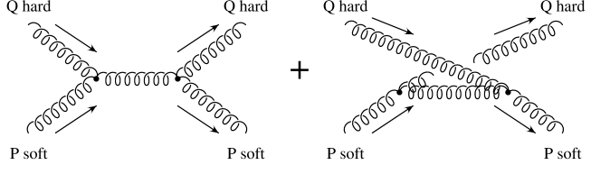
FIG. 3.: The soft-mode self-energy generated by forward scattering off of hard modes. The external hard lines are on-shell.

There is a reasonably simple formula for the resulting self-energy $\Pi(\omega,p)$ in the limit $\omega,p\ll T$ [9], but for our purposes it will only be important to know its qualitative behavior in terms of the ratio $\eta\equiv\omega/p$:

$$\Pi_{\rm L} = \cases{g^{2}T^{2}\,(O(1)-i\,O(\eta)),&$\eta\ll 1$ \,,\cr g^{2}T^{2}\,O(1),&$\eta\geq 1$ \,,\cr}$$ (5)

$$\Pi_{\rm T} = \cases{g^{2}T^{2}\,(O(\eta^{2})-i\,O(\eta)),&$\eta\ll 1$ \,,\cr g^{2}T^{2}\,O(1),&$\eta\geq 1$ \,,\cr}$$ (6)

where $\Pi_{\rm L}$ and $\Pi_{\rm T}$ are the longitudinal and transverse parts of the (retarded) one-loop self-energy. To distinguish them, it is convenient to momentarily switch to covariant gauge (rather than $A_{0}=0$ gauge), where the longitudinal and transverse projection operators are

$${\cal P}_{\rm L}^{\mu\nu} = -{P^{2}\over|{{\bf p}}|^{2}}\left(g^{\mu 0}-{P^{\mu}P^{0}\over P^{2}}\right)\left(g^{0\nu}-{P^{0}P^{\nu}\over P^{2}}\right)\,,$$ (8)

$${\cal P}_{\rm T}^{ij} = \delta^{ij}-{p^{i}p^{j}\over|{\bf p}|^{2}}\,,$$ (9)

where $P^{\mu}\equiv(\omega,{\bf p})$ and ${\cal P}_{T}$ has only spatial components. The $O(g^{2}T^{2})$ behavior of $\Pi_{\rm L}(0,{\bf p})$ reflects the Debye screening of static electric fields at distances of $1/gT$. The vanishing of $\Pi_{\rm T}(0,{\bf p})$ reflects the absence of similar screening for static magnetic fields. The $O(g^{2}T^{2})$ behavior of both $\Pi_{\rm T}(\omega,0)$ and $\Pi_{\rm L}(\omega,0)$ reflects the $O(gT)$ mass gap for propagating plasma waves.

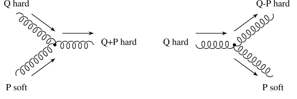
FIG. 4.: Absorption or emission of soft modes by hard modes when $\omega<p$, contributing to ${\rm Im}\Pi$.

The imaginary part of $\Pi_{\rm T}$ arises from absorption or emission due to scattering off hard particles in the thermal bath, as depicted in fig. 4. By kinematics, these processes occur only when $\omega<p$. Now modify eq. (3) to include the self-energy (and Fourier transform to frequency space),

$$-\omega^{2}\delta A=(\kappa^{2}-\Pi(\omega))\delta A\,.$$ (10)

Given that $\kappa\sim p\sim g^{2}T$, the self-energy $\Pi(\omega)$ will stabilize the unstable mode unless we focus on transverse modes and take $\eta\ll 1$. We may then approximate

$$\Pi\sim ig^{2}T^{2}\,\eta\sim i\,\omega T\,,$$ (11)

so that the solution to the linearized Eq. (10) is

$$\omega\sim ig^{4}T\,.$$ (12)

The decay time is therefore of order $1/g^{4}T$, or $1/g^{2}$ slower than assumed in the standard non-dissipative estimate.

II Some alternative views

A Analysis in terms of spectral density

We now consider another formal way to see that $\omega\sim g^{4}T$ is the appropriate frequency scale for topological transitions. Start by considering the power spectrum $\rho_{A}(\omega,{\bf p})$ of gauge-field fluctuations ${\bf A}(\omega,{\bf p})$ in the plasma:

$$\left\langle{\bf A}^{i}(\omega,{\bf p})^{*}{\bf A}^{j}(\omega^{\prime},{\bf p}^{\prime})\right\rangle\equiv\rho_{A}^{ij}(\omega,{\bf p})\,(2\pi)^{4}\delta(\omega{-}\omega^{\prime})\,\delta^{3}({\bf p}{-}{\bf p}^{\prime})\,.$$ (13)

This may be related to the retarded propagator

$$iD_{\rm R}^{ij}(t{-}t^{\prime},{\bf x}{-}{\bf x}^{\prime}) = \left\langle[{\bf A}^{i}(t,{\bf x})^{*},{\bf A}^{j}(t^{\prime},{\bf x}^{\prime})]\right\rangle\,\theta(t{-}t^{\prime})$$ (14)

$$= Z^{-1}\,{\rm Tr}\,e^{-\beta H}[{\bf A}^{i}(t,{\bf x})^{*},{\bf A}^{j}(t^{\prime},{\bf x}^{\prime})]\,\theta(t{-}t^{\prime})$$ (15)

by the fluctuation-dissipation theorem:

$$\rho_{A}(\omega,{\bf p})=-2(n_{\omega}+1)\,{\rm Im}D_{\rm R}(\omega,{\bf p})=-2(n_{\omega}+1)\,{\rm Im}\left(1\over(\omega+i\epsilon)^{2}-{\bf p}^{2}-\Pi(\omega,{\bf p})\right)\,,$$ (16)

where $n_{\omega}=1/(e^{\beta\omega}-1)$ is the Bose distribution function.

Now, using this relation, consider which frequencies of $A$ will have enough power to generate topological transitions. As reviewed in section 1, this requires fields with spatial extent $R\sim 1/g^{2}T$ and amplitude $A\sim 1/gR\sim gT$. Consider the right-hand side of (16) and use the hard thermal loop approximation (3) for $\Pi$ in

$${\rm Im}D_{\rm R}(\omega,{\bf p})={{\rm Im}\Pi\over(\omega^{2}-{\bf p}^{2}-{\rm Re}\Pi)^{2}+({\rm Im}\Pi)^{2}}~{}-~{}\delta\bigl{(}\omega^{2}-O(g^{2}T^{2})\bigr{)}$$ (17)

The last term corresponds to propagating plasma waves. For $p\sim g^{2}T$, the integrated power given by the right-hand side of (16) from all frequencies of order $\omega$ is of order

$$\omega\rho_{A}\sim\cases{1/g^{2}T\,,&$\omega\sim gT$ \,;\cr 1/\omega\,,&$g^{4}T\lesssim\omega\leq p$ \,;\cr\omega/g^{8}T^{2}\,,&$\omega\lesssim g^{4}T$ \,.\cr}$$ (18)

For $\omega\ll gT$, it is dominated by transverse fluctuations. A schematic plot of the power $\rho_{A}(\omega)$ is shown in fig. 5. From (13), the power in a particular soft mode with $R\sim 1/g^{2}T$, and frequency of order $\omega$, will produce fluctuations with amplitude

$$A\sim(p^{3}\omega\rho_{A})^{1/2}\sim\cases{g^{2}T\,,&$\omega\sim gT$ \,;\cr g^{3}\sqrt{T^{3}/\omega}\,,&$g^{4}T\lesssim\omega\leq p$ \,;\cr g^{-1}\sqrt{\omega T}\,,&$\omega\lesssim g^{4}T$ \,.\cr}$$ (19)

Hence, non-perturbative amplitudes $A\sim 1/gR\sim gT$ are generated when $\omega\sim g^{4}T$.

FIG. 5.: A schematic plot of the power $\rho_{A}(\omega)$ of gauge-field fluctuations with $p\sim g^{2}T$. The $\delta$-function spike at $\omega\sim gT$ corresponds to propagating plasmons.

In section 3, we shall see how to get this same power spectrum by considering the microphysical details of the behavior of the hard degrees of freedom, and we will translate the power spectrum into a qualitative discussion of what the actual real-time trajectories of the soft degrees of freedom look like.

B Estimate from Feynman diagrams

A pictorial way to represent the previous argument is to ask when diagrammatic perturbation theory breaks down in the effective theory of the soft modes, since we need non-perturbative effects for a topological transition. For simplicity, let us focus on transverse modes with $\omega\ll p$, for which one can ignore ${\rm Re}\Pi$. Consider adding a loop to a Feynman diagram, as shown in fig. 6, and consider the thermal contribution to that loop, shown in fig. 6c. The cost of adding the loop is order $(gp)^{2}$ from the new vertices, $p^{-4}$ from the two new uncut propagators, and $d^{3}p\,d\omega\>\rho_{A}(\omega,{\bf p})$ for the phase space probability of finding the new soft particle in fig. 6c, where $\rho_{A}\sim n_{\omega}\,{\rm Im}D_{\rm R}$. Integrating over frequencies of order $\omega$ and momenta of order $p\sim g^{2}T$, the cost of adding a loop is of order

$$(gp)^{2}\times p^{-4}\times p^{3}\omega\,{T\over\omega}\,{\rm Im}D_{\rm R}\sim g^{4}T^{2}\,{\rm Im}D_{\rm R}\sim\cases{g^{4}T/\omega\,,&$g^{4}T\lesssim\omega\leq p$ \,,\cr\omega/g^{4}T\,,&$\omega\lesssim g^{4}T$ \,.\cr}$$ (20)

So the loop expansion parameter is $O(1)$ for $\omega\sim g^{4}T$.

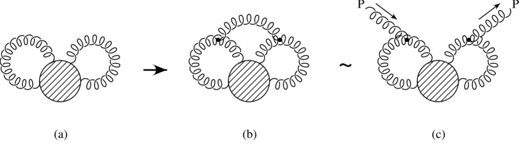
FIG. 6.: Adding a loop (a$\to$b) to a Feynman diagram. (c) represents the thermal contribution to the new loop, corresponding to forward scattering off a particle in the thermal bath.

C Interacting magnetic fields

Instead of considering Feynman diagrams in the effective theory (in which the self-energy has been resummed), we can get some insight into the origin of the transition time scale by recasting the above argument in terms of diagrams in the original, microscopic theory. The key to the estimates above was the behavior of ${\rm Im}\Pi_{\rm T}$, which arises from the interactions shown in fig. 4. The origin of the dominant contribution arising from multiple interactions of the form of fig. 6c is interactions such as those shown in fig. 7. The straight lines represent hard thermal particles; the wavy lines represent virtual magnetic quanta with $(\omega,p)\sim(g^{4}T,g^{2}T)$ that are absorbed or emitted.

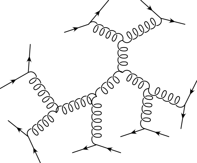
FIG. 7.: A microphysical picture of the important interactions for topological transitions.

The cost to the rate of adding a new interaction with a new hard particle is $(p^{-4})^{2}$ for new propagators, $(gp)^{2}$ for a new soft vertex, $(gT)^{2}$ for a new hard vertex, $O(1)$ for hard particle Bose or Fermi factors, and

$${d^{3}q\over 2\omega_{q}}{d^{3}q^{\prime}\over 2\omega_{q^{\prime}}}\;\theta(|{\bf q}{-}{\bf q}^{\prime}|\mathrel{\lesssim}p)\;\theta(|\omega_{q}{-}\omega_{q^{\prime}}|\mathrel{\lesssim}\omega)~{}\sim~{}T\omega p^{2}$$ (21)

for phase space. The total cost, by this estimate, is

$$(p^{-4})^{2}\times(gp)^{2}\times(gT)^{2}\times O(1)\times T\omega p^{2}\sim{\omega\over g^{4}T}$$ (22)

and is indeed $O(1)$ for $\omega\sim g^{4}T$. For larger $\omega$, where this microscopic perturbation theory appears to go completely wild, one must consider the effect of resumming the effects of ${\rm Im}\Pi$ into the soft propagators and return to our previous estimates. The advantage to having considered fig. 7 is simply that it gives us a physical picture for the origin of topological transitions in the plasma. The soft, virtual lines emitted from the hard particles simply correspond to the low-frequency and low-momentum components of the magnetic fields produced by the movement of those particles. These are not propagating electromagnetic waves but simply the magnetic fields carried by all moving charged particles. Topological transitions are then created by the non-linear interactions of these fields.

III Microphysical picture of barrier crossing

The normal approach used to calculate the topological transition rate in the symmetry-broken phase, and to estimate it in the symmetric phase, is based on calculating the rate, in equilibrium, at which the system crosses the energy barrier hypersurface separating the classical vacua [3, 4]. If one assumes that each such crossing is associated with a net transition of the system from the neighborhood of one vacuum to the neighborhood of another, then the barrier crossing rate is a good measure of the topological transition rate. Implicitly making this assumption, ref. [4] claimed to show that damping has no effect on topological transition rates, in contradiction to the claims of ref. [3]. In this section, we resolve this dilemma by showing that the assumed equality of the barrier crossing and net topological transition rates fails if one studies the full, short-distance theory. The difference in the rates will turn out to be precisely the suppression $\omega/g^{2}T\sim g^{2}$ we have argued arises from damping.

A Review of the microscopic origin of damping and the Langevin equation

Since the purpose of this paper is pedagogy and not excruciating details of formalism, we shall make some simplifications in order to elucidate the physics involved. First, we shall treat all the modes as classical and simply assume there is an ultraviolet cut-off at momenta of order $T$ (which is where quantum mechanics enters to cut off the ultraviolet catastrophe of classical thermal statistical mechanics). Secondly, though we shall consider all the hard modes of the theory, we shall only focus on the one soft mode ${\bf a}({\bf x})$ that is responsible for the decay of any particular configuration on the barrier. So we shall restrict $\delta{\bf A}(t,{\bf x})={\bf A}(t,{\bf x})-{\bf A}_{\rm b}({\bf x})$ to

$$\delta{\bf A}(t,x)\sim\delta A_{\rm soft}\;{\bf a}({\bf x})+\int_{\rm hard}d^{3}q\>\delta{\bf A}(t,{\bf q})\,e^{i{\bf q}\cdot{\bf x}}\,,$$ (23)

where the amplitude of ${\bf a}({\bf x})$ is normalized to $O(1)$ near its center. Finally, imagine putting the system in a box so that we can discretize the degrees of freedom. Rather than studying gauge theory directly, we shall begin by reviewing the derivation of damping for soft modes in a generic theory with cubic interactions:

$$\beta H={\textstyle{1\over 2}}p_{z}^{2}+{\textstyle{1\over 2}}K^{2}z^{2}+\sum_{i}\left(|p_{y_{i}}|^{2}+\Omega_{i}^{2}|y_{i}|^{2}\right)+z\sum_{ij}y_{i}^{*}{\cal G}_{ij}y_{j}\,.$$ (24)

Here $z$ represents the soft mode, $y_{i}$ the hard modes, $K^{2}\sim-(g^{2}T)^{2}$ the curvature of the potential energy for the unstable soft mode [but we could also consider stable soft modes with $K^{2}\sim+(g^{2}T)^{2}$], $\Omega_{i}$ the hard frequencies of order $T$, and ${\cal G}$ the soft-hard-hard part of the three-vector coupling.

The basic approximation is to realize that, provided the coupling ${\cal G}$ is perturbative, the motion of the many hard modes is not much affected by the motion of the soft mode. To first approximation, then,

$$y_{i}\simeq\alpha_{i}\,e^{-i\Omega_{i}t}\,,$$ (25)

where $\alpha_{i}$ are random phases and thermally-distributed random amplitudes:

$$\left\langle\alpha^{*}_{i}\alpha_{j}\right\rangle\equiv f(\Omega_{i})\,\delta_{ij}={1\over\Omega_{i}^{2}}\;\delta_{ij}\,,$$ (26)

which is the equipartition theorem with our normalizations (24). [With continuum normalizations, the quantity corresponding to $f(\Omega_{i})$ would be the classical limit $T/\Omega_{i}$ of the Bose distribution $n({\Omega_{i}})$.] Now consider the equation of motion for the mode of interest, $z$:

$$\ddot{z}+K^{2}z=-y^{*}{\cal G}y\,.$$ (27)

The leading approximation (25) produces an effectively random force term $\xi(t)$ on the right-hand side,

$$\xi(t)=-\sum_{ij}\alpha_{i}^{*}{\cal G}_{ij}\alpha_{j}\,e^{-i(\Omega_{j}-\Omega_{i})t}\,.$$ (28)

Using (26), the time correlation of this force is

$$\left\langle\xi(t)\xi(t{+}\Delta t)\right\rangle=\sum_{ij}f(\Omega_{i})f(\Omega_{j})\,|{\cal G}_{ij}|^{2}\,e^{-i(\Omega_{j}-\Omega_{i})\Delta t}\,.$$ (29)

The force $\xi(t)$ is therefore a source of colored noise for the evolution of the soft mode, and the power spectrum of that noise is given by the Fourier transform of (29):

$$\left\langle\xi(\omega)\xi(\omega^{\prime})\right\rangle=2\pi\delta(\omega{-}\omega^{\prime})\sum_{ij}f(\Omega_{i})f(\Omega_{j})\,|{\cal G}_{ij}|^{2}\,2\pi\delta(\Omega_{j}{-}\Omega_{i}{-}\omega)\,.$$ (30)

The square matrix element just represents the process of fig. 4 and, if one returns to continuum language, the power spectrum turns out to be simply

$$\left\langle\xi(\omega,{\bf p})\xi(\omega^{\prime},{\bf p}^{\prime})\right\rangle=-4\pi\delta(\omega{-}\omega^{\prime})\,\delta^{3}({\bf p}{-}{\bf p}^{\prime})\,n(\omega)\,{\rm Im}\Pi(\omega)\,.$$ (31)

So far we have reviewed the origin of an effectively random force term in the equation of motion for soft modes (a term that we did not discuss in our quick analysis of section 1). To see the origin of damping, one must consider the perturbative effect of the soft mode on the motion of the hard modes. The equations of motion for the $y_{i}$ are

$$\ddot{y}_{i}+\Omega_{i}^{2}\,y_{i}=-z(t)\sum_{j}{\cal G}_{ij}y_{j}\,.$$ (32)

The perturbation to the solution is easily obtained by using the free solution (25) for $y$ on the right-hand side and then Fourier transforming:

$$y_{i}(\omega)=\alpha_{i}\,2\pi\delta(\omega{-}\Omega_{i})+{1\over(\omega+i\epsilon)^{2}-\Omega_{i}^{2}}\sum_{j}{z(\omega{-}\Omega_{j})}{\cal G}_{ij}\alpha_{j}+O(z^{2})\,,$$ (33)

where we have used the retarded solution for the response of $y_{i}$ to $x$. Putting this solution into the soft-mode equation (27) now gives

$$\bigl{(}-\omega^{2}+K^{2}\bigr{)}z=\xi(\omega)+2\sum_{ijk}{\cal G}_{ij}{\cal G}_{jk}\,\alpha_{i}^{*}\alpha_{k}\,{z(\omega{+}\Omega_{i}{-}\Omega_{k})\over\omega^{2}-\Omega_{j}^{2}}+O(z^{2})\,.$$ (34)

Averaging the second term on the right-hand side over the random amplitudes $\alpha_{i}$ finally yields

$$\bigl{(}-\omega^{2}+K^{2}+\Pi(\omega)\bigr{)}z\simeq\xi(\omega)\,,$$ (35)

where

$$\Pi(\omega)=2\sum_{ij}f(\Omega_{i}){|{\cal G}_{ij}|^{2}\over(\omega+\Omega_{i}+i\epsilon)^{2}-\Omega_{j}^{2}}\,.$$ (36)

This is just the discretized version of the soft-mode self-energy of fig. 3.

The purpose of this review has been to show that the effective equation of motion (10), which we first used to argue that the decay time is $O(1/g^{4}T)$, should more accurately be a Langevin equation of the form

$$(-\omega^{2}+K^{2}+\Pi(\omega))\,\delta A_{\rm soft}=\xi(\omega)\,,$$ (37)

where $\xi(\omega)$ is a random force with $\langle\xi\rangle=0$ and power spectrum (31). For a stable soft mode ($K^{2}>0$), the decay of the mode due to the imaginary part of the $\Pi(\omega)\delta A$ term and the excitation of the mode by the random force term balance each other to maintain thermal equilibrium of the soft mode.

Now (dropping the subscript “soft”) consider the solution

$$\delta A(t)=\delta\bar{A}(t)+\Delta A(t)\,,$$ (38)

where $\delta\bar{A}(t)$ is the solution to the homogeneous equation that we originally considered in section 1 and $\Delta A(t)$ are the fluctuations induced by $\xi$:

$$\Delta A(\omega)={\xi(\omega)\over(-\omega^{2}+K^{2}+\Pi(\omega))}\,.$$ (39)

Computing the power spectrum of $\Delta A$ using (31), one recovers our earlier result of (16) for the power $\rho_{A}$, projected onto the soft mode under consideration.

B What does the decay look like?

Let’s now return to our characterization (18) of the power of the fluctuations in $A$ integrated over frequencies of order $\omega$. We’d now like to investigate how much the relevant soft mode oscillation $\Delta A(t)$ wiggles in time so that we can assess whether the barrier is crossed once or multiple times per net transition.

First, how many times does the motion of $\Delta A(t)$ change direction per unit time? This is equivalent to asking about the fluctuations in $\Delta\dot{A}(t)$. We can obtain the integrated power in $\dot{A}$ simply by multiplying (18) by $\omega^{2}$:

$$\omega\rho_{\dot{A}}\sim\cases{T\,,&$\omega\sim gT$ \,;\cr\omega\,,&$g^{4}T\lesssim\omega\leq p$ \,;\cr\omega^{3}/g^{8}T^{2}\,,&$\omega\lesssim g^{4}T$ \,.\cr}$$ (40)

Unlike the power for the amplitude $A$ of fluctuations, the power for $\dot{A}$ is dominated by plasma oscillations $\omega\sim gT$ and not by low frequencies $\omega\sim g^{4}T$. The time scale for the motion of $\Delta A(t)$ to change direction is therefore $1/gT$. The power in $\Delta A$ and $\Delta\dot{A}$ can be summarized by considering three characteristic frequency scales: $gT$, $g^{2}T$, and $g^{4}T$. The results of (18) and (40) are summarized for these scales in table I and depicted schematically in fig. 8. Remember that the oscillations $\Delta A$ are superimposed on top of the slow net motion of the homogeneous solution $\bar{A}$ for the damped decay.

$\omega$	$|A|$	$|\dot{A}|$
$gT$	$g^{2}T$	$g^{3}T^{2}$
$g^{2}T$	$g^{2}T$	$g^{4}T^{2}$
$g^{4}T$	$gT$	$g^{5}T^{2}$

TABLE I.: Amplitude of fluctuations in $A(t)$ and $\dot{A}(t)$ corresponding to three characteristic frequency scales.

FIG. 8.: A schematic picture of the time evolution of the fluctuations $\Delta A(t)$ showing fluctuations of scales $\omega\sim gT$, $g^{2}T$, and $g^{4}T$. Keep in mind, however, that there is really a spectrum of fluctuations between $\omega\sim g^{2}T$ and $\omega\sim g^{4}T$ whose amplitude grows as $\omega$ decreases.

Now let us estimate how many times the system crosses $\delta A=0$ during a topological transition. The time scale for the net transition is $t_{\rm net}\sim 1/g^{4}T$, over which $\delta A$ changes magnitude by $\delta_{\rm net}A\sim gT$. During that time, $\delta A(t)$ changes directions of order $gTt_{\rm net}\sim 1/g^{3}$ times due to plasma oscillations whose amplitude is $O(g^{2}T)$. The spectrum of fluctuations of the system may be rather complicated, but the total time the system spends within $O(g^{2}T)$ of $\delta A=0$ will be of order

$$t_{\rm net}\times{g^{2}T\over\delta_{\rm net}A}\sim{1\over g^{3}T}\,.$$ (41)

During this time, the plasma fluctuations are large enough to drive the system back and forth across $\delta A=0$ with frequency $gT$. Thus, during one net transition, the system crosses through $\delta A=0$ of order $1/g^{2}$ times. Any calculation which simply computes the rate of barrier crossing per unit time will overestimate the rate of net transitions by a factor of $1/g^{2}$.

C Being more precise about the “barrier”

In the previous section, we implied that crossing $\delta A_{\rm soft}=0$ many times during a transition implies that the energy barrier hypersurface is crossed many times during a transition. However, $\delta A_{\rm soft}$ is just the projection of ${\bf A}-{\bf A}_{\rm b}$ onto the soft mode of interest, and the exact equation for the energy barrier hypersurface is not really as simple as $\delta A_{\rm soft}=0$. Perhaps, as the hard modes oscillate, the $\delta A_{\rm soft}$ location of the barrier also oscillates. In order to confirm our picture, we should check that the effect of hard modes of the shape of the barrier is small enough not to affect our argument. We verify this in Appendix A.

IV Implications for classical lattice thermal field theory

The estimates of damping we have made have all been based on continuum, quantum, thermal field theory, where the effective ultraviolet cut-off for any thermal effects is $O(T)$, since the distribution of particles with momenta $\gg T$ is Boltzmann suppressed. One of the numerical testing grounds used in the literature for studying topological transition rates, however, has been classical thermal field theory on a spatial lattice. In classical thermal field theory, modes of arbitrarily high momenta are thermally excited (leading to the ultraviolet catastrophe of the classical blackbody problem), and the ultraviolet cut-off is the inverse lattice spacing $a^{-1}$ rather than $T$. As we shall argue below, this infinite growth in the number of relevant hard modes as $a\to 0$ leads to infinitely strong damping of the transition rate in the continuum limit of classical thermal field theory.

In the limit $\omega,p\ll T$, the usual continuum result for the imaginary part of the transverse self-energy $\Pi_{\rm T}$ from figs. 3 and 4 is of the form

$${\rm Im}\Pi_{\rm T}(\omega,{\bf p}) \sim g^{2}\int{d^{3}q\over 2|{\bf q}|}\>n_{q}\left[|{\cal M_{\omega}}|^{2}-|{\cal M}_{-\omega}|^{2}\right]\delta(\omega|{\bf q}|-{\bf p}\cdot{\bf q})$$ (42)

$$\sim g^{2}\,{\omega\over p}\int_{0}^{\infty}dq\>qn_{q}$$ (43)

$$\sim g^{2}T^{2}\,{\omega\over p}\,,$$ (44)

where ${\cal M}_{\omega}$ is the vertex in the left-hand figure of fig. 3. The $q$ integral is dominated by the ultraviolet and cut-off by $q\sim T$ for the quantum case, shown above.

For classical field theory, the only difference is that

$$n_{{\bf q}}\to{T\over\omega_{{\bf q}}}$$ (45)

and the ultraviolet cut-off is now the inverse lattice spacing $a^{-1}$, so that the last step of (44) now gives

$${\rm Im}\Pi_{\rm cl}(\omega,p)\sim g^{2}Ta^{-1}\,{\omega\over p},\qquad(\omega\ll p)\,.$$ (46)

Damping will therefore suppress the transition rate by an extra factor of $aT$ compared to the quantum field theory case, so that the rate is $O(\alpha^{5}aT^{5})$ and vanishes in the $a\to 0$ limit.

This result is in apparent contradiction with the numerical results of ref. [5], which claimed to find $O(\alpha^{4}T^{4})$ behavior for the rate. Our result is suppressed by an additional factor of $O(\alpha aT)$, which is one power of the dimensionless lattice coupling $\beta$. Ref. [5] used values of $\beta$ ranging from 10 to 14, so they should find a 40% violation of the assumed $O(\alpha^{4}T^{4})$ scaling of the rate. Such an effect is clearly inconsistent with their statistical errors. (See their fig. 3.)

There is a possible problem, however, with the assumption that ref. [5] is in fact measuring the topological transition rate. The problem stems from the subtleties of trying to define topological winding number on the lattice. The idea in ref. [5] was to measure a lattice analog of the square of the topological winding:

$$\left\langle\left(\int_{0}^{t}dt\int d^{3}x\>{\rm tr}F\tilde{F}\right)^{2}\right\rangle=\left\langle\left(\Delta N_{\rm cs}(t)\right)^{2}\right\rangle\,,$$ (47)

where it is now convenient to consider field strengths normalized so that the action is $F_{\mu\nu}^{2}/g^{2}$. Under the picture of fig. 1, the topological winding in pure gauge theory should randomly diffuse away from zero, so that at large times (47) behaves like $\Gamma Vt$ where $\Gamma$ is the transition rate. The authors implement this procedure on the lattice by making a lattice approximation to ${\rm tr}F\tilde{F}$, which schematically has the form of the cross-product

$${\rm tr}F\tilde{F}\to E^{a}\times{\rm tr}(U\sigma^{a})\equiv J\,,$$ (48)

where $U$ represents plaquettes perpendicular to the links the electric field $E$ lives on. (See ref. [5] for the detailed expression.) The potential problem with this representation is that, unlike the continuum expression for ${\rm tr}F\tilde{F}$, the integral (i.e., lattice sum) of $J$ over space is not a total time derivative. The time integral of this lattice analog to $\int d^{3}x\>{\rm tr}F\tilde{F}$ does not just depend on the initial and final configurations but depends on the path used to get from one to another. In particular, consider a path in time that starts from some configuration near the vacuum, never makes any non-perturbative excursions from it (and so in particular never makes a topological transition), and finally ends up back at the initial configuration. The lattice analog of the left-hand side of (47), $\left(\int dt\;d^{3}x\>J\right)^{2}$, would not be zero. Perturbative fluctuations can therefore either increase or decrease $\int dt\,d^{3}x\>J$ without increasing the energy, and so there will be a purely perturbative contribution to the diffusion.

To estimate the size of this lattice artifact in the diffusion rate $\Gamma$, consider expanding (48) in powers of the lattice spacing $a$ in lattice perturbation theory, remembering that $U\sim e^{ia^{2}B}$. The leading $E\cdot B$ term is a total time derivative and does not cause problems. As an example of a subleading term, consider a term involving $E$ and three powers of $B$:

$${\rm tr}F\tilde{F}\to{\rm tr}F\tilde{F}+a^{4}EBBB+\cdots$$ (49)

Now consider the contribution of this term in the right-hand side of (47):

$$a^{8}\int_{0}^{t}dt_{1}\int_{0}^{t}dt_{2}\left\langle\left(\int d^{3}x\>EBBB\right)_{t_{1}}\left(\int d^{3}x\>EBBB\right)_{t_{2}}\right\rangle$$ (50)

The correlation is dominated by the ultraviolet and will be quasi-local in space and time. So, in the large time limit, it becomes

$$a^{8}Vt\int dt^{\prime}\,d^{3}x\left\langle\left(EBBB\right)_{0,0}\left(EBBB\right)_{t^{\prime},{\bf x}}\right\rangle\sim\beta^{-4}a^{-4}Vt\sim g^{8}T^{4}Vt$$ (51)

This lattice artifact therefore gives a contribution to the measured diffusion rate $\Gamma$ of $O(\alpha^{4}T^{4})$. The moral is that purely perturbative effects, having nothing to do with true topological transitions, might obscure the true topological transition rate, which we have argued is $O(\alpha^{5}aT^{5})$.

This work was supported by the U.S. Department of Energy, grant DE-FG06-91ER40614. We would like to thank Jan Ambjørn, Patrick Huet, Alex Krasnitz, Larry McLerran, Misha Shaposhnikov, and Frank Wilczek for useful conversations (some of which date back ten years).

A Hard mode effects on the barrier surface shape

As discussed in section 1, the barrier hypersurface is the surface which (1) separates the vacua and (2) maps into itself when the gradient of the potential is followed. In this appendix, we want to focus on whether the hard modes have a significant impact on the shape of the surface. Specifically, consider (a) one soft, unstable mode of interest, and (b) all hard modes, as in the generic model of (24) with $K^{2}=-\kappa^{2}<0$. What is the equation of the barrier hypersurface in this subspace?

We shall restrict attention to typical hard mode amplitudes in the thermal bath, i.e., $|y_{i}|\sim 1/\Omega_{i}$. Secondly, we shall assume that the interaction ${\cal G}$ between the soft mode and any individual hard mode is perturbative, as it indeed is hot gauge theory. The translation of this condition to the generic model (24) is easily made by considering stable soft modes, in which case $|z|$ is typically $1/\kappa$ and our perturbative condition is $xy{\cal G}y\ll 1$, giving ${\cal G}\ll\kappa\Omega^{2}$.

Under these conditions, our result for the ridge equation is

$$z=\sum_{ij}y_{i}^{*}{{\cal G}_{ij}\over\Omega_{i}^{2}+\Omega_{j}^{2}}\,y_{j}\equiv{\bf y}^{*}S{\bf y}\,.$$ (A1)

This is easily checked as follows. First, it contains $(z,{\bf y},{\bf y}^{*})=(0,{\bf 0},{\bf 0})$ as it should. Next, we must check that

$$\nabla V(z,{\bf y}^{*},{\bf y})=(-\kappa^{2}z+{\bf y}^{*}{\cal G}{\bf y},\Omega^{2}{\bf y}+z{\cal G}{\bf y},{\bf y}^{*}\Omega+z{\bf y}^{*}G)$$ (A2)

lies in the tangent plane to the surface (within our approximations). On the surface (A1),

$$\nabla V(z,{\bf y}^{*},{\bf y})\simeq({\bf y}^{*}{\cal G}{\bf y},\Omega^{2}{\bf y},{\bf y}^{*}\Omega^{2})\,.$$ (A3)

The tangent plane to the surface is spanned by

$${d\over dy_{i}^{*}}(z({\bf y}^{*},{\bf y}),{\bf y}^{*},{\bf y})=\left((S{\bf y})_{i},\hat{{\bf e}}_{i},0\right)\,,$$ (A4)

$${d\over dy_{i}}(z({\bf y}^{*},{\bf y}),{\bf y}^{*},{\bf y})=\left((S{\bf y})_{i},0,\hat{{\bf e}}_{i}\right)\,,$$ (A5)

and so

$$n=(1,-S{\bf y},-{\bf y}^{*}S)$$ (A6)

is normal to the surface. (A3) and (A6) then give $n^{*}\cdot\nabla V\simeq 0$ as desired.

To count the number of barrier crossings in section 3, we should really have studied the evolution of $z-{\bf y}^{*}S{\bf y}$ rather than the evolution of $z$. We are now in a position to check whether this makes any difference by checking the amplitude of the fluctuations in ${\bf y}^{*}S{\bf y}$. Using the leading-order behavior (25) for the $y_{i}$ and averaging over the amplitudes yields the equal time amplitude

$$\left\langle({\bf y}^{*}S{\bf y})^{2}\right\rangle=\sum_{ij}f(\Omega_{i})f(\Omega_{j})|S_{ij}|^{2}\,.$$ (A7)

Comparing this to

$$\left\langle\xi^{2}\right\rangle=\sum_{ij}f(\Omega_{i})f(\Omega_{j})|G_{ij}|^{2}\,.$$ (A8)

shows that (A7) is of order $\langle\xi^{2}\rangle$ times the typical size of $\Omega^{-4}$ (which is $T^{-4}$). The continuum version is that the equation for the barrier surface is

$$\delta A=\chi({\bf A}_{\rm hard}(t))$$ (A9)

where

$$\langle\chi\rangle=0,\qquad\langle\chi^{2}\rangle\sim T^{-4}\langle\xi^{2}\rangle$$ (A10)

and $\xi$ here is understood to be projected onto the soft mode. Using (31) and $p\sim g^{2}T$,

$$\langle\chi^{2}\rangle\sim T^{-4}p^{3}\int d\omega\>n_{\omega}\,{\rm Im}\Pi(\omega)\sim T^{-4}p^{3}\times g^{2}T^{3}\sim(g^{4}T)^{2}\,.$$ (A11)

This $O(g^{4}T)$ magnitude of the fluctuations in the location of the surface is much smaller than the magnitude $g^{2}T$ plasma oscillations described in section 3. The shape of the surface therefore has no effect on our previous discussion of crossing the barrier.

REFERENCES

- [1] K. Kajantie, M. Laine, K. Rummukainen, and M. Shaposhnikov, CERN report CERN-TH/96-126, hep-ph/9605288.
- [2] S. Elitzur, Phys. Rev. D12, 3978 (1975).
- [3] P. Arnold and L. McLerran, Phys. Rev. D36, 581 (1987).
- [4] S. Khlebnikov and M. Shaposhnikov, Nucl. Phys. B308, 885 (1988).
- [5] J. Ambjørn and A. Krasnitz, Phys. Lett. B362, 97 (1995).
- [6] N. Christ, Phys. Rev. D21, 1591 (1980).
- [7] T. Appelquist and R. Pisarski, Phys. Rev. D23, 2305 (1981); S. Nadkarni, Phys. Rev. D27, 917 (1983); Phys. Rev. D38, 3287 (1988); Phys. Rev. Lett. 60, 491 (1988); N. Landsman, Nucl. Phys. B322, 498 (1989); K. Farakos, K. Kajantie, M. Shaposhnikov, Nucl. Phys. B425, 67 (1994).
- [8] E. Braaten and R. Pisarski, Phys. Rev. D45, 1827 (1992); Nucl. Phys. B337, 569 (1990).
- [9] H. Weldon, Phys. Rev. D26, 1394 (1982); U. Heinz, Ann. Phys. (N.Y.) 161, 48 (1985); 168, 148 (1986).
- [10] A. Fetter and J. Walecka, Quantum theory of Many-Particle Systems (McGraw-Hill: 1971).