DTP/96/66

hep-ph/9609474

The One-loop QCD Corrections for $\gamma^{*}\to Q\bar{Q}q\bar{q}$
E. W. N.  Glover and D. J. Miller
Physics Department, University of Durham,
Durham DH1 3LE, England

September 1996

We present the first calculation of the one-loop QCD corrections for the decay of an off-shell vector boson with vector couplings into two pairs of quarks of equal or unequal flavours keeping all orders in the number of colours. These matrix elements are relevant for the calculation of the next-to-leading order ${\cal O}(\alpha_{s}^{3})$ corrections to four jet production in electron-positron annihilation, the production of a gauge boson accompanied by two jets in hadron-hadron collisions and three jet production in deep inelastic scattering. We compute the interference of one-loop and tree level Feynman diagrams, and organise the matrix elements in terms of combinations of scalar loop integrals that are well behaved in the limit of vanishing Gram determinants. The results are therefore numerically stable and ready to be implemented in next-to-leading order Monte Carlo calculations of the $e^{+}e^{-}\to 4~{}{\rm jet}$, $e^{\pm}p\to e^{\pm}+3~{}{\rm jet}$ and $p\bar{p}\to V+2~{}{\rm jet}$ processes.

An important ingredient in the confrontation of hadronic jet data from high energy particle collisions with theoretical calculations in perturbative QCD is the calculation of parton level cross sections beyond leading order. This is so for a variety of reasons. First, the dependence on the unphysical renormalisation and factorisation scales is usually reduced. Second, the addition of more particles into the final state makes the calculation more sensitive to the details of the experimental jet algorithm. Third, the final state phase space is enlarged so that lowest order constraints on the jet transverse energy or rapidity are relaxed. Together, these improvements make for a more stable calculation that is better matched to the experimental data. Finally, the presence of large infrared logarithms can be detected and the appropriate resummations performed. In this paper, we present the first calculation of the one-loop matrix elements for a virtual gauge boson decay into two pairs of equal or unequal flavour quarks keeping all terms in the number of colours. These matrix elements are one of the ingredients of the next-to-leading order calculation relevant for the processes

• $e^{+}e^{-}\to 4~{}{\rm jets}$

• $e^{\pm}p\to e^{\pm}+3~{}{\rm jets}$

• $p\bar{p}\to V+2~{}{\rm jets}$ with $V=W$ or $Z$,

which have been observed in abundance in experiments at the major accelerators, LEP at CERN, HERA at DESY and the TEVATRON at Fermilab. In electron-positron collisions, applications include more precise measurements of the colour casimirs $C_{A}/C_{F}$ and $T_{F}/C_{F}$ and a reduction of the theoretical error in the extraction of the $WW$ cross section near threshold.

In recent years there have been several significant technical advances in one-loop Feynman diagram calculations, some relying on insight from supersymmetry and others inspired more directly by the superstring [1]. Most important has been the continuation of the one-loop scalar pentagon integral in 4-dimensions [2] to $D=4-2\epsilon$ dimensions [3, 4, 5]. At the same time, methods utilised in tree level matrix element calculations, colour decompositions and helicity have been taken over. To make best use of the helicity method, relations have been provided between conventional dimensional regularisation, where all polarisations and spinors are treated in $D$-dimensions, and other schemes where parts of the calculations are performed in 4-dimensions [6, 7]. With these technological improvements, compact one-loop helicity amplitudes for processes involving five partons have been presented by Bern, Kosower and Dixon [8, 9] and Kunszt, Signer and Trocsanyi [10, 11, 12], while recently, one of the helicity amplitudes for the leading colour part of the $Z\to q\bar{q}gg$ process has been evaluated [13]. Recently, Dixon and Signer have reported first numerical results for the leading colour contribution to the $e^{+}e^{-}\to 4~{}{\rm jet}$ rate at next-to-leading order [14]. As expected, the agreement between theory and experiment is significantly improved. Our results presented here can therefore provide a numerical check of the one-loop leading colour contribution from the four quark process.

For our calculation involving a massive external gauge boson, we choose to compute the interference between the tree-level and one-loop amplitudes directly. The resulting ‘squared’ matrix elements involve only dot products of the particle four-momenta in addition to the normal logarithms and dilogarithms encountered in one-loop Feynman diagram calculations. As a consequence, we can immediately eliminate all integrals more complicated than a scalar pentagon, although some box tensor-integrals with three loop momenta remain. We have kept all quantities in $D$-dimensions as in conventional dimensional regularisation, but have checked that the ’t Hooft-Veltman scheme [16] gives identical results [6, 7]. Throughout we reorganise the tensor loop integrals as combinations of scalar integrals using a momentum decomposition [17] (rather than the reciprocal momentum basis of [18, 5, 12]). The usual problem with this approach is the occurence and proliferation of Gram determinants ($\Delta$) in the denominator which both increases the size of the algebraic expressions and introduces numerical instabilities as $\Delta\to 0$. We have avoided this by introducing combinations of scalar loop integrals in groups that are finite in the limit that the Gram determinants vanish [8, 9, 10, 12, 19]. The matrix elements, written in terms of these finite functions, are then obviously well behaved in the same limits. These groupings are derived by differentiating the scalar integrals with respect to the external kinematic factors or by considering them in higher dimensions [19]. They combine the dilogarithms, logarithms and constants from different scalar integrals in an extremely non-trivial way and, in doing so, reduce the size of the expressions considerably. However, these finite combinations are not linearly independent (unlike the raw scalar integrals) and by suitable rearrangement of the polynomial coefficients, one function may be transformed into another, and some ambiguity in the presentation of the final answer remains. To generate and simplify our results, we have made repeated use of the algebraic manipulation packages FORM and MAPLE.

We choose to work with all particles in the physical channel corresponding to $e^{+}e^{-}$ annihilation where all quarks are in the final state, $\gamma^{*}\to q\bar{q}Q\bar{Q}$. The momenta are labeled as,

$$\gamma^{*}(p_{1234})\to q(p_{1})+\bar{q}(p_{2})+Q(p_{3})+\bar{Q}(p_{4}).$$ (1)

Using momentum conservation, we can systematically eliminate the photon momentum in favour of the four massless quark momenta.

For quarks $q$ and $Q$, the electric charges are denoted $e_{q}$ and $e_{Q}$ while the colours of the quarks are labeled by $c_{i}$, $i=1,\ldots,4$. The colour structure of the matrix element at tree-level $(n=0)$ and one-loop $(n=1)$ is rather simple and we have,

$${\cal M}^{(n)}=\epsilon^{\mu}{\cal M}_{\mu}^{(n)}=\frac{eg_{s}^{2}}{2}\left(\frac{g_{s}}{4\pi}\right)^{2n}$$ (2)

$$\times \left\{\delta_{c_{1}c_{4}}\delta_{c_{3}c_{2}}\left({\cal A}^{(n)}_{1}(1,2)+{\cal A}^{(n)}_{1}(3,4)+\frac{\delta_{qQ}}{N}\left({\cal A}^{(n)}_{2}(1,4)+{\cal A}^{(n)}_{2}(3,2)\right)\right)\right.$$

$$- \left.\delta_{c_{1}c_{2}}\delta_{c_{3}c_{4}}\left(\frac{1}{N}\left({\cal A}^{(n)}_{2}(1,2)+{\cal A}^{(n)}_{2}(3,4)\right)+\delta_{qQ}\left({\cal A}^{(n)}_{1}(1,4)+{\cal A}^{(n)}_{1}(3,2)\right)\right)\right\},$$

where $N$ is the number of colours and $\delta_{qQ}=1$ for identical quarks and zero otherwise. The arguments of ${\cal A}_{i}$ indicate which quark line is attached to the vector boson and hence which quark charge that function is proportional to. At lowest order,

$${\cal A}^{(0)}_{1}(i,j)={\cal A}^{(0)}_{2}(i,j),$$ (3)

while at one-loop we find,

$${\cal A}^{(1)}_{1}(i,j) = NA^{(1)}_{C}(i,j)-\frac{1}{N}\left(2A^{(1)}_{A}(i,j)+A^{(1)}_{B}(i,j)\right),$$ (4)

$${\cal A}^{(1)}_{2}(i,j) = N\left(A^{(1)}_{C}(i,j)-A^{(1)}_{A}(i,j)\right)-\frac{1}{N}\left(A^{(1)}_{A}(i,j)+A^{(1)}_{B}(i,j)\right).$$ (5)

The functions $A^{(1)}_{\alpha}(i,j)$, $\alpha=A,B,C$ represent the contributions of the three gauge invariant sets of Feynman diagrams shown in Fig. 1 where the photon couples to the quark-antiquark pair $i,j$. The set of diagrams containing closed fermion triangles do not contribute by Furry’s theorem. Note that we choose to include the contribution from the fermion loop in the fourth diagram of Fig. 1(c) which is proportional to the number of flavours $N_{F}$ in the leading colour part ${\cal A}_{C}$.

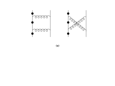
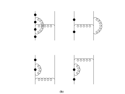
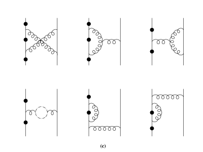
Figure 1: The classes of Feynman diagrams relevant for the different colour structures. The solid circle indicates the possible positions for attaching the off-shell photon to the quark-antiquark pair $i,j$. Group (a) contributes to $A^{(1)}_{A}(i,j)$, (b) to $A^{(1)}_{B}(i,j)$ and group (c) to the leading colour amplitude $A^{(1)}_{C}(i,j)$. Diagrams with self-energy corrections on the external lines are zero in dimensional regularisation and have been omitted.

The squared matrix elements are straightforwardly obtained at leading order [20]. Because the matrix element contracted with the photon momentum vanishes by current conservation, the sum over the polarisations of the gauge boson may be performed in the Feynman gauge,

$$\sum_{\rm spins}\epsilon^{\mu}\epsilon^{*\nu}=-g^{\mu\nu}.$$ (6)

Hence,

$$\sum_{\rm spins}|{\cal M}^{(0)}|^{2}=\frac{e^{2}g_{s}^{4}}{4}(N^{2}-1)$$ (7)

$$\times \Biggl{\{}\biggl{(}{\cal T}(1,2;1,2)+{\cal T}(1,2;3,4)\biggr{)}+\frac{\delta_{qQ}}{N}\biggl{(}{\cal T}(1,2;1,4)+{\cal T}(1,2;3,2)\biggr{)}\Biggr{\}}$$

$$+(1\leftrightarrow 3,2\leftrightarrow 4)+\delta_{qQ}(2\leftrightarrow 4)+\delta_{qQ}(1\leftrightarrow 3),$$

where,

$${\cal T}(i,j;k,l)=\sum_{\rm spins}|A^{(0)\dagger}(i,j){\cal A}^{(0)}(k,l)|.$$ (8)

The relevant ‘squared’ matrix elements are the interference between the tree-level and one-loop amplitudes,

$$\sum_{\rm spins}2|{\cal M}^{(0)\dagger}{\cal M}^{(1)}|=\frac{e^{2}g_{s}^{4}}{4}\left(\frac{\alpha_{s}N}{2\pi}\right)(N^{2}-1)$$ (9)

$$\times \Biggl{\{}\biggl{[}\biggl{(}{\cal L}_{C}(1,2;1,2)+{\cal L}_{C}(1,2;3,4)\biggr{)}$$

$$~{}~{}~{}~{}~{}~{}~{}-\frac{1}{N^{2}}\biggl{(}2{\cal L}_{A}(1,2;1,2)+2{\cal L}_{A}(1,2;3,4)+{\cal L}_{B}(1,2;1,2)+{\cal L}_{B}(1,2;3,4)\biggr{)}\biggr{]}$$

$$+\delta_{qQ}\biggl{[}\frac{1}{N}\biggl{(}{\cal L}_{C}(1,2;1,4)+{\cal L}_{C}(1,2;3,2)-{\cal L}_{A}(1,2;1,4)-{\cal L}_{A}(1,2;3,2)\biggr{)}$$

$$~{}~{}~{}~{}~{}~{}~{}-\frac{1}{N^{3}}\biggl{(}{\cal L}_{A}(1,2;1,4)+{\cal L}_{A}(1,2;3,2)+{\cal L}_{B}(1,2;1,4)+{\cal L}_{B}(1,2;3,2)\biggr{)}\biggr{]}\Biggr{\}}$$

$$+(1\leftrightarrow 3,2\leftrightarrow 4)+\delta_{qQ}(2\leftrightarrow 4)+\delta_{qQ}(1\leftrightarrow 3),$$

with,

$${\cal L}_{\alpha}(i,j;k,l)=\sum_{\rm spins}|A^{(1)\dagger}_{\alpha}(i,j){\cal A}^{(0)}(k,l)|.$$ (10)

Using the symmetry properties of the Feynman diagrams, we find that,

$${\cal L}_{\alpha}(1,2;3,2)={\cal L}_{\alpha}(1,2;1,4)(p_{1}\leftrightarrow p_{2},p_{3}\leftrightarrow p_{4}),$$ (11)

so that the ‘squared’ matrix elements are described by 9 independent ${\cal L}_{\alpha}$.

In computing the ‘square’, the loop momentum $\ell^{\mu}$ always appears as either $\ell^{2}$ or $\ell.p$. We therefore systematically reduce the number of loop momenta appearing in the numerator by simple rewriting,

$$\frac{\ell.p}{\ell^{2}(\ell+p)^{2}}=\frac{(\ell+p)^{2}-\ell^{2}-p^{2}}{2\ell^{2}(\ell+p)^{2}}.$$

The only time that we are unable to do this occurs when the loop momentum is contracted with the ‘wrong’ momentum, i.e., one that does not appear in any of the propagators. For the pentagon diagrams, all momenta are involved in the propagators and we can always rewrite the integral as a combination of box tensor-integrals. Dividing through in this way, we find box (triangle) tensor-integrals with at most three (two) loop momenta in the numerator.

The simplified tensor integrals can now be expressed in terms of scalar integrals using a momentum decomposition. We choose the natural momentum as in [17] rather than the reciprocal momentum basis of [18, 5, 12]. The coefficients of the scalar integrals are obtained by solving systems of linear equations and the usual problem is the occurrence of Gram determinants. Typically, for a rank $n$ tensor $m$-point diagram, we can obtain an $(m-1)\times(m-1)$ Gram determinant raised to the $n$th power in the denominator. Since the physical process does not usually possess singularities near the edge of phase space where the Gram determinants vanish, one obtains large cancellations between terms and potential numerical inaccuracies. For ‘squared’ one-loop matrix elements the number of terms is expected to be large, thereby exacerbating the numerical problem. However, since these Gram determinant singularities are unphysical, it should prove possible to arrange the scalar integrals in combinations that are finite in the limit that the Gram determinant vanishes. The matrix elements, written in terms of these finite combinations, are then obviously finite and numerically stable in the same limits. The explicit results of Bern, Kosower and Dixon [8, 9] and Kunszt, Signer and Trocsanyi [10, 12] for the five-parton one-loop amplitudes already show the introduction of such functions. For example, Bern, Kosower and Dixon introduce the functions

$$L_{0}(r)=\frac{\log(r)}{1-r},~{}~{}~{}~{}~{}~{}~{}~{}L_{1}(r)=\frac{L_{0}(r)+1}{1-r},$$

which are finite as $r\to 1$. Furthermore, the helicity coefficient of these functions is usually rather simple so one might expect that the ‘squared’ matrix element coefficient is not enormous. We have therefore assembled a collection of finite functions relevant to the process at hand [19] and organised the ${\cal L}_{\alpha}$ as a linear combination of these functions where the coefficients are polynomials of the generalised Mandelstam invariants,

$$s_{ij}=(p_{i}+p_{j})^{2},~{}~{}~{}~{}~{}s_{ijk}=(p_{i}+p_{j}+p_{k})^{2},~{}~{}~{}~{}~{}s_{ijkl}=(p_{i}+p_{j}+p_{k}+p_{l})^{2}.$$

As mentioned earlier, these fuctions are natural in the sense that they are obtained by differentiating the scalar integral with respect to the external kinematic parameters or by evaluating the integral in higher dimensions. However, these finite combinations are not linearly independent (unlike the raw scalar integrals), and by explicitly cancelling part of the polynomial coefficient against the Gram determinant it is possible to shift terms from one function to another. Therefore an ambiguity in the presentation of the final answer remains.

As mentioned earlier, we use dimensional regularisation and work in $D=4-2\epsilon$ dimensions. It is straightforward to remove the infrared and ultraviolet singularities poles from the ${\cal L}_{\alpha}$ since they are proportional to the tree-level amplitudes,

$${\cal L}_{A}(1,2;i,j) = \left(+\frac{{\cal P}_{13}}{\epsilon^{2}}-\frac{{\cal P}_{14}}{\epsilon^{2}}-\frac{{\cal P}_{23}}{\epsilon^{2}}+\frac{{\cal P}_{24}}{\epsilon^{2}}\right){\cal T}(1,2;i,j)+\hat{\cal L}_{A}(1,2;i,j),$$ (12)

$${\cal L}_{B}(1,2;i,j) = \left(-\frac{{\cal P}_{12}}{\epsilon^{2}}-\frac{{\cal P}_{34}}{\epsilon^{2}}-\frac{3{\cal P}_{34}}{\epsilon}\right){\cal T}(1,2;i,j)+\hat{\cal L}_{B}(1,2;i,j),$$ (13)

$${\cal L}_{C}(1,2;i,j) = \left(-\frac{{\cal P}_{14}}{\epsilon^{2}}-\frac{{\cal P}_{23}}{\epsilon^{2}}+\frac{2}{3}\frac{{\cal P}_{34}}{\epsilon}-\frac{2N_{F}}{3N}\frac{{\cal P}_{34}}{\epsilon}\right){\cal T}(1,2;i,j)+\hat{\cal L}_{C}(1,2;i,j),$$ (14)

where we have introduced the notation,

$${\cal P}_{ij}=\left(\frac{4\pi\mu^{2}}{-s_{ij}}\right)^{\epsilon}\frac{\Gamma^{2}(1-\epsilon)\Gamma(1+\epsilon)}{\Gamma(1-2\epsilon)}.$$ (15)

In physical cross sections, this pole structure must cancel with the infrared poles from the $\gamma^{*}\to q\bar{q}Q\bar{Q}+g$ process and those generated by ultraviolet renormalisation. This pole structure is in agreement with the expectations of ref. [21] and reproduces that given in [11, 12].

The finite functions $\hat{\cal L}$ can be written in the following symbolic way,

$$\hat{\cal L}=\sum_{i}P_{i}(s){\rm L}_{i},$$ (16)

where $P_{i}(s)$ is a polynomial of the invariant masses $s_{ij}$ and the ${\rm L}_{i}$ are linear combinations of scalar loop integrals. Rather than have the Gram determinants present in the polynomial coefficients as in the conventional method [17, 18, 5, 12]), they are absorbed into the ${\rm L}_{i}$ which are constructed to be well behaved in the limit that the Gram determinant vanishes. The advantage is better numerical stability while the disadvantage is that there are rather more functions (than the raw scalar integrals in $4-2\epsilon$ dimensions). Furthermore, since the functions are not linearly independent the polynomial coefficients are not unique. Typically, the $P_{i}(s)$ contains ${\cal O}(30)$ terms (roughly the same size as the tree level result) while the summation runs over ${\cal O}(30)$ functions. Although the expreassions for the individual $\hat{\cal L}_{\alpha}$ are in closed form, they are still rather lengthy and each contains several hundred terms. We have therefore constructed a FORTRAN subroutine detailing the $P_{i}(s)$ and evaluating the finite one-loop contribution for a given phase space point. This will act as an ingredient in calculating the full next-to-leading order $e^{+}e^{-}\to 4$ jet rate once the necessary sub-leading colour contributions to the $\gamma^{*}\to q\bar{q}gg$ matrix elements are known via numerical combination with the tree level $\gamma^{*}\to 5$ parton processes [22, 23, 24].

To illustrate the finite groupings ${\rm L}_{i}$ and the potential numerical instabilities, we show the functions associated with the triangle graph with three massive external legs. The scalar triangle integral with momenta $p_{12}$ and $p_{34}$ flowing out (and $p_{1234}$ flowing in) can be written [25, 5],

$${\rm Lc}_{0}(p_{12},p_{34})=\frac{1}{\sqrt{-\Delta_{3}}}\left(\log(a^{+}a^{-})\log\left(\frac{1-a^{+}}{1-a^{-}}\right)+2{\rm Li_{2}}(a^{+})-2{\rm Li_{2}}(a^{-})\right),$$ (17)

where ${\rm Li_{2}}$ is the usual dilogarithm function and $a^{\pm}$ are two roots of a quadratic equation,

$$a^{\pm}=\frac{s_{1234}+s_{34}-s_{12}\pm\sqrt{-\Delta_{3}}}{2s_{1234}},$$ (18)

and,

$$\Delta_{3}=-s_{1234}^{2}-s_{12}^{2}-s_{34}^{2}+2s_{1234}s_{12}+2s_{1234}s_{34}+2s_{12}s_{34}.$$ (19)

The functions,

$${\rm Lc}_{1S}(p_{12},p_{34}) = \frac{1}{2\Delta_{3}}\Biggl{(}2s_{1234}s_{12}s_{34}{\rm Lc}_{0}(p_{12},p_{34})$$

$$-\left(s_{12}(s_{1234}+s_{34}-s_{12})\log\left(\frac{s_{1234}}{s_{12}}\right)+s_{34}(s_{1234}+s_{12}-s_{34})\log\left(\frac{s_{1234}}{s_{34}}\right)\right)\Biggr{)},$$

$${\rm Lc}_{2S}(p_{12},p_{34}) = \frac{1}{4\Delta_{3}}\Biggl{(}2s_{1234}s_{12}s_{34}{\rm Lc}_{1S}(p_{12},p_{34})-\frac{1}{3}s_{1234}s_{12}s_{34}$$

$$-\frac{1}{6}\left(s_{12}^{2}(s_{1234}+s_{34}-s_{12})\log\left(\frac{s_{1234}}{s_{12}}\right)+s_{34}^{2}(s_{1234}+s_{12}-s_{34})\log\left(\frac{s_{1234}}{s_{34}}\right)\right)\Biggr{)},$$

also appear and are related to the scalar triangle integral in $D=6-2\epsilon$ and $D=8-2\epsilon$ dimensions [19]. Throughout, the arguments of the functions describe the momenta flowing out of all but one of the vertices, while the final momentum is determined by momentum conservation. For triangle integrals it is also convenient to introduce the additional functions corresponding to integrals in $4-2\epsilon$ dimensions with Feynman parameters in the numerator [19], for example,

$${\rm Lc}_{1}(p_{12},p_{34}) = \frac{1}{\Delta_{3}}\Biggl{(}s_{12}(s_{1234}-s_{12}+s_{34}){\rm Lc}_{0}(p_{12},p_{34})$$ (22)

$$-(s_{1234}-s_{12}-s_{34})\log\left(\frac{s_{1234}}{s_{34}}\right)-2s_{12}\log\left(\frac{s_{1234}}{s_{12}}\right)\Biggr{)},$$

$${\rm Lc}_{2}(p_{12},p_{34}) = \frac{1}{2\Delta_{3}}\Biggl{(}2s_{34}(s_{1234}+s_{12}-s_{34}){\rm Lc}_{1}(p_{12},p_{34})+s_{12}(s_{1234}+s_{34}-s_{12}){\rm Lc}_{1}(p_{34},p_{12})$$ (23)

$$\qquad\qquad-s_{12}s_{34}{\rm Lc}_{0}(p_{12},p_{34})-s_{34}\log\left(\frac{s_{1234}}{s_{34}}\right)+s_{12}+s_{34}-s_{1234}\Biggr{)}.$$

As $\Delta_{3}\to 0$, all of these functions are finite and combine dilogarithms and logarithms in a highly non-trivial way. For example,

$$\lim_{\Delta_{3}\to 0}{\rm Lc}_{1S}(p_{12},p_{34}) = \frac{1}{12s_{12}s_{34}s_{1234}}\Biggl{(}s_{12}^{2}(s_{1234}+s_{34}-s_{12})\log\left(\frac{s_{1234}}{s_{12}}\right)$$ (24)

$$\qquad+s_{34}^{2}(s_{1234}+s_{12}-s_{34})\log\left(\frac{s_{1234}}{s_{34}}\right)+2s_{12}s_{34}s_{1234}\Biggr{)}.$$

By keeping terms proportional to $\Delta_{3}$ (and higher), the limit can be approached with arbitrary precision.

Numerically, the instability due to the Gram determinant is easy to see if we restrict ourselves to a specific phase space point, $s_{1234}=1,~{}~{}s_{12}=0.2$ and letting $s_{34}$ vary in such a way that $\Delta_{3}\to 0$. This corresponds to $s_{34}\to 0.135$ which is neither the soft nor collinear limit and there should be no kinematic singularity. The behaviour of the various triangle functions is illustrated in Fig. 2 as a function of $\Delta_{3}/\Delta_{3}^{{\rm max}}$ where $\Delta_{3}^{{\rm max}}=-(s_{1234}-s_{12})^{2}$ For a given numerical precision, $acc$, the numerical problems typically occur when $\Delta_{3}/\Delta_{3}^{{\rm max}}\sim(acc)^{1/N}$ where $N$ is the number of Gram determinants in the denominator of the function. Since the scalar integral already contains $\Delta_{3}^{-1/2}$, for an intrinsic numerical precision of roughly $10^{-14}$, the ${\rm Lc}_{1}$ and ${\rm Lc}_{1S}$ functions break down at $\Delta_{3}/\Delta_{3}^{{\rm max}}\sim{\rm few~{}}\times 10^{-10}$ while the ${\rm Lc}_{2}$ and ${\rm Lc}_{2S}$ functions with effectively $2.5$ inverse powers of $\Delta_{3}$ break down at $\Delta_{3}/\Delta_{3}^{{\rm max}}\sim{\rm few~{}}\times 10^{-6}$. Other phase space points yield a similar behaviour. With adaptive Monte Carlo methods such as VEGAS [26], once the singular region is found, more and more Monte Carlo points are generated there and the result will be unreliable. However, for $\Delta_{3}<10^{-5}\Delta_{3}^{{\rm max}}$ we see that the approximate form obtained by making a Taylor expansion about $\Delta_{3}=0$ and keeping only the constant term works well.

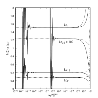
Figure 2: The finite functions for the triply massive triangle graph with $s_{1234}=1$ and $s_{12}=0.2$ as a function of $\Delta_{3}/\Delta_{3}^{{\rm max}}$ where $\Delta_{3}^{{\rm max}}=-(s_{1234}-s_{12})^{2}$. The dashed lines show the approximate form for the function in the limit $\Delta_{3}\to 0$, retaining only the first term of the Taylor expansion.

Similar groupings for the box and pentagon graphs (with their corresponding Gram determinants) can be obtained by considering the scalar integrals in higher dimensions or with Feynman parameters in the numerator [19]. This approach is easily generalisable to other processes with more general kinematics.

To summarize, we have performed the first calculation of the one-loop ‘squared’ matrix elements for the $\gamma^{*}\to q\bar{q}Q\bar{Q}$ process keeping all orders in the number of colours. Throughout conventional dimensional regularisation has been employed as well as grouping the Feynman diagrams according to the colour structure. However, in order to deal with the Gram determinants, we have expressed the formfactors in terms of functions (${\rm L}_{i}$) which group together dilogarithms, logarithms and constants from the basic scalar integrals in a way that is well behaved as the Gram determinants vanish. These groupings are derived by differentiating the scalar integrals with respect to the external kinematic factors or by considering them in higher dimensions. The resulting expressions are still rather long, due partly to the number of functions and partly to the size of the tree-level matrix elements, but numerically stable and ready to be implemented in next-to-leading order Monte Carlo calculations of the $e^{+}e^{-}\to 4~{}{\rm jet}$, $e^{\pm}p\to e^{\pm}+3~{}{\rm jet}$ and $p\bar{p}\to V+2~{}{\rm jet}$ processes.

Acknowledgements

We thank Walter Giele, Eran Yehudai, Bas Tausk and Keith Ellis for collaboration in the earlier stages of this work and John Campbell for numerous comments and suggestions in the latter stages. DJM thanks the UK Particle Physics and Astronomy Research Council for the award of a research studentship.

References

- [1] see for example, Z. Bern, L. Dixon and D. A. Kosower, ‘Progress in one loop QCD computations’, submitted to Ann. Rev. Nucl. Part. Sci., hep-ph/9602280.
- [2] W. L. van Neerven and J. A. M. Vermaseren, Phys. Letts. B137 (1984) 241.
- [3] Z. Bern, L. Dixon and D. A. Kosower, Nucl. Phys. B412 (1994) 751.
- [4] Z. Bern, L. Dixon and D. A. Kosower, Phys. Lett. B302 (1993) 299, ibid B318 (1993) 649.
- [5] R. K. Ellis, W. T. Giele and E. Yehudai, private communication.
- [6] Z. Kunszt, A. Signer and Z. Trocsanyi, Nucl. Phys. B411 (1994) 397.
- [7] S. Catani, M. H. Seymour and Z. Trocsanyi, ‘Regularization Scheme Independence and Unitarity in QCD Cross Sections’, hep-ph/9610553.
- [8] Z. Bern, L. Dixon and D. A. Kosower, Phys. Rev. Lett. 70 (1993) 2677.
- [9] Z. Bern, L. Dixon and D. A. Kosower, Nucl. Phys. B437 (1995) 259.
- [10] Z. Kunszt, A. Signer and Z. Trocsanyi, Phys. Lett. B336 (1994) 529.
- [11] A. Signer, Phys. Letts. B357 (1995) 204.
- [12] A. Signer, Ph.D. thesis, ‘Helicity method for next-to-leading order corrections in QCD’, ETH Zurich (1995).
- [13] Z. Bern, L. Dixon and D. A. Kosower, ‘Unitarity based techniques for one loop calculations in QCD’, hep-ph/9606378.
- [14] L. Dixon and A. Signer, ‘Electron-Positron Annihilation into Four Jets at Next-to-Leading Order in ’, SLAC preprint SLAC-PUB-7309, hep-ph/9609460.
- [15] Z. Bern, L. Dixon, D. A. Kosower and S. Wienzierl, ‘One-Loop Amplitudes for ’, hep-ph/9610370.
- [16] G. ’t Hooft and M. Veltman, Nucl. Phys. B44 (1972) 189.
-
[17]
L. M. Brown and R. P. Feynman,
Phys. Rev. 85 (1952) 231;
G. Passarino and M. Veltman, Nucl. Phys. B160 (1979) 151. - [18] G.J. van Oldenborgh and J.A.M. Vermaseren, Z. Phys. C46 (1990) 425.
- [19] J. M. Campbell, E. .W. N. Glover and D. J. Miller, ‘One-Loop Tensor Integrals in Dimensional Regularisation’, hep-ph/9612413.
- [20] R. K. Ellis, D. A. Ross and A. E. Terrano, Nucl. Phys. B178 (1981) 421.
- [21] W. T. Giele and E. W. N. Glover, Phys. Rev. D46 (1992) 1980.
- [22] K. Hagiwara and D. Zeppenfeld, Nucl. Phys. B313 (1989) 560.
- [23] F. A. Berends, W. T. Giele and H. Kuijf, Nucl. Phys. B321 (1989) 39.
- [24] N. K. Falk, D. Graudenz and G. Kramer, Nucl. Phys. B328 (1989) 317.
-
[25]
D. Kreimer, Int. J. Mod. Phys. A8 (1993) 1797;
A. Davydychev, J. Phys. A25 (1992) 5587. - [26] G. P. Lepage, J. Comp. Phys. 27 (1978) 192.