DESY 96-202
hep-ph/9609445

Instantons in Deep–Inelastic Scattering
– The Simplest Process –

Instanton calculations in QCD are generically plagued by infrared divergencies associated with the integration over the instanton size $\rho$. Here, we demonstrate explicitly that the typical inverse hard momentum scale ${\mathcal{Q}}^{-1}$ in deep-inelastic scattering provides a dynamical infrared cutoff for the size parameter $\rho$. Hence, deep-inelastic scattering may be viewed as a distinguished process for studying manifestations of QCD-instantons. For clarity, we restrict the explicit discussion to the simplest chirality-violating process, $\gamma^{\ast}+{\rm g}\rightarrow\overline{{\rm q}_{L}}+{\rm q}_{R}\,$. We calculate the corresponding fixed angle cross-section as well as the contributions to the gluon structure functions, ${\mathcal{F}}_{2\,g}$ and ${\mathcal{F}}_{L\,g}$, within standard instanton perturbation theory in leading semi-classical approximation. To this approximation, fixed-angle scattering processes at high $Q^{2}$ are reliably calculable. In the Bjorken limit, the considered instanton-induced process gives a scaling contribution to ${\mathcal{F}}_{2\,g}(x,Q^{2})$ and the Callan-Gross relation holds.

1 Introduction

Instantons [1] are well known to represent tunnelling transitions in non-abelian gauge theories between degenerate vacua of different topology. These transitions induce processes which are forbidden in perturbation theory, but have to exist in general [2] due to Adler-Bell-Jackiw anomalies. Correspondingly, these processes imply a violation of certain fermionic quantum numbers, notably, $B+L$ in the electro-weak gauge theory and chirality ($Q_{5}$) in (massless) QCD.

An experimental discovery of such a novel, non-perturbative manifestation of non-abelian gauge theories would clearly be of basic significance.

A number of results has revived the interest in instanton-induced processes during recent years:

• First of all, it was shown [3, 4] that the generic exponential suppression of these tunnelling rates, $\propto\exp(-4\pi/\alpha)$, may be overcome at high energies, mainly due to multi-gauge boson emission in addition to the minimally required fermionic final state.

• A pioneering and encouraging theoretical estimate of the size of the instanton ($I$) induced contribution to the gluon structure functions in deep-inelastic scattering was recently presented in Ref. [5]. The summation over the $I$-induced multi-particle final state was implicitly performed by starting from the optical theorem for the virtual $\gamma^{\ast}g\rightarrow\gamma^{\ast}g$ forward amplitude. The strategy was then to evaluate the contribution to the functional integral coming from the vicinity of the instanton-antiinstanton ($I\overline{I}$) configuration in Euclidean space, to analytically continue the result to Minkowski space and, finally, to take the imaginary part. While the instanton-induced contribution to the gluon structure functions turned out to be small at larger values of the Bjorken variable $x$, it was found in Ref. [5] to increase dramatically towards smaller $x$.

• Last not least, a systematic phenomenological and theoretical study is under way [6, 7, 8, 9], which clearly indicates that deep-inelastic $ep$ scattering at HERA now offers a unique window to experimentally detect QCD-instanton induced processes through their characteristic final-state signature. The searches for instanton-induced events have just started at HERA and a first upper limit of $0.9$ nb at $95\%$ confidence level for the cross-section of QCD-instanton induced events has been placed by the H1 Collaboration [10]. New, improved search strategies are being developped [9] with the help of a Monte Carlo generator (QCDINS 1.3) [7] for instanton-induced events.

The central question is, of course, whether instanton-induced processes in deep-inelastic scattering can both be reliably computed and experimentally measured. In particular, whether contributions associated with the non-perturbative vacuum structure can be controlled in the same way as perturbative short-distance corrections, in terms of a hard scale ${\mathcal{Q}}$.

In the work of Refs. [5, 11] on deep-inelastic scattering, the integrals over the instanton size $\rho$ were found to be infrared (IR) divergent, like in a number of previous instanton calculations in different areas. Yet, the authors claimed that this problem does not affect the possibility, to isolate in deep-inelastic scattering a well-defined, IR-finite and sizable instanton contribution in the regime of small QCD-gauge coupling, on account of the (large) photon virtuality $Q^{2}$. The IR-divergent pieces of the $I$-size integrals were supposed to be factorizable into the parton distributions, which anyway have to be extracted from experiment at some reference scale.

On the other hand, also IR-finite instanton contributions to certain observables in momentum space have been found in the past [12, 13]. In this ideal case, the size of the contributing instantons is limited by the inverse momentum scale ${\mathcal{Q}}^{-1}$ of the experimental probe, as one might intuitively expect. No ad hoc cutoff or assumption about the behaviour of large, overlapping instantons need be introduced.

A main issue of the present work is to shed further light on these important questions around the IR-behaviour associated with the instanton size in deep-inelastic scattering. This paper represents the first of several papers in preparation [14], containing our theoretical results on $I$-induced processes in the deep-inelastic regime.

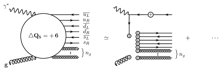
Figure 1: Instanton-induced chirality-violating process,
$\gamma^{\ast}+{\rm g}\rightarrow\sum_{\rm flavours}^{n_{f}}\left[\overline{{\rm q}_{L}}+{\rm q}_{R}\right]+n_{g}\,{\rm g}$, corresponding to three massless flavours ($n_{f}=3$).

For clarity, let us reduce here the realistic task of evaluating the $I$-induced cross-sections of the chirality violating multi-particle processes (illustrated in Fig. 1)

$$\gamma^{\ast}+{\rm g}\Rightarrow\overline{{\rm u}_{L}}+{\rm u}_{R}\,+\overline{{\rm d}_{L}}+{\rm d}_{R}\,+\overline{{\rm s}_{L}}+{\rm s}_{R}\,+n_{g}\,{\rm g},$$ (1)

to the detailed study of the simplest one, without additional gluons and with just one massless flavour ($n_{f}=1$),

$$\gamma^{\ast}(q)+{\rm g}(p)\Rightarrow\overline{{\rm q}_{L}}(k_{1})+{\rm q}_{R}(k_{2})\,.$$ (2)

The price is, of course, that this process only represents a small fraction of the total $I$-induced contribution to the gluon structure functions.

However, there are also a number of important virtues:

The present calculation provides a clean and explicit discussion of most of the crucial steps involved in our subsequent task [14] to calculate the dominant $I$-induced contributions. While unessential technical complications have been eliminated here, a generalization to the realistic case with gluons and more flavours in the final state is entirely straightforward [14, 15]. We shall explicitly calculate the corresponding fixed angle cross-section and the contributions to the gluon structure functions in leading semi-classical approximation within standard instanton perturbation theory (Sect. 3). Gauge invariance is kept manifest along the calculation and we may compare at various stages with the appropriate chirality-conserving process, calculated in leading order of perturbative QCD.

As a central result of this paper and unlike Ref. [5], we find no IR divergencies associated with the integration over the instanton size $\rho$, which can even be perfomed analytically. We are able to demonstrate explicitly that the typical hard scale ${\mathcal{Q}}$ in deep-inelastic scattering provides a dynamical infrared cutoff for the instanton size, $\rho\mbox{\,\raisebox{1.29167pt}{$<$}$\!\!\!\!\!$\raisebox{-3.87495pt}{$\sim$}\,}{\mathcal{O}}(1/{\mathcal{Q}})$. Additional gluons in the final state will not change this conclusion, as is briefly outlined in Sect. 4. Thus, deep-inelastic scattering may indeed be viewed as a distinguished process for studying manifestations of QCD-instantons.

2 Setting the Stage

Let us start with the matrix elements ${\mathcal{T}}^{\mu}(q,p;k_{1},\ldots,k_{n})$ of the general, exclusive photon-parton reactions

$$\gamma^{\ast}(q)+p\rightarrow k_{1}+\ldots+k_{n}\,,$$ (3)

in terms of which we form the inclusive structure tensor ${\mathcal{W}}^{\mu\nu}_{p}$ of the parton $p$,

$${\mathcal{W}}^{\mu\nu}_{p}(q,p) = \sum_{n=1}^{\infty}{\mathcal{W}}^{\mu\nu\,(n)}_{p}(q,p)\,,\hskip 24.0pt{\rm with}$$ (4)

$${\mathcal{W}}^{\mu\nu(n)}_{p}(q,p) = \frac{1}{4\,\pi}\,\int dPS^{(n)}\,{\mathcal{T}}^{\mu}(q,p;k_{1},\ldots,k_{n}){\mathcal{T}}^{\nu\,\ast}(q,p;k_{1},\ldots,k_{n}),$$ (5)

and

$$\int dPS^{(n)}=\prod_{j=1}^{n}\int\frac{d^{4}k_{j}}{(2\,\pi)^{3}}\,\delta^{(+)}\left(k_{j}^{2}\right)(2\,\pi)^{4}\,\delta^{(4)}\left(q+p-k_{1}-\ldots-k_{n}\right)\,.$$ (6)

Averaging over colour and spin of the initial state is implicitly understood in Eq. (5); the index $n$ is to label besides the final state partons also their spin and colour degrees of freedom.

For exclusive $2\rightarrow 2$ processes, $\gamma^{\ast}(q)+p\rightarrow k_{1}+k_{2}$, the differential cross-section is then expressed as

$$\frac{d\sigma}{dt}=8\,\pi^{2}\,\alpha\ \frac{x}{Q^{2}}\,\left[-g_{\mu\nu}\,\frac{d{\mathcal{W}}^{\mu\nu\,(2)}_{p}}{dt}\right]\,,$$ (7)

where $Q^{2}=-q^{2}$ denotes the photon virtuality and

$$t=\left(q-k_{1}\right)^{2}=\left(p-k_{2}\right)^{2}\,,$$ (8)

the momentum transfer squared.

In general, each final state, $k_{1}+\ldots+k_{n}$, contributes to the structure functions ${\mathcal{F}}_{i\,{p}}$ of the parton $p$ via the projections

$${\mathcal{F}}^{(n)}_{2\,{p}}(x,Q^{2}) = \left[-g_{\nu\mu}\,+6\,x\,\frac{p_{\mu}p_{\nu}}{p\cdot q}\right]x\,{\mathcal{W}}_{p}^{\mu\nu\,(n)}(q,p)\,,$$ (9)

$${\mathcal{F}}^{(n)}_{L\,{p}}(x,Q^{2}) = 4\,x^{2}\,\frac{p_{\mu}p_{\nu}}{p\cdot q}{\mathcal{W}}_{p}^{\mu\nu\,(n)}(q,p)\ ,\hskip 24.0pt{\rm such\ that}$$ (10)

$${\mathcal{F}}_{i\,{p}}(x,Q^{2}) = \sum_{n=1}^{\infty}{\mathcal{F}}^{(n)}_{i\,{p}}(x,Q^{2})\,,$$ (11)

with

$$x\equiv\frac{Q^{2}}{2\,p\cdot q}\,.$$ (12)

denoting the Bjorken variable of the photon-parton subprocess.

The spin averaged proton structure functions $F_{2}$ and $F_{L}$, appearing (in the one photon exchange approximation) in the unpolarized inclusive lepto-production cross-section as

$$\frac{d^{2}\sigma}{dx_{\rm Bj}\,dy_{\rm Bj}}=\frac{4\pi\alpha^{2}}{Sx_{\rm Bj}^{2}y_{\rm Bj}^{2}}\left[\left\{1-y_{\rm Bj}+\frac{y_{\rm Bj}^{2}}{2}\right\}F_{2}(x_{\rm Bj},Q^{2})-\frac{y_{\rm Bj}^{2}}{2}F_{L}(x_{\rm Bj},Q^{2})\right],$$ (13)

are expressed via a standard convolution in terms of the parton structure functions ${\mathcal{F}}_{i\,{p}}$ and corresponding parton densities $f_{p}$,

$$F_{i}\,(x_{\rm Bj},Q^{2})=\sum_{p=q,g}\int_{x_{\rm Bj}}^{1}\frac{dx}{x}\,f_{p}\left(\frac{x_{\rm Bj}}{x}\right)\,\frac{x_{\rm Bj}}{x}\,{\mathcal{F}}_{i\,{p}}(x,Q^{2})\ ,\ \ i=2,L\,.$$ (14)

Here, $\sqrt{S}$ is the center-of-mass (c.m.) energy of the lepton-hadron system. The corresponding Bjorken variables are defined as usual

$$x_{\rm Bj}\equiv\frac{Q^{2}}{2\,P\cdot q};\hskip 48.0pty_{\rm Bj}\equiv\frac{P\cdot q}{P\cdot k},$$ (15)

where $P\,(k)$ is the four-momentum of the incoming proton (lepton).

Figure 2: Perturbative chirality-conserving process, $\gamma^{\ast}(q)+{\rm g}(p)\rightarrow\overline{{\rm q}_{L}}(k_{1})+{\rm q}_{L}(k_{2})$.

As outlined in the Introduction, we shall consider in this paper only the contributions from the simplest instanton-induced, chirality-violating photon-gluon process, corresponding to one massless quark flavour $(n_{f}=1)$,

$$\gamma^{\ast}(q)+{\rm g}(p)\rightarrow\overline{{\rm q}_{L}}(k_{1})+{\rm q}_{R}(k_{2})\ ;\hskip 24.0pt\left(\triangle Q_{5}\equiv\triangle\left(Q_{R}-Q_{L}\right)=2\right)\,.$$ (16)

It will be very instructive to compare with the appropriate leading-order perturbative QCD amplitudes for the chirality-conserving process (Fig. 2),

$$\gamma^{\ast}(q)+{\rm g}(p)\rightarrow\overline{{\rm q}_{L}}(k_{1})+{\rm q}_{L}(k_{2})\ ;\hskip 24.0pt\left(\triangle Q_{5}\equiv\triangle\left(Q_{R}-Q_{L}\right)=0\right)\,.$$ (17)

at the various stages of the instanton calculation. Therefore, for reference, let us summarize the well-known perturbative results next (see any textbook on perturbative QCD, e.g. Ref. [16]).

Let us use two-component Weyl-notation for the (massless) fermions involved, in order to facilitate the comparison with the instanton calculation later on. The leading-order amplitude for the perturbative process (17) (Fig. 2) then reads,

$${\mathcal{T}}^{A}_{\mu\,\mu^{\prime}}\left(\gamma^{\ast}+{\rm g}\rightarrow\overline{{\rm q}_{L}}+{\rm q}_{L}\right)=$$

$$e_{q}\,g_{s}\,t^{A}\,\chi_{L}^{\dagger}(k_{2})\left[\overline{\sigma}_{\mu^{\prime}}\frac{(q-k_{1})}{(q-k_{1})^{2}}\overline{\sigma}_{\mu}-\overline{\sigma}_{\mu}\frac{(q-k_{2})}{(q-k_{2})^{2}}\overline{\sigma}_{\mu^{\prime}}\right]\chi_{L}(k_{1})\ ,$$

where the two-component Weyl-spinors $\chi_{L,\,R}$ satisfy the Weyl-equations,

$$\overline{k}\,\chi_{L}(k)=0\,;\hskip 24.0ptk\,\chi_{R}(k)=0\,,$$ (19)

and

$$\chi_{L}(k)\,\chi_{L}^{\dagger}(k)=k\,;\hskip 24.0pt\chi_{R}(k)\,\chi_{R}^{\dagger}(k)=\overline{k}\,.$$ (20)

In Eqs. (2-20) and throughout the paper we use the abbreviations,

$$v\equiv v_{\mu}\,\sigma^{\mu}\,;\hskip 24.0pt\overline{v}\equiv v_{\mu}\,\overline{\sigma}^{\mu}\,,\ \mbox{for any four-vector $v_{\mu}$},$$ (21)

where the familiar $\sigma$-matrices satisfy,

$$\sigma_{\mu}\overline{\sigma}_{\nu}+\sigma_{\nu}\overline{\sigma}_{\mu}=2\,g_{\mu\nu}\,.$$ (22)

Finally, in Eq. (2), $t^{A},A=1,\ldots,8$, are the SU(3) generators, $e_{q}$ is the quark charge in units of the electric charge $e$, and $g_{s}$ is the SU(3) gauge coupling.

With help of Eqs. (19), (22) and the on-shell conditions $k_{1}^{2}=k_{2}^{2}=0$, the gauge-invariance constraints,

$$q^{\mu}\,{\mathcal{T}}^{A}_{\mu\,\mu^{\prime}}=0\,;\hskip 24.0pt{\mathcal{T}}^{A}_{\mu\,\mu^{\prime}}\,p^{\mu^{\prime}}=0\,,$$ (23)

are easily checked.

Next, we obtain the leading-order contribution of the process (17) to ${\mathcal{W}}^{\mu\nu\,(2)}_{g}(q,p)$ by contracting Eq. (2) with the gluon polarization vector $\epsilon_{g}^{\mu^{\prime}}(p)$ and taking the traces in Eq. (5) by means of relations (20) and (22). Averaging over the initial-state gluon polarization and colour amounts to an overall factor $1/16$. The final result for the projections needed in Eqs. (7), (9), and (10) then reads

$$-g_{\mu\nu}\,\frac{d{\mathcal{W}}^{\mu\nu\,{(2)}}_{g}}{dt}\,\left(\gamma^{\ast}+{\rm g}\rightarrow\overline{{\rm q}_{L}}+{\rm q}_{L}\right)=$$

$$e_{q}^{2}\,\frac{\alpha_{s}}{4\,\pi}\,\frac{x}{2\,Q^{2}}\,\left[\frac{u}{t}+\frac{t}{u}-2\,\frac{1-x}{x}\,\frac{Q^{4}}{tu}\right]\,,$$

$$\frac{p_{\mu}\,p_{\nu}}{p\cdot q}\,\frac{d{\mathcal{W}}^{\mu\nu\,{(2)}}_{g}}{dt}\,\left(\gamma^{\ast}+{\rm g}\rightarrow\overline{{\rm q}_{L}}+{\rm q}_{L}\right)=e_{q}^{2}\,\frac{\alpha_{s}}{4\,\pi}\,\frac{x\,(1-x)}{Q^{2}}\,,$$ (25)

where $u=-t-Q^{2}/x$.

Upon integrating Eq. (2) over $t$, we encounter the familiar collinear divergencies for $t,u\rightarrow 0$. In order to isolate the hard contributions to the gluon structure functions, it is adequate to regularize the collinear singularities by introducing an infrared cutoff scale $\mu_{c}$ in the integration limits, $\{-Q^{2}/x+\mu_{c}^{2},-\mu_{c}^{2}\}$. On account of Eqs. (9), (10), one then obtains the familiar results in the Bjorken limit,

$${\mathcal{F}}_{2\,g}^{(\overline{{\rm q}_{L}}{\rm q}_{L})}\,(x,Q^{2};\mu_{c}^{2})=e_{q}^{2}\,\frac{\alpha_{s}}{2\,\pi}\,\times$$ (26)

$$x\,\left[P_{qg}(x)\,\ln\left(\frac{Q^{2}}{\mu_{c}^{2}}\right)+P_{qg}(x)\,\ln\left(\frac{1}{x}\right)-\frac{1}{2}+3\,x\,(1-x)\right]\left[1+{\mathcal{O}}\left(\frac{\mu_{c}^{2}}{Q^{2}}\right)\right]\,,$$

$${\mathcal{F}}_{L\,g}^{(\overline{{\rm q}_{L}}{\rm q}_{L})}\,(x,Q^{2})=e_{q}^{2}\,\frac{\alpha_{s}}{\pi}\,x^{2}\,(1-x)\,,$$ (27)

with the splitting function

$$P_{qg}(x)\equiv\frac{1}{2}\,\left(x^{2}+(1-x)^{2}\right)\,.$$ (28)

Of course, the finite part of the structure function ${\mathcal{F}}_{2\,g}^{(\overline{{\rm q}_{L}}{\rm q}_{L})}$, that is everything except for the large logarithm, $\ln(Q^{2}/\mu_{c}^{2})$, is scheme dependent.

3 The Instanton-Induced Process
$\gamma^{\ast}+{\rm g}\rightarrow\overline{{\rm q}_{L}}+{\rm q}_{R}$

In this section, we turn to the central issue of this paper. We consider the simplest instanton-induced exclusive process, $\gamma^{\ast}+{\rm g}\rightarrow\overline{{\rm q}_{L}}+{\rm q}_{R}$, and compute its contributions to the fixed angle differential cross-section and the gluon structure functions ${\mathcal{F}}_{2\,{g}}$ and ${\mathcal{F}}_{L\,{g}}$, in leading semi-classical approximation.

To this end, the respective Green’s function is first set up according to standard instanton-perturbation theory in Euclidean configuration space [2, 17, 18, 19, 3], then Fourier transformed to momentum space, LSZ amputated, and finally continued to Minkowski space.

The basic building blocks are (in Euclidean configuration space and in the singular gauge):

i) The classical instanton gauge field [1] $A^{(I)}_{\mu^{\prime}}$,

$$A_{\mu^{\prime}}^{(I)}(x) = -{\rm i}\,\frac{2\,\pi^{2}}{g_{s}}\,\rho^{2}\,U\,\left(\frac{\sigma_{\mu^{\prime}}\,\overline{x}-x_{\mu^{\prime}}}{2\,\pi^{2}\,x^{4}}\right)\,U^{\dagger}\ \frac{1}{\Pi_{x}}\,,$$ (29)

$$\Pi_{x} \equiv 1+\frac{\rho^{2}}{x^{2}}\,,$$ (30)

depending on the various collective coordinates, the instanton size $\rho$ and the colour orientation matrices $U^{k}_{\ \alpha}$. The $U$ matrices involve both colour ($k=1,2$) and spinor ($\alpha=1,2$) indices, the former ranging as usual only in the $2\times 2$ upper left corner of $3\times 3$ SU(3) colour matrices. Indices will, however, be suppressed, as long as no confusion can arise.

ii) The quark zero modes [2], $\kappa$ and $\overline{\phi}$,

$$\kappa^{m}_{\ \dot{\beta}}\,(x) = 2\,\pi\,\rho^{3/2}\,\epsilon^{\gamma\delta}\,\left(U\right)^{m}_{\ \delta}\,\frac{\overline{x}_{\dot{\beta}\gamma}}{2\,\pi^{2}\,x^{4}}\ \frac{1}{\Pi_{x}^{3/2}}\,,$$ (31)

$$\overline{\phi}^{\dot{\alpha}}_{\ l}\,(x) = 2\,\pi\,\rho^{3/2}\,\epsilon_{\gamma\delta}\,\left(U^{\dagger}\right)^{\gamma}_{\ l}\,\frac{x^{\delta\dot{\alpha}}}{2\,\pi^{2}\,x^{4}}\ \frac{1}{\Pi_{x}^{3/2}}\,,$$ (32)

and

iii) the quark propagators in the instanton background [17],

$$S^{(I)}(x,y)=$$ (33)

$$\frac{1}{\sqrt{\Pi_{x}\Pi_{y}}}\left[\frac{x-y}{2\pi^{2}(x-y)^{4}}\left(1+\rho^{2}\frac{\left[Ux\overline{y}U^{\dagger}\right]}{x^{2}y^{2}}\right)+\frac{\rho^{2}\sigma_{\mu}}{4\pi^{2}}\frac{\left[Ux\,(\overline{x}-\overline{y})\sigma_{\mu}\overline{y}U^{\dagger}\right]}{x^{2}(x-y)^{2}y^{4}\Pi_{y}}\right],$$

$$\overline{S}^{(I)}(x,y)=$$ (34)

$$\frac{1}{\sqrt{\Pi_{x}\Pi_{y}}}\left[\frac{\overline{x}-\overline{y}}{2\pi^{2}(x-y)^{4}}\left(1+\rho^{2}\frac{\left[Ux\overline{y}U^{\dagger}\right]}{x^{2}y^{2}}\right)+\frac{\rho^{2}\overline{\sigma}_{\mu}}{4\pi^{2}}\frac{\left[Ux\overline{\sigma}_{\mu}(x-y)\overline{y}U^{\dagger}\right]}{\Pi_{x}x^{4}(x-y)^{2}y^{2}}\right].$$

Figure 3: Instanton-induced chirality-violating process, $\gamma^{\ast}(q)+{\rm g}(p)\rightarrow\overline{{\rm q}_{L}}(k_{1})+{\rm q}_{R}(k_{2})$, in leading semi-classical approximation. The corresponding Green’s function involves the products of the appropriate classical fields (lines ending at blobs) as well as the quark propagator in the instanton background (quark line with central blob).

The relevant diagrams for the exclusive process of interest, Eq. (16), are displayed in Fig. 3, in leading semi-classical approximation. The amplitude is expressed in terms of an integral over the collective coordinates $\rho$ and the colour orientation $U$,

$${\mathcal{T}}_{\mu\,\mu^{\prime}}^{a}\left(\gamma^{\ast}+{\rm g}\rightarrow\overline{{\rm q}_{L}}+{\rm q}_{R}\right)=\int\limits_{0}^{\infty}\frac{d\rho}{\rho^{5}}\,d(\rho,\mu_{r})\,\int dU\,{\mathcal{A}}_{\mu\,\mu^{\prime}}^{a}(\rho,U)\,;\ a=1,2,3,$$ (35)

where

$$d(\rho,\mu_{r})=d\,\left(\frac{2\,\pi}{\alpha_{s}(\mu_{r})}\right)^{6}\,{\exp}\left[-\frac{2\,\pi}{\alpha_{s}(\mu_{r})}\right]\,\left(\rho\,\mu_{r}\right)^{\beta_{0}+\frac{\alpha_{s}(\mu_{r})}{4\,\pi}\,\left(\beta_{1}-12\,\beta_{0}\right)}\,,$$ (36)

denotes the instanton density [2, 18, 19, 20], with $\mu_{r}$ being the renormalization scale. The form (36) of the density, with next-to-leading order expression for $\alpha_{s}(\mu_{r})$,

$$\alpha_{s}(\mu_{r})=\frac{4\,\pi}{\beta_{0}\,\ln\left(\frac{\mu_{r}^{2}}{\Lambda^{2}}\right)}\left[1-\frac{\beta_{1}}{\beta_{0}^{2}}\frac{\ln\left(\ln\left(\frac{\mu_{r}^{2}}{\Lambda^{2}}\right)\right)}{\ln\left(\frac{\mu_{r}^{2}}{\Lambda^{2}}\right)}\right]\,,$$ (37)

is improved to satisfy renormalization-group invariance at the 2-loop level [20]. The constants $\beta_{0}$ and $\beta_{1}$ are the familiar perturbative coefficients of the QCD beta-function,

$$\beta_{0}=11-\frac{2}{3}\,n_{f}\,;\hskip 24.0pt\beta_{1}=102-\frac{38}{3}\,n_{f}\,,$$ (38)

and the constant $d$ is given by

$$d=\frac{C_{1}}{2}\,{\rm e}^{-3\,C_{2}+n_{f}\,C_{3}}\,,$$ (39)

with $C_{1}=0.466$, $C_{2}=1.54$, and $C_{3}=0.153$, in the $\overline{\rm MS}$-scheme. In our case, we should of course take $n_{f}=1$ in Eqs. (38) and (39).

Before analytic continuation, the amplitude ${\mathcal{A}}_{\mu\,\mu^{\prime}}$ entering Eq. (35) takes the following form in Euclidean space,

$${\mathcal{A}}^{a}_{\mu\,\mu^{\prime}}=-{\rm i}\,e_{q}\,\lim_{p^{2}\to 0}p^{2}\,{\rm tr}\left(\sigma^{a}\,A_{\mu^{\prime}}^{(I)}(p)\right)\times$$

$$\chi_{R}^{\dagger}(k_{2})\,\left[\lim_{k_{2}^{2}\to 0}\,({\rm i}k_{2})\,\kappa(-k_{2})\,{{\mathcal{V}}_{\mu}^{(t)}}(q,-k_{1})\right.$$

$$+\left.{{\mathcal{V}}_{\mu}^{(u)}}(q,-k_{2})\,\lim_{k_{1}^{2}\to 0}\,\overline{\phi}(-k_{1})\,(-{\rm i}\,\overline{k}_{1})\right]\chi_{L}(k_{1})\,,$$

with contributions ${{\mathcal{V}}_{\mu}^{(t,u)}}$ from the diagrams on the left and right in Fig. 3, respectively,

$${{\mathcal{V}}_{\mu}^{(t)}}(q,-k_{1}) \equiv \int d^{4}x\,{\rm e}^{-{\rm i}\,q\cdot x}\,\left[\overline{\phi}(x)\,\overline{\sigma}_{\mu}\,\lim_{k_{1}^{2}\to 0}\,S^{(I)}\,(x,-k_{1})\,(-{\rm i}\,\overline{k}_{1})\,\right],$$ (41)

$${{\mathcal{V}}_{\mu}^{(u)}}(q,-k_{2}) \equiv \int d^{4}x\,{\rm e}^{-{\rm i}\,q\cdot x}\,\left[\lim_{k_{2}^{2}\to 0}\,({\rm i}k_{2})\,\overline{S}^{(I)}\,(-k_{2},x)\,\sigma_{\mu}\,\kappa(x)\right]\,,$$ (42)

and generic notation for various Fourier transforms involved,

$$f(\ldots,k,\ldots)=\int d^{4}x\,{\rm e}^{-{\rm i}\,k\cdot x}\,f(\ldots,x,\ldots)\,.$$ (43)

The LSZ-amputation of the classical instanton gauge field $A^{(I)}_{\mu^{\prime}}$ in Eq. (3) and the quark zero modes $\kappa$ and $\overline{\phi}$ in Eqs. (41) and (42), respectively, is straightforward [3],

$$\lim_{p^{2}\to 0}p^{2}\,{\rm tr}\left(\sigma^{a}\,A_{\mu^{\prime}}^{(I)}(p)\right) = \frac{2\,\pi^{2}}{g_{s}}\,\rho^{2}\,{\rm tr}\left[\sigma^{a}\,U\,\left[p_{\mu^{\prime}}-\sigma_{\mu^{\prime}}\,\overline{p}\right]\,U^{\dagger}\right]\,,$$ (44)

$$\lim_{k_{2}^{2}\to 0}\,({\rm i}k_{2})^{\alpha\dot{\alpha}}\,\kappa^{i}_{\dot{\alpha}}(-k_{2}) = 2\,\pi\,\rho^{3/2}\,U^{i}_{\ \beta}\,\epsilon^{\beta\alpha}\,,$$ (45)

$$\lim_{k_{1}^{2}\to 0}\,\overline{\phi}_{j}^{\dot{\gamma}}(-k_{1})\,(-{\rm i}\,\overline{k}_{1})_{\dot{\gamma}\delta} = 2\,\pi\,\rho^{3/2}\,\epsilon_{\beta\delta}\,\left(U^{\dagger}\right)^{\beta}_{\ j}\,.$$ (46)

On the other hand, the LSZ-amputation of the quark propagators $S^{(I)}$ and $\overline{S}^{(I)}$ in Eqs. (41) and (42), respectively, is quite non-trivial and has important physical consequences, as we shall see below. We give here only the final result and refer the interested reader to Appendix A where the details of the calculation can be found:

$$\lim_{k_{1}^{2}\to 0}\,S^{(I)}\,(x,-k_{1})\,(-{\rm i}\,\overline{k_{1}})=$$

$$\frac{-1}{\sqrt{\Pi_{x}}}\,{\rm e}^{{\rm i}\,k_{1}\cdot x}\,\left[1+\frac{1}{2}\,\frac{\rho^{2}}{x^{2}}\,\frac{\left[U\,x\,\overline{k_{1}}\,U^{\dagger}\right]}{k_{1}\cdot x}\,\left(1-{\rm e}^{-{\rm i}\,k_{1}\cdot x}\right)\right]\,,$$

$$\lim_{k_{2}^{2}\to 0}\,\left({\rm i}\,k_{2}\right)\,\overline{S}^{(I)}\,(-k_{2},x)=$$

$$\frac{-1}{\sqrt{\Pi_{x}}}\,{\rm e}^{{\rm i}\,k_{2}\cdot x}\,\left[1+\frac{1}{2}\,\frac{\rho^{2}}{x^{2}}\,\frac{\left[U\,k_{2}\,\overline{x}\,U^{\dagger}\right]}{k_{2}\cdot x}\,\left(1-{\rm e}^{-{\rm i}\,k_{2}\cdot x}\right)\right]\,.$$

It should be noted that the first terms in Eqs. (3), (3), corresponding to the $1$ in square brackets, were argued to be present on general grounds already in Ref. [21]. The remaining terms, however, have not been given in the literature. As we shall see below, they play a very important rôle in ensuring electromagnetic gauge invariance.

The Fourier transforms entering Eqs. (41) and (42), respectively, can now be done with the help of Eqs. (3) and (3). The result is (see Appendix B),

$${\mathcal{V}}^{(t)}_{\mu\ j\,\alpha}\,(q,-k_{1})=2\,\pi\,{\rm i}\,\rho^{3/2}\,\left(U^{\dagger}\right)^{\gamma}_{\ j}\,\left\{\frac{1}{2}\,\frac{\left[\epsilon\,k_{1}\,\overline{\sigma}_{\mu}\right]_{\gamma\alpha}}{q\cdot k_{1}}\,f\left(\rho\,\sqrt{q^{2}}\right)\right.$$

$$\left.+\left[\frac{\left[\epsilon\,\left(q-k_{1}\right)\,\overline{\sigma}_{\mu}\right]_{\gamma\alpha}}{(q-k_{1})^{2}}-\frac{1}{2}\,\frac{\left[\epsilon\,k_{1}\,\overline{\sigma}_{\mu}\right]_{\gamma\alpha}}{q\cdot k_{1}}\right]\,f\left(\rho\,\sqrt{\left(q-k_{1}\right)^{2}}\right)\right\}\,,$$

$${\mathcal{V}}^{(u)\ \alpha\,i}_{\mu\ }\,(q,-k_{2})=2\,\pi\,{\rm i}\,\rho^{3/2}\,U^{i}_{\ \gamma}\,\left\{\frac{1}{2}\,\frac{\left[\sigma_{\mu}\,\overline{k_{2}}\,\epsilon\right]^{\alpha\gamma}}{q\cdot k_{2}}\,f\left(\rho\,\sqrt{q^{2}}\right)\right.$$

$$\left.+\left[\frac{\left[\sigma_{\mu}\,\left(\overline{q}-\overline{k_{2}}\right)\,\epsilon\right]^{\alpha\gamma}}{(q-k_{2})^{2}}-\frac{1}{2}\,\frac{\left[\sigma_{\mu}\,\overline{k_{2}}\,\epsilon\right]^{\alpha\gamma}}{q\cdot k_{2}}\right]\,f\left(\rho\,\sqrt{\left(q-k_{2}\right)^{2}}\right)\right\}\,,$$

with the shorthand (“form factor”),

$$f(\omega)\equiv\omega\,K_{1}(\omega),$$ (51)

in terms of the Bessel-K function, implying the normalization,

$$f(0)=1\,.$$ (52)

The next step is to insert Eqs. (3), (3), and (44-46) into Eq. (3) and to perform the integration over the colour orientation according to Eq. (35) by means of the relation,

$$\int dU\,U^{k}_{\ \beta^{\prime}}\,(U^{\dagger})^{\gamma^{\prime}}_{\ l}\,U^{i}_{\ \tau}\,(U^{\dagger})^{\gamma}_{\ j}=$$

$$\frac{1}{6}\,\left[\delta_{\tau}^{\ \gamma^{\prime}}\,\delta^{i}_{\ l}\ \delta_{\beta^{\prime}}^{\ \gamma}\,\delta^{k}_{\ j}+\delta_{\tau}^{\ \gamma}\,\delta^{i}_{\ j}\ \delta_{\beta^{\prime}}^{\ \gamma^{\prime}}\,\delta^{k}_{\ l}+\epsilon_{\tau\,\beta^{\prime}}\,\epsilon^{i\,k}\ \epsilon^{\gamma^{\prime}\,\gamma}\,\epsilon_{l\,j}\right]\,.$$

After analytic continuation to Minkowski space we find for the scattering amplitude, Eq. (35),

$${\mathcal{T}}_{\mu\,\mu^{\prime}}^{a}\,\left(\gamma^{\ast}+{\rm g}\rightarrow\overline{{\rm q}_{L}}+{\rm q}_{R}\right)=-{\rm i}\,\frac{4}{3}\,\pi^{4}\,\frac{e_{q}}{g_{s}}\,\sigma^{a}\int\limits_{0}^{\infty}d\rho\,d(\rho,\mu_{r})\,\times$$ (54)

$$\chi_{R}^{\dagger}(k_{2})\left[\left(\sigma_{\mu^{\prime}}\overline{p}-p\overline{\sigma}_{\mu^{\prime}}\right)V(q,k_{1};\rho)\overline{\sigma}_{\mu}-\sigma_{\mu}\overline{V}(q,k_{2};\rho)\left(\sigma_{\mu^{\prime}}\overline{p}-p\overline{\sigma}_{\mu^{\prime}}\right)\right]\chi_{L}(k_{1}),$$

with the four-vector $V_{\lambda}$,

$$V_{\lambda}(q,k;\rho) \equiv \left[\frac{\left(q-k\right)_{\lambda}}{-(q-k)^{2}}+\frac{k_{\lambda}}{2q\cdot k}\right]\rho\sqrt{-\left(q-k\right)^{2}}\,K_{1}\left(\rho\sqrt{-\left(q-k\right)^{2}}\right)$$

$$-\frac{k_{\lambda}}{2q\cdot k}\rho\sqrt{-q^{2}}\,K_{1}\left(\rho\sqrt{-q^{2}}\right).$$ (55)

At this stage of our instanton calculation, the gauge-invariance constraints, Eqs. (23), can easily be checked. While the relation ${\mathcal{T}}_{\mu\,\mu^{\prime}}^{a}\,p^{\mu^{\prime}}=0$ holds trivially, the electromagnetic (e.m.) current conservation $q^{\mu}\,{\mathcal{T}}_{\mu\,\mu^{\prime}}^{a}=0$ follows again from the relations (22) of the $\sigma$-matrices, the Weyl-equations (19) and the on-shell conditions $k_{1}^{2}=k_{2}^{2}=0$. Electromagnetic current conservation provides also for a non-trivial check of our result for the amputated quark propagators, which differs somewhat from the result quoted in Ref. [21]: If we keep only the first terms in Eqs. (3), (3), corresponding to the $1$ in square brackets, e.m. current conservation would only hold for a restricted set of momenta in phase space, namely for $(q-k_{1})^{2}=(q-k_{2})^{2}$.

Furthermore, we note one of the main results of this paper: The integration over the instanton size $\rho$ in Eq. (54) is finite. In particular, the good infrared behavior (large $\rho$) of the integrand is due to the exponential decrease of the Bessel-K function for large $\rho$ in Eq. (55). Its origin, in turn, can be traced back to the “feed-through” of the factor $1/\sqrt{\Pi_{x}}$, by which the amputated (current) quark propagators (3) and (3) in the $I$-background essentially differ from the respective amputated free propagators. If the current-quark propagators in Eqs. (41) and (42) are naively approximated by the free ones (c. f. Eqs. (33), (34)),

$$S^{(0)}(x,y)=\frac{x-y}{2\pi^{2}(x-y)^{4}}\,;\hskip 24.0pt\overline{S}^{(0)}(x,y)=\frac{\overline{x}-\overline{y}}{2\pi^{2}(x-y)^{4}}\,,$$ (56)

the result is both gauge variant and contains an IR-divergent piece in the $\rho$ integration.

We have thus demonstrated explicitly and to our knowledge for the first time that the typical hard scales ($Q^{2},\ldots$) in deep-inelastic scattering provide a dynamical IR cutoff for the instanton size (at least in leading semi-classical approximation).

Now we are ready to perform the final integration over the instanton size $\rho$ by inserting the instanton density, Eq. (36), into Eq. (54). The result is:

$${\mathcal{T}}_{\mu\,\mu^{\prime}}^{a}\,\left(\gamma^{\ast}+{\rm g}\rightarrow\overline{{\rm q}_{L}}+{\rm q}_{R}\right)=$$ (57)

$$-{\rm i}\frac{\sqrt{2}}{3}d\pi^{3}e_{q}\left(\frac{2\,\pi}{\alpha_{s}(\mu_{r})}\right)^{13/2}{\exp}\left[-\frac{2\,\pi}{\alpha_{s}(\mu_{r})}\right]\,2^{\,b}\Gamma\left(\frac{b+1}{2}\right)\Gamma\left(\frac{b+3}{2}\right)\sigma^{a}\,\times$$

$$\chi_{R}^{\dagger}(k_{2})\left[\left(\sigma_{\mu^{\prime}}\overline{p}-p\overline{\sigma}_{\mu^{\prime}}\right)v(q,k_{1};\mu_{r})\overline{\sigma}_{\mu}-\sigma_{\mu}\overline{v}(q,k_{2};\mu_{r})\left(\sigma_{\mu^{\prime}}\overline{p}-p\overline{\sigma}_{\mu^{\prime}}\right)\right]\chi_{L}(k_{1}),$$

with the four-vector $v_{\lambda}$,

$$v_{\lambda}(q,k;\mu_{r})\equiv$$ (58)

$$\frac{1}{\mu_{r}}\,\left\{\left[\frac{\left(q-k\right)_{\lambda}}{-(q-k)^{2}}+\frac{k_{\lambda}}{2q\cdot k}\right]\left(\frac{\mu_{r}}{\sqrt{-\left(q-k\right)^{2}}}\right)^{b+1}-\frac{k_{\lambda}}{2q\cdot k}\left(\frac{\mu_{r}}{\sqrt{-q^{2}}}\right)^{b+1}\right\}.$$

In Eqs. (57) and (58), the variable $b$ is a shorthand for the effective power of $\rho\mu_{r}$ in the instanton density, Eq. (36),

$$b\equiv\beta_{0}+\frac{\alpha_{s}(\mu_{r})}{4\,\pi}\,\left(\beta_{1}-12\,\beta_{0}\right)\,.$$ (59)

The next steps consist in contracting the amplitude, Eq. (57), with the gluon polarization vector $\epsilon_{g}^{\mu^{\prime}}(p)$ and taking the modulus squared of this amplitude according to Eq. (5). After applying Eq. (20), the remaining spinor traces can be evaluated, in principle, by repeated use of Eq. (22). For the actual calculation, however, we used FORM and, for an independent check, the HIP package for MAPLE. The final result for the relevant projections (c.f. Eqs. (7), (9), and (10)) of the contribution of the $I$-induced process (16) to the differential gluon structure tensor is found to be

$$-g_{\mu\nu}\,\frac{d{\mathcal{W}}^{\mu\nu\,{(2)}}_{g}}{dt}\,\left(\gamma^{\ast}+{\rm g}\rightarrow\overline{{\rm q}_{L}}+{\rm q}_{R}\right)=$$

$$\frac{e_{q}^{2}}{16}\,{\mathcal{N}}^{2}\,\left(\frac{2\,\pi}{\alpha_{s}(\mu_{r})}\right)^{13}\,{\exp}\left[-\frac{4\,\pi}{\alpha_{s}(\mu_{r})}\right]\,\left(\frac{\mu_{r}^{2}}{Q^{2}}\right)^{b}\,\times$$

$$\frac{1-x}{Q^{2}}\,\left[\left(\frac{Q^{2}}{-t}\right)^{b+1}+\left(\frac{Q^{2}}{-u}\right)^{b+1}+2\,t\,u\,\frac{\left(\left(\frac{Q^{2}}{-t}\right)^{\frac{b+1}{2}}-1\right)\left(\left(\frac{Q^{2}}{-u}\right)^{\frac{b+1}{2}}-1\right)}{(t+Q^{2})(u+Q^{2})}\right]\,,$$

$$\frac{p_{\mu}\,p_{\nu}}{p\cdot q}\,\frac{d{\mathcal{W}}^{\mu\nu\,{(2)}}_{g}}{dt}\,\left(\gamma^{\ast}+{\rm g}\rightarrow\overline{{\rm q}_{L}}+{\rm q}_{R}\right)=$$

$$\frac{e_{q}^{2}}{16}{\mathcal{N}}^{2}\,\left(\frac{2\,\pi}{\alpha_{s}(\mu_{r})}\right)^{13}\,{\exp}\left[-\frac{4\,\pi}{\alpha_{s}(\mu_{r})}\right]\,\left(\frac{\mu_{r}^{2}}{Q^{2}}\right)^{b}\,\times$$

$$\frac{(1-x)^{2}}{Q^{2}}\,t\,u\,\left[\frac{\left(\frac{Q^{2}}{-t}\right)^{\frac{b+1}{2}}+\frac{u}{Q^{2}}\frac{x}{1-x}}{t+Q^{2}}-\frac{\left(\frac{Q^{2}}{-u}\right)^{\frac{b+1}{2}}+\frac{t}{Q^{2}}\frac{x}{1-x}}{u+Q^{2}}\right]^{2}\,.$$

Here we have introduced the shorthand

$${\mathcal{N}}\equiv\sqrt{\frac{2}{3}}\,\pi^{2}\,d\ 2^{\,b}\,\Gamma\left(\frac{b+1}{2}\right)\,\Gamma\left(\frac{b+3}{2}\right)\,.$$ (62)

In Eqs. (3) and (3), the $t\leftrightarrow u$ symmetry is manifest.

Figure 4: Differential cross-sections, $d\sigma/d\cos\theta\ [\mbox{nb}]$, of the $I$-induced chirality-violating process (16) and the perturbative chirality-conserving process (17), both for fixed c.m. scattering angle, $\theta=90^{\,\circ}$, $\Lambda=0.234$ GeV, $e_{q}=2/3$, and $\mu_{r}=Q$. Top: For fixed $x=0.25$, as function of $Q$ [GeV]. Bottom: For fixed $Q=10$ GeV, as function of $x$.

Upon inserting Eqs. (3), (3) into Eqs. (7), (9), and (10), we see that the contribution of the $I$-induced process (16) to the differential cross-section $d\sigma/dt$ and the differential gluon structure functions, $d{\mathcal{F}}^{(2)}_{2\,g}/dt,d{\mathcal{F}}^{(2)}_{L\,{g}}/dt$, is well-behaved as long as we avoid the (collinear) singularities for $t,u\rightarrow 0$. This is illustrated in Fig. 4, where we compare the differential cross-sections, $d\sigma/\cos\theta$, of both the $I$-induced process, Eq. (16), and the perturbative process, Eq. (17), where

$$t=-\frac{Q^{2}}{2\,x}\,\left(1-\cos\theta\right)\,.$$ (63)

We note that the renormalization-scale dependence of the $I$-induced cross-section in Fig. 4 is very small, due to the renormalization-group improved density (36).

Let us address at this point the important question concerning the range of validity of the present calculation. Specifically, let us examine the constraints emerging from the requirement of the dilute instanton gas approximation following Refs. [23, 24, 12, 25]. Along these lines one finds that instantons with size

$$\rho>\rho_{c}\simeq 1/(500\ {\rm MeV})$$ (64)

are ill-defined semi-classically [25], corresponding to a breakdown of the dilute gas approximation. On the other hand, using the form of our $\rho$ integral in Eqs. (54), (55), we may determine the average instanton size $\langle\rho\rangle$ contributing for a given virtuality

$${\mathcal{Q}}=\min\left(Q,\sqrt{-t}=\frac{Q}{\sqrt{x}}\sin\frac{\theta}{2},\sqrt{-u}=\frac{Q}{\sqrt{x}}\cos\frac{\theta}{2}\right)\,,$$ (65)

according to

$$\langle\rho\rangle\equiv\frac{\int\limits_{0}^{\infty}d\rho\,\rho\,\rho^{b+1}\,K_{1}(\rho\,{\mathcal{Q}})}{\int\limits_{0}^{\infty}d\rho\,\rho^{b+1}\,K_{1}(\rho\,{\mathcal{Q}})}\simeq\frac{b+3/2}{\mathcal{Q}}\,.$$ (66)

Hence, with Eq. (64) and Eq. (59), we find that the virtuality $\mathcal{Q}$ should obey

$${\mathcal{Q}}\ (>)>(5-6)\ {\rm GeV}\,.$$ (67)

In particular, our results in Fig. 4 (top) for the $I$-induced differential cross-section, $d\sigma/d\cos\theta$, at $\theta=90^{\,\circ}$ and $x=0.25$, should be taken seriously only for $Q\ (={\mathcal{Q}})>(5-6)$ GeV (since here $\sqrt{-t}=\sqrt{-u}=Q/\sqrt{2x}>Q$).

Thus, like in the perturbative case, fixed-angle scattering processes at high $Q^{2}$ are reliably calculable in (instanton) perturbation theory (at least in leading semi-classical approximation).

Next, we note that the contributions (3), (3) of the $I$-induced exclusive process (16) to the differential gluon structure functions are much more singular ($\propto(-t,-u)^{-(b+1)}$) for $t\to 0,u\to 0$ than the perturbative ones ($\propto(-t,-u)^{-1}$). This leads to a much stronger scheme dependence [14] than in the perturbative case.

Let us have a closer look at this feature. We regularize the collinear divergence of the $t$ integral along the same lines as in perturbation theory, i.e. we restrict the integration to the interval $\{-Q^{2}/x+\mu_{c}^{2},-\mu_{c}^{2}\}$. On account of Eqs. (9), (10), we then obtain for the hard contributions of the $I$-induced exclusive process (16) to the gluon structure functions,

$${\mathcal{F}}_{2\,g}^{(\overline{{\rm q}_{L}}{\rm q}_{R})}\,(x,Q^{2};\mu_{c}^{2}) = \frac{e_{q}^{2}}{8}\,{\mathcal{N}}^{2}\,\left(\frac{2\,\pi}{\alpha_{s}(\mu_{r})}\right)^{13}\,{\exp}\left[-\frac{4\,\pi}{\alpha_{s}(\mu_{r})}\right]\,\left(\frac{\mu_{r}^{2}}{\mu_{c}^{2}}\right)^{b}$$

$$\times\frac{x\,(1-x)}{b}\,\left[1+{\mathcal{O}}\left(\frac{\mu_{c}^{2}}{Q^{2}}\right)\right]\,,$$ (68)

$${\mathcal{F}}_{L\,g}^{(\overline{{\rm q}_{L}}{\rm q}_{R})}\,(x,Q^{2};\mu_{c}^{2}) = \frac{e_{q}^{2}}{2}\,{\mathcal{N}}^{2}\,\left(\frac{2\,\pi}{\alpha_{s}(\mu_{r})}\right)^{13}\,{\exp}\left[-\frac{4\,\pi}{\alpha_{s}(\mu_{r})}\right]\,\left(\frac{\mu_{r}^{2}}{\mu_{c}^{2}}\right)^{b}\,\frac{\mu_{c}^{2}}{Q^{2}}\,$$

$$\times\,\frac{x\,(1-x)^{2}}{b-1}\,\left[1+{\mathcal{O}}\left(\frac{\mu_{c}^{2}}{Q^{2}}\right)\right].$$ (69)

In the Bjorken limit, $Q^{2}/\mu_{c}^{2}\to\infty$, but with $\mu_{c}^{2}/\mu_{r}^{2}$ fixed, we find from Eqs. (68) and (69), respectively,

$$\lim_{Q^{2}\to\infty}\,{\mathcal{F}}_{2\,g}^{(\overline{{\rm q}_{L}}{\rm q}_{R})}(x,Q^{2};\mu_{c}^{2})=$$

$$\frac{e_{q}^{2}}{8}\,{\mathcal{N}}^{2}\,\left(\frac{2\,\pi}{\alpha_{s}(\mu_{r})}\right)^{13}\,{\exp}\left[-\frac{4\,\pi}{\alpha_{s}(\mu_{r})}\right]\,\left(\frac{\mu_{r}^{2}}{\mu_{c}^{2}}\right)^{b}\,\frac{x\,(1-x)}{b}\,,$$

$$\lim_{Q^{2}\to\infty}\,{\mathcal{F}}_{L\,g}^{(\overline{{\rm q}_{L}}{\rm q}_{R})}(x,Q^{2};\mu_{c}^{2})\equiv$$

$$\lim_{Q^{2}\to\infty}\,\left[{\mathcal{F}}_{2\,g}^{(\overline{{\rm q}_{L}}{\rm q}_{R})}(x,Q^{2};\mu_{c}^{2})-2\,x\,{\mathcal{F}}_{1\,g}^{(\overline{{\rm q}_{L}}{\rm q}_{R})}(x,Q^{2};\mu_{c}^{2})\right]=0\,.$$

Hence, in this limit, the considered $I$-induced process gives a scaling contribution to ${\mathcal{F}}_{2\,g}$ and the analogue of the Callan-Gross relation, ${\mathcal{F}}_{2\,g}=2\,x\,{\mathcal{F}}_{1\,g}$, holds. In particular, this means that the same parton distribution can absorb the infrared sensitivity of both structure functions, ${\mathcal{F}}_{2\,g}^{(\overline{{\rm q}_{L}}{\rm q}_{R})}$ and ${\mathcal{F}}_{1\,g}^{(\overline{{\rm q}_{L}}{\rm q}_{R})}$. This is one of the prerequisites of factorization [26].

4 Conclusions and Outlook

In this paper, we studied QCD-instanton induced processes in deep-inelastic lepton-hadron scattering. The purpose of the present work was to shed further light on the important questions around the IR-behaviour associated with the instanton size. In order to eliminate unessential technical complications, we have reduced the realistic task of evaluating the $I$-induced cross-sections of the chirality violating multi-particle processes (illustrated in Fig. 1)

$$\gamma^{\ast}+{\rm g}\Rightarrow\overline{{\rm u}_{L}}+{\rm u}_{R}\,+\overline{{\rm d}_{L}}+{\rm d}_{R}\,+\overline{{\rm s}_{L}}+{\rm s}_{R}\,+n_{g}\,{\rm g},$$ (72)

to the detailed study of the simplest one, without additional gluons and with just one massless flavour ($n_{f}=1$),

$$\gamma^{\ast}(q)+{\rm g}(p)\Rightarrow\overline{{\rm q}_{L}}(k_{1})+{\rm q}_{R}(k_{2})\,.$$ (73)

We have explicitly calculated the corresponding fixed angle cross-section and the contributions to the gluon structure functions within standard instanton perturbation theory in leading semi-classical approximation (Sect. 3). To this approximation, fixed-angle scattering processes at high $Q^{2}$ are reliably calculable. In the Bjorken limit, the considered $I$-induced process gives a scaling contribution to ${\mathcal{F}}_{2\,g}$ and the analogue of the Callan-Gross relation, ${\mathcal{F}}_{2\,g}=2\,x\,{\mathcal{F}}_{1\,g}$, holds.

All along we focused our main attention on the IR behaviour associated with the instanton size. Gauge invariance was kept manifest along the calculation.

As a central result of this paper and unlike Ref. [5], we found no IR divergencies associated with the integration over the instanton size $\rho$, which can even be perfomed analytically. We have explicitly demonstrated that the typical hard scale ${\mathcal{Q}}$ in deep-inelastic scattering provides a dynamical infrared cutoff for the instanton size, $\rho\mbox{\,\raisebox{1.29167pt}{$<$}$\!\!\!\!\!$\raisebox{-3.87495pt}{$\sim$}\,}{\mathcal{O}}(1/{\mathcal{Q}})$. Thus, deep-inelastic scattering may indeed be viewed as a distinguished process for studying manifestations of QCD-instantons.

In Ref. [5], the $I$-induced contribution to deep-inelastic scattering of a virtual gluon from a real one [11], $g^{\ast}g\Rightarrow g^{\ast}g$, served as a simplified rôle model for the splitting into a IR-finite contribution ($\rho\mbox{\,\raisebox{1.29167pt}{$<$}$\!\!\!\!\!$\raisebox{-3.87495pt}{$\sim$}\,}1/Q$) and an IR-divergent term (large $\rho$). As speculated by one of the authors [27], the occurence of the IR-divergent term could well have been due to the lacking gauge invariance of this model, associated with the off-shellness of one of the initial gluons. In fact, one may enforce gauge invariance by replacing the instanton gauge field $A^{(I)}_{\mu}(x)$ describing the virtual gluon by the familiar gauge-invariant operator

$$G^{(I)}_{\mu}(x)=e^{\alpha}\,[x+\infty,x]\,G^{(I)}_{\mu\,\alpha}(x)\,[x,x+\infty],$$ (74)

where $G^{(I)}_{\mu\,\alpha}(x)$ is the instanton field-strength, and

$$[x,x+\infty]=P\exp\left\{{\rm i}\,g_{s}\int^{\infty}_{0}d\lambda\,\,e\cdot A^{(I)}(x+\lambda e)\right\}\,,$$ (75)

is a gauge factor ordered along the lightlike line in the direction $e_{\mu}=(q_{\mu}+xp_{\mu})/(2p\cdot q)$. In this case the IR-divergent term is, indeed, absent [27]. Since our present calculation is manifestly gauge-invariant, the absence of an IR divergent term fits well in line with these arguments.

A further main purpose of the present calculation was to provide a clean and explicit discussion of most of the crucial steps involved in our subsequent task [14] to calculate the dominant $I$-induced contributions coming from final states with a large number of gluons (and three massless flavours, say).

Let us close with some comments on the generalization to the more realistic case with $n_{g}$ gluons in the final state, which is entirely straightforward [14, 15]. Instead of Eq. (54), the corresponding amplitude involves, in leading semi-classical approximation, the additional factors from the $n_{g}$ gluons (c.f. Eq. (44)),

$${\mathcal{T}}_{\mu}^{a\,a_{1}\ldots a_{n_{g}}}\,\left(\gamma^{\ast}+{\rm g}\rightarrow\overline{{\rm q}_{L}}+{\rm q}_{R}+n_{g}\,{\rm g}\right)=$$

$${\rm i}\,e_{q}\,4\,\pi^{2}\,\left(\frac{\pi^{3}}{\alpha_{s}}\right)^{\frac{n_{g}+1}{2}}\,\int dU\int\limits_{0}^{\infty}d\rho\,d(\rho,\mu_{r})\,\rho^{2\,n_{g}}$$

$$\times\,{\rm tr}\left[\sigma^{a}\,U\,\left[\epsilon_{g}(p)\cdot p-\epsilon_{g}(p)\,\overline{p}\right]\,U^{\dagger}\right]\,\prod_{i=1}^{n_{g}}{\rm tr}\left[\sigma^{a_{i}}\,U\,\left[\epsilon_{g}(p_{i})\,\overline{p_{i}}-\epsilon_{g}(p_{i})\cdot p_{i}\right]\,U^{\dagger}\right]$$

$$\times\left\{\left[U\chi_{R}^{\dagger}(k_{2})\epsilon\right]\left[\epsilon V(q,k_{1};\rho)\overline{\sigma}_{\mu}\chi_{L}(k_{1})\,U^{\dagger}\right]\right.$$

$$-\left.\left[U\chi_{R}^{\dagger}(k_{2})\sigma_{\mu}\overline{V}(q,k_{2};\rho)\epsilon\right]\left[\epsilon\,\chi_{L}(k_{1})\,U^{\dagger}\right]\right\},$$

where the four-vector $V_{\lambda}$ is again given by Eq. (55). Besides the enhancement by a factor of $(\pi^{3}/\alpha_{s})^{1/2}$, each additional gluon gives rise to a factor of $\rho^{2}$ under the $I$-size integral. The IR-finiteness of this integral is, however, not altered by the presence of the additional overall factor of $\rho^{2\,n_{g}}$, on account of the exponential cutoff $\propto\exp[-\rho{\mathcal{Q}}]$ from the Bessel-K function in the “form-factors” contained in $V_{\lambda}(q,k;\rho)$, Eq. (55). We also note, that the amplitude (4) satisfies e.m. gauge invariance.

In analogy to electro-weak $(B+L)$-violation [4], one expects [5, 6] the sum of the final-state gluon contributions to exponentiate, such that the total $I$-induced $\gamma^{\ast}$g cross-section takes the form (at large $Q^{2}$),

$$\sigma^{{(I)}}_{\gamma^{\ast}{g}}(x,Q^{2}) \equiv \sum_{n_{g}}\sigma^{{(I)}}_{\gamma^{\ast}{g}\,n_{g}}(x,Q^{2})$$

$$\sim \int_{x}^{1}dx^{\prime}\int\limits^{Q^{2}\frac{{x^{\prime}}}{x}}\frac{dQ^{\prime 2}}{Q^{\prime 2}}\,\ldots\,\frac{1}{Q^{\prime 2}}\,\exp\left[-\frac{4\pi}{\alpha_{s}(Q^{\prime})}\,F(x^{\prime})\right]\,,$$

where the so-called “holy-grail function” [4] $F({x^{\prime}})$ (normalized to F(1)=1) is expected to decrease towards smaller ${x^{\prime}}$, which implies a dramatic growth of $\sigma^{{(I)}}_{\gamma^{\ast}{g}}(x,Q^{2})$ for decreasing $x$.

Appendix A

Here we want to derive Eqs. (3) and (3) for the LSZ-amputated quark propagators. Let us first consider the Fourier transform of the quark propagator (33) which we write as

$$S^{(I)}(x,-k)=\frac{1}{\sqrt{\Pi_{x}}}\sum_{i=1}^{3}s^{(i)}(x,-k)\,,$$ (78)

where

$$s^{(1)}(x,-k)=$$

$$2\left[x-(-{\rm i}\partial_{k})\right]\,(-{\rm i}\overline{\partial}_{k})\,(-{\rm i}\partial_{k})\,\int\frac{d^{4}y}{(2\pi)^{2}}\frac{{\rm e}^{{\rm i}k\cdot y}}{\left((x-y)^{2}\right)^{2}\left(y^{2}+\rho^{2}\right)^{1/2}\left(y^{2}\right)^{1/2}}\,,$$

$$s^{(2)}(x,-k)=$$

$$2\,\frac{\rho^{2}}{x^{2}}\left[x-(-{\rm i}\partial_{k})\right]Ux(-{\rm i}\overline{\partial}_{k})\,U^{\dagger}\int\frac{d^{4}y}{(2\pi)^{2}}\frac{{\rm e}^{{\rm i}k\cdot y}}{\left((x-y)^{2}\right)^{2}\left(y^{2}+\rho^{2}\right)^{1/2}\left(y^{2}\right)^{1/2}}\,,$$

$$s^{(3)}(x,-k)=$$

$$\frac{\rho^{2}}{x^{2}}\sigma_{\mu}Ux\,\left[\overline{x}-(-{\rm i}\overline{\partial}_{k})\right]\sigma_{\mu}(-{\rm i}\overline{\partial}_{k})\,U^{\dagger}\int\frac{d^{4}y}{(2\pi)^{2}}\frac{{\rm e}^{{\rm i}k\cdot y}}{\left(x-y\right)^{2}\left(y^{2}+\rho^{2}\right)^{3/2}\left(y^{2}\right)^{1/2}}\,.$$

Our strategy to analyze the $k^{2}\to 0$ limit of Eqs. (Appendix A-Appendix A) starts by partially evaluating the master integral,

$$I\,(-k;x,\rho;\alpha,\beta,\gamma)\equiv\int\frac{d^{4}y}{(2\pi)^{2}}\frac{{\rm e}^{{\rm i}k\cdot y}}{\left((x-y)^{2}\right)^{\alpha}\left(y^{2}+\rho^{2}\right)^{\beta}\left(y^{2}\right)^{\gamma}}\,,$$ (82)

by means of the Feynman parametrization (see e.g. [22]),

$$\frac{1}{A^{\alpha}B^{\beta}C^{\gamma}}=$$

$$\frac{\Gamma(\alpha+\beta+\gamma)}{\Gamma(\alpha)\,\Gamma(\beta)\,\Gamma(\gamma)}\,\int_{0}^{1}da\,a\,\int_{0}^{1}db\,\frac{(ab)^{\alpha-1}(a(1-b))^{\beta-1}\,(1-\alpha)^{\gamma-1}}{\left[ab\,A+a\,(1-b)\,B+(1-a)\,C\right]^{\alpha+\beta+\gamma}}\,.$$

With the help of Eq. (Appendix A), it is possible to show that Eq. (82) can be expressed as

$$I\,(-k;x,\rho;\alpha,\beta,\gamma)=$$

$$\frac{2^{1-(\alpha+\beta+\gamma)}}{\Gamma(\alpha)\,\Gamma(\beta)\,\Gamma(\gamma)}\,\int_{0}^{1}da\,a^{\alpha+\beta-1}\,(1-a)^{\gamma-1}\int_{0}^{1}db\,b^{\alpha-1}\,(1-b)^{\beta-1}\,{\rm e}^{{\rm i}\,k\cdot x\,ab}$$

$$\times\,\left(\frac{\sqrt{x^{2}ab(1-ab)+\rho^{2}a(1-b)}}{\sqrt{k^{2}}}\right)^{2-(\alpha+\beta+\gamma)}$$

$$\times\,K_{2-(\alpha+\beta+\gamma)}\left(\sqrt{k^{2}}\sqrt{x^{2}ab(1-ab)+\rho^{2}\,a(1-b)}\right).$$

Next we insert Eq. (Appendix A) into Eqs. (Appendix A)-(Appendix A), perform the various derivatives, and expand the integrand with respect to $k^{2}\to 0$. Finally, the remaining Feynman parameter integrations are done. After this procedure we find:

$$\lim_{k^{2}\to 0}{s^{(1)}}(x,-k)(-{\rm i}\,\overline{k}) = -{\rm e}^{{\rm i}\,k\cdot x}\,,$$ (85)

$$\lim_{k^{2}\to 0}{s^{(2)}}(x,-k)(-{\rm i}\,\overline{k}) = -\frac{1}{2}\frac{\rho^{2}}{x^{2}}\frac{\left[Ux\overline{k}U^{\dagger}\right]}{k\cdot x}\left[{\rm e}^{{\rm i}\,k\cdot x}-\frac{{\rm i}}{k\cdot x}\left(1-{\rm e}^{{\rm i}\,k\cdot x}\right)\right],$$ (86)

$$\lim_{k^{2}\to 0}{s^{(3)}}(x,-k)(-{\rm i}\,\overline{k}) = \frac{1}{2}\frac{\rho^{2}}{x^{2}}\frac{\left[Ux\overline{k}U^{\dagger}\right]}{k\cdot x}\left[1-\frac{{\rm i}}{k\cdot x}\left(1-{\rm e}^{{\rm i}\,k\cdot x}\right)\right].$$ (87)

Thus, on account of Eq. (78), the on-shell residuum of the quark propagator (33) is given by Eq. (3). A similar reasoning leads to Eq. (3) for the residuum of the quark propagator (34).

Appendix B

Our task is to derive Eqs. (3), (3), corresponding to the $\gamma^{\ast}$- quark vertex ${\mathcal{V}}_{\mu}^{(t,u)}$ in the leading-order $I$-induced amplitude. We will concentrate on the derivation of Eq. (3), since the derivation of Eq. (3) is completely analogous.

Let us recall the definition of ${\mathcal{V}}_{\mu}^{(t)}$, but now with indices written explicitly,

$${\mathcal{V}}^{(t)}_{\mu\ m\lambda}\,(q,-k)=\int d^{4}x\,{\rm e}^{-{\rm i}\,q\cdot x}\ \overline{\phi}^{\dot{\alpha}}_{l}(x)\,\overline{\sigma}_{\mu\,\dot{\alpha}\alpha}\,\lim_{k^{2}\to 0}\,{{S}^{(I)\,\alpha\dot{\beta}\ l}}_{m}\,(x,-k)\,\left(-{\rm i}\,\overline{k}_{\dot{\beta}\lambda}\right).$$ (88)

Inserting Eqs. (32) and (3) into Eq. (88) we obtain for the vertex,

$${\mathcal{V}}^{(t)}_{\mu\ m\lambda}\,(q,-k) = -\frac{\rho^{3/2}}{\pi}\,\int d^{4}x\,{\rm e}^{-{\rm i}\,(q-k)\cdot x}\,\frac{1}{\left(x^{2}+\rho^{2}\right)^{2}}$$

$$\times \epsilon_{\gamma\delta}\,\left[x\,\overline{\sigma}_{\mu}\right]^{\delta}_{\ \lambda}\,\left[\left(U^{\dagger}\right)^{\gamma}_{\ m}+\frac{1}{2}\,\frac{\rho^{2}}{x^{2}}\,\frac{\left[x\,\overline{k}\,U^{\dagger}\right]^{\gamma}_{\ m}}{k\cdot x}\,\left(1-{\rm e}^{-{\rm i}\,k\cdot x}\right)\right]\,.$$

The matrix structure in Eq. (Appendix B) can be simplified using

$$\epsilon_{\gamma\delta}\,\left[x\,\overline{\sigma}_{\mu}\right]^{\delta}_{\ \lambda}\,\left[x\,\overline{k}\,U^{\dagger}\right]^{\gamma}_{\ m}=x^{2}\,\epsilon_{\gamma\delta}\,\left(U^{\dagger}\right)^{\gamma}_{\ m}\,\left[k\,\overline{\sigma}_{\mu}\right]^{\delta}_{\ \lambda}\,,$$ (90)

which follows from the transposition rules of the $\sigma$-matrices. Thus Eq. (Appendix B) can be rewritten as

$${\mathcal{V}}^{(t)}_{\mu\ m\lambda}\,(q,-k) = -\frac{\rho^{3/2}}{\pi}\,\int d^{4}x\,{\rm e}^{-{\rm i}\,(q-k)\cdot x}\,\frac{1}{\left(x^{2}+\rho^{2}\right)^{2}}$$

$$\times \epsilon_{\gamma\delta}\,\left(U^{\dagger}\right)^{\gamma}_{\ m}\,\left[\left[x\,\overline{\sigma}_{\mu}\right]^{\delta}_{\ \lambda}+\frac{1}{2}\,\rho^{2}\,\left[k\,\overline{\sigma}_{\mu}\right]^{\delta}_{\ \lambda}\,\frac{1}{k\cdot x}\,\left(1-{\rm e}^{-{\rm i}\,k\cdot x}\right)\right]\,.$$

The remaining $d^{4}x$ integration in Eq. (Appendix B) can be done with the help of the following formulae ($k^{2}=0$ is always understood),

$$\int d^{4}x\,{\rm e}^{-{\rm i}\,(q-k)\cdot x}\,\frac{x}{\left(x^{2}+\rho^{2}\right)^{2}}=$$

$$-2\,\pi^{2}\,{\rm i}\,\frac{q-k}{\left(q-k\right)^{2}}\,\rho\,\sqrt{\left(q-k\right)^{2}}\,K_{1}\left(\rho\,\sqrt{\left(q-k\right)^{2}}\right)\,,$$

$$\int d^{4}x\,{\rm e}^{-{\rm i}\,(q-k)\cdot x}\,\frac{1}{\left(x^{2}+\rho^{2}\right)^{2}\,\left(k\cdot x\right)}=$$

$$2\,\pi^{2}\,{\rm i}\,\frac{1}{q\cdot k}\,\frac{1}{\rho^{2}}\,\rho\,\sqrt{\left(q-k\right)^{2}}\,K_{1}\left(\rho\,\sqrt{\left(q-k\right)^{2}}\right)\,,$$

$$\int d^{4}x\,{\rm e}^{-{\rm i}\,q\cdot x}\,\frac{1}{\left(x^{2}+\rho^{2}\right)^{2}\,\left(k\cdot x\right)}=$$

$$2\,\pi^{2}\,{\rm i}\,\frac{1}{q\cdot k}\,\frac{1}{\rho^{2}}\,\rho\,\sqrt{q^{2}}\,K_{1}\left(\rho\,\sqrt{q^{2}}\right)\,.$$

By means of these basic integrals, we obtain finally for the vertex,

$${\mathcal{V}}^{(t)}_{\mu\ m\lambda}\,(q,-k)=2\,\pi\,{\rm i}\,\rho^{3/2}\,\epsilon_{\gamma\delta}\,\left(U^{\dagger}\right)^{\gamma}_{\ m}$$

$$\times\Biggl{\{}\frac{\left[\left(q-k\right)\,\overline{\sigma}_{\mu}\right]^{\delta}_{\ \lambda}}{(q-k)^{2}}\,\rho\,\sqrt{\left(q-k\right)^{2}}\,K_{1}\left(\rho\,\sqrt{\left(q-k\right)^{2}}\right)$$

$$-\frac{1}{2}\,\frac{\left[k\,\overline{\sigma}_{\mu}\right]^{\delta}_{\ \lambda}}{q\cdot k}\,\left[\rho\,\sqrt{\left(q-k\right)^{2}}\,K_{1}\left(\rho\,\sqrt{\left(q-k\right)^{2}}\right)-\rho\,\sqrt{q^{2}}\,K_{1}\left(\rho\,\sqrt{q^{2}}\right)\right]\Biggr{\}}\,,$$

in accordance with Eq. (3).

References

• [1] A. Belavin, A. Polyakov, A. Schwarz and Yu. Tyupkin, Phys. Lett. B 59 (1975) 85.
• [2] G. ‘t Hooft, Phys. Rev. Lett. 37 (1976) 8; Phys. Rev. D 14 (1976) 3432; Phys. Rev. D 18 (1978) 2199 (Erratum).
• [3] A. Ringwald, Nucl. Phys. B 330 (1990) 1; O. Espinosa, Nucl. Phys. B 343 (1990) 310.
• [4] M. Mattis, Phys. Rep. C 214 (1992) 159; P. Tinyakov, Int. J. Mod. Phys. A 8 (1993) 1823; R. Guida, K. Konishi and N. Magnoli, Int. J. Mod. Phys. A 9 (1994) 795.
• [5] I. Balitsky and V. Braun, Phys. Lett. B 314 (1993) 237.
• [6] A. Ringwald and F. Schrempp, DESY 94-197, hep-ph/9411217, in: Quarks ‘94, Proc. VIIIth Int. Seminar, Vladimir, Russia, May 11-18, 1994, eds. D. Grigoriev et al., pp. 170-193.
• [7] M. Gibbs, A. Ringwald and F. Schrempp, DESY 95-119,
hep-ph/9506392, in: Proc. Workshop on Deep-Inelastic Scattering and QCD, Paris, France, April 24-28, 1995, eds. J.-F. Laporte and Y. Sirois, pp. 341-344.
• [8] A. Ringwald and F. Schrempp, DESY 96-125, hep-ph/9607238, to appear in: Proc. Workshop DIS96 on Deep-Inelastic Scattering and Related Phenomena, Rome, Italy, April 15-19, 1996.
• [9] M. Gibbs, T. Greenshaw, D. Milstead, A. Ringwald and F. Schrempp, “Search Strategies for Instanton-Induced Processes at HERA”, to appear in: Proc. Future Physics at HERA, 1996.
• [10] H1 Collaboration, S. Aid et al., DESY 96-122, hep-ex/9607010, submitted to Nucl. Phys.
• [11] I. Balitsky and V. Braun, Phys. Rev. D 47 (1993) 1879.
• [12] T. Appelquist and R. Shankar, Phys. Rev. D 18 (1978) 2952.
• [13] For further related discussions, see:
N. Andrei and D. Gross, Phys. Rev. D 18 (1978) 468; L. Baulieu, J. Ellis, M. Gaillard and W. Zakrzewski, Phys. Lett. B 77 (1978) 290; Phys. Lett. B 81 (1979) 41; V. Novikov, M. Shifman, A. Vainshtein and V. Zakharov, Nucl. Phys. B 174 (1980) 378; M. Dubovikov and A. Smilga, Nucl. Phys. B 185 (1981) 109.
• [14] S. Moch, A. Ringwald and F. Schrempp, to be published.
• [15] A. Ringwald and F. Schrempp, DESY 96-203, to appear in: Quarks ‘96, Proc. IXth Int. Seminar, Yaroslavl, Russia, May 5-11, 1996.
• [16] R. Field, Applications of Perturbative QCD, (Addison-Wesley, New York, 1989).
• [17] L. Brown, R. Carlitz, D. Creamer and C. Lee, Phys. Rev. D 17 (1978) 1583.
• [18] C. Bernard, Phys. Rev. D 19 (1979) 3013.
• [19] A. Vainshtein, V. Zakharov, V. Novikov and M. Shifman, Sov. Phys. Usp. 25 (1982) 195.
• [20] T. Morris, D. Ross and C. Sachrajda, Nucl. Phys. B 255 (1985) 115.
• [21] I. Balitsky, M. Beneke and V. Braun, Phys. Lett. B 318 (1993) 371.
• [22] F. Ynduráin, The Theory of Quark and Gluon Interactions, (Springer-Verlag Berlin Heidelberg, 1993).
• [23] C. Callan, R. Dashen and D. Gross, Phys. Rev. D 17 (1978) 2717.
• [24] N. Andrei and D. Gross, Phys. Rev. D 18 (1978) 468.
• [25] M. Shifman, A. Vainshtein and V. Zakharov, Nucl. Phys. B 165 (1980) 45.
• [26] J. Collins, in: Perturbative Quantum Chromodynamics, edited by A. Mueller, (World Scientific, Singapore, 1989).
• [27] I. Balitsky, Pennsylvania State Univers. preprint, PSU-TH-146 (94/05), hep-ph/9405335, in: Continuous advances in QCD, Proc., Minneapolis, USA, Feb. 18-20, 1994, ed. A. Smilga, pp.167-194.