STRING INSPIRED QCD AND $E_{6}$ MODELS

MICHAEL M. BOYCE
PH.D. THESIS
1996

Abstract

The work in this thesis consists of two distinct parts:

A class of models called, “String-flip potential models,” (SFP’s) are studied as a possible candidate for modeling nuclear matter in terms of constituent quarks. These models are inspired from lattice quantum-chromodynamics (QCD) and are nonperturbative in nature. It is shown that they are viable candidates for modeling nuclear matter since they reproduce most of the bulk properties except for nuclear binding. Their properties are studied in nuclear and mesonic matter. A new class of models is developed, called “flux-bubble potential models,” which allows for the SFP’s to be extended to include perturbative QCD interactions. Attempts to obtain nuclear binding is not successful, but valuable insight was gained towards possible future directions to pursue.

The possibility of studying Superstring inspired ${\rm E}_{6}$ phenomenology at high energy hadron colliders is investigated. The production of heavy lepton pairs via a gluon-gluon fusion mechanism is discussed. An enhancement in the parton level cross-section is expected due to the heavy (s)fermion loops which couple to the gluons.

TO MY PARENTS

Acknowledgements

The size of this thesis represents only a small part of the mountain of work, with its multitude of crevices, that went into its making. Herein are the remnants of literally thousands of lines of computer code and many thick binders of hand computations.

I would like to thank my supervisor Dr. P.J.S. Watson for giving me the opportunity to see what real research is like. Real in the sense of being innovative and trying to come up with original ideas, as opposed to just grinding out some calculations.

I would like to thank Drs. M.A. Doncheski and H. König for giving me the opportunity to collaborate with them on some $E_{6}$ work, contained in chapter 4 of this thesis — OK this is grinding! :) RL

I would like to thank my Ph.D. examination committee Dean R. Blockley (chair), Dr. F. Dehne, Dr. S. Godfrey, Dr. G. Karl, Dr. G. Oakham, Dr. A. Song, and Dr. P.J.S. Watson for giving me an enjoyable but challenging thesis defense. I would especially like to thank Dr. S. Godfrey who served double duty by filling in on Dr. G. Karl’s behalf, who was ill at time of the defense and therefore unable to attend (I sincerely hope all went well). I would also like to thank Dr. S. Godfrey for filling in after the defense as acting supervisor, as mine was away at this time, making sure that all of the corrections were made to my thesis, and for carefully re-reading it for any minor errors.

I would like to thank my Ph.D. committee members, past and present, Dr. S. Godfrey, Dr. W. Romo, Dr. G. Slater, Dr. P.J.S. Watson for a job well done.

I would like to thank S. Nicholson for taking time out of her very busy schedule to proofread my thesis. Also, I would like to thank H. Blundell, A. Dekok, Dr. M.A. Doncheski, and Dr. H. König, for proofreading various documents of mine, such as parts of this thesis, papers, conference proceedings, etc.

I would like to thank Dr. M.A. Doncheski, Dr. H. König, H. Blundell, M. Jones, I. Melo, Dr. S. Sanghera, Dr. M.K. Sundaresan, and Dr. G. Oakham for their very useful physics consultations.

I would like to thank OPAL, CRPP, and THEORY groups, as well as the Department of Physics for usage of their computing facilities. Also, I would like to thank A. Barney, J. Carleton, Dr. F. Dehne, A. Dekok, W. Hong, B. Jack, M. Jones, and M. Sperling, for their general computer and computational related consultations.

I would like to the lab and tech. guys D. Paterson, G. Curley, G. Findlay, and J. Sliwka, well…for just being lab and tech. guys!

I would like to thank R. Tighe for her warm hearted nature towards graduate students, especially to those in need. Also, I would like to thank the graduate advisors, past and present, Drs. P. Kalyniak and W. Romo, who also kept a caring eye on their flocks.

I would like to thank the secretaries, past and present, R. Tighe, T. Buckley, and E. Lacelle for generally being helpful and always bringing a shaft of light into the department for those especially gloomy days.

Finally, I would like to thank all of my friends, past and present, the bar go-ers, the sports players, the movie go-ers, the pool players, etc., Dr. G. Bhattacharya, H. Bundell, G. Cron, F. Dalnok-Veress, A. Dekok, Dr. M.A. Doncheski, V. Dragon, Dr. D.J. Dumas, L. Gates, M. Gintner, Dr. I. Ivanović, M. Jones, D. Kaytar, Dr. H. König, G. Laberge, E.P. Lawrence, Dr. I. Melo, S. Nicholson, J.K. Older, Dr. K.A. Peterson, B.F. Phelps, Dr. A. Pouladdej, Dr. P. Rapley, M. Richardson, S. Sail, Dr. S. Sanghera, D. Sheikh-Baheri, V. Silalahi, Dr. R. Sinha, A. Turcotte, S. Towers, Dr. P.M. Wort, Y. Xue, and G. Zhang, for making my stay in Ottawa and the Carleton University Department of Physics a pleasant one.

A thousands pardons to those whom I may have missed.

MAY YOU ALL LIVE LONG AND PROSPER!

Chapter 1 Introduction

Throughout the history of the universe many forces have played a role in shaping it into what it is today [1, 2]. In this thesis the role of Quantum Chromodynamics (QCD) in the creation of baryonic matter and the possible low energy consequences of the exotic theory of superstrings will be investigated.

In particular, the viability of a class of models for nuclear matter called string-flip potential models will be considered. String-flip potential models attempt to explain nuclear matter from the more fundamental constituent-quark-level picture. Explaining nuclear matter in this way is by no means an easy feat: attempts to do so have met with varied results. Unlike nuclear physics, which is quite successful at explaining nuclear phenomena from a nucleon perspective, constituent quark models of nuclear matter are far from complete. The main stumbling block is the non-perturbative and many-body nature of the strong interaction. Very recently some inroads have been made in the area of lattice QCD that may soon prove to be revolutionary to this field [3]. In fact the models that will be examined here were inspired by lattice QCD.

The phenomenology of superstring-inspired ${\rm E}_{6}$ models will also be investigated. In particular, the possibility of heavy lepton production at high energy hadron colliders will be studied. Such a find would help solve the generational hierarchy problem in the standard model and lend support to a theory that unifies all the known forces of nature, namely superstrings.

1.1 The String-Flip Potential Model

For the past 30 years several attempts have been made, with very little success, to describe nuclear matter in terms of its constituent quarks. The main difficulty is due to the non-perturbative nature of QCD. The most rigorous method for handling multiquark systems to date is lattice QCD. However, lattice QCD is very computationally intensive and given the magnitude of the problem it appears unlikely to be useful in the near future. As a result, more phenomenological means must be considered.

The idea of string-flip potential models is borrowed from certain results in lattice QCD and experimental particle physics. A potential derived from computations in lattice QCD is confirmed by fitting mesonic spectra in particle physics experiments. It has been found that the most consistent inter-quark potential model between quarks and antiquarks has the form

$$V(r)\sim\sigma\,r-\frac{4}{3}\,\frac{\alpha_{s}}{r}\;.$$ (1.1)

This formula is basically an interpolation between the long range non-perturbative ($\sigma r$) and short range perturbative ($-\frac{4}{3}\,\frac{\alpha_{s}}{r}$) parts of the force between pairs of quarks (figure 1.1). The string-flip potential model ignores the short range part of the potential and considers an ensemble of quark-antiquark pairs, $q\bar{q}\,$, such that the total amount of string, $\sum r_{q\bar{q}}\,$, shared between them is minimized.

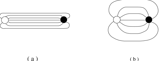
Figure 1.1: The colour field lines between quarks collapse upon themselves, due to the self interacting nature of the gluons, to form a flux-tube-like structure. At long distances (a) the fields lines collapse to become almost string-like and at short distances (b) the fields lines expand to become almost QED-like.

This particular model has been used in an attempt to model nuclear matter. Although it has an obvious shortcoming, in that it is more applicable to a pion gas, it does surprisingly well at predicting some of the overall bulk properties of nuclear matter [4, 5].

It is fairly straightforward to generalize this simple model to a more realistic one which involves triplets of quarks. Here the flux-tubes leaving each quark meets at a central vertex such that overall length, $r$, of “flux-tubing” is minimized (cf. figure 2.1.a). The potential energy is simply $\sigma r\,$ [6].

In a more general setting one could consider a full many-body quark potential in which large clusters of quarks may be connected by a single network of flux-tubes [4]; in general, this “gas” is assumed to consist of colourless objects. Again the potential energy is simply $\sigma r\,$, where $r$ is now the minimal amount of flux-tubing used for a given cluster of quarks. In such a model, there could exist very complex topological configurations of flux-tubes, such as long strands or web-like structures (figure 1.2).

Figure 1.2: Possible flux-tube configurations for an $SU_{\rm c}(3)$ quark gas in a box.

All of these models are completely motivated by results from lattice QCD, where variations are taken about minimal lattice field configurations between quarks.

1.1.1 Possible Phases of Nuclear Matter

There is a major advantage to understanding nuclear matter in terms of its constituent quarks. Not only is a deeper understanding of nuclear physics likely to be achieved, but also a more general understanding of the nature of quark matter. This understanding could possibly lead to the prediction of more exotic forms of matter. To illustrate this point let us now “hypothesize” some of the possible phases of nuclear/quark matter (figure 1.3) in the context of a general string-flip potential picture.

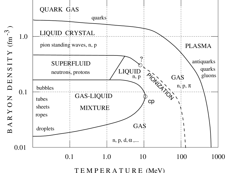
Figure 1.3: Postulated nuclear matter phase diagram (adapted from Siemens & Jensen [1].)

First consider nuclear matter in a box at low temperature (i.e., in its ground state) in a standard nuclear model, with no references to quarks. At very low density the system is a gas of isolated nucleons with a Fermi degeneracy pressure on the walls of the box. As the box is gradually squeezed some of the nucleons may come close enough to start clumping together. At this stage the pressure becomes negative due to the clumping forces which are trying to reduce the volume. As the box is squeezed even further, short-range repulsion and other saturation mechanisms [1, 7] cause the pressure to become positive. Effectively the system behaves very much like water vapor; little droplets of nucleons floating around in a box. Further squeezing of the box causes liquid (probably a superfluid) to be formed.

Now consider a very simple flux-tube model where the many-body potential contains only three-body forces between red ($r$), green ($g$), and blue ($b$) quarks: each nucleon is represented by three valence quarks, $rgb$, connected by a triangular web of flux-tubes (cf. figure 2.1.a). In a flux-tube picture it is suspected that the role of meson exchange between nucleons in the nuclear physics picture is mimicked by the swapping of flux-tubes as nucleons move close to each other [8]. At sufficiently low pressure the system behaves as a gas of nucleons because the clusters of quarks are essentially isolated from one another: no flux-tubes are exchanged. In addition, as the quarks are fermions a Fermi pressure is set up on the walls of the box but not within the $rgb$ clusters themselves. As the box is squeezed some of the clusters come into contact with each other causing a clumping effect. The saturation effect is perhaps not that obvious, however it has been shown that this simple flux-tube picture does indeed lead to saturation of nuclear forces [4, 5, 9]. It even produces the subtle effect of nucleon swelling in nuclear matter. However it does not appear to produce a strong enough attractive force to produce binding; speculation as to “why?” will be discussed later on in this thesis. “Further squeezing of the box causes a liquid (probably a superfluid) to be formed.” Presumably if spin correlations were set up between pairs of clusters of quarks, collective states that indicate superfluidity may be detected. This idea has not been tested. The possibility of new physics is introduced when the box is squeezed further. At such densities the nucleon could perhaps form a liquid crystal [10], as it might be more energetically favourable for the planes of the $rgb$ clusters to align themselves. If the box is squeezed even further the flux-tubes essentially dissolve leaving a Fermi gas of quarks.

If the temperature of the box is now increased, even more phases of nuclear matter become evident. For very low densities the system remains a Fermi gas of nucleons, but now it may become an excited Fermi gas. As the box is squeezed the nucleons may clump to form a gas-liquid mixture provided the temperature is not too high. If the temperature is too high it may simply stay in its gaseous phase. As the box is squeezed further each of the aforementioned possible states will go over into a liquid. If the temperature and pressure is just right it is possible for all three phases of nuclear matter to coexist: cf. figure 1.3.

If the temperature at low density is pushed higher the gas pionizes (figure 1.3): the mesons go on shell. In order for this to work in a flux-tube model a meson production mechanism would have to be incorporated. Perhaps the simplest incorporation would be to introduce a string breaking mechanism, figure 1.4, then if the flux-tubes became too long they would break, producing mesons. If the temperature is further increased a plasma of quarks, antiquarks, and gluons would be produced.

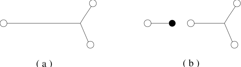
Figure 1.4: A naïve meson production scheme. If a flux-tube is stretched long enough such that there is enough mass energy in a segment to produce a $q\bar{q}$ pair of mass $2m_{q}$ then the string (flux-tube) will break creating a pair of quarks, with the corresponding segment vanishing, with probability $\sim e^{-\pi m_{q}^{2}/\sigma}$ [11]. Note that this model does not include a mechanism for getting rid of the mesons.

Finally, by varying the temperature and pressure of the aforementioned phases other phases can be reached: if the temperature is increased in the liquid crystal phase (see figure 1.3) the liquid crystal will eventually become disrupted forming, perhaps, a pionized gas or a plasma. If the pressure or temperature of the liquid phase is raised a liquid crystal, pionized gas, or plasma may be formed (this suggests perhaps another triple point on the phase diagram).

A summary of the various phases of nuclear matter that have been discussed is illustrated in figure 1.3. It should be emphasized that all of this is speculative and model dependent, i.e., the only experiments that exist are in the region $T\,\raisebox{-2.69096pt}{$\stackrel{{\scriptstyle<}}{{\sim}}$}\,{\cal O}({1})MeV$ and $\rho\,\raisebox{-2.69096pt}{$\stackrel{{\scriptstyle<}}{{\sim}}$}\,{\cal O}({0.2})fm^{-3}$ [8].

1.1.2 A Crude Model of Nuclear Matter

It should now be apparent that attempting to construct a model of nuclear matter in terms of quarks is not a very simple task. To reduce this burden some simplifying assumptions or restrictions will have to be made. One restriction is to only consider low temperature phenomena. Some simplifying assumptions would be to require that the model correctly predict some of the very basic bulk properties of nuclear matter:

• nucleon gas at low densities with no van der Waals forces

• nucleon binding at higher densities

• nucleon swelling and saturation of nuclear forces with increasing density

• quark gas at extremely high densities

There are many models that attempt to reproduce all of these properties but none that reproduces them completely.

In this thesis only one particular class of models, called string-flip potential models [9, 4, 5], will be considered, in chapters 2 and 3. These models appear to be promising because they reproduce most of the aforementioned properties with the exception of nucleon binding.

1.2 Superstring Inspired ${\rm E}_{6}$ Models

The $\mbox{${\rm SU}({3})_{{\rm c}}$}\otimes\mbox{${\rm SU}({2})_{{\rm L}}$}\otimes\mbox{${\rm U}({1})_{{\rm Y}}$}$ standard model (SM) is a very successful model. It has thus far withstood rigorous experimental testing. However, despite its success the SM has many problems:

• no unification of the forces

• gauge hierarchical and fine tuning problems

• three generations of quarks and leptons for no particular reason

• too many parameters to be extracted from experiment

Some of the earlier attempts at unification tried to unify the strong and electroweak forces by embedding the $\mbox{${\rm SU}({3})_{{\rm c}}$}\otimes\mbox{${\rm SU}({2})_{{\rm L}}$}\otimes\mbox{${\rm U}({1})_{{\rm Y}}$}$ structure into higher groups, such as SU(5) and SO(10). These “grand unified theories”, or GUT’s, were only partially successful. The simplest of the GUT’s was SU(5) which seemed promising at the time because it predicted the ratio of the ${\rm SU}({2})_{{\rm w}}$ and ${\rm U}({1})_{{\rm em}}$ couplings and the proton lifetime [12]. However, the ordinary SU(5) GUT is no longer a possibility because more refined experimental measurements are now in disagreement with its predictions for the couplings and the proton lifetime [13]. In addition, this simple model had too many parameters and no explanation for family replication. The next likely candidate group was SO(10), although the three (or more) copies of the generational structure still had to be inserted by hand.

Difficulties with the SM and GUT models concerning gauge hierarchy and fine tuning problems led to theoretical remedies such as technicolour and supersymmetry (SUSY). The most appealing of these theories is SUSY, which has generators that relate particles of different spin in the same supermultiplet. The locality of these generators leads to supergravity models. SUSY (and its extended versions) however, did not have enough room for all of the SM particles [12]. To solve this problem direct product structures were made with SUSY and Yang-Mills gauge groups. These structures are now commonly referred to as “SUSY” models. Of course the price paid for this was a large particle spectrum (at least twice that of the SM) and the problem of family replication still remained.

In the early 1970’s some interest was sparked in ${\rm E}_{6}$ as a GUT when it was discovered that all the then known generations of fermions could be placed in a single 27 dimensional representation. This (“topless”) model was quite popular because the newly discovered $\tau$ lepton and $b$ quark could also be fitted neatly into the 27; there was no need for a third generation. However this model was quickly disallowed as it was experimentally shown that the $\tau$ and $b$ belonged to a third generation, and the idea of ${\rm E}_{6}$ as a GUT died.

$${\bf 27}=\left\{\framebox{$\left(\begin{array}[]{c}u\\ d\end{array}\right)_{\rm L}\left(\begin{array}[]{c}\nu_{e}\\ e\end{array}\right)_{\rm L}u_{\rm L}^{c}d_{\rm L}^{c}e_{\rm L}^{c}$}\;\nu_{e_{\rm L}}^{c}d_{\rm L}^{\prime}d_{\rm L}^{\prime c}\left(\begin{array}[]{c}\nu_{e}^{\prime}\\ e^{\prime}\end{array}\right)_{\rm L}\left(\begin{array}[]{c}e^{\prime}\\ \nu_{e}^{\prime}\end{array}\right)_{\rm L}^{c}\nu_{e_{\rm L}}^{\prime\prime c}\right\}$$

$${\bf 27}=\left\{\framebox{$\left(\begin{array}[]{c}c\\ s\end{array}\right)_{\rm L}\left(\begin{array}[]{c}\nu_{\mu}\\ \mu\end{array}\right)_{\rm L}c_{\rm L}^{c}s_{\rm L}^{c}\mu_{\rm L}^{c}$}\;\nu_{\mu_{\rm L}}^{c}s_{\rm L}^{\prime}s_{\rm L}^{\prime c}\left(\begin{array}[]{c}\nu_{\mu}^{\prime}\\ \mu^{\prime}\end{array}\right)_{\rm L}\left(\begin{array}[]{c}\mu^{\prime}\\ \nu_{\mu}^{\prime}\end{array}\right)_{\rm L}^{c}\nu_{\mu_{\rm L}}^{\prime\prime c}\right\}$$

$${\bf 27}=\left\{\framebox{$\left(\begin{array}[]{c}t\\ b\end{array}\right)_{\rm L}\left(\begin{array}[]{c}\nu_{\tau}\\ \tau\end{array}\right)_{\rm L}t_{\rm L}^{c}b_{\rm L}^{c}\tau_{\rm L}^{c}$}\;\nu_{\tau_{\rm L}}^{c}b_{\rm L}^{\prime}b_{\rm L}^{\prime c}\left(\begin{array}[]{c}\nu_{\tau}^{\prime}\\ \tau^{\prime}\end{array}\right)_{\rm L}\left(\begin{array}[]{c}\tau^{\prime}\\ \nu_{\tau}^{\prime}\end{array}\right)_{\rm L}^{c}\nu_{\tau_{\rm L}}^{\prime\prime c}\right\}$$

Figure 1.5: ${\rm E}_{6}$ particle content.^a The SM particles are shown in the boxes on the left and their “exotic” counterparts outside the boxes on the right. Although the exotics are labeled in a way that suggests they have the same quantum numbers as the non-exotics, in general they need not. The labeling for these particles in the literature has not been settled upon and varies quite significantly from paper to paper [13]. Here the labeling scheme was chosen to reflect a specific ${\rm E}_{6}$ model that will be constructed in this thesis. In particular, all the exotics will carry the “expected” quantum numbers as their non-exotic counter parts do, with the exception being L=0 (i.e., Lepton number zero) for the primed and double primed ones.

$\mbox{}^{a}$Note: Embedded in the 27’s is the symmetry group ${\rm SU}({2})_{{\rm I}}$ due to an ambiguity in the particle assignments $\left\{\left(\begin{array}[]{@{}c@{}}\nu_{l}\\ l\end{array}\right)_{\rm L}d_{\rm L}^{c}\right\}\;\Longleftrightarrow\;\left\{\left(\begin{array}[]{@{}c@{}}\nu_{l}^{\prime}\\ l^{\prime}\end{array}\right)_{\rm L}d_{\rm L}^{\prime c}\right\}$ and $\{\nu_{l_{\rm L}}^{c}\}\;\mbox{\tiny$\Longleftrightarrow$}\;\{\nu_{l_{\rm L}}^{\prime\prime c}\}\,$ (cf. figure 1.6.d). This ambiguity can easily be seen via the decomposition 27=$\sum_{\oplus}$(SO(10),SU(5)).

In late 1984 Green and Schwarz showed that 10 dimensional string theory is anomaly free if its gauge group is either ${\rm E}_{8}\otimes{\rm E}_{8}^{\prime}\;$or SO(32). The group that had received the most attention was ${\rm E}_{8}\otimes{\rm E}_{8}^{\prime}\;$as it led to chiral fermions, similar to those in the SM, whereas SO(32) did not. Furthermore, it was shown that compactification down to 4 dimensions (assuming N=1 SUSY) can lead to ${\rm E}_{6}$ as an “effective” GUT group. Each family of SM particles now sits in its own 27, figure 1.5. The generational problem may be solved because it is expected that any reasonable compactification scheme should generate the appropriate number of copies of the 27. For instance in a Calabi-Yau compactification scheme [14],

$$\mbox{${\rm E}_{8}\otimes{\rm E}_{8}^{\prime}\;$}\;\longrightarrow\;{\rm SU(3)}\otimes{\rm E}_{6}\otimes{\rm E}_{8}^{\prime}\;,$$

the number of generations is related to the topology of the compactified space. A further assertion that the matter fields remain supersymmetrically degenerate ensures proper management of any gauge hierarchical and fine tuning problems. It is assumed that the hidden sector, ${\rm E}_{8}^{\prime}$, which couples to the matter fields of ${\rm E}_{6}$ by gravitational interactions will provide a mechanism for lifting the degeneracy.

So the inspiration for using ${\rm E}_{6}$ is that if it proves to be a possible GUT then it opens up the possibility of finding a TOE (Theory Of Everything). However, it should be pointed out that ${\rm E}_{6}$ is not the only possible stop $en$ $route$ to the SM, but it is the most studied [13]. It is for this reason that the low energy phenomenology resulting from ${\rm E}_{6}$ will be studied in this thesis.

1.2.1 ${\rm E}_{6}$ Phenomenology

An extra ${\rm Z}_{\rm E}\,$

In order to produce SM phenomenology ${\rm E}_{6}$ must be broken. Also to handle any hierarchical and fine tuning problems, SUSY must be preserved [14]. This restriction makes the task more difficult, using most naïve breaking schemes. The solution to the problem was found by using a Wilson-loop mechanism [14] over the non-simply-connected-compactified-string-manifold to factor out the various subgroups of ${\rm E}_{6}$ . Figure 1.6 shows some of the possible, popular, rank 5 and rank 6 groups that can be produced by this scheme.

(a)	${\rm E}_{6}$	$\longrightarrow$	$\mbox{${\rm SU}({3})_{{\rm c}}$}\otimes\mbox{${\rm SU}({2})_{{\rm L}}$}\otimes\mbox{${\rm U}({1})_{{\rm Y}}$}$ $\otimes$${\rm U}({1})_{{\rm Y_{E}}}$
(b)	${\rm E}_{6}$	$\longrightarrow$	$\left.\mbox{\begin{tabular}[]{@{}l}SO(10)$\otimes$U(1)${}_{\psi}$\\ \mbox{ \begin{picture}(6.0,7.0)\put(0.0,7.0){\line(0,-1){6.0}} \put(0.0,1.0){\vector(1,0){6.0}} \end{picture} } SU(5)$\otimes$U(1)${}_{\chi}$\end{tabular}}\right\}$ $\stackrel{{\scriptstyle\mbox{\scriptsize ER5M}}}{{\longrightarrow}}$ $\mbox{${\rm SU}({3})_{{\rm c}}$}\otimes\mbox{${\rm SU}({2})_{{\rm L}}$}\otimes\mbox{${\rm U}({1})_{{\rm Y}}$}$ $\otimes$U(1)θ ($i.e.$, U(1)${}_{\psi}\otimes$U(1)${}_{\chi}\rightarrow$U(1)θ in the large VEV limit.)
(c)	${\rm E}_{6}$	$\longrightarrow$	$\mbox{${\rm SU}({3})_{{\rm c}}$}\otimes\mbox{${\rm SU}({2})_{{\rm L}}$}\otimes\mbox{${\rm SU}({2})_{{\rm R}}$}\otimes\mbox{}\underbrace{\mbox{${\rm U}({1})_{{\rm L}}$}\otimes\mbox{${\rm U}({1})_{{\rm R}}$}}_{\mbox{\hskip 45.5244pt}\raisebox{8.53581pt}{\rm\scriptsize ER5M}\mbox{ \begin{picture}(6.0,7.0)\put(0.0,7.0){\line(0,-1){6.0}} \put(0.0,1.0){\vector(1,0){6.0}} \end{picture} }\mbox{${\rm U}({1})_{{\rm V=L+R}}$}}$
(d)	${\rm E}_{6}$	$\longrightarrow$	$\mbox{${\rm SU}({3})_{{\rm c}}$}\otimes\mbox{${\rm SU}({2})_{{\rm L}}$}\otimes\mbox{${\rm U}({1})_{{\rm Y}}$}\otimes\mbox{}\underbrace{\mbox{${\rm SU}({2})_{{\rm I}}$}\otimes{\rm U}(1)^{\prime}}_{\mbox{\hskip 22.76219pt}\raisebox{8.53581pt}{\rm\scriptsize ER5M}\mbox{ \begin{picture}(6.0,7.0)\put(0.0,7.0){\line(0,-1){6.0}} \put(0.0,1.0){\vector(1,0){6.0}} \end{picture} }\mbox{${\rm SU}({2})_{{\rm I}}$}}$

Figure 1.6: ${\rm E}_{6}$ Wilson-loop-breaking schemes [13]. (a) shows a rank-5 model and (b) through (d) show rank-6 models. Scheme (a) gives the SM plus an extra ${\rm U}({1})_{{\rm Y_{E}}}$. Schemes (b) through (d) can produce effective rank-5 models, ER5M, by taking a large VEV limit.

As it can be seen, the various breaking schemes always give rise to extra vector bosons beyond the SM: in fact it is unavoidable. In this thesis only the simplest of these models (figure 1.6.a) which generates an extra vector boson, the ${\rm Z}_{\rm E}\,$, will be considered.

The Supermatter Fields

The most general superpotential that is invariant under $\mbox{${\rm SU}({3})_{{\rm c}}$}\otimes\mbox{${\rm SU}({2})_{{\rm L}}$}\otimes\mbox{${\rm U}({1})_{{\rm Y}}$}$ and renormalizable for the fields given in figure 1.5 is of the form (neglecting various isospin contractions and generational indices) [13],

$$W=W_{0}+W_{1}+W_{2}+W_{3}$$ (1.2)

$$\begin{array}[]{@{}l@{}l@{}l@{}}W_{0}&=&\lambda_{1}\mbox{$\Phi_{{{{\rm R}^{\prime}}}}$}\mbox{$\Phi_{{Q}}$}\mbox{$\Phi_{{u_{\rm L}^{c}}}$}+\lambda_{2}\mbox{$\Phi_{{{{\rm L}^{\prime}}}}$}\mbox{$\Phi_{{Q}}$}\mbox{$\Phi_{{d_{\rm L}^{c}}}$}+\lambda_{3}\mbox{$\Phi_{{{{\rm L}^{\prime}}}}$}\mbox{$\Phi_{{L}}$}\mbox{$\Phi_{{e_{\rm L}^{c}}}$}+\lambda_{4}\mbox{$\Phi_{{{{\rm R}^{\prime}}}}$}\mbox{$\Phi_{{{{\rm L}^{\prime}}}}$}\mbox{$\Phi_{{\nu_{e_{\rm L}}^{\prime\prime c}}}$}+\lambda_{5}\mbox{$\Phi_{{d_{\rm L}^{\prime}}}$}\mbox{$\Phi_{{d_{\rm L}^{\prime c}}}$}\mbox{$\Phi_{{\nu_{e_{\rm L}}^{\prime\prime c}}}$}\\ W_{1}&=&\lambda_{6}\mbox{$\Phi_{{d_{\rm L}^{\prime}}}$}\mbox{$\Phi_{{u_{\rm L}^{c}}}$}\mbox{$\Phi_{{e_{\rm L}^{c}}}$}+\lambda_{7}\mbox{$\Phi_{{L}}$}\mbox{$\Phi_{{d_{\rm L}^{\prime c}}}$}\mbox{$\Phi_{{Q}}$}+\lambda_{8}\mbox{$\Phi_{{\nu_{e_{\rm L}}^{c}}}$}\mbox{$\Phi_{{d_{\rm L}^{\prime}}}$}\mbox{$\Phi_{{d_{\rm L}^{c}}}$}\\ W_{2}&=&\lambda_{9}\mbox{$\Phi_{{d_{\rm L}^{\prime}}}$}\mbox{$\Phi_{{Q}}$}\mbox{$\Phi_{{Q}}$}+\lambda_{10}\mbox{$\Phi_{{d_{\rm L}^{\prime c}}}$}\mbox{$\Phi_{{u_{\rm L}^{c}}}$}\mbox{$\Phi_{{d_{\rm L}^{c}}}$}\\ W_{3}&=&\lambda_{11}\mbox{$\Phi_{{{{\rm R}^{\prime}}}}$}\mbox{$\Phi_{{L}}$}\mbox{$\Phi_{{\nu_{e_{\rm L}}^{\prime\prime c}}}$}\,.\end{array}$$

$\mbox{$\Phi_{{A}}$}=\Phi(A,\tilde{A})$ is the superfield, such that $A={{\rm R}^{\prime}},Q,u_{\rm L}^{c},$… , and

$$\begin{array}[]{cccc}\mbox{$\Phi_{{Q}}$}=\left(\begin{array}[]{@{}c@{}}{\mbox{$\Phi_{{u}}$}}\\ {\mbox{$\Phi_{{d}}$}}\end{array}\right)_{\rm L}\,,&\mbox{$\Phi_{{L}}$}=\left(\begin{array}[]{@{}c@{}}{\mbox{$\Phi_{{\nu_{e}}}$}}\\ {\mbox{$\Phi_{{e}}$}}\end{array}\right)_{\rm L}\,,&\mbox{$\Phi_{{{{\rm L}^{\prime}}}}$}=\left(\begin{array}[]{@{}c@{}}{\mbox{$\Phi_{{\nu_{e}^{\prime}}}$}}\\ {\mbox{$\Phi_{{e^{\prime}}}$}}\end{array}\right)_{\rm L}\,,&\mbox{$\Phi_{{{{\rm R}^{\prime}}}}$}=\left(\begin{array}[]{@{}c@{}}{\mbox{$\Phi_{{e^{\prime}}}$}}\\ {\mbox{$\Phi_{{\nu_{e}^{\prime}}}$}}\end{array}\right)_{\rm L}^{c}\,,\end{array}$$

for the first generation of the 27’s, and similarly for the other generations. The Yukawa couplings, $\lambda_{i}$’s, also carry generational indices which have been suppressed; the couplings are inter-generational as well as intra-generational. The superpotential, W, summarizes the entire possible spectrum of low energy physics which can occur within the context of an ${\rm E}_{6}$ framework.

Notice that $W$ was only required to be invariant under the SM gauge group. Further constraints from ${\rm E}_{6}$ model building may cause some of the $\lambda_{i}$ terms to disappear. Furthermore, not all of these terms can simultaneously exist without giving rise to $\Delta$L$\neq 0$ and $\Delta$B$\neq 0$ interactions; ${\rm E}_{6}$ models say nothing about the assignments of baryon (B) and lepton (L) number until they are connected to SM representations. As a result various scenarios may occur,

$\bullet$   Leptoquarks :	B($q^{\prime}_{\rm L}$)=	$\frac{1}{3}\,$, L($q^{\prime}_{\rm L}$)=1  $\Longrightarrow$	$\lambda_{{9}}$=$\lambda_{{10}}$=0
$\bullet$   Diquarks :	B($q^{\prime}_{\rm L}$)=	$-\,\frac{2}{3}\,$, L($q^{\prime}_{\rm L}$)=0  $\Longrightarrow$	$\lambda_{{6}}$=$\lambda_{{7}}$=$\lambda_{{8}}$=0
$\bullet$   Quarks :	B($q^{\prime}_{\rm L}$)=	$\frac{1}{3}\,$, L($q^{\prime}_{\rm L}$)=0  $\Longrightarrow$	$\lambda_{{6}}$=$\lambda_{{7}}$=$\lambda_{{8}}$=$\lambda_{{9}}$=$\lambda_{{10}}$=0

where it has been assumed that L($\nu_{l_{\rm L}}^{c}$)= $-1\,$ (these scenarios assume that there exist only three copies of the 27; more complicated ones can be constructed by adding extra copies). In this thesis the least exotic of these models, i.e., the “Quarks,” will be investigated. Furthermore, to avoid any fine tuning problems with the neutrino masses,

$$m_{\nu_{e_{\rm L}}^{c}}\;<<\;m_{e}\;\Longleftrightarrow\;\mbox{$\lambda_{{11}}$}<<\mbox{$\lambda_{{3}}$}\,,$$

it will be assumed $\lambda_{{11}}$=0.

In this model the masses of the particles are generated by letting the role of the Higgs fields be played by

$$\begin{array}[]{ccc}{\tilde{\rm L}^{\prime}}=\left(\begin{array}[]{@{}c@{}}{\tilde{\nu}^{\prime}_{e_{\rm L}}}\\ {\tilde{e}^{\prime}_{\rm L}}\end{array}\right)\,,&{\tilde{\rm R}^{\prime}}=\left(\begin{array}[]{@{}c@{}}{\tilde{e}^{\prime c}_{\rm L}}\\ {\tilde{\nu}^{\prime c}_{e_{\rm L}}}\end{array}\right)\,,&\tilde{\nu}^{\prime\prime c}_{e_{\rm L}}\,,\end{array}$$

for each generation. It is possible to work in a basis where only the third generation of Higgses acquire a VEV; the remainder become “unHiggses” [13, 15]. In this basis the Yukawa couplings,

$$\lambda_{4}^{ijk}\mbox{$\Phi_{{{{\rm R}^{\prime}}_{i}}}$}\mbox{$\Phi_{{{{\rm L}^{\prime}}_{j}}}$}\mbox{$\Phi_{{\nu^{\prime\prime}_{l_{k}}}}$}\,,$$

where $i,j,k=1,2,3$ are generational indices, takes on a much simpler form,

$$\lambda_{4}\;\in\;\{\lambda_{4}^{ijk}|\lambda_{4}^{i33}=\lambda_{4}^{3i3}=\lambda_{4}^{33i}=0\,,\;\lambda_{4}^{333}=\lambda_{4}^{3jk}=\lambda_{4}^{j3k}=\lambda_{4}^{jk3}\neq 0\;{\rm s.t.}\;i=1,2\;\&\;j,k=1,2,3\}\,.$$

This basis also eliminates the potential problem of flavour changing neutral currents at the tree level. It is also assumed that the $\lambda_{i}$’s are real and that the couplings to the unHiggses are very small. The former assumption helps to further simplify the model and reduce any effects it might have in the CP violating sector [13].

1.2.2 Heavy Lepton Production

${\rm E}_{6}$ models are very rich in their spectrum of possible low energy phenomenological predictions. If any new particles are found that fit within this framework then perhaps it will lead the way to a more unified theory of the fundamental forces of nature. However this is no small task, for a full theory would have to be able to actually predict the mass spectrum of the particles and the relationships between various couplings, and yet require very few parameters. Superstring inspired ${\rm E}_{6}$ models are far from being able to complete this task. However, proof that ${\rm E}_{6}$ is an effective GUT would be a good first step. But even this would not necessarily qualify superstrings to be the next step for it is not totally inconceivable that some other theory might give rise to ${\rm E}_{6}$ as an effective GUT — $caveat$ $emptor$.

A natural question to ask would be, “Where to look for ${\rm E}_{6}$ phenomenology?” High energy hadron colliders, such as the Tevatron at Fermilab (1.8 TeV c.o.m., ${\cal L}\sim 10^{2}pb^{-1}/yr\,$, $p\bar{p}$) or the LHC (14 TeV c.o.m., ${\cal L}\sim 10^{5}pb^{-1}/yr\,$, $pp$), offer possibilities of observing phenomena beyond the SM by looking for the production of heavy leptons through a mechanism known as gluon-gluon fusion, see figure 1.7.

Figure 1.7: Gluon-gluon fusion to two heavy leptons, $gg$ $\longrightarrow$ L⁺L^-. The loop contains quarks, $q\,$, which couple to vector bosons, $Z_{i=1,2}$, scalar-Higgses, $H^{0}_{i=1,2,3}$, and a pseudo-scalar-Higgs, $P^{0}\,$, and squarks, $\tilde{q}\,$, which couple to scalar-Higgses.

This is an interesting process because there are enhancements in the cross-sections related to the heavy (s)fermions running around in the loop. The computation was done in the minimal supersymmetric standard model (MSSM) by Cieza Montalvo, $et$ $al.$, [16] in which they predict ${\cal O}(10^{5})\,events/yr$. Therefore for ${\rm E}_{6}$ it is expected that the production rate should in principle be higher since there are more particles running around in the loop. This process will be investigated in this thesis.

1.3 Summary

String-flip potential models and superstring-inspired-${\rm E}_{6}$ models have been discussed in a general setting. In this thesis various aspects of these models will be discussed. In chapter 2 the ${\rm SU}({3})_{{\rm c}}$ string-flip-potential model will be investigated and put into perspective with more generalized models. In chapter 3 modifications to the general string-flip-potential will be investigated. In chapter 4 heavy lepton production via gluon-gluon fusion will be investigated in an ${\rm E}_{6}$ framework. Chapter 5 will contain an overall summary of the work done in this thesis.

Chapter 2 The SU(3) String-Flip Potential Model

2.1 Introduction

In this chapter a string-flip potential model for 3-quark systems will be constructed. Some simplifying assumptions about flux-tube minimization will be made in order to reduce the Monte Carlo computation time. The results for a linear potential model, $\mathrm{SU}_{\ell}(3)$, and a harmonic oscillator potential model, $\mathrm{SU}_{h}(3)$, in which the colour has been fixed to a given quark, will be presented. The results will be compared with an $\mathrm{SU}_{h}(3)$ model proposed by Horowitz and Piekarewicz [4] in which different simplifying assumptions, about the minimal flux-tube topology, were made. Also a comparison of their results [4] with some earlier work done by Watson [5] on $\mathrm{SU}(2)$ will be made. The chapter concludes with a discussion on possible future directions to pursue in order to obtain bound state nuclear matter.

2.2 The General String-Flip Potential Model

As mentioned in the previous chapter a crude quark model of nuclear matter would be expected to have to at least the following properties: at low densities the quarks should condense out to form isolated baryons; at a higher density, the interaction between quarks should lead to positive binding energy between nucleons and a swelling of nucleons; and at still higher densities, it is expected that the hadrons should dissolve into a quark-gluon plasma. This last assumption is in contrast to the traditional nucleon models, which require the forces to be carefully adjusted so that they saturate at infinite density, effectively implying a hard core. Some simple models which appear to be likely candidates are string-flip potential models [4, 5], and to some extent linked cluster expansion models [17].

The cluster models are based on one-gluon exchange potentials and use an N-body harmonic oscillator potential, i.e.,

$$V_{\mathrm{conf}}=\frac{1}{2}k\sum_{i<j}({\vec{\mathrm{r}}}_{i}-{\vec{\mathrm{r}}}_{j})^{2}\,,$$ (2.1)

to mimic quark confinement. These models are mainly used for describing short range nuclear effects, as they suffer from van der Waals forces due to the nature of the confining potential. Despite this shortcoming, they appear to be quite useful in explaining local effects such as nucleon swelling (fat nucleons) [18], quark clustering preferences, and relative strengths of the various one-gluon exchange potentials [17].

The string-flip potential models are, on the other hand, motivated by lattice QCD. These models postulate how flux-tubes should form amongst the quarks at zero temperature based on some input from lattice QCD. An adiabatic assumption is made, in which the quarks move slowly enough for their fields to reconfigure themselves, such that the overall potential energy is minimized: i.e.,

$$V=\min\{\sum_{\{q_{m}\ldots q_{n}\}}\mathrm{v}({\vec{\mathrm{r}}}_{m}\ldots{\vec{\mathrm{r}}}_{n})\,|\,\bigcup_{\{m\ldots n\}}^{\sim}\{q_{m}\ldots q_{n}\}=\{q_{1}\ldots q_{N_{q}}\}\}\;,$$ (2.2)

where the $N_{q}$ quarks are placed in a cube of side $L$ and subjected to periodic boundary conditions to simulate continuous quark matter. The sum is over all gauge invariant sets $\{q_{m}\ldots q_{n}\}$ of quarks, such that at least one element from each set lies inside a common box, whose disjoint union, $\stackrel{{\scriptstyle\mbox{\footnotesize$\sim$}}}{{\cup}}\,$, makes up the complete colour singlet set $\{q_{1}\ldots q_{N_{q}}\}$ of $N_{q}$ quarks. It is easy to see that this potential allows for complete minimal quark clustering separability at low densities without suffering from van der Waals forces. At present, these models [4, 5] are quite crude in that they do not include short range one gluon exchange phenomena and spin effects and are flavour degenerate. Despite their shortcomings, in general, these models seem quite capable of correctly describing most of the bulk nuclear properties, with the exception of nuclear binding.

It is known that the $\mathrm{SU}(2)$ string-flip potential models do show these properties, except for the positive binding energy which probably arises from short range forces. However, the only existing extension to an $\mathrm{SU}(3)$ model [4] leads to the rather surprising result that the nucleon appears to shrink in nuclear matter. It is therefore of some interest to repeat the calculation of [4], in an attempt to determine whether the approximations made there alter qualitatively the solution.

2.3 $\mathrm{SU}(3)$ String-Flip Model

The string-flip model involves solving a Hamiltonian system of fermions governed by the potential given in equation (2.2). To solve this system requires the use of variational Monte Carlo techniques [19]. In order to compute any observable in a finite amount of time further assumptions about the form of the potential must be made.

In this model the potential is restricted

• to summing over sets of colour singlet clusters of three quarks,

  $$V=\min\{\sum_{\{q_{r}q_{g}q_{b}\}}\mathrm{v}({\vec{\mathrm{r}}}_{\mathrm{r}},{\vec{\mathrm{r}}}_{\mathrm{g}},{\vec{\mathrm{r}}}_{\mathrm{b}})|\,\bigcup_{\{rgb\}}^{\sim}\{q_{r}q_{g}q_{b}\}=\{q_{1}\ldots q_{N_{q}}\}\}\;,$$ (2.3)

• such that the colour of a given quark is fixed.

Assumption $a$ does have some validity as it has been shown, via a linked quark cluster model, that it is energetically more favourable for $6q$ systems to dissociate into two nucleons as a result of hyperfine interactions [17, 20, 21]. However, this is not necessarily the case at lower densities, as the linked cluster models are unreliable here. Assumption $b$, that of fixed colour, greatly restricts the number of possible field configurations and therefore reduces the chance of finding an absolute minimum. At low densities this should not have any effect on the potential, as the system consists of isolated nucleons. Similarly at high densities no effect is expected, as the system consists of uncorrelated quarks. At intermediate densities some effects might be expected, particularly around any regions in which a phase transition might occur.

For the $\mathrm{SU}_{\ell}(3)$ model, the potential, V, has the components [6]

$${\mathrm{v}}_{\ell}({\vec{\mathrm{r}}}_{\mathrm{r}},{\vec{\mathrm{r}}}_{\mathrm{g}},{\vec{\mathrm{r}}}_{\mathrm{b}})=\sigma\left\{\begin{array}[]{lr}{\mathrm{r}}_{\mathrm{br}}+{\mathrm{r}}_{\mathrm{rg}}&\mathrm{if}\;\angle\,brg\,\geq\,120^{\circ}\\ {\mathrm{r}}_{\mathrm{rg}}+{\mathrm{r}}_{\mathrm{gb}}&\mathrm{if}\;\angle\,rgb\,\geq\,120^{\circ}\\ {\mathrm{r}}_{\mathrm{gb}}+{\mathrm{r}}_{\mathrm{br}}&\mathrm{if}\;\angle\,gbr\,\geq\,120^{\circ}\\ \\ \frac{1}{\sqrt{2}}\sqrt{3\xi^{2}+\sqrt{3}A}&\mathrm{otherwise}\end{array}\right.\;,$$ (2.4)

where ${\vec{\mathrm{r}}}_{ij}={\vec{\mathrm{r}}}_{i}-{\vec{\mathrm{r}}}_{j}\,$, $\xi$ or

$$\xi_{\mathrm{rgb}}=\frac{1}{\sqrt{3}}\sqrt{{\mathrm{r}}_{\mathrm{rg}}^{2}+{\mathrm{r}}_{\mathrm{gb}}^{2}+{\mathrm{r}}_{\mathrm{br}}^{2}}\,,$$ (2.5)

and

$$A=\frac{1}{4}\sqrt{({\mathrm{r}}_{\mathrm{rg}}+{\mathrm{r}}_{\mathrm{gb}}+{\mathrm{r}}_{\mathrm{br}})(-{\mathrm{r}}_{\mathrm{rg}}+{\mathrm{r}}_{\mathrm{gb}}+{\mathrm{r}}_{\mathrm{br}})({\mathrm{r}}_{\mathrm{rg}}-{\mathrm{r}}_{\mathrm{gb}}+{\mathrm{r}}_{\mathrm{br}})({\mathrm{r}}_{\mathrm{rg}}+{\mathrm{r}}_{\mathrm{gb}}-{\mathrm{r}}_{\mathrm{br}})}$$ (2.6)

is the area inclosed by the triangle $\triangle rgb\,$ (see figure 2.1.a). For $\mathrm{SU}_{h}(3)$ the components are

$${\mathrm{v}}_{h}({\vec{\mathrm{r}}}_{\mathrm{r}},{\vec{\mathrm{r}}}_{\mathrm{g}},{\vec{\mathrm{r}}}_{\mathrm{b}})=\frac{1}{2}k\xi_{\mathrm{rgb}}^{2}\;$$ (2.7)

(see figure 2.1.b). This potential was obtained by replacing the linear segments of ${\mathrm{v}}_{\ell}$ by springs when the quarks, which were assumed to be of equal mass, formed a triangle with interior angles less than $120^{\circ}\,$ (cf. figure 2.5.a). This analogue model is expected to have similar features to $\mathrm{SU}_{\ell}(3)$ for $s$-wave $(qqq)$ states.

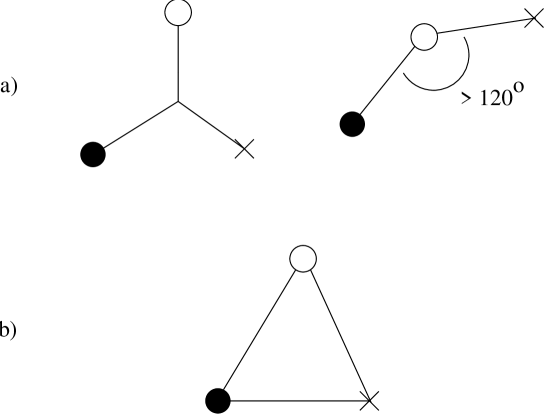
Figure 2.1: Flux-tube arrangements for the 3q cluster potentials a) ${\mathrm{v}}_{\ell}$ and b) ${\mathrm{v}}_{h}$.

The sum in equation (2.3) can be re-ordered by restricting it to run over all sets, $\{\mathrm{rgb}\}_{L}$, of quark triplets contained in a central box, such that the potential $\mathrm{v}({\vec{\mathrm{r}}}_{\mathrm{r}},{\vec{\mathrm{r}}}_{\mathrm{g}},{\vec{\mathrm{r}}}_{\mathrm{b}})$ is minimized with respect to all possible periodic permutations of the vectors $\{{\vec{\mathrm{r}}}_{\mathrm{r}},{\vec{\mathrm{r}}}_{\mathrm{g}},{\vec{\mathrm{r}}}_{\mathrm{b}}\}$, with the constraint that at least one of the vectors lies inside the central box: i.e.,

$$V=\min\{\sum_{\{\mathrm{rgb}\}_{L}}v({\vec{\mathrm{r}}}_{\mathrm{r}},{\vec{\mathrm{r}}}_{\mathrm{g}},{\vec{\mathrm{r}}}_{\mathrm{b}})\}\,,$$ (2.8)

where

$$v({\vec{\mathrm{r}}}_{\mathrm{r}},{\vec{\mathrm{r}}}_{\mathrm{g}},{\vec{\mathrm{r}}}_{\mathrm{b}}) = \min\{\mathrm{v}({\vec{\mathrm{r}}}_{\mathrm{r}}+L\vec{k}_{r},{\vec{\mathrm{r}}}_{\mathrm{g}}+L\vec{k}_{g},{\vec{\mathrm{r}}}_{\mathrm{b}}+L\vec{k}_{b})|\;(\vec{k}_{q})_{a}=-1,0,1$$ (2.9)

$$\;\;\;\;\;\;\mbox{ \& at least one }\vec{k}_{q}=\vec{0}\}\,.$$

This means that for quark triplets a search of one box deep from the central box is required, giving a total of $27^{2}$ possible permutations, in order to minimize a given $\mathrm{v}({\vec{\mathrm{r}}}_{\mathrm{r}},{\vec{\mathrm{r}}}_{\mathrm{g}},{\vec{\mathrm{r}}}_{\mathrm{b}})$ (see figure 2.2). These permutations can be reduced to $3$ by requiring that at least two sides of the triangle $\triangle rgb\,$, formed by a given permutation of quarks, be a minimum: i.e.,

$$v({\vec{\mathrm{r}}}_{\mathrm{r}},{\vec{\mathrm{r}}}_{\mathrm{g}},{\vec{\mathrm{r}}}_{\mathrm{b}})=\min\{\mathrm{v}(\delta{\vec{\mathrm{r}}}_{\mathrm{rg}},\delta{\vec{\mathrm{r}}}_{\mathrm{gb}},{\vec{\mathrm{r}}}_{\mathrm{br}}),\mathrm{v}({\vec{\mathrm{r}}}_{\mathrm{rg}},\delta{\vec{\mathrm{r}}}_{\mathrm{gb}},\delta{\vec{\mathrm{r}}}_{\mathrm{br}}),\mathrm{v}(\delta{\vec{\mathrm{r}}}_{\mathrm{rg}},{\vec{\mathrm{r}}}_{\mathrm{gb}},\delta{\vec{\mathrm{r}}}_{\mathrm{br}})\}\,,$$ (2.10)

where $\delta{\vec{\mathrm{r}}}_{\mathrm{ij}}$ is the minimum distance vector between the points ${\vec{\mathrm{r}}}_{i}$ and ${\vec{\mathrm{r}}}_{j}$, in a box of side $L$ with periodic boundary conditions, which is given by

$$(\delta{\vec{\mathrm{r}}}_{\mathrm{ij}})_{a}=\left\{\begin{array}[]{ll}({\vec{\mathrm{r}}}_{i}-{\vec{\mathrm{r}}}_{j})_{a}+L&\mathrm{if}\;\;({\vec{\mathrm{r}}}_{i}-{\vec{\mathrm{r}}}_{j})_{a}\;\,<\,-L/2\\ ({\vec{\mathrm{r}}}_{i}-{\vec{\mathrm{r}}}_{j})_{a}&\mathrm{if}\;|({\vec{\mathrm{r}}}_{i}-{\vec{\mathrm{r}}}_{j})_{a}|\,<\,\;\;L/2\\ ({\vec{\mathrm{r}}}_{i}-{\vec{\mathrm{r}}}_{j})_{a}-L&\mathrm{if}\;\;({\vec{\mathrm{r}}}_{i}-{\vec{\mathrm{r}}}_{j})_{a}\;\,>\,\;\;L/2\end{array}\right.\,,$$ (2.11)

where $a=x,y,z\,$. This is exact for $\mathrm{SU}_{h}(3)$; for $\mathrm{SU}_{\ell}(3)$, classical Monte Carlo shows that about $19\%$ of the events deviate from the exact answer by $\sim\,0.3\%$, on average.

Figure 2.2: A 2-D slice showing a typical flux-tube arrangement for three quarks, placed inside a central cube, subjected to periodic boundary conditions.

The number of different elements in the set, $\{\mbox{\footnotesize$\sum$}v\}$, from which the minimum must be extracted in order to obtain V, defined by equation (2.8), is $(N_{n}!)^{2}$ (where $N_{n}=N_{q}/3$ is the number of nucleons in the central box). For example, if $N_{n}=7$ this would yield $25\,401\,600$ elements! These elements can be reduced by fragmenting the set $\{q_{1}\ldots q_{N_{q}}\}$ into smaller pieces, or subclusters, such that each element can find $N_{br}$ complementary coloured pairs of quarks that are “closest” to it. These subclusters can be further fragmented, by “softening” the requirement that at least $N_{br}$ complementary pairs exist: i.e., by searching for disjoint subclusters. These subclusters are referred to as softened subclusters. The “closeness” of quark $q_{r}$ to the complementary pair $(q_{g}q_{b})$ is defined by the function $\delta_{r,(gb)}=v({\vec{\mathrm{r}}}_{\mathrm{r}},{\vec{\mathrm{r}}}_{\mathrm{g}},{\vec{\mathrm{r}}}_{\mathrm{b}})$, given in equation (2.9). The fragmented sets are thus constructed by computing an $N_{n}\times N_{n}^{2}$ matrix ($\Delta$) with elements $\delta_{r,(gb)}$, and then converting it into block diagonal form ($\Delta^{d}$) increasing in size from top to bottom, by swapping rows and columns such that each block diagonal element contains the elements of a fragmented set and all the off block diagonal elements are set to zero. The elements of $\{\mbox{\footnotesize$\sum$}v\}$ are now constructed by extracting permutations of elements $\delta_{r,(gb)}$, from unique columns and rows, of the block diagonal elements of $\Delta^{d}\,$. Further computational speed is gained by discarding sums that start to exceed the current minimum. In general, the fragmented sets constructed from $\{q_{1}\ldots q_{N_{0}}\}$, are not all disjoint from one another, and therefore the block diagonal elements of $\Delta^{d}$ may overlap. The degree of overlap increases with increasing density, causing the Monte Carlo to slow down.

This fragmentation procedure, or nearest neighbour search of depth $N_{br}$ (cf. [5]), reduces computation time quite significantly. The cost is that rare configurations with flux-tubes that stretch across the box or across unsoftened subclusters, that give a global minimum, might be missed. Preliminary Monte Carlo results show that the inclusion of softened subclusters yields no noticeable change. However, for a full $(N_{n}!)^{2}$ brute force search, performing a Monte Carlo becomes virtually impossible. A few brute force computations of the potential were made, for particles randomly thrown into a box, which seem to suggest that the fragmentation procedure is good to about $1\%\,$, with $N_{br}\approx 4$. $\mathrm{SU}_{\ell}(2)$ models also give similar results [5].

The validity of the fragmentation procedure can also be argued on physical grounds, for it is reasonable to assume that long flux-tube configurations would tend to dissociate into $q\bar{q}$ pairs. Therefore, the fragmentation procedure can be considered as a valid low temperature approximation.

The choice of variational wave function should attempt to reflect the overall bulk properties of the system. Here the wave function was chosen to be of the form,

$$\Psi(\alpha,\beta,\rho)=\mathrm{e}^{-{\displaystyle\sum_{\{\mathrm{rgb}\}}(\beta\xi_{\mathrm{rgb}})^{\alpha}}}\prod_{c\,\varepsilon\,\{\mathrm{rgb}\}}|\Phi_{\mathrm{S}_{c}}(\rho)|\;,$$ (2.12)

where $\alpha$, $\beta$, and $\rho$ ($=N_{n}/L^{3}$ s.t. $N_{n}=N_{q}/3$) are variational parameters, $\sum_{\{\mathrm{rgb}\}}$ is over the set of quarks $\{\mathrm{rgb}\}$ which gives the minimal potential V, and $|\Phi_{\mathrm{S}_{c}}(\rho)|$ is the Slater determinant which is a function of density, $\rho$. The $\Phi_{\mathrm{S}_{c}}(\rho)$ contain the elements $\phi_{ij}=\phi_{i}({\vec{\mathrm{r}}}_{j})$, which are composed of the plane wave states

$$\phi_{i}({\vec{\mathrm{r}}}_{j})=\sin(\frac{2\pi}{\mathrm{L}}\,{\vec{\mathrm{n}}}_{i}\cdot{\vec{\mathrm{r}}}_{j}+\delta_{i})\,,$$ (2.13)

where $\delta_{i}=0$ or $\pi/2\,$, and $({\vec{\mathrm{n}}}_{i})_{a}=0,\pm 1,\pm 2,\ldots$ are the components of the Fermi energy level packing vector, ${\vec{\mathrm{n}}}_{i}$, for particles in a cube of side $L$ (with ordinates ranging from $-L/2$ to $L/2$) subjected to periodic boundary conditions. The exponent part to the left Slater part of equation 2.12 yields a product of three-body harmonic oscillator wave functions when $\alpha=2$. Therefore, the parameter $\beta$ is related to the inverse r.m.s. radius of the nucleons in the system (cf. [5]). Our particular choice of variational wave function, i.e., equation 2.12, mimics the overall gross features of quark matter, yielding highly correlated behaviour at low densities and uncorrelated behaviour at high densities.

The total energy for this many body system is,

$$E(\alpha,\beta,\rho)=T_{\mathrm{-s}}+V\,,$$ (2.14)

where

$$T_{\mathrm{-s}}=\frac{-\hbar^{2}}{4m_{q}}(\nabla^{2}\ln\Psi)$$ (2.15)

is the kinetic energy, obtained by eliminating the surface terms from the integral $\int\Psi^{*}\nabla^{2}\Psi\,$. Thus, the many body Hamiltonian system can be solved by varying the parameters $\alpha$, $\beta$, and $\rho$, and evaluating the expectation values by Monte Carlo integration at each step, until a minimum $E$ is found.

2.4 Monte Carlo Calculation

The Monte Carlo procedure uses the Metropolis algorithm [19, 22, 23, 24] to generate a distribution in $|\Psi|^{2}$. The Monte Carlo procedure involves computing the average of an observable ${\cal O}$ such that

$$\bar{\cal O}=\frac{1}{\langle\Psi|\Psi\rangle}\int{\cal O}({\vec{\mathrm{x}}})|\Psi({\vec{\mathrm{x}}})|^{2}\mathrm{d}{\vec{\mathrm{x}}}\approx\frac{1}{N}\sum_{n=N_{0}}^{N+N_{0}}{\cal O}({\vec{\mathrm{x}}}_{n})\;,$$ (2.16)

where the summation is taken over $N$ sequential samples of the distribution $|\Psi(\alpha,\linebreak[0]\beta,\linebreak[0]\rho;\linebreak[0]{\vec{\mathrm{x}}})|^{2}$ (s.t. $\alpha$, $\beta$, and $\rho$ are fixed), after $N_{0}$ iterations have been made. The distribution in $|\Psi|^{2}$ is generated by the following algorithm: from a given configuration of particles ${\vec{\mathrm{x}}}$, change all their positions randomly to a new position ${\vec{\mathrm{x}}}+\mathrm{d}{\vec{\mathrm{x}}}\,$. Next compute the transition probability function

$$\tau=\min\{(|\Psi({\vec{\mathrm{x}}}+\mathrm{d}{\vec{\mathrm{x}}})|/|\Psi({\vec{\mathrm{x}}})|)^{2},1\}\;,$$ (2.17)

and compare it with a random number $r\,\varepsilon\,[0,1)\,$. If $\tau>r$ then accept the move by replacing ${\vec{\mathrm{x}}}$ with ${\vec{\mathrm{x}}}+\mathrm{d}{\vec{\mathrm{x}}}$, otherwise reject the move by keeping the old ${\vec{\mathrm{x}}}\,$. Finally, repeat the procedure until a desired error level, $\delta\bar{\cal O}\,$, has been reached. The initial configuration of particles, ${\vec{\mathrm{x}}}={\vec{\mathrm{x}}}_{0}$, is generated by throwing them randomly into a box with side of length $L$. All subsequent moves are constrained to the box such that, if a particle randomly moves outside of the box, its periodic image enters from the opposite side. This algorithm, which satisfies detailed balance, is called the Metropolis algorithm and converges to the distribution $|\Psi|^{2}$ after $N_{0}$ moves have been made. The value of $N_{0}$ is determined by the point at which the statistical fluctuations in $\sum_{n}{\cal O}_{n}$ have become substantially reduced. A general rule of thumb is that convergence is more rapidly achieved if the step size, $\delta_{s}x$ ($=|\mathrm{d}{\vec{\mathrm{x}}}|/\sqrt{3N_{q}}$), is chosen such that, on average, $\tau\approx 1/2\,$. A natural length scale to use, when considering an appropriate step size, is (cf. [5])

$$\delta_{s}x\sim\frac{rf}{\beta+\rho^{1/3}}\,,$$ (2.18)

where the constant $f\approx 1/4$. This is determined by taking several small samples from the probability distribution $|\Psi|^{2}$ and by restarting the Monte Carlo for different $f$ values, until the desired value of $\bar{\tau}$ is reached. To ensure convergence in a finite amount of cpu time, particularly at low densities, $rgb$ clusters of quarks (of radius order $\delta_{s}x/2$) are thrown into the box randomly.

The Monte Carlo evaluation of the total energy, $\bar{E}=\overline{T_{\mathrm{-s}}+V}$ in its current form, can produce a significant amount of error [19]. This can be reduced by introducing a mean square “pseudoforce”,

$$F^{2}=\frac{\hbar^{2}}{4m_{q}N_{n}}(\vec{\nabla}\ln\Psi)^{2}\,,$$ (2.19)

and re-expressing the kinetic energy as

$$T=2T_{\mathrm{-s}}-F^{2}\,.$$ (2.20)

In this form, the variance of the total energy,

$$\bar{E}=\overline{2T_{\mathrm{-s}}-F^{2}+V}\,,$$ (2.21)

goes to zero as the wave function approaches an eigenstate of the Hamiltonian.

The variational wave function $\Psi$ is made up of a product of a correlation piece, $\chi$, and a Slater piece, $\Phi$. Therefore, the kinetic energy expression can be split up into three separate terms involving pure and mixed, correlation and Fermi energies: i.e.,

$$\bar{T}=\bar{T}_{\mathrm{C}}+\bar{T}_{\mathrm{F}}+\bar{T}_{\mathrm{CF}}$$ (2.22)

The explicit forms for these terms are: the correlation energy

$$\bar{T}_{\mathrm{C}}=\frac{\alpha\beta^{\alpha}}{2m_{q}N_{n}}\langle\sum_{\{\mathrm{rgb}\}}\xi_{\mathrm{rgb}}^{\alpha-2}[\alpha(1-(\beta\xi_{\mathrm{rgb}})^{\alpha})+4]\rangle\;,$$ (2.23)

the Fermi energy

$$\bar{T}_{\mathrm{F}}=\frac{2\pi^{2}}{m_{q}N_{n}L^{2}}\sum_{q=1}^{N_{q}}{\vec{\mathrm{n}}}^{2}_{q}\,,$$ (2.24)

and the mixed correlation-Fermi energy

$$\bar{T}_{\mathrm{CF}} = \frac{\pi\alpha\beta^{\alpha}}{m_{q}N_{n}L}\langle\sum_{i=1}^{N_{n}}\sum_{\{\mathrm{rgb}\}}\xi_{\mathrm{rgb}}^{\alpha-2}[\bar{\phi}_{i\mathrm{r}}({\vec{\mathrm{r}}}_{\mathrm{rg}}-{\vec{\mathrm{r}}}_{\mathrm{br}})\phi_{i\mathrm{r}}^{\prime}+\bar{\phi}_{i\mathrm{g}}({\vec{\mathrm{r}}}_{\mathrm{gb}}-{\vec{\mathrm{r}}}_{\mathrm{rg}})\phi_{i\mathrm{g}}^{\prime}$$ (2.25)

$$+\bar{\phi}_{i\mathrm{b}}({\vec{\mathrm{r}}}_{\mathrm{br}}-{\vec{\mathrm{r}}}_{\mathrm{gb}})\phi_{i\mathrm{b}}^{\prime}]\cdot{\vec{\mathrm{n}}}_{i}\rangle\;,$$

where $\bar{\phi}_{ij}=(\phi^{T})^{-1}_{ij}\,$, and $\phi_{ij}^{\prime}=\phi_{i}({\vec{\mathrm{r}}}_{j}+\frac{L}{4{\vec{\mathrm{n}}}_{i}^{2}}{\vec{\mathrm{n}}}_{i})\,$. A detailed derivation of the above expressions can be found in appendix A.

The value of $\alpha$ is fixed for free nucleons at $\rho=0$. For the $\mathrm{SU}_{h}(3)$ model $\alpha=2$, as the wave function $\Psi$ must become that of a free 3-body harmonic oscillator. Therefore, the total energy for this system is simply

$$E_{\mathrm{free}}^{(h)}(\beta)=\frac{3\hbar^{2}}{m_{q}}\beta^{2}+\frac{3k}{4\beta^{2}}\,.$$ (2.26)

Minimizing this gives,

$$E_{0}^{(h)}=3\hbar\sqrt{\frac{k}{m_{q}}}\,,$$ (2.27)

where $E_{0}^{(h)}=E_{\mathrm{free}}^{(h)}(\beta_{0}^{(h)})$, and

$$\beta_{0}^{(h)}=\left(\frac{m_{q}k}{4\hbar^{2}}\right)^{1/4}\,.$$ (2.28)

$E_{0}^{(h)}$ and $\beta_{0}^{(h)}$ can be used to check the Monte Carlo. However, for the $\mathrm{SU}_{\ell}(3)$ model such a check is not possible, as it is impossible to find $V$ analytically at $\rho=0\,$. However, by fitting the results to the expression

$$E_{\mathrm{free}}^{(\ell)}(\beta)=g_{\mbox{\tiny$T$}}\,\frac{\hbar^{2}}{m_{q}}\beta^{2}+g_{\mbox{\tiny$V$}}\,\frac{\sigma}{\beta}\,,$$ (2.29)

we find $g_{\mbox{\tiny$T$}}\approx 1.07$ and $g_{\mbox{\tiny$V$}}\approx 3.09\,$. Also the virial relation $\langle T_{\ell}\rangle=\langle V_{\ell}\rangle/2\,$ can be verified, which should hold at all densities. A similar check can also be done for $\mathrm{SU}_{h}(3)$, with the virial relation $\langle T_{h}\rangle=\langle V_{h}\rangle\,$. For $\mathrm{SU}_{\ell}(3)$ the parameters $\alpha$ and $\beta_{0}^{(\ell)}$ can be obtained by computing $E_{\mathrm{free}}^{(\ell)}$ for different values of $(\alpha,\beta)$ until a minimum is found.

A further reduction of the variational parameters is obtained by introducing the scaling transformation [5],

$$(\beta,\rho^{1/3})\;\longrightarrow\;\zeta(\cos\theta,\sin\theta)\,,$$ (2.30)

where $\zeta\,>\,0$, and $\theta$ is restricted to the interval $(0,\pi/2)$. This allows the total energy to be expressed as a polynomial in $\zeta$, which can subsequently be minimized to eliminate $\zeta$: i.e., $\bar{E}(\rho,\beta)$ becomes

$$\bar{E}(\zeta,\theta)=\tilde{\bar{T}\,}(\theta)\zeta^{2}+\tilde{\bar{V}}(\theta)/\zeta^{\kappa}\,,$$ (2.31)

such that $\bar{T}(\zeta,\theta)=\tilde{\bar{T}\,}(\theta)\zeta^{2}\,$, $\bar{V}(\zeta,\theta)=\tilde{\bar{V}}(\theta)/\zeta^{\kappa}$ and

$$\kappa=\left\{\begin{array}[]{ll}1&\mathrm{if}\;\mathrm{SU}_{\ell}(3)\\ 2&\mathrm{if}\;\mathrm{SU}_{h}(3)\end{array}\right.\,,$$ (2.32)

which can be minimized with respect to $\zeta$ to give

$$\bar{E}(\theta)=(\kappa+2)\left(\frac{\tilde{\bar{V}}^{\,2}(\theta)\tilde{\bar{T}\,}^{\kappa}(\theta)}{4\kappa^{\kappa}}\right)^{\frac{1}{\kappa+2}}\,,$$ (2.33)

with

$$\zeta(\theta)=\left(\frac{\kappa\tilde{\bar{V}}(\theta)}{2\tilde{\bar{T}\,}(\theta)}\right)^{\frac{1}{\kappa+2}}\,.$$ (2.34)

Notice that the elimination of the parameter $\zeta$ is equivalent to imposing the virial theorem, which implies

$$\langle T\rangle=\frac{\kappa}{2}\langle V\rangle\,.$$ (2.35)

Therefore, the Monte Carlo only has to be run for different $\theta$ values extracted from the “open” interval $(0,\pi/2)$. The end points are obtained by taking a limit. The $\theta=0$ limit is equivalent to taking $\rho=0\,$, which has already been discussed. The $\theta=\pi/2$ limit is equivalent to taking $\beta=0\,$, which corresponds to an uncorrelated Fermi gas, with energy

$$E_{\mbox{\tiny Fg}}(\rho)=\left(\frac{3^{5}\pi^{4}}{2}\right)^{1/3}\frac{3\hbar^{2}}{5m_{q}}\rho^{2/3}+V_{\mbox{\tiny Fg}}(\rho)\,,$$ (2.36)

where

$$V_{\mbox{\tiny Fg}}(\rho)=\left\{\begin{array}[]{ll}{\displaystyle c_{\kappa}\,\frac{\sigma}{\rho^{1/3}}}&\mathrm{for}\;\mathrm{SU}_{\ell}(3)\\ \\ {\displaystyle c_{\kappa}\,\frac{k}{2\rho^{2/3}}}&\mathrm{for}\;\mathrm{SU}_{h}(3)\end{array}\right.\,,$$ (2.37)

and $c_{\kappa}$ is obtained by a fit to the Monte Carlo in the $\theta=\pi/2$ limit. Thus the $\beta=0$ limit is described by the curve $E_{\mbox{\tiny Fg}}(\rho)\,$. This curve is compared with the Monte Carlo results for $\bar{E}(\rho(\theta))$ from which a minimum energy curve $\bar{E}(\rho)$ is obtained.

Figure 2.3: Graph of $\beta(\rho)$ for $\mathrm{SU}_{\ell}(3)$ and $\mathrm{SU}_{h}(3)\,$.

Figure 2.4: Graph of $E_{B}(\rho)$ for $\mathrm{SU}_{\ell}(3)$ and $\mathrm{SU}_{h}(3)\,$.

Figures 2.3 and 2.4 show the variational Monte Carlo results for $\beta(\rho)$ and the binding energy, $E_{B}(\rho)\equiv\bar{E}(\rho)-E_{0}\,$, respectively. The dashed lines on these graphs show the remnants of the minimal $\rho(\theta)$ trajectories, for $\beta$ and $E_{B}\,$, after a phase transition, at $\rho=\rho_{c}$, from a correlated system of quarks to an uncorrelated Fermi gas. The slight roughness of these lines is because the data was not fitted. In plotting these graphs it was assumed that: $N_{n}=7\,$, $m_{q}=330MeV\,$, $\sigma=910MeV/fm\,$, and $k\approx 3244MeV/fm^{2}\,$. The value of $k$ was determined by setting $E^{(h)}_{0}\,$ in equation (2.27) to equal $E^{(\ell)}_{0}\,$, in the limit $N_{n}=1\,$ and $\theta=0.0001\,$. The other parameters that were determined by the Monte Carlo are given in table (2.1).

Table 2.1: Parameters determined by Monte Carlo, with $N_{n}=7\,$.

Parameters		$\mathrm{SU}_{\ell}(3)$	$\mathrm{SU}_{h}(3)$
$\alpha$		$1.75$	$2.00$
$c_{\kappa}(\rho_{\mbox{\tiny Fg}},\beta_{\mbox{\tiny Fg}})$		$0.908$	$0.347$
$\rho_{\mbox{\tiny Fg}}$	$(fm^{-3})$	$0.2524$	$0.465$
$\beta_{\mbox{\tiny Fg}}$	$(MeV)$	$0.01264$	$0.01549$
$E_{0}(\rho_{0},\beta_{0})$	$(MeV)$	$1895$	$1856$
$\rho_{0}$	$(fm^{-3})$	$1.119\times 10^{-11}$	$1.211\times 10^{-11}$
$\beta_{0}$	$(fm^{-1})$	$2.237$	$2.297$

2.5 Discussion

The parameter $\beta$ is related to the confinement scale for triplets of quarks [4, 5]. Figure 2.3 shows that the quarks become less confined as $\rho$ increases, and completely deconfined beyond the phase transition point, $\rho_{c}$. Thus, as $\rho$ increase from $0$ to $\rho_{c}$ the nucleon swells producing an EMC-like effect. Figure 11.b, of reference [4], shows a plot of $\lambda$ ($\sim\beta^{2}$) $vs.$ $\rho$, obtained by Horowitz and Piekarewicz, which in general indicates that the quarks become more confined as $\rho$ approaches $\rho_{c}$, and completely deconfined beyond. Therefore, their model does not explain the EMC effect [25, 26, 27] and is inconsistent with what we have found here.

The Horowitz and Piekarewicz (HP) model approximates the higher order flux-tube topologies of equation (2.2) with long harmonic oscillator chains that close upon themselves: i.e.,

$$V=\min\{\sum_{\{\mathrm{rg}\}}v_{\mathrm{rg}}\}+\min\{\sum_{\{\mathrm{gb}\}}v_{\mathrm{gb}}\}+\min\{\sum_{\{\mathrm{br}\}}v_{\mathrm{br}}\}\,,$$ (2.38)

where $v_{ij}=\frac{1}{2}kr_{ij}^{2}\,$, with the wave function $\Psi=\mathrm{e}^{-\lambda V}\Phi$ (cf. equation (2.12) with $\alpha=2$). They have shown for $\rho<\rho_{c}$ that 3-quark clusters (chains) make up more than $90\%$ of nuclear matter, with a large remainder of these being 6-quark clusters. A closer look at their $\lambda$ $vs.$ $\rho$ plot shows a small dip in $\lambda$ around $\rho=0.2\,$. This indicates a slight swelling of the nucleon for very small $\rho\,$. In fact, in this density regime 3-quark clusters completely dominate ($>99\%$). Therefore, the evidence from these graphs seems to suggest that too much weight is being given to higher order flux-tube topologies at intermediate densities.

Lattice QCD shows that quarks like to cluster together via a linear potential. However, most phenomenological models that describe isolated hadronic matter using a harmonic oscillator potential work just as well. As can been seen from figures 2.3 and 2.4 the harmonic oscillator model gives the same overall shape as the linear one. This model was motivated by replacing each linear segment of string in a 3-quark state by a spring, with spring constant $k$. For quarks of equal mass this reduces to a triangle of springs (see figure 2.5.a). Similarly a 6-quark state would give an object that simplifies to three triangles with one of the tips from each meeting at a common vertex (see figure 2.5.b). The corresponding 6-quark state for the HP model forms a closed ring which, in general, requires less energy to form (see figure 2.5.c). Thus QCD motivated models would also seem to support the aforementioned claim, that HP are giving too much weight to higher order flux-tube topologies.

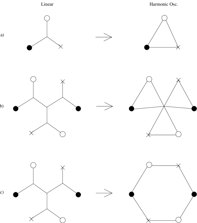
Figure 2.5: Different $\mathrm{SU}_{h}(3)$ flux-tube construction schemes (RHS) motivated by their corresponding linear cousins (LHS). Figures a) and c) represented the HP construction. Figures a) and b) show a construction scheme with a more consistent weighting for $s$-states.

The $\mathrm{SU}_{h}(2)$ model, by Watson [5], agrees with the HP model [4]. These graphs appear to be similar to those shown in figures 2.3 and 2.4. Of course the fact that these models agree is only a check of consistency, as they both have the same potential, which only includes interactions between $q\bar{q}$ pairs. Also the $\mathrm{SU}_{h}(2)$ models [4, 5] when compared with $\mathrm{SU}_{\ell}(2)$ [5] gives similar contrasting figures to the ones presented here.

Figure 2.4, along with similar figures given in references [4, 5], show a saturation of nuclear forces as $\rho\rightarrow\rho_{c}$, followed by a phase transition to quark matter at $\rho_{c}$. All of these models, however, fail to give any nuclear binding below $\rho_{c}$, which would seem to suggest that the flux-tube models are incapable of obtaining nuclear binding. Even the $\mathrm{SU}_{h}(3)$ HP model with its long chains, which tends to underestimate the potential, indicates that this would appear to be the case [4]. HP have a 2q model [4] that would seem to suggest that even if colour were not fixed to a given quark, no nuclear binding would occur: albeit this model is for $p$-wave (qq) states. Thus, it would appear that string-flip models, even those that include higher order flux-tube topologies, or allow the colour to move from quark to quark, are insufficient to obtain nuclear binding. Therefore, another mechanism for obtaining nuclear binding must be included in these models.

One possibility is to include one-gluon exchange interactions. As suggested by Nzar and Hoodbhoy [17], the most significant of these are the hyperfine interactions. In a relativistic setting one could also consider the possible effect of chiral symmetry breaking in which the constituent quark mass changes with momentum scale [28, 29]. Finally, other effects such as quark mass differences and isospin are expected to be negligible.

2.6 Conclusion

Various string-flip potential models have been discussed in general, and have been shown to adequately describe the bulk properties of nuclear/quark matter with the exception of nuclear binding. At low densities they yield free nucleon matter and at high densities a phase transition to free quark matter. They show an overall saturation of nuclear forces as nucleon densities are increased. At intermediate densities these models, with the exception of the HP $\mathrm{SU}_{h}(3)$ linked chain model [4], give an overall EMC-like swelling of the nucleon. It is believed that these models with the addition of one-gluon exchange effects should be capable of predicting nuclear binding. This is the topic of the next chapter.

Chapter 3 Flux-Bubble Models and Mesonic Molecules

3.1 Introduction

In the previous chapter string-flip potential models were investigated. It was hypothesized that these models by themselves were incapable of producing nuclear binding and would therefore have to be extended. The suggested extension was to include one-gluon exchange interactions. In this chapter a new class of models, called flux-bubble models, is proposed which allows for the extension of the flux-tube model to include these interactions.

3.2 Flux-Bubble Models

The primary objective is to construct a model which combines both nonperturbative (flux-tubes) and perturbative (one-gluon exchange) aspects of QCD in a consistent fashion. In order to simplify this task only the colour Coulomb extensions to an $SU_{\ell}(2)$ potential model will be considered.

The extension of the linear potential model for $q\bar{q}$ pairs is

where $\lambda_{ij}=-3/4,1/4$ for unlike and like colours respectively, and $\alpha_{s}\approx 0.1\,$. This is simply a variant of the phenomenological potential,

${\displaystyle V(r)\sim\sigma\,r-\frac{4}{3}\,\frac{\alpha_{s}}{r}\;}$, (1.1)

mentioned in chapter 1; the major difference being that the nonperturbative and perturbative parts are completely isolated in the former as opposed to the latter. When the quarks are separated at a distance greater than r₀ the potential is purely linear and when they are inside this radius it is purely Coulomb. In effect, for distances less than r₀, a “bubble” is formed in which the quarks are free to move around, in an asymptotically free fashion. In both distance regimes the net colour of the system is neutral.

The extension of the linear potential although simple for a pair of quarks becomes more complex when considering extensions for many pairs of quarks. In particular, how can a potential model be constructed in which some quarks are close enough to be inside perturbative bubbles while at the same time a subset of them are still connected to nonperturbative flux-tubes that extend outside of these bubbles. The solution to this problem is easily remedied by inserting virtual $q\bar{q}$ pairs across any of the intersection boundaries formed by the flux-tubes with the bubbles. Now the segments of flux-tubes that lie outside the bubbles remain intact while the segments inside simply dissolve; giving the desired result. Figure 3.1 illustrates the dynamics of this model.

Notice that this model allows the construction of colourless objects because of the insertion of the virtual $q\bar{q}$ pairs. These virtual quarks are used as a tool to calculate the overall length of the flux-tube correctly. They are not used in computing the Coulomb term however, as the field energy is already taken into account by the “real” quarks inside the bubbles. In general, once the bubbles have been determined, the flux-tubes must be reconfigured in order to minimize the linear part of the potential.

Although the model is currently for $SU_{\ell}(2)$ it should be easy to extend it to a full $SU_{\ell}(3)$ model with all the one-gluon exchange phenomena.

3.3 In Search of a Wave Function

Figure 3.2 shows some preliminary results using the $SU_{\ell}(2)$ flux-bubble model described in the previous section.

Figure 3.2: $E_{B}(\rho)$, (a), and $\beta(\rho)$, (b), for ${\rm r}_{0}=0\,$fm ($-\,-$) and ${\rm r}_{0}=0.1\,$fm(—), with $m_{q}=330MeV\,$, $\sigma=910MeV/fm\,$, and $\alpha_{s}=0.1\,$. These graphs were created by using a coarse $10\times 10$ mesh of points in $\rho$ and $\beta$. The minimal curves were extracted by using linear interpolation between the minimum data points on the $E_{B}(\rho,\beta)$-mesh surface.

For ${\rm r}_{0}=0\,fm$ the Monte Carlo recovers the same results for the $SU_{\ell}(2)$ string-flip potential model [5], as expected, and for ${\rm r}_{0}=0.1\,fm$ the result differs only slightly.

These results are questionable, as the wave function that was used is not ideal. It consisted of a slight modification to an old $SU_{\ell}(2)$ wave function [5],

$$\Psi_{\alpha\alpha^{\prime}\beta\rho}=\underbrace{\mathrm{e}^{-{\displaystyle\sum_{{\rm min}\{\mathrm{q\bar{q}}\}}(\beta r_{\rm q\bar{q}})^{\alpha}}}}_{\chi^{\rm(Linear)}_{\alpha\beta}}\,\Phi^{\rm(Fermi)}_{\rho}$$ (3.2)

(cf. equation 2.12), in which a new correlation piece, $\chi^{\rm(Coulomb)}_{\alpha^{\prime}\beta}\,$, was added to account for the local attractive Coulomb interactions as they occurred: i.e.,

$$\Psi_{\alpha\alpha^{\prime}\beta\rho}\;\sim\;\chi^{\rm(Linear)}_{\alpha\beta}\;\times\;\chi^{\rm(Coulomb)}_{\alpha^{\prime}\beta}\;\times\;\Phi^{\rm(Fermi)}_{\rho}\;,$$ (3.3)

where

$$\chi^{\rm(Coulomb)}_{\alpha^{\prime}\beta}=\mathrm{e}^{-{\displaystyle\sum_{\overline{{\rm min}\{{\rm q\bar{q}}\}}}\{(\beta r_{\rm q\bar{q}})^{\alpha^{\prime}}\theta(r_{0}-r_{\rm q\bar{q}})\}}}$$ (3.4)

with $\alpha=1.75$ and $\alpha^{\prime}=1\,$ (the repulsive interactions were assumed to be taken care of by the presence of the Slater wave function, $\Phi^{\rm(Fermi)}_{\rho}\,$). However, because the flux-tubes and bubbles can now be created or destroyed the wave function is, in general, no longer continuous to order $\vec{\nabla}^{2}$ (cf. equation 3.4), and so a variational lower bound is no longer guaranteed. Therefore, a new wave function is needed. Unfortunately, it is a rather difficult task to come up with a wave function that takes into account the locality of these flux-bubble interactions which is smooth and continuous, and involves very few parameters.

The aforementioned wave function has two “independent” parameters, $\rho$ and $\beta$; the $\alpha$’s were assumed to be fixed. This is in contrast to the previous case for the $SU_{\ell}(3)$ model, in chapter 2, in which $\rho$ and $\beta$ varied parametrically with a single parameter, $\theta\,$. The reason this does not apply here is because the flux-bubble potential breaks the scaling transformation

${\displaystyle(\beta,\rho^{1/3})\;\longrightarrow\;\zeta(\theta)\,(\cos\theta,\sin\theta)\,}$. (2.30)

This extra degree of freedom greatly increases the computation time.

The results in figure 3.2 were generated on a coarse $10\times 10$ mesh of points, in $\rho$ and $\beta$, and required 18hrs of CPU time on an 8 node farm. Clearly this procedure would be ridiculously slow if more parameters were to be added:

$$\tau_{\mbox{\tiny CPU}}\;\sim\;{\cal O}(R^{\vspace{1ex}p})$$ (3.5)

where $R$ is the mesh resolution in each ordinate, and $p$ is the number of parameters.

Therefore, a way of checking different wave functions and minimization schemes which does not consume large amounts of CPU time is desirable. In particular, a mini-laboratory is needed in which various aspects of the string-flip and flux-bubble potential models, from wave functions to minimization schemes, can be investigated.

3.4 Mesonic Molecules

Some work was done with mesonic-molecules [30] by Treurniet and Watson [31], using $SU_{\ell}(2)$, which has shown that these molecules make useful mini-laboratories for studying string-flip potential models. They used a mesonic-molecule, $Q_{2}$, consisting of two heavy quarks and two relatively light antiquarks: see figure 3.3.

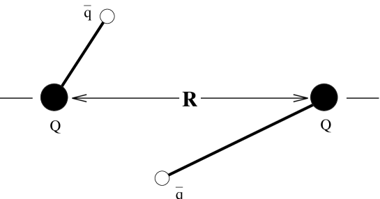
Figure 3.3: A mesonic-molecule, $Q_{2}\,$, with two heavy quarks and two light antiquarks.

The quarks are assumed to be heavy so that the light antiquarks can move around freely without disturbing their positions. By varying the distance, R, between the heavy quarks a mesonic-molecular potential, $U(R)\,$, can be computed (cf. equation 3.11). The $Q_{2}$ system provides a good way of checking potential models for the possibility of nuclear (mesonic) binding. Moreover, because of its simplicity, it allows for checking various wave functions and minimization schemes without being concerned about CPU overhead.

3.4.1 The Distributed Minimization Algorithm

There are many ways of determining the minimum of a function, $f(x)$, of several variables, $x=(x_{1}$,…,$x_{n})\,$ [32]. However, for the case where the function is approximated by Monte Carlo most of these methods, in general, will not work. The reason for this is because Monte Carlo calculations produce results that have statistical uncertainties; most of the methods are for functions that give “exact” answers. For example, if gradient methods were used, then the error would propagate into the gradient calculations which would effectively add noise to the search.

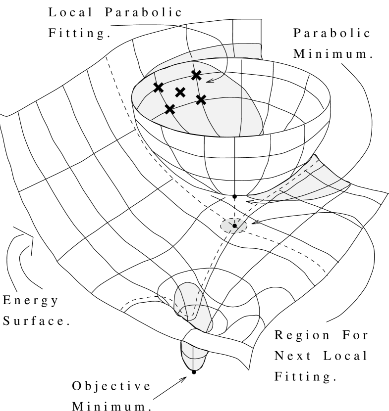
Figure 3.4: The parabolic minimization algorithm for an arbitrary $d$-dimensional, $d-D\,$, energy surface, where $p=\frac{1}{2}d(d-1)+2d+1$ is the minimum number of parameters required for fitting locally to a $d-D$ parabola.

Of the viable methods the most promising one is the parabolic minimization algorithm [33]. The algorithm is as follows (see figure 3.4):

• Pick an initial starting point, $x_{i}\,$.

• Pepper its neighborhood with $p$ points, $x_{p}\,$.

• Evaluate the $d-D$ function, $f(x)$, at these points.

• Fit a $d-D$ parabola to these evaluated points, $(f(x_{p,i}),x_{p,i})\,$.

• Find the critical point, $x_{c}\,$, of the parabola.

• Use this point to repeat the procedure.

This algorithm will, in general, converge to a critical point on the surface that is being searched. However, this does not guarantee that the point will be a minimum, it could very well be a maximum or a saddle point. Therefore, it is important to check the curvature [33] and then take appropriate measures to drive the search away from this point if is indeed not a minimum. Additionally, it is probably a good idea to bound the search to a box so that it does not drift out to infinity. It is important to note that this algorithm does not guarantee convergence to a global minimum but then neither does any other algorithm.

This algorithm must now be adapted to take advantage of a distributed computing environment.

The first step is simply to submit $p$ points to $m$ computers; where if $p<m$ use $p$ computers and if $p\geq m$ distribute $p/m$ jobs per computer (a slight improvement on this last step would be to distribute $m$ points and then dole out the remaining $m+i$ ($i$=1,…,$p-m$) points to the machines that finish first). However, this method is very inefficient because each iteration runs in time

$$\tau\sim{\cal O}(\left\lceil\frac{p}{m}\right\rceil)\,.$$ (3.6)

A much more efficient method would be to develop a procedure that analyzes the data in a continuous fashion as it streams in, point by point.

Such an algorithm was developed over the course of time that it took to produce the results in the later sections of this chapter. The details of the algorithm can be found in § B.2. A basic outline of the procedure is as follows:

1. Create an initial data base of $\kappa-m$ sample points, $(f(x_{\kappa-m}),x_{\kappa-m})\,$, with $m$ points pending.

2. Fit the neighborhood of each sample point to a parabola.

3. Submit the critical points, $x_{c}\,$, that correspond to parabolic minima.

4. Keep the $m$ computers occupied by submitting extra sampling points if necessary.

5. Wait for a point, $(f(x),x)\,$, to arrive.

6. Update the data base.

7. Fit the point about its neighborhood to a parabola.

8. Submit the newly predicted point, $x_{c}\,$, if it corresponds to a parabolic minimum.

9. Go back to step 4.

This algorithm is effectively performing several parabolic minimizations all on different regions of the $d-D$ surface $f(x)$ by interlacing its searches. For the work done here the convergence turned out to be quite rapid (due to cross-talking) with a fairly small start up cost,

$$\tau_{s}\sim{\cal O}(\left\lceil\frac{\kappa}{m}\right\rceil)\,,$$ (3.7)

where typically

$$\kappa\sim{\cal O}(2p)+m\,:$$ (3.8)

i.e., there were $m$ points pending at the time of creation of the data base in step 1, above. Also the time between iterations (i.e., “events”) was observed to be

$$\tau_{i}\sim{\cal O}(\frac{1}{m})\,,$$ (3.9)

where $m\leq 8\,$. Ultimately this algorithm will saturate when $\tau_{i}$ approaches the time required to process each calculation, $\tau_{p}\,$. $\tau_{p}$ is not a constant but a function of the size of the ever building data base and therefore will grow with time. Regardless though $\tau_{p}<<\tau_{i}$ and therefore for all practical purposes equation 3.9 holds. At some point $m$ will become large enough that this algorithm would begin to have the appearance of simple grid search. In fact, it was designed with this in mind.

For the Monte Carlo results contained herein the number of iterations required to obtain an accuracy well below the 1% level was about 30, 60, and 150 for the 1, 2, and 3 dimensional searches, respectively. Upon further investigation it was found that the convergence criterion that was used was too weak. The minimum was found after about 65% of the iterations needed to meet the convergence criterion. It is important to point out that this algorithm is still in its infancy and requires further development. Indeed, later work with the $1-D$ searches have reduced the iterations by about 50% and is expected to do the same for higher dimensional searches. The improvements were mainly due to establishing good convergence criterion and weighting techniques (see § B.2).

3.4.2 A General Survey of Extensions to $SU_{\ell}(2)$

In this section the effects of extending the old $SU_{\ell}(2)$ [5] model to include flux-bubbles, with and without fixed colour, will be investigated in the context of the mesonic-molecular system, $Q_{2}\,$. To simplify the situation these extensions will be considered in the frame work of $SU(2)$ colour, $SU_{c}(2)$.

A good place to start is by studying a $Q_{2}$ effective potential, $U(R)\,$, that was generated by interactions with the light antiquarks through a linear potential,

$$V=\sigma\,\sum_{\min\{Q\bar{q}\}}r_{Q\bar{q}}\,,$$ (3.10)

where the sum, ${\small\displaystyle\sum_{\min\{Q\bar{q}\}}}\,$, is over the set of quark-antiquark pairs, $\{Q\bar{q}\}\,$, which minimizes the potential, $r_{Q\bar{q}}$ represents the distance between a given light antiquark, $\bar{q}\,$, and a given – fixed – heavy quark, $Q\,$, and $\sigma\approx 910MeV/fm\,$. The Schrödinger equation that describes the effective potential between the two heavy quarks, in the adiabatic approximation, is as follows [34]

$$\left(\frac{1}{2m_{q}}\sum_{\bar{q}}\vec{\nabla}^{2}_{\bar{q}}+V\right)\Psi=U(R)\Psi\,,$$ (3.11)

with $m_{q}\approx 330MeV\,$. For the old $SU_{\ell}(2)$ model the variational wave function was assumed to be of the form [5],

$$\Psi_{\alpha\beta}=\mathrm{e}^{-{\displaystyle\sum_{\min\{Q\bar{q}\}}(\beta r_{Q\bar{q}})^{\alpha}}}\,.$$ (3.12)

Therefore, following a similar procedure to that of section 2.4 the effective potential is found by evaluating

$$\bar{U}=\bar{T}_{C}+\bar{V}$$ (3.13)

where

$$\bar{T}_{C}=\alpha\beta^{\alpha}\,\frac{1}{2m_{q}}\,\langle\sum_{\min\{Q\bar{q}\}}[\alpha(1-(\beta r_{Q\bar{q}})^{\alpha})+1]\,r_{Q\bar{q}}^{\alpha-2}\rangle\,,$$ (3.14)

(cf. equation 2.23), at different values of $R\,$.

Figure 3.5 shows a plot of the Monte Carlo results for $\bar{U}(R)$ where $\alpha$ and $\beta$ have both been allowed to vary.

Figure 3.5: The $Q_{2}$ potential obtained using a linear interaction with a pseudo-hydrogen wave function, equation 3.12.

This potential has been parameterized by a pseudo-Morse potential of the form

$$\tilde{U}(r)=\left\{e^{-2\eta[\beta(r-r_{0})]^{\alpha}}-2\eta e^{-[\beta(r-r_{0})]^{\alpha}}\right\}\,\tilde{\sigma}\,(r-r_{0}^{\prime})+\tilde{U}_{\infty}\,.$$ (3.15)

The term in the braces, “{}”, on the left along with $\tilde{\sigma}$ is the Morse potential [34, 35] with two extra parameters included; $\eta$ and $\alpha$. Outside the brackets to the right is a linear term with an offset parameter $r_{0}^{\prime}$ (this mainly takes effect in cases where the $Q_{2}$ potential blows up at the origin). Finally $\tilde{U}_{\infty}$ is the total energy at infinite separation. For these figures and the figures which follow, it will be assumed that $\eta=1$ and $r_{0}^{\prime}=0$ unless specified otherwise. A summary of the values of these parameters can be found in table 3.1. This parameterization was used mainly because it gave a fairly universal description of the (fully minimized) potentials in this chapter, however its physical significance should be taken lightly.

Table 3.1: Summary of parameters for the fits in figure 3.5.

Potential	Parameters
Pseudo-Morse	$\beta\;(fm^{-1})$	$r_{0}\;(fm)$	$\alpha$
	$1.162\pm 0.083$	$-0.41\pm 0.18$	$3.0\pm 1.2$
	$\tilde{\sigma}\;(MeV/fm)$	$\tilde{U}_{\infty}\;(MeV)$	$r_{0}^{\prime}\;(fm)$
	$11.9\pm 7.1$	$1709.4\pm 0.4$	$0.033\pm 0.060$
Yukawa	$V_{0}\;(MeV)$	$a\;(fm)$	$V_{\infty}\;(MeV)$
	$39.8\pm 3.2$	$0.3092\pm 0.0075$	$1709.40\pm 0.02$
Parabolic	${\cal C}\;(MeV/fm^{2})$	$r_{0}\;(fm)$	$y_{0}\;(MeV)$
	$32.6\pm 2.8$	$0.4060\pm 0.015$	$1706.2\pm 0.1$

The values of Monte Carlo results for $\bar{U}(R)$ at the end points of the curve, from $R=0fm$ and out to $R=5fm$, were checked against the analytic solution (cf. [5] and equation 2.29)

$$E_{free}=2\left(\frac{g_{T}^{\mbox{}}(\alpha)}{2\mu}\,\beta^{2}+g_{L}^{\mbox{}}(\alpha)\,\frac{\sigma}{\beta}\right)\,,$$ (3.16)

where

$$g_{T}^{\mbox{}}(\alpha) = \frac{\alpha^{2}\,\mbox{2\raisebox{6.45831pt}{$\frac{2}{\alpha}-2$}}\,\Gamma(2+1/\alpha)}{\Gamma(3/\alpha)}\,,$$ (3.17)

$$g_{L}^{\mbox{}}(\alpha) = \frac{\Gamma(4/\alpha)}{\mbox{2\raisebox{6.45831pt}{$\frac{1}{\alpha}$}}\,\Gamma(3/\alpha)}\,,$$ (3.18)

and $\mu$ ($\approx m_{q}$) is the reduced mass. This solution was easy to obtain because at the two extremes, $R=0$ and $R=\infty\,$, V becomes separable; the $Q_{2}$ system becomes equivalent to two isolated mesons. Equation 3.16 can be minimized in $\alpha$ and $\beta$ easily by using Mathematica [36]. The results can be found in table 3.9 of § 3.4.1.

It is interesting to investigate whether or not the string-flip potential, equation 3.10, actually mimics pion exchange. Therefore, the asymptotic part of $U(R)\,$, in figure 3.5, has been fitted to a Yukawa potential:

$$V(r)=-V_{0}\,\frac{e^{-r/a}}{r/a}\,+V_{\infty}\,,$$ (3.19)

and so the mass of the exchange particle is

$$\framebox{$\displaystyle m_{\mbox{\tiny ex}}=\frac{\hbar c}{a}$}\,.$$ (3.20)

A summary of the values of the parameters $V_{0}\,$, $a\,$, and $V_{\infty}$ can be found in table 3.1. Therefore,

$$m_{\mbox{\tiny ex}}\approx(638\pm 15)MeV\,,$$ (3.21)

which is about $4.6$ times too big.

Finally a test of whether or not the system is capable of binding can be done by expanding about the minimum of $\bar{U}(R)$ by using the parabolic approximation [35]

$$y(r)={\cal C}(r-r_{0})^{2}+y_{0}\,,$$ (3.22)

which can be transformed into the harmonic oscillator potential

$$V_{h}(r)=-D+\mbox{$\textstyle\frac{{1}}{{2}}$}\mu_{Q}\omega^{2}(r-r_{0})^{2}\,,$$ (3.23)

with

$$\framebox{$\displaystyle D=U_{\infty}-y_{0}$}\,,$$ (3.24)

$\omega=c\,\sqrt{2{\cal C}/\mu_{Q}}\,$, and $\mu_{Q}=m_{Q}/2\,$, where $U_{\infty}$ shall be taken as the analytic result for $U(R)$ out at $\infty$. Therefore, the binding energy is

$$E_{h}^{\nu}=-D+\hbar\omega(\nu+\mbox{$\textstyle\frac{{1}}{{2}}$})\,,$$ (3.25)

which implies

$$\framebox{$\displaystyle\mu_{Q}\geq\frac{{\cal C}(\hbar c)^{2}}{2(U_{\infty}-y_{0})^{2}}$}$$ (3.26)

in order to obtain binding. A summary of the parameters ${\cal C}\,$, $r_{0}\,$, and $y_{0}\,$, and the analytic result $U_{\infty}$ can be found in tables 3.1 and 3.9, respectively. So to obtain binding

$$\mu_{Q}\,\raisebox{-2.69096pt}{$\stackrel{{\scriptstyle>}}{{\sim}}$}\,(55\pm 6)GeV\,;$$ (3.27)

which is not surprising as the well is quite shallow,

$$D\approx(3.4\pm 0.1)MeV\,.$$ (3.28)

The next step is to add an $SU_{c}(2)$ term to the linear potential, equation 3.10,

$$V=\sum_{\min\{Q\bar{q}\}}\left[\sigma\,(r_{Q\bar{q}}-r_{0})\,\theta(r_{Q\bar{q}}-r_{0})-\frac{3}{4}\,\alpha_{s}\,\left(\frac{1}{r_{Q\bar{q}}}-\frac{1}{r_{0}}\right)\theta(r_{0}-r_{Q\bar{q}})\right]\,,$$ (3.29)

where $\alpha_{s}\approx 0.1\,$, and $r_{0}\approx 0.1fm\,$. Figure 3.6 shows the results of the Monte Carlo for this potential.

Figure 3.6: The $Q_{2}$ potential obtained using a linear-plus-coulomb interaction with a pseudo-hydrogen wave function.

The Monte Carlo results for $\bar{U}(R)$ were checked at $R=0fm$ and $R=5fm$ against the analytic solution

$$E_{free} = 2\left[\frac{g_{T}^{\mbox{}}(\alpha)}{2\mu}\,\beta^{2}+\sigma\left(\frac{g_{L}^{\mbox{}}(\alpha,\beta)}{\beta}-g_{0}^{\mbox{}}(\alpha,\beta)\,r_{0}\right)\right.$$ (3.30)

$$\left.-\frac{3}{4}\,\alpha_{s}\left(g_{C}^{\mbox{}}(\alpha,\beta)\,\beta-\frac{(1-g_{0}^{\mbox{}}(\alpha,\beta))}{r_{0}}\right)\right]\,,$$

where $g_{T}^{\mbox{}}(\alpha)$ is given by equation 3.17,

$$g_{L}^{\mbox{}}(\alpha,\beta) = \frac{\Gamma(4/\alpha,2(\beta r_{0})^{\alpha})}{\mbox{2\raisebox{6.45831pt}{$\frac{1}{\alpha}$}}\,\Gamma(3/\alpha)}\;\;\;\;\;\;\;\;\;\;\;\;\;\;\;\;=\;(1-{\rm P}(4/\alpha,2(\beta r_{0})^{\alpha})\,)\,g_{L}^{\mbox{}}(\alpha)\,,\;\;\;\mbox{}$$ (3.31)

$$g_{C}^{\mbox{}}(\alpha,\beta) = \frac{\Gamma(2/\alpha)-\Gamma(2/\alpha,2(\beta r_{0})^{\alpha})}{\mbox{2\raisebox{6.45831pt}{$-\frac{1}{\alpha}$}}\,\Gamma(3/\alpha)}\;=\;{\rm P}(2/\alpha,2(\beta r_{0})^{\alpha})\,g_{C}^{\mbox{}}(\alpha)\,,$$ (3.32)

$$g_{0}^{\mbox{}}(\alpha,\beta) = \frac{\Gamma(3/\alpha,2(\beta r_{0})^{\alpha})}{\Gamma(3/\alpha)}\;\;\;\;\;\;\;\;\;\;\;\;\;\;\;\;=\;1-{\rm P}(3/\alpha,2(\beta r_{0})^{\alpha})\,,$$ (3.33)

where $g_{L}^{\mbox{}}(\alpha)$ is given by equation 3.18,

$$g_{C}^{\mbox{}}(\alpha)=\frac{\Gamma(2/\alpha)}{\mbox{2\raisebox{6.45831pt}{$-\frac{1}{\alpha}$}}\,\Gamma(3/\alpha)}\,,$$ (3.34)

${\rm P}(a,z)=1-\Gamma(a,z)/\Gamma(a)\,$, and $\Gamma(a,z)$ is the incomplete gamma function [36, 37]. At $R=0fm$ and $R=5(\approx\infty)$ the system effectively decouples into two isolated mesons, for which equation 3.30 was derived. Notice that in the limits $r_{0}\rightarrow 0$ and $r_{0}\rightarrow\infty$ equation 3.30 simplifies to the earlier linear solution, equation 3.16, and to the Coulomb solution,

$$E_{free}\;\;\mbox{\raisebox{-2.58334pt}{$\stackrel{{\scriptstyle\longrightarrow}}{{\mbox{\tiny$r_{0}\rightarrow\infty$}}}$} }\;\;2\left(\frac{g_{T}^{\mbox{}}(\alpha)}{2\mu}\,\beta^{2}-\frac{3}{4}\,\alpha_{s}g_{C}^{\mbox{}}(\alpha)\,\beta\right)\,,$$ (3.35)

respectively. The analytic (i.e., the minimum of equation 3.30, via Mathematica [36]) verses the Monte Carlo results are summarized in table 3.2.

Table 3.2: Monte Carlo (MC) vs. analytic results for a linear-plus-coulomb potential.

Parameters		Analytic	MC @ $R=0fm$	MC @ $R=5fm$
$E_{min}(\alpha,\beta)$	$(MeV)$	1527.07	$1527.58\pm 0.04$	$1527.61\pm 0.05$
$\alpha$		1.74	1.74	1.72
$\beta$	$(fm^{-1})$	1.37	1.37	1.38

The results for the pseudo-Morse, Yukawa, and parabolic fits are summarized in table 3.3.

Table 3.3: Summary of parameters for the fits in figure 3.6.

Potential	Parameters
Pseudo-Morse	$\beta\;(fm^{-1})$	$r_{0}\;(fm)$	$\alpha$
	$2.01\pm 1.3$	$-0.01\pm 0.41$	$2.0\pm 1.3$
	$\tilde{\sigma}\;(MeV/fm)$	$\tilde{U}_{\infty}\;(MeV)$	$r_{0}^{\prime}\;(fm)$
	$11.2\pm 6.0$	$1527.6\pm 0.5$	$0.027\pm 0.072$
Yukawa	$V_{0}\;(MeV)$	$a\;(fm)$	$V_{\infty}\;(MeV)$
	$13.61\pm 0.55$	$0.4299\pm 0.0082$	$1527.70\pm 0.02$
Parabolic	${\cal C}\;(MeV/fm^{2})$	$r_{0}\;(fm)$	$y_{0}\;(MeV)$
	$33.1\pm 1.6$	$0.419\pm 0.053$	$1524.2\pm 0.1$

The Yukawa potential gives an exchange particle mass of

$$m_{\mbox{\tiny ex}}\approx(459\pm 4)MeV\,.$$ (3.36)

which is about $(3.3)$ times too big. The parabolic fit yields a well depth of

$$D\approx(2.9\pm 0.1)MeV$$ (3.37)

with the mass constraint

$$\mu_{Q}\,\raisebox{-2.69096pt}{$\stackrel{{\scriptstyle>}}{{\sim}}$}\,(77\pm 6)GeV\,,$$ (3.38)

in order to obtain binding.

Next the potential in equation 3.29 is extended to include all of the flux-bubble interactions, where the colour is fixed to each of the quarks:

$$V=\sigma\,\sum_{\min\{Q\bar{q}\}}(r_{Q\bar{q}}-r_{0})\,\theta(r_{Q\bar{q}}-r_{0})+\alpha_{s}\sum_{i<j}\lambda_{p_{i}p_{j}}\left(\frac{1}{r_{p_{i}p_{j}}}-\frac{1}{r_{0}}\right)\theta(r_{0}-r_{p_{i}p_{j}})\,,$$ (3.39)

with particle index $p_{k}\;\varepsilon\;\{Q_{i},\bar{q}_{j}|i,j=1,2\}\,$, such that $k=1,2,3,4\,$, and $SU_{c}(2)$ colour factor

$$\lambda_{p_{i}p_{j}}=\left\{\begin{array}[]{rl}-\frac{3}{4}&{\rm if}\;(p_{i},p_{j})\,\subseteq\,\{(\bar{q}_{i},Q_{j})\}\\ \frac{1}{4}&{\rm if}\;(p_{i},p_{j})\,\subseteq\,\{(\bar{q}_{i},\bar{q}_{j}),(Q_{i},Q_{j})\}\end{array}\right.\,.$$ (3.40)

Notice that V can be rewritten so that its extension to equation 3.29 is more apparent:

$$V = \sum_{\min\{Q\bar{q}\}}\left[\sigma\,(r_{Q\bar{q}}-r_{0})\,\theta(r_{Q\bar{q}}-r_{0})-\frac{3}{4}\,\alpha_{s}\,\left(\frac{1}{r_{Q\bar{q}}}-\frac{1}{r_{0}}\right)\theta(r_{0}-r_{Q\bar{q}})\right]$$ (3.41)

$$+\,\alpha_{s}\sum_{p_{i}p_{j}\,\varepsilon\,\overline{\min\{Q\bar{q}\}}}\lambda_{p_{i}p_{j}}\left(\frac{1}{r_{p_{i}p_{j}}}-\frac{1}{r_{0}}\right)\theta(r_{0}-r_{p_{i}p_{j}})\,,$$

where $\overline{\min\{Q\bar{q}\}}$ is the complement of the set $\min\{Q\bar{q}\}\,$, and therefore defining more precisely the sum in the exponent of the variational wave function, equation 3.12. Figure 3.7 shows the results of the Monte Carlo for this potential.

Figure 3.7: The $Q_{2}$ potential obtained using the flux-bubble interaction with a pseudo-hydrogen wave function.

The Monte Carlo results were checked against the analytic solution given by equation 3.30 at $R=5fm$ only, since the system no longer decouples at the origin. The results are summarized in table 3.4.

Table 3.4: Monte Carlo (MC) vs. analytic results for a flux-bubble potential.

Parameters		Analytic	MC @ $R=5fm$
$E_{min}(\alpha,\beta)$	$(MeV)$	1527.07	$1527.66\pm 0.05$
$\alpha$		1.74	1.71
$\beta$	$(fm^{-1})$	1.37	1.38

An attempt was made to fit $U(R)$ to the Morse potential [34, 35],

$$U_{M}(r)=U_{0}(e^{-2\beta(r-r_{0})}-2e^{-\beta(r-r_{0})})+U_{\infty}\,,$$ (3.42)

with binding energy

$$E^{\nu}_{M}=-D+\hbar\omega\left\{(\nu+\mbox{$\textstyle\frac{{1}}{{2}}$})-\frac{\beta\hbar c}{2\sqrt{2\mu_{Q}D}}(\nu+\mbox{$\textstyle\frac{{1}}{{2}}$})^{2}\right\}\,,$$ (3.43)

and depth $D=U_{0}\,$, where $\omega=\beta c\,\sqrt{2D/\mu_{Q}}\,$. For this potential

$$\mu_{Q}\geq\frac{(\beta\hbar c)^{2}}{8U_{0}}\,$$ (3.44)

is the corresponding binding constraint.

Table 3.5: Summary of parameters for the fits in figure 3.7.

Potential	Parameters
Pseudo-Morse	$\beta\;(fm^{-1})$	$r_{0}\;(fm)$	$\alpha$
	$1.34\pm 0.20$	$-0.63\pm 0.19$	$2.10\pm 0.37$
	$\tilde{\sigma}\;(MeV/fm)$	$\tilde{U}_{\infty}\;(MeV)$	$r_{0}^{\prime}\;(fm)$
	$40\pm 15$	$1527.6\pm 0.5$	$0.088\pm 0.031$
Yukawa	$V_{0}\;(MeV)$	$a\;(fm)$	$V_{\infty}\;(MeV)$
	$9.16\pm 0.42$	$0.498\pm 0.012$	$1527.70\pm 0.02$
Parabolic	${\cal C}\;(MeV/fm^{2})$	$r_{0}\;(fm)$	$y_{0}\;(MeV)$
	$31.7\pm 1.4$	$0.4042\pm 0.0044$	$1524.3\pm 0.1$
Morse	$\beta\;(fm^{-1})$	$r_{0}\;(fm)$	$U_{0}\;(MeV)$
	$2.62\pm 0.38$	$0.333\pm 0.039$	$3.09\pm 0.73$
	$U_{\infty}\;(MeV)$
	$1527.8\pm 0.5$

Table 3.5 contains a summary of the fits for the various potentials. The Morse and parabolic fits give,

$$(\mu_{Q})_{\mbox{\tiny Morse}}\;\;\; \stackrel{{\scriptstyle>}}{{\sim}} (11\pm 4)GeV\,,$$ (3.45)

$$(\mu_{Q})_{\mbox{\tiny parabolic}} \stackrel{{\scriptstyle>}}{{\sim}} (79\pm 7)GeV\,$$ (3.46)

with well depths

$$(D)_{\mbox{\tiny Morse}}\;\;\; \approx (3.1\pm 0.7)MeV\,,$$ (3.47)

$$(D)_{\mbox{\tiny parabolic}} \approx (2.8\pm 0.1)MeV\,.$$ (3.48)

Although the Morse gives a lower value it is a rather dubious one since the fit did not describe the shape of the knee or the minimum of the potential (see Morse fitting insert in figure 3.7) very well. Regardless, there is no binding.

Referring to equation 3.20 and to table 3.5 yields an exchange mass of

$$m_{\mbox{\tiny ex}}\approx{\cal O}(396\pm 10)MeV\,,$$ (3.49)

which is ${\cal O}(2.8)$ times too big.

Finally the flux-bubble potential is extended to allow the colour to move around. The potential is similar to that of equation 3.39 except that now the particle indices, $p_{k}$, carry colour degrees of freedom,

$$V = \sum_{\min\{q_{i}\bar{q}_{j}\}}\left[\sigma\,(r_{q_{i}\bar{q}_{j}}-r_{0})\,\theta(r_{q_{i}\bar{q}_{j}}-r_{0})-\frac{3}{4}\,\alpha_{s}\,\left(\frac{1}{r_{q_{i}\bar{q}_{j}}}-\frac{1}{r_{0}}\right)\theta(r_{0}-r_{q_{i}\bar{q}_{j}})\right]$$ (3.50)

$$+\,\alpha_{s}\sum_{p_{i}p_{j}\,\varepsilon\,\overline{\min\{q_{i}\bar{q}_{j}\}}}\lambda_{p_{i}p_{j}}\left(\frac{1}{r_{p_{i}p_{j}}}-\frac{1}{r_{0}}\right)\theta(r_{0}-r_{p_{i}p_{j}})\,,$$

where $\lambda_{p_{i}p_{j}}$ is defined just below equation 3.1, and

$$q_{k} \varepsilon \{R_{i},\bar{B}_{i},r_{i},\bar{b}_{i}|i=1,2\}\;\subseteq\;SU_{c}(2)\,,$$ (3.51)

$$\bar{q}_{k} \varepsilon \{\bar{R}_{i},B_{i},\bar{r}_{i},b_{i}|i=1,2\}\;\subseteq\;\overline{SU_{c}(2)}\,,$$ (3.52)

i.e., $b\;\sim\;\bar{r}\,,\,\mbox{\ldots, etc.}\;\;\Leftrightarrow\;\;SU_{c}(2)\;\sim\;\overline{SU_{c}(2)}\,,\;\;\;\;\;\;$
where the capital case letters are for the heavy quarks, the lower case letters are for the light quarks, the letters $r$ and $R$ represent the red quarks, and the letters $b$ and $B$ stand for the blue quarks. A further expansion of V leads to the more useful form

$$V = \sum_{\min\{q_{i}\bar{q}_{j}\}}\left[\sigma\,(r_{q_{i}\bar{q}_{j}}-r_{0})\,\theta(r_{q_{i}\bar{q}_{j}}-r_{0})-\frac{3}{4}\,\alpha_{s}\,\left(\frac{1}{r_{q_{i}\bar{q}_{j}}}-\frac{1}{r_{0}}\right)\theta(r_{0}-r_{q_{i}\bar{q}_{j}})\right]$$ (3.53)

$$-\frac{3}{4}\,\alpha_{s}\sum_{q_{i}\bar{q}_{j}\,\varepsilon\,\overline{\min\{q_{i}\bar{q}_{j}\}}_{+}}\left(\frac{1}{r_{q_{i}\bar{q}_{j}}}-\frac{1}{r_{0}}\right)\theta(r_{0}-r_{q_{i}\bar{q}_{j}})$$

$$+\frac{1}{4}\,\alpha_{s}\sum_{q_{i}q_{j}\,\varepsilon\,\overline{\min\{q_{i}\bar{q}_{j}\}}_{-}}\left(\frac{1}{r_{q_{i}q_{j}}}-\frac{1}{r_{0}}\right)\theta(r_{0}-r_{q_{i}q_{j}})\,,$$

where

$$\overline{\min\{q_{i}\bar{q}_{j}\}}=\overline{\min\{q_{i}\bar{q}_{j}\}}_{+}\cup\overline{\min\{q_{i}\bar{q}_{j}\}}_{-}\,,$$

plus, “+”, means attractive, and minus, “-”, means repulsive. Figure 3.8 shows the results of the Monte Carlo for this potential.

Figure 3.8: The $Q_{2}$ potential obtained using the full flux-bubble interaction, in which the colour is allowed to move around, with a pseudo-hydrogen wave function.

The Monte Carlo results were checked against the analytic solution given by equation 3.39 at $R=5fm$ ($\approx\infty$). The results are summarized in table 3.6.

Table 3.6: Monte Carlo (MC) vs. analytic results for a flux-bubble potential.

Parameters		Analytic	MC @ $R=5fm$
$E_{min}(\alpha,\beta)$	$(MeV)$	1527.07	$1527.62\pm 0.04$
$\alpha$		1.74	1.73
$\beta$	$(fm^{-1})$	1.37	1.37

Table 3.7 gives a summary of the global and local fits to the potential.

Table 3.7: Summary of parameters for the fits in figure 3.8.

Potential	Parameters
Linear	$m\;(MeV/fm)$	$r_{0}\;(fm)$	$b\;(MeV)$
	$910.0\pm 1.0$	$-1.5706\pm 0.0047$	$-534.6\pm 4.2$
Pseudo-Morse	$\beta\;(fm^{-1})$	$r_{0}\;(fm)$	$\alpha$
	$0.18834\pm 0.00033$	$-4.423\pm 0.012$	$11.29\pm 0.093$
	$\tilde{\sigma}\;(MeV/fm)$	$\tilde{U}_{\infty}\;(MeV)$	$r_{0}^{\prime}\;(fm)$
	$-1310.2\pm 5.5$	$1524.8\pm 0.5$	$0.6470\pm 0.0011$
	$\eta$
	$0.9447\pm 0.0024$

One of the most noticeable peculiarities of figure 3.8 is the apparent linearity of the inside of the potential. In fact, a linear fit to

$$y(r)=m(r-r_{0})+b$$ (3.54)

in this region (see the insert in figure 3.8 and the fitted results in table 3.7) yields a slope of $m\approx 910.0MeV/fm\,$! This corresponds to the linear potential $U\sim\sigma R\,$. A more subtle feature is at the origin (see the “blow up” insert in figure 3.8) where the potential starts to plummet to $-\infty$. This region is due to the coulomb attraction between the two heavy quarks. Out near $R=1fm$ there appears to be a barrier and beyond this no more structure. Therefore, as two mesons, each containing a heavy quark and a light anti-quark, are brought together from infinity they feel a repulsive force. When near enough, flux-tubes are exchanged, and the two mesons dissociate into one meson containing two heavy quarks and another containing two light anti-quarks. This situation shows that $SU_{c}(2)\,$, with moving colour, does not make a good model of nuclear matter.

Table 3.8 gives a summary of all the properties of the $Q_{2}$ potential for the linear, linear-plus-Coulomb, and flux-bubble (with fix colour) models that were studied in this section.

Table 3.8: Summary of the properties of $U(R)$.

		Fig. 3.5	Fig. 3.6	Fig. 3.7
$D$	$(MeV)$	$3.4\pm 0.1$	$2.9\pm 0.1$	$2.8\pm 0.1$
$\mu_{\mbox{\tiny min}}$	$(GeV)$	$55\pm 6$	$77\pm 6$	$79\pm 7$
$m_{\tiny ex}$	$(MeV)$	$638\pm 15$	$459\pm 4$	$396\pm 10$

In general the extensions of the basic linear potential model to include the colour-Coulomb interactions did not alter the $Q_{2}$ potential significantly enough to achieve binding. In fact, it only exacerbated the problem. However, these extensions did lead to a slight softening of the potential which perhaps suggests that there might be more to meson exchange than just flux-tube swapping. When the colour was allowed to move around a rather unphysical situation occurred which suggested that there was perhaps a problem with using $SU_{c}(2)$ or with the variational wave function itself — perhaps even both. In the next section a more detailed study of the properties of the wave function is carried out.

3.4.3 Back to the $SU_{\ell}(2)$ String-Flip Potential Model

When the $SU_{\ell}(2)$ string-flip potential model was investigated [5] the parameter $\alpha$ in the variational wave function, given in equation 3.2, was fixed by requiring that it minimize the total energy at zero density. Since this could be done analytically it allowed for a reduction in the number of variational parameters used in the Monte Carlo. It was assumed that the constraint would have very little affect on the physics as a function of density since the results varied by about 1% for $1.5\,<\,\alpha\,<2.1\,$, at zero density. The validity of this claim can now be checked more thoroughly by using the $Q_{2}$ mini-laboratory.

Figure 3.9 shows a plot of the Monte Carlo results, obtained via equations 3.10 3.12 and 3.13, for $\bar{U}(R)$ where $\alpha$ is allowed to vary, $\alpha=2.00\,$, and $\alpha=1.74\,$.

Figure 3.9: $\bar{U}(R)$ where $\alpha$ is, allowed to vary, fixed at 2, and fixed at 1.74. These potentials were found by minimizing $\langle U(R)\rangle_{\alpha,\beta}\,$, for fixed values of $R$, using the distributed minimization algorithm (§ 3.4.1). The $\langle U(R)\rangle_{\alpha,\beta}\,$, were evaluated using the Metropolis algorithm (§ 2.4).

$\alpha=2.00\,$ was the value used in the old $SU_{\ell}(2)$ model [5], and $\alpha\approx 1.74$ was the value that minimized $\bar{U}(R)$ at zero separation. The values of $\bar{U}(R)$ at the end points of the curves, from $R=0fm$ and out to $R=5fm$, were checked against the analytic solution given by equation 2.29 and have been tabulated in Table 3.9.

Table 3.9: Monte Carlo (MC) vs. analytic results for the $SU_{\ell}(2)$ $Q_{2}$-potential.

Parameters		Analytic	MC @ $R=0fm$	MC @ $R=5fm$
$E_{min}(\alpha,\beta)$	$(MeV)$	1709.61	$1709.42\pm 0.04$	$1709.49\pm 0.04$
$\alpha$		1.75	1.74	1.72
$\beta$	$(fm^{-1})$	1.37	1.37	1.38
$E_{min}(2.00,\beta)$	$(MeV)$	1714.38	$1714.83\pm 0.13$	$1714.72\pm 0.12$
$\beta$ @ $\alpha=2.00$	$(fm^{-1})$	1.27	1.25	1.28
$E_{min}(1.74,\beta)$	$(MeV)$	1709.62	$1709.43\pm 0.04$	$1709.43\pm 0.04$
$\beta$ @ $\alpha\approx 1.74$	$(fm^{-1})$	1.37	1.38	1.38

Figure 3.10 shows the variations in $\alpha\,$ and $\beta$ as a function of $R$.

Figure 3.10: Graph of $\alpha(R)$ & $\beta(R)$ for the $SU_{\ell}(2)$ $Q_{2}$-potential model. The dashed lines are for $\alpha=2.00$ and $\alpha\approx 1.74$. The noise is mainly due to shallow minima on the energy surfaces, $\bar{U}(R)$. The curve on the upper plot and the two upper curves on the lower plot have been parameterized by $a\,e^{-b\,R}\,R^{c}\,$, which are provided to guide the eye; they have no physical significance.

It would appear from this figure that when $\alpha$ is left free to vary, $\alpha$ and $\beta$ become extremely correlated. Regardless, looking at the maximum fluctuations about the central values of the parameters $\alpha\,$, $\beta\,$, and $U(R)\,$, from the information given in tables 3.10 and 3.1, $\alpha\approx(1.88\pm 0.13)\,$, $\beta\approx(1.32\pm 0.05)fm\,$, and $\langle\bar{U}(R)\rangle_{R}\approx(1710\pm 4)MeV$ which is certainly less then a 1% effect in the energy [5]. However for $\beta$ it would appear to be an ${\cal O}(4)$% effect which may have a slight affect on the rate of nuclear swelling.

Surprisingly the $\bar{U}(R)|_{\alpha=2}\,$ gives a much deeper well than expected if $\alpha$ was left as a free parameter: i.e., $D\approx{\cal O}(8)MeV\,$, via table 3.10. However, this well is not deep enough to give binding: i.e., a parabolic approximation about the minimum requires $\mu_{Q}\geq{\cal O}(15)GeV\,$, via equation 3.26 and table 3.10. For equal mass constituent quarks this is expected to be a much graver situation.

Table 3.10: Summary of the parameters used in the fits for the $\alpha=2$ curve in figure 3.9. See equations 3.15 and 3.22 for the definitions of these parameters.

Potential	Parameters
Parabolic	${\cal C}\;(MeV/fm^{2})$	$r_{0}\;(fm)$	$y_{0}\;(MeV)$
	$49.9\pm 3.5$	$0.3944\pm 0.0046$	$1706.7\pm 0.1$
Pseudo-Morse	$\beta\;(fm^{-1})$	$r_{0}\;(fm)$	$\alpha$
	$1.062\pm 0.013$	$-0.607\pm 0.016$	$2.768\pm 0.044$
	$\tilde{\sigma}\;(MeV/fm)$	$\tilde{U}_{\infty}\;(MeV)$
	$39.68\pm 0.87$	$1714.70\pm 0.04$

For certain fixed values of $\alpha\,$, $\alpha\approx 1.74$ in figure 3.9 for example, the potential gives a slight short range repulsion. For the range of $\alpha$ values being considered here it is well inside the potential. However, for values of $\alpha\approx 1.0$ the effect becomes quite dramatic.

In general, it is fairly safe to assume that the predicted outcome of the results of past papers [5, 9] will not change significantly if $\alpha$ is allowed to vary. However, because the wave function appears to be correlated in both $\alpha$ and $\beta\,$, this seems to suggest that another wave function should be considered in these models.

3.4.4 A New Wave Function

Wave functions for the old $SU_{\ell}(2)$ string-flip potential models have been examined. For the analysis based on the $Q_{2}$ system there appeared to be something pathological about the wave function that was used in these models. Further, despite this shortcoming, it was thought that this would not have any significant effect on the outcome of the physics predicted by past models. However, the purpose of using the $Q_{2}$ system was not only to study the properties of this wave function but to ascertain the possibility of devising a wave function with very few parameters that would take into account the locality of the flux-bubble interactions.

An interesting place to look for such a wave function is in the similarity between the $Q_{2}$ mesonic-molecular system and $H_{2}$ molecular system. Recall that the key reason for the atomic binding is the screening effect caused by the electrons which are for the most part “localized” in between the protons. This localization is achieved by using a variational wave function that was the superposition of the direct product of two ground state hydrogen atoms, [34, 38]

$$\Psi\sim\mbox{$e$\raisebox{8.61108pt}{$\displaystyle{-\beta(r_{e_{1}P_{1}}+r_{e_{2}P_{2}})}$}}+\mbox{$e$\raisebox{8.61108pt}{$\displaystyle{-\beta(r_{e_{2}P_{1}}+r_{e_{1}P_{2}})}$}}\,.$$ (3.55)

Although the $Q_{2}$ system is far removed from its $H_{2}$ cousin from a dynamical point of view, and the motivations for achieving localization are quite different, this variational wave function does solve the problem for the $H_{2}$ system. Therefore, it would seem plausible to make the following $ansatz$:

$$\Psi_{\alpha,\beta}=\mbox{$e$\raisebox{8.61108pt}{$\displaystyle{-\beta^{\alpha}(r_{\bar{q}_{1}Q_{1}}^{\alpha}+r_{\bar{q}_{2}Q_{2}}^{\alpha})}$}}+\mbox{$e$\raisebox{8.61108pt}{$\displaystyle{-\beta^{\alpha}(r_{\bar{q}_{2}Q_{1}}^{\alpha}+r_{\bar{q}_{1}Q_{2}}^{\alpha})}$}}\,.$$ (3.56)

If $\bar{q}_{1}Q_{1}$ and $\bar{q}_{2}Q_{2}$ represent two separate mesons then the first term represents the internal meson interactions while the second term represents the external meson interactions. Notice that the external interactions shut off as the separation, $R\,$, between the two heavy quarks becomes large,

$$\lim_{R\rightarrow\infty}\bar{\Psi}(R)=\mbox{$e$\raisebox{8.61108pt}{$\displaystyle{-\beta^{\alpha}(r_{\bar{q}_{1}Q_{1}}^{\alpha}+r_{\bar{q}_{2}Q_{2}}^{\alpha})}$}}$$ (3.57)

which is the desired property.

Using equation 3.11 and equation 3.57 the kinetic energy contribution to the effective potential $U(R)$ in equation 3.13 now becomes,

$$\bar{T} = 2\,\bar{T}_{-s}-\bar{F}^{2}$$ (3.59)

$$= \frac{\alpha\beta^{\alpha}}{2m_{q}}\left\langle\{[(\alpha+1)\,(r_{\bar{q}_{1}Q_{1}}^{\alpha-2}+r_{\bar{q}_{2}Q_{2}}^{\alpha-2})-\alpha\beta^{\alpha}\,(r_{\bar{q}_{1}Q_{1}}^{2\alpha-2}+r_{\bar{q}_{2}Q_{2}}^{2\alpha-2})]\,\mbox{$e$\raisebox{8.61108pt}{$\displaystyle{-2\beta^{\alpha}(r_{\bar{q}_{1}Q_{1}}^{\alpha}+r_{\bar{q}_{2}Q_{2}}^{\alpha})}$}}\right.$$

$$+\,[(\alpha+1)\,(r_{\bar{q}_{2}Q_{1}}^{\alpha-2}+r_{\bar{q}_{1}Q_{2}}^{\alpha-2})-\alpha\beta^{\alpha}\,(r_{\bar{q}_{2}Q_{1}}^{2\alpha-2}+r_{\bar{q}_{1}Q_{2}}^{2\alpha-2})]\,\mbox{$e$\raisebox{8.61108pt}{$\displaystyle{-2\beta^{\alpha}(r_{\bar{q}_{2}Q_{1}}^{\alpha}+r_{\bar{q}_{1}Q_{2}}^{\alpha})}$}}$$

$$+\,[(\alpha+1)\,(r_{\bar{q}_{1}Q_{1}}^{\alpha-2}+r_{\bar{q}_{2}Q_{2}}^{\alpha-2}+r_{\bar{q}_{2}Q_{1}}^{\alpha-2}+r_{\bar{q}_{1}Q_{2}}^{\alpha-2})$$

$$-\alpha\beta^{\alpha}\,(r_{\bar{q}_{1}Q_{1}}^{2\alpha-2}+r_{\bar{q}_{2}Q_{2}}^{2\alpha-2}+r_{\bar{q}_{2}Q_{1}}^{2\alpha-2}+r_{\bar{q}_{1}Q_{2}}^{2\alpha-2})]$$

$$\left.\times\mbox{$e$\raisebox{8.61108pt}{$\displaystyle{-\beta^{\alpha}(r_{\bar{q}_{1}Q_{1}}^{\alpha}+r_{\bar{q}_{2}Q_{1}}^{\alpha}+r_{\bar{q}_{1}Q_{2}}^{\alpha}+r_{\bar{q}_{2}Q_{2}}^{\alpha})}$}}\}/\Psi^{2}\right\rangle\,,$$

where

$$\bar{T}_{-s} = \frac{-1}{4m_{q}}\sum_{\bar{q}}\nabla_{\bar{q}}^{2}\ln\Psi$$

$$= \frac{\alpha\beta^{\alpha}}{4m_{q}}\left\langle\frac{(\alpha+1)}{\Psi}\left[(r_{\bar{q}_{1}Q_{1}}^{\alpha-2}+r_{\bar{q}_{2}Q_{2}}^{\alpha-2})\,\mbox{$e$\raisebox{8.61108pt}{$\displaystyle{-\beta^{\alpha}(r_{\bar{q}_{1}Q_{1}}^{\alpha}+r_{\bar{q}_{2}Q_{2}}^{\alpha})}$}}\right.\right.$$

$$\left.+\,(r_{\bar{q}_{2}Q_{1}}^{\alpha-2}+r_{\bar{q}_{1}Q_{2}}^{\alpha-2})\,\mbox{$e$\raisebox{8.61108pt}{$\displaystyle{-\beta^{\alpha}(r_{\bar{q}_{2}Q_{1}}^{\alpha}+r_{\bar{q}_{1}Q_{2}}^{\alpha})}$}}\right]$$

$$+\,\frac{\alpha\beta^{\alpha}}{\Psi^{2}}\,[(r_{\bar{q}_{1}Q_{1}}^{2}+r_{\bar{q}_{1}Q_{2}}^{2}-R^{2})\,r_{\bar{q}_{1}Q_{1}}^{\alpha-2}\,r_{\bar{q}_{1}Q_{2}}^{\alpha-2}+(r_{\bar{q}_{2}Q_{1}}^{2}+r_{\bar{q}_{2}Q_{2}}^{2}-R^{2})\,r_{\bar{q}_{2}Q_{1}}^{\alpha-2}\,r_{\bar{q}_{2}Q_{2}}^{\alpha-2}$$

$$\left.-\,(r_{\bar{q}_{1}Q_{1}}^{2\alpha-2}+r_{\bar{q}_{2}Q_{2}}^{2\alpha-2}+r_{\bar{q}_{2}Q_{1}}^{2\alpha-2}+r_{\bar{q}_{1}Q_{2}}^{2\alpha-2})]\,\mbox{$e$\raisebox{8.61108pt}{$\displaystyle{-\beta^{\alpha}(r_{\bar{q}_{1}Q_{1}}^{\alpha}+r_{\bar{q}_{2}Q_{1}}^{\alpha}+r_{\bar{q}_{1}Q_{2}}^{\alpha}+r_{\bar{q}_{2}Q_{2}}^{\alpha})}$}}\right\rangle\,,$$

and

$$\bar{F}^{2} = \frac{1}{2m_{q}}\sum_{\bar{q}}(\nabla_{\bar{q}}\ln\Psi)^{2}$$ (3.63)

$$= \frac{\alpha^{2}\beta^{2\alpha}}{2m_{q}}\left\langle\frac{1}{\Psi^{2}}\,\left[(r_{\bar{q}_{1}Q_{1}}^{2\alpha-2}+r_{\bar{q}_{2}Q_{2}}^{2\alpha-2})\,\mbox{$e$\raisebox{8.61108pt}{$\displaystyle{-2\beta^{\alpha}(r_{\bar{q}_{1}Q_{1}}^{\alpha}+r_{\bar{q}_{2}Q_{2}}^{\alpha})}$}}\right.\right.$$

$$\left.+\,(r_{\bar{q}_{2}Q_{1}}^{2\alpha-2}+r_{\bar{q}_{1}Q_{2}}^{2\alpha-2})\,\mbox{$e$\raisebox{8.61108pt}{$\displaystyle{-2\beta^{\alpha}(r_{\bar{q}_{2}Q_{1}}^{\alpha}+r_{\bar{q}_{1}Q_{2}}^{\alpha})}$}}\right]$$

$$+\,[(r_{\bar{q}_{1}Q_{1}}^{2}+r_{\bar{q}_{1}Q_{2}}^{2}-R^{2})\,r_{\bar{q}_{1}Q_{1}}^{\alpha-2}\,r_{\bar{q}_{1}Q_{2}}^{\alpha-2}+(r_{\bar{q}_{2}Q_{1}}^{2}+r_{\bar{q}_{2}Q_{2}}^{2}-R^{2})\,r_{\bar{q}_{2}Q_{1}}^{\alpha-2}\,r_{\bar{q}_{2}Q_{2}}^{\alpha-2}]$$

$$\left.\times\mbox{$e$\raisebox{8.61108pt}{$\displaystyle{-\beta^{\alpha}(r_{\bar{q}_{1}Q_{1}}^{\alpha}+r_{\bar{q}_{2}Q_{1}}^{\alpha}+r_{\bar{q}_{1}Q_{2}}^{\alpha}+r_{\bar{q}_{2}Q_{2}}^{\alpha})}$}}\right\rangle\,.$$

It is interesting to note, and it also serves as a good check of the computation, that in the large $R$ limit the kinetic energy corresponds exactly to the kinetic energy for the old wave function in the same limit:

$$\lim_{R\rightarrow\infty}\bar{T}(R) = \frac{\alpha\beta^{\alpha}}{2m_{q}}\left\langle(\alpha+1)\,(r_{\bar{q}_{1}Q_{1}}^{\alpha-2}+r_{\bar{q}_{2}Q_{2}}^{\alpha-2})-\alpha\beta^{\alpha}\,(r_{\bar{q}_{1}Q_{1}}^{2\alpha-2}+r_{\bar{q}_{2}Q_{2}}^{2\alpha-2})\right\rangle$$ (3.64)

$$= \frac{\alpha\beta^{\alpha}}{2m_{q}}\left\langle\sum_{i=1}^{2}[\alpha(1-(\beta r_{\bar{q}_{i}Q_{i}})^{\alpha})+1]\,r_{\bar{q}_{i}Q_{i}}^{\alpha-2}]\right\rangle\,,$$

cf. equation 3.14. Also direct evaluation of the RHS leads to (assuming $\Psi$ is properly normalized)

$$\lim_{R\rightarrow\infty}\bar{T}(R)=\frac{g_{T}(\alpha)}{m_{q}}\,\beta^{2}\,,$$ (3.65)

which is just the kinetic term for the analytic solutions given in equations 3.16 and 3.30.

The Monte Carlo computations that were done, using the pseudo-hydrogen wave function, $\tilde{\Psi}_{H}$ (equation 3.12) in § 3.4.2, have been repeated here for the pseudo-hydrogen-molecular wave function, $\tilde{\Psi}_{H_{2}}$ (equation 3.56), and are shown in figures 3.11 through 3.14. Table 3.3 contains a summary of the fits for these figures, table 3.12 contains a summary of the checks done against the analytic results and table 3.13 contains a summary of the properties of $U(R)\,$.

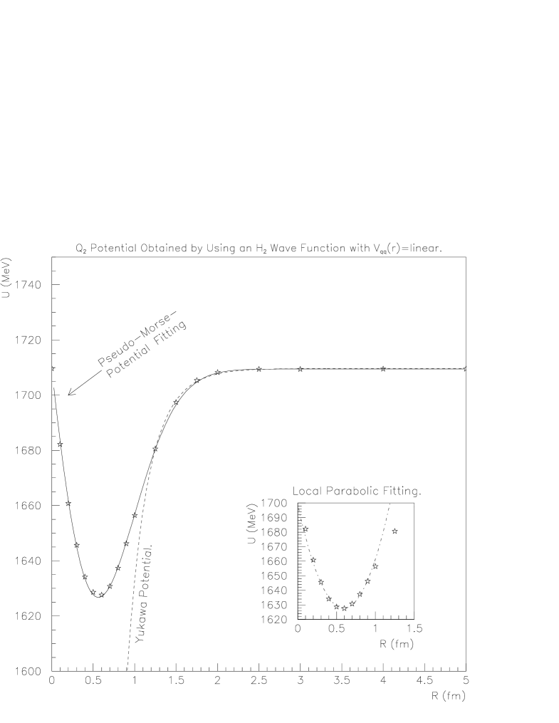
Figure 3.11: The $Q_{2}$ potential obtained using a linear interaction with $\tilde{\Psi}_{H_{2}}\,$.

Figure 3.12: The $Q_{2}$ potential obtained using a linear-plus-Coulomb interaction with $\tilde{\Psi}_{H_{2}}\,$.

Figure 3.13: The $Q_{2}$ potential obtained using a flux-bubble interaction with $\tilde{\Psi}_{H_{2}}\,$.

Figure 3.14: The $Q_{2}$ potential obtained using the full flux-bubble interaction, in which the colour is allowed to move around, with $\tilde{\Psi}_{H_{2}}\,$. It should be noted that there is a similar effect in the neighborhood of $R=0$ as shown in the “blow up” of figure 3.8.

Table 3.11: Fits for figures 3.11 through 3.14.

V	Parameters ([Energy, Mass]$\sim MeV\,$, [Length]$\sim fm$)
		Fig. 3.11	Fig. 3.12	Fig. 3.13	Fig. 3.14
	$\beta$	$0.727\pm 0.060$	$0.758\pm 0.027$	$0.736\pm 0.056$	$0.686\pm 0.011$
	$r_{0}$	$-0.957\pm 0.096$	$-0.893\pm 0.057$	$-0.94\pm 0.12$	$-1.527\pm 0.022$
	$\alpha$	$2.50\pm 0.11$	$2.429\pm 0.062$	$2.45\pm 0.13$	$1.367\pm 0.034$
	$\tilde{\sigma}$	$308.3\pm 8.9$	$304.5\pm 8.9$	$313\pm 11$	$-260.8\pm 9.3$
	$r_{0}^{\prime}$	—	—	—	$1.926\pm 0.051$
	$\tilde{U}_{\infty}$	$1709.5\pm 0.4$	$1527.7\pm 0.4$	$1528.1\pm 0.5$	$1525.6\pm 0.79$
	$V_{0}$	$4400\pm 1700$	$4500\pm 2000$	$4000\pm 1800$	$6000\pm 2200$
	$a$	$0.327\pm 0.027$	$0.335\pm 0.031$	$0.343\pm 0.032$	$0.321\pm 0.025$
	$V_{\infty}$	$1709.7\pm 0.5$	$1527.9\pm 0.5$	$1528.0\pm 0.6$	$1527.8\pm 0.5$
	${\cal C}$	$203\pm 11$	$198\pm 11$	$198\pm 10$	—
	$r_{0}$	$0.591\pm 0.047$	$0.590\pm 0.048$	$0.590\pm 0.048$	—
	$y_{0}$	$1627.6\pm 0.6$	$1446.0\pm 0.6$	$1446.1\pm 0.6$	—
	$\beta$	—	—	$1.536\pm 0.013$	—
	$r_{0}$	—	—	$0.4613\pm 0.0028$	—
	$U_{0}$	—	—	$85.47\pm 0.69$	—
	$U_{\infty}$	—	—	$1535.0\pm 0.6$	—
	$a$	—	—	—	$-150.39\pm 2.9$
	$\beta$	—	—	—	$2.628\pm 0.042$
	$V_{\infty}$	—	—	—	$1609.8\pm 2.3$

Table 3.12: MC vs. analytic results for figures 3.11 through 3.14.

Method		$R\;(fm)$	$E_{min}\;(MeV)$	$\alpha$	$\beta\;(fm^{-1})$
Analytic	Eq. 3.16	$0/\infty$	1709.61	1.75	1.37
MC	Fig. 3.11	0	$1709.647\pm 0.032$	1.77	1.36
		5	$1709.485\pm 0.033$	1.75	1.36
Analytic	Eq. 3.30	$0/\infty$	1527.07	1.74	1.37
MC	Fig. 3.12	0	$1527.621\pm 0.043$	1.73	1.38
		5	$1527.651\pm 0.057$	1.70	1.38
MC	Fig. 3.13	5	$1527.715\pm 0.042$	1.73	1.37
MC	Fig. 3.14	5	$1527.703\pm 0.043$	1.73	1.36

Table 3.13: Summary of the properties of $U(R)$ from parabola and Yukawa data in table 3.11, with $U_{\infty}$ extracted from analytic results in table 3.10. For Morse data $D\approx(85.47\pm 0.69)MeV$ and $\mu_{\mbox{\tiny min}}\approx(134\pm 2)MeV$.

			Fig. 3.11	Fig. 3.12	Fig. 3.13	Fig. 3.14
$D$	$(MeV)$	Eq. 3.24	$82.0\pm 0.6$	$81.1\pm 0.6$	$81.0\pm 0.6$	—
$\mu_{\mbox{\tiny min}}$	$(MeV)$	Eq. 3.26	$588\pm 33$	$586\pm 34$	$588\pm 31$	—
$m_{\mbox{\tiny ex}}$	$(MeV)$	Eq. 3.20	$603\pm 50$	$589\pm 55$	$575\pm 54$	$615\pm 48$

It can be immediately seen that there is a dramatic contrast between the figures for $\tilde{\Psi}_{H}$ and $\tilde{\Psi}_{H_{2}}\,$. For figures 3.11 through 3.13 the wells are much deeper and the binding energy constraints have come down considerably, see table 3.13 for $D$ and $\mu_{\mbox{\tiny min}}$ ($\leq\mu_{Q}$). These potentials are now strong enough to bind the more massive quarks, such as $c$ and $b$. This should be of no surprise as the adiabatic approximation used requires that the quarks be massive. The effective Yukawa masses, $m_{\mbox{\tiny ex}}$ in table 3.13, are roughly the same order of magnitude as the $\tilde{\Psi}_{H}\,$ case, table 3.8, but with a slightly less dramatic softening effect. However, these masses are too large to explain pion exchange.

An attempt was made to fit the flux-bubble model to a Morse potential but as before the fit failed (see insert in figure 3.13). It is interesting to note however that the pseudo-Morse potential of the form

$$\tilde{U}(r)\sim\left\{e^{-2\beta^{\alpha}(r-r_{0})^{\alpha}}-2e^{-\beta^{\alpha}(r-r_{0})^{\alpha}}\right\}\,\tilde{\sigma}\,r$$ (3.66)

(cf. equation 3.15) describes $\bar{U}(R)$ in figures 3.11 through 3.13 quite well.

The final figure, figure 3.14, of the flux-bubble model with moving colour is quite intriguing. The anomalies in figure 3.8 have disappeared; the light quarks have not drifted away as an isolated pair to leave a linear potential between the heavy quarks. In fact, there is no more linearity inside the well. Naïvely, this seems to suggest that the problem was with the wave function and not $SU_{c}(2)$. However this is not quite the case, since the old wave function gave an interior well depth twice as deep. Therefore, it is energetically more favourable for the $Q_{2}$ system to dissociate into two isolated mesons; one with two light quarks and the other with two heavy ones.

An attempt was also made to find the shape of the interior of the well, and it was found that it fitted to a Coulomb potential of the form,

$$V(r)=\frac{a}{r}\,\left(1-\mbox{$e$\raisebox{8.61108pt}{$\displaystyle{-\beta r}$}}\right)+V_{\infty}$$ (3.67)

(see insert in figure 3.14, and table 3.11 for fitted data), with strength $a\approx-(150.39\pm 2.9)MeV\,fm\,$. The term in the brackets was included to mimic the overlap between the charge distributions of two mesonic systems. In terms of $\alpha_{s}$, the hyperfine constant for this region of the potential is

$$\alpha_{Q_{2}}\approx(7.62\pm 0.15)\alpha_{s}\,.$$ (3.68)

The interior part of the potential is quite deep, ${\cal O}(270)MeV$, and bottoms out at ${\cal O}(1255)$ $MeV$, at which point the $-\alpha_{s}/r$ term for the heavy quarks kicks in (i.e., at $R=0.1fm$). The exterior part of the potential fits to a Yukawa potential with $m_{\mbox{\tiny ex}}\approx{\cal O}(600)MeV$, via table 3.13.

3.5 Discussion

Various aspects of model building for nuclear matter have been examined in the $Q_{2}$ system. The ramifications of these investigations in regards to nuclear modeling will now be discussed.

Perhaps the most important result is the new variational wave function, equation 3.56. This new wave function made a large change in the depth of the $Q_{2}$ potential well. The depth increased by a factor of $27$, deep enough to bind heavy quarks: i.e., $m_{q}\geq{\cal O}(m_{c})$. The wave function also fulfills the requirement of handling local flux-bubble interactions, which becomes apparent when looking at the before and after pictures (of moving colour) in figures 3.8 and 3.14, respectively. Therefore, in $SU_{\ell}(2)$ for a many quark system this would suggest the following $ansatz$:

$$\Psi\sim{\rm Perm}|\tilde{\Psi}_{H}(r_{p_{i}p_{j}})|\,\prod_{\mbox{\tiny colour}}|\Phi(r_{p_{k}})|$$ (3.69)

where

$$\tilde{\Psi}_{H}(r_{p_{i}p_{j}})=\mbox{$e$\raisebox{8.61108pt}{$\displaystyle{-(\beta r_{p_{i}p_{j}})^{\alpha}}$}}\,,$$ (3.70)

${\rm Perm}|\tilde{\Psi}_{H}(r_{p_{i}p_{j}})|$ is a totally symmetric pseudo-hydrogen wave function and $|\Phi(r_{p_{k}})|$ is a totally antisymmetric Slater wave function (for the full three quark system a similar wave function would apply). This does not necessarily mean that this wave function would lead to nuclear binding, since binding was only achieved for relatively very heavy quarks in the $Q_{2}\,$ system. However, given the order of magnitude of increase in the $Q_{2}$ well depth it would seem quite plausible that it might be a strong enough effect to produce a shallow well in the nuclear-binding-energy curve. A simple test would be to consider $SU_{\ell}(2)$ with just a string-flip potential, with $\alpha$ fixed, in which case scaling is restored and the Monte Carlo becomes quite straightforward to do.

The flux-bubble model proved quite successful at combining the colour-Coulomb interactions with the flux-tube interactions. Although these interactions, in general, had very little affect on the $Q_{2}$ system it was useful in demonstrating that extending the flux-tube model to include local perturbative interactions can be done. Furthermore, it was not surprising that this had very little effect as it was hypothesized, in chapter 2, that the hyperfine interactions should play the dominant role. Therefore, it would prove most interesting to investigate the effect of adding more perturbative interactions to the $Q_{2}$ system. With the addition of $SU_{c}(3)$ this would lead to a more realistic model of mesonic molecules which perhaps could be tested in the laboratory.

When the $SU_{c}(2)$ flux-bubble model was considered with moving colour the results were quite interesting; the $Q_{2}$ system dissociated into one light and one heavy meson. However, this system is not physical. Perhaps a more useful model would be to consider the heavy quarks as a composite of two light quarks and using $SU_{c}(3)$ instead. In this case it would not be possible for a flux-tube to form between the two heavy quarks causing the system to dissociate.

Curiously if the heavy quarks were considered to be a composite of two light $u$ quarks then

$$\mu\raisebox{-3.22916pt}{\tiny$Q\supseteq\{uu\}$}/\mu_{\mbox{\tiny min}}\approx{\cal O}(0.6)$$ (3.71)

which is getting closer to binding, but is not quite sufficient. This would seem to suggest that perhaps slight nucleon deformations [6] would help to enhance binding. Therefore, an interesting possibility would be to consider a many-body $SU_{\ell}(2)$ or $SU_{c}(3)$ (with moving colour) model in which there is an imbalance between the quark and anti-quark masses. In the case of $SU_{c}(3)\,$, a strong enhancement would be expected given the depths of the wells observed in the $Q_{2}$ system with $SU_{c}(2)\,$.

The distributed minimization algorithm proved to be quite successful. The algorithm as it stands should have very little difficulty handling $SU_{\ell}(2)$ models in which both $\alpha$ and $\beta$ are allowed to vary. The reason this can be said with any confidence is that the energy-surface topologies of the many-body $SU_{\ell}(2)$ models are very similar to those in the $Q_{2}$ system. From a practical point of view the projected time for a network of $m$ computers is

$$\tau\sim{\cal O}(\frac{324}{m})hrs\,,$$ (3.72)

for a fixed density parameter, $\rho$, which is just barely tolerable for $m=8$. If $\alpha$ is fixed then

$$\tau\sim{\cal O}(\frac{162}{m})hrs\,,$$ (3.73)

which is more reasonable.

For $SU_{\ell}(3)$ the projected times increase by a factor of ${\cal O}(4)$. The simplest way to circumvent this problem is to increase the number of computers. With the resources here, at Carleton, it is possible to go to $m=16$ by running off of the 8-node $CPU$ farm with some slight modifications to the client-server routine that distributes the jobs: i.e., they have to be modified to use “unused” machine time.

Neural networks were also investigated as another possibility of decreasing $CPU$ time. Some preliminary work was done using a backpropagation network (BPN) [39] to perform flux-tube sorting. Within about 5 minutes of training, the $BPN$ found the minimum of the string-flip potential to within 20%. The $BPN$ was then compared to the fragmentation procedure (for a 7-quark $q\bar{q}$ system) for several hundred flux-tube configurations and it obtained a better solution about 1% of the time. The BPN method sorts in constant time and therefore is not dependent on the density, $\rho$, and has the potential of handling a much larger number of quarks. However, at its current stage of development the projected learning rate required to obtain an accuracy of 1% is about two months. Nonetheless, the work done with BPN’s thus far seems to indicate that they hold a very promising future.

The program for finding a model of nuclear matter is now quite clear: examine the effect of

• the new wave function on the old $SU_{\ell}(2)$ model [5],

• $SU_{c}(3)$ on the $Q_{2}$ system,

• adding perturbative interactions to the flux-bubble model on the $Q_{2}$ system,

• the interplay between the aforementioned scenarios,

• the most relevant of these scenarios on the many-body $SU_{\ell}(2)$ model,

• $m_{q}\not=m_{\bar{q}}$ on the many-body $SU_{\ell}(2)$ model,

and finally

• move on to studying $SU_{\ell}(3)$.

All of these investigations, with perhaps the exception of the last, are now possible to perform with the tools that were developed in this thesis.

3.6 Conclusions

The $Q_{2}$ system has proven to be a very useful aid for trying to sort out the complexities of model building for nuclear matter. The details of the mechanics, from wave functions to dynamics to practical computing methods, of the flux-bubble model have now been thoroughly investigated. It appears that the flux-bubble model may prove to be very successful, not only for modeling nuclear matter but also for modeling mesonic molecules as well.

Chapter 4 $L^{+}L^{-}$ Production in ${\rm E}_{6}$ 

4.1 Introduction

In this chapter the production of heavy leptons pairs, $L^{+}L^{-}\,$, via superstring inspired ${\rm E}_{6}$ models, at high energy hadron colliders will be investigated [40]. Here several underlying assumptions will be made about ${\rm E}_{6}$ models in order to restrict the computation to a manageable, but reasonable, calculation. The specific model will be presented followed by a summary of the calculation and then its phenomenological consequences.

NOTE: Many aspects of the rank-5 models, that will be considered here, are covered in the literature. Unfortunately, when trying to extract the particular model dependent information needed for $L^{+}L^{-}$ production, it appeared that the existing literature was not consistent. Therefore, it was felt that in order to avoid any ambiguities, the model should be carefully reconstructed from the ground up. When constructing the model, careful attention was paid to being as consistent as possible with the literature concerning; factors of two, hypercharge conventions, signs, ambiguous notational subtleties, etc. Much of the analysis of the model was done by using Mathematica [36] to generate the various couplings, mass matrices, etc., directly from the superpotential. This enabled easy comparison with various literature sources [13, 15, 41, 42, 43, 44]. Differing conventions and normalizations aside, the most significant problem arose with the charged-Higgs, equation 4.54, and pseudo-scalar-Higgs, equation 4.55, mass terms; a factor of two was missing in front of the $\sin\beta\cos\beta$ terms, op. cit. For example, in the case of the pseudo-scalar-Higgs the aforementioned authors disagree by an overall factor of two in their mass-mixing matrices but not in their eigenvalues. As a result, the analysis of the mass constraints in the Higgs sector [44] had to be re-evaluated, figures 4.2 through 4.5. In addition, Appendix C contains a summary of the couplings used for $L^{+}L^{-}$ production which, in general, could not be obtained from the literature.

4.2 A Low Energy ${\rm E}_{6}$ Model

In chapter 1 a general overview of superstring inspired ${\rm E}_{6}$ models was given. In addition, several comments were made about the type of model that would be presented. We shall now expand on these assumptions to determine their low energy consequences.

There are many ways of breaking ${\rm E}_{6}$ down to SM energies. Invariably these breaking schemes lead to SM phenomenologies which contain extra gauge bosons. Here a rather simple model was chosen in which only an extra $Z$, the $Z^{\prime}\,$, is produced [13, 43, 42]:

$$\mbox{${\rm E}_{6}$}\ \;\;\longrightarrow\;\;\mbox{${\rm SU}({3})_{{\rm c}}$}\otimes\mbox{${\rm SU}({2})_{{\rm L}}$}\otimes\mbox{${\rm U}({1})_{{\rm Y}}$}\otimes\mbox{${\rm U}({1})_{{\rm Y_{E}}}$}$$

(cf. figure 1.6). In general the $Z^{\prime}\,$ can mix with the SM $Z$ to produce the mixed states

$$Z_{1} = \;\;\;\cos\phi\,Z+\sin\phi\,Z^{\prime}\,,$$ (4.1)

$$Z_{2} = -\sin\phi\,Z+\cos\phi\,Z^{\prime}\,,$$ (4.2)

(cf. equation 4.62.)

Recall that in order to avoid potential problems with flavour-changing-neutral currents, at the tree level, a basis was chosen in which the third generation of primed-exotic-sleptons were assigned to play the role of the Higgses [13, 15]:

$$\begin{array}[]{ccc}{\tilde{\rm L}^{\prime}}_{3}=\left(\begin{array}[]{@{}c@{}}{\tilde{\nu}^{\prime}_{\tau_{\rm L}}}\\ {\tilde{\tau}^{\prime}_{\rm L}}\end{array}\right)\,,&{\tilde{\rm R}^{\prime}}_{3}=\left(\begin{array}[]{@{}c@{}}{\tilde{\tau}^{\prime c}_{\rm L}}\\ {\tilde{\nu}^{\prime c}_{\tau_{\rm L}}}\end{array}\right)\,,&\tilde{\nu}^{\prime\prime c}_{\tau_{\rm L}}\,,\end{array}$$ (4.3)

(i.e., $\tilde{\rm R}_{3}\equiv{\tilde{\rm L}}_{3}^{\mbox{}^{\scriptsize c}}$) or by redefining ${\tilde{\rm L}^{\prime}}_{3}\,$, ${\tilde{\rm R}^{\prime}}_{3}\,$ and $\tilde{\nu}^{\prime\prime c}_{\tau_{\rm L}}\,$, in terms of the complex-isodoublet fields, $\Phi_{1}\,$ and $\Phi_{2}\,$, and the complex-isoscalar field, $\Phi_{3}\,$, respectively, equation 4.3 becomes

$$\begin{array}[]{ccc}\Phi_{1}=\left(\begin{array}[]{@{}c@{}}{\phi^{0}_{1}}\\ {\phi^{-}_{1}}\end{array}\right)\,,&\Phi_{2}=\left(\begin{array}[]{@{}c@{}}{\phi^{+}_{2}}\\ {\phi^{0}_{2}}\end{array}\right)\,,&\Phi_{3}=\phi^{0}_{3}\,.\end{array}$$ (4.4)

This assignment was accomplished by setting

$$\left.\begin{array}[]{l@{\;\;\;\;\;\;\;\;}r}\lambda_{4}^{i33}\,=\lambda_{4}^{3i3}\,=\lambda_{4}^{33i}\,=0&i=1,2\\ \lambda_{4}^{333}=\lambda_{4}^{3jk}=\lambda_{4}^{j3k}=\lambda_{4}^{jk3}\neq 0&j,k=1,2,3\end{array}\right\}$$ (4.5)

in the superpotential, equation 1.2, where the $ijk$’s are generation indices. Therefore in order to avoid lepton-number violation the lepton-numbers of all of the primed and double-primed exotic-leptons must be zero.

Further restrictions were placed on the superpotential by requiring that the baryon and lepton numbers of the exotic-quarks, $q^{\prime}\,$, of the 27’s (figure 1.5), are the same as those of their non-exotic SM counterparts [13]:

$$B(q^{\prime}_{\rm L})=\frac{1}{3},\;L(q^{\prime}_{\rm L})=0\;\;\Rightarrow\;\;\mbox{$\lambda_{{6}}$}=\mbox{$\lambda_{{7}}$}=\mbox{$\lambda_{{8}}$}=\mbox{$\lambda_{{9}}$}=\mbox{$\lambda_{{10}}$}=0\,.$$

Also $\lambda_{11}$ was set equal to zero in order to avoid any fine tuning problems with the $\nu^{c}_{l_{\rm L}}$ masses [13].

With all the aforementioned assumptions about the Yukawa couplings, the superpotential now simplifies to

$$W = \lambda_{1}i\Phi_{Q}^{T}\tau_{2}\Phi_{{{\rm R}^{\prime}}}\Phi_{u_{\rm L}^{c}}+\lambda_{2}i\Phi_{{{\rm L}^{\prime}}}^{T}\tau_{2}\Phi_{Q}\Phi_{d_{\rm L}^{c}}+\lambda_{3}i\Phi_{{{\rm L}^{\prime}}}^{T}\tau_{2}\Phi_{L}\Phi_{e_{\rm L}^{c}}$$ (4.6)

$$+\lambda_{4}i\Phi_{{{\rm R}^{\prime}}}^{T}\tau_{2}\Phi_{{{\rm L}^{\prime}}}\Phi_{\nu_{e_{\rm L}}^{\prime\prime c}}+\lambda_{5}\Phi_{d_{\rm L}^{\prime}}\Phi_{d_{\rm L}^{\prime c}}\Phi_{\nu_{e_{\rm L}}^{\prime\prime c}}$$

where the $\lambda$’s were chosen to be real, plus similar terms for the other generations and their cross-terms. The $\mbox{$\Phi_{{A}}$}=\Phi(\psi_{A},A)$ are the superfields which contain a two-component-spinor field, $\psi_{A}\,$, and a complex-scalar-singlet field, $A\,$. Table 4.1 summarizes the particle properties of this model.

Table 4.1: Table of $\mbox{${\rm SU}({3})_{{\rm c}}$}\otimes\mbox{${\rm SU}({2})_{{\rm L}}$}\otimes\mbox{${\rm U}({1})_{{\rm Y}}$}\otimes\mbox{${\rm U}({1})_{{\rm Y_{E}}}$}$ particle properties.

$\begin{array}[]{|l|c|c|c|c|c|c|c|c|c|c|c|}\cline{2-12}\cr\lx@intercol\hfil\mbox{}\hfil\lx@intercol\vrule\lx@intercol&Q&{\rm L}&u_{\rm L}^{c}&d_{\rm L}^{c}&e_{\rm L}^{c}&\nu_{e_{\rm L}}^{c}&d_{\rm L}^{\prime}&d_{\rm L}^{\prime c}&{{\rm L}^{\prime}}&{{\rm R}^{\prime}}&\nu_{e_{\rm L}}^{\prime\prime c}\\ \hline\cr c&\mbox{\bf$3$}&\mbox{\bf$1$}&\mbox{\bf$\bar{3}$}&\mbox{\bf$\bar{3}$}&\mbox{\bf$1$}&\mbox{\bf$1$}&\mbox{\bf$3$}&\mbox{\bf$\bar{3}$}&\mbox{\bf$1$}&\mbox{\bf$1$}&\mbox{\bf$1$}\\ \hline\cr I_{3}&\mbox{\tiny$\left(\begin{array}[]{@{}c@{}}{\;\;1/2}\\ {-1/2}\end{array}\right)$}&\mbox{\tiny$\left(\begin{array}[]{@{}c@{}}{\;\;1/2}\\ {-1/2}\end{array}\right)$}&0&0&0&0&0&0&\mbox{\tiny$\left(\begin{array}[]{@{}c@{}}{\;\;1/2}\\ {-1/2}\end{array}\right)$}&\mbox{\tiny$\left(\begin{array}[]{@{}c@{}}{\;\;1/2}\\ {-1/2}\end{array}\right)$}&0\mbox{\rule[-12.05554pt]{0.0pt}{27.55554pt}}\\ \hline\cr Y&1/3&-1&-4/3&\;\;2/3&2&0&-2/3&\;\;2/3&-1&1&0\\ \hline\cr Y_{E}&2/3&-1/3&\;\;2/3&-1/3&2/3&5/3&-4/3&-1/3&-1/3&-4/3&5/3\\ \hline\cr Q&\mbox{\tiny$\left(\begin{array}[]{@{}c@{}}{\;\;2/3}\\ {-1/3}\end{array}\right)$}&\mbox{\tiny$\left(\begin{array}[]{@{}c@{}}{\;\;0}\\ {-1}\end{array}\right)$}&-2/3&\;\;1/3&-1&0&-1/3&\;\;1/3&\mbox{\tiny$\left(\begin{array}[]{@{}c@{}}{\;\;0}\\ {-1}\end{array}\right)$}&\mbox{\tiny$\left(\begin{array}[]{@{}c@{}}{\;1}\\ {\;0}\end{array}\right)$}&0\mbox{\rule[-12.05554pt]{0.0pt}{27.55554pt}}\\ \hline\cr B&1/3&0&-1/3&-1/3&0&0&1/3&-1/3&0&0&0\\ \hline\cr L&0&1&0&0&-1&-1&0&0&0&0&0\\ \hline\cr\end{array}$

The superpotential specifies all of the couplings between the particles of the 27’s. According to appendix B of Haber and Kane [45], the Yukawa interactions are given by

$${\cal L}_{\rm Yuk}=-\,\frac{1}{2}\,\left[\left.\left(\frac{\partial^{2}W}{\partial A_{i}\partial A_{j}}\right)\right|_{\psi_{A}^{\prime}s\,=\,0}\psi_{i}\psi_{j}+\left.\left(\frac{\partial^{2}W}{\partial A_{i}\partial A_{j}}\right)^{*}\right|_{\psi_{A}^{\prime}s\,=\,0}\bar{\psi}_{i}\bar{\psi}_{j}\right]$$ (4.7)

and the scalar interactions are given by

$$V=V_{F}+V_{D}+V_{Soft}\,.$$ (4.8)

In equation 4.8,

$$V_{F} = F_{i}^{*}F_{i}\,,$$ (4.9)

$$V_{D} = \frac{1}{2}\,[D^{a}D^{a}+(D^{\prime})^{2}]\,,$$ (4.10)

with

$$F_{i} = \left.\left(\frac{\partial W}{\partial A_{i}}\right)\right|_{\psi_{A}^{\prime}s\,=\,0}\,,$$ (4.11)

$$D^{a} = gA^{*}_{i}T_{ij}^{a}A_{j}\,,$$ (4.12)

$$D^{\prime} = \mbox{\small$\frac{1}{2}$}\,g^{\prime}Y_{i}A_{i}^{*}A_{i}\,.$$ (4.13)

$g$ represents an SU(N) coupling constant with generators $T^{a}\,$, and $g^{\prime}$ represents a U(1) coupling constant with hypercharge $Y$. $V_{Soft}$ is a soft-SUSY-breaking term that was put in by hand in order to lift the supersymmetric-mass-degeneracy between $m_{\psi_{A}}$ and $m_{A}\,$:

$$V_{Soft}=V_{\tilde{q}}+V_{\tilde{l}}+V_{H_{Soft}}\,,$$ (4.14)

with

$$V_{\tilde{q}\;\;\;\;\;\;}\; \supseteq \tilde{M}_{Q}^{2}|\tilde{Q}|^{2}+\tilde{M}_{u}^{2}\tilde{u}_{\rm R}^{*}\tilde{u}_{\rm R}+\tilde{M}_{d}^{2}\tilde{d}_{\rm R}^{*}\tilde{d}_{\rm R}+\tilde{M}_{d^{\prime}_{\rm L}}^{2}\tilde{d}^{\prime^{*}}_{\rm L}\tilde{d}^{\prime}_{\rm L}+\tilde{M}_{d^{\prime}_{\rm R}}^{2}\tilde{d}^{\prime^{*}}_{\rm R}\tilde{d}^{\prime}_{\rm R}+$$ (4.15)

$$2\,\mbox{Re}\,[\lambda_{1}A_{u}i\tilde{Q}^{T}\tau_{2}\Phi_{2}\tilde{u}_{\rm R}^{*}+\lambda_{2}A_{d}i\Phi_{1}^{T}\tau_{2}\tilde{Q}\tilde{d}_{\rm R}^{*}+\lambda_{5}A_{d^{\prime}}\tilde{d}^{\prime^{*}}_{\rm R}\tilde{d}^{\prime}_{\rm L}\Phi_{3}]\,,\;\;\;\;\;\;\;\;$$

$$V_{\tilde{l}\;\;\;\;\;\;\;}\; \supseteq \tilde{M}_{L}^{2}|\tilde{L}|^{2}+\tilde{M}_{e}^{2}\tilde{e}_{\rm R}^{*}\tilde{e}_{\rm R}+\tilde{M}_{\nu_{e}}^{2}\tilde{\nu}_{e_{\rm R}}^{*}\tilde{\nu}_{e_{\rm R}}+2\lambda_{3}A_{e}\,\mbox{Re}\,[i\Phi_{1}^{T}\tau_{2}\tilde{L}\tilde{e}_{\rm R}^{*}]\,,$$ (4.16)

$$V_{H_{Soft}} = \mu_{1}^{2}|\Phi_{1}|^{2}+\mu_{2}^{2}|\Phi_{2}|^{2}+\mu_{3}^{2}|\Phi_{3}|^{2}-\mbox{\small$\frac{1}{\sqrt{2}}$}\,\lambda A(i\Phi_{1}^{T}\tau_{2}\Phi_{2}\Phi_{3}+h.c.)\,.$$ (4.17)

The coefficients $\tilde{M}_{A}^{2}\,$, $A_{A}\,$, $\mu_{i}^{2}\,$, and $A$ are the soft-SUSY-breaking parameters, and $\lambda\equiv\lambda_{4}^{333}\,$.

The Higgs potential can be extracted directly from equation 4.8 and is given by [13, 43, 44]

$$V_{H} = V_{H_{Soft}}+\lambda^{2}(|\Phi_{1}|^{2}|\Phi_{2}|^{2}+|\Phi_{1}|^{2}|\Phi_{3}|^{2}+|\Phi_{2}|^{2}|\Phi_{3}|^{2})$$ (4.18)

$$+\mbox{\small$\frac{1}{8}$}(g^{2}+g^{\prime^{2}})(|\Phi_{1}|^{2}-|\Phi_{2}|^{2})^{2}+\mbox{\small$\frac{1}{72}$}g^{\prime\prime^{2}}(|\Phi_{1}|^{2}+4|\Phi_{2}|^{2}-5|\Phi_{3}|^{2})^{2}$$

$$+(\mbox{\small$\frac{1}{2}$}g^{2}-\lambda^{2})|\Phi_{1}^{\dagger}\Phi_{2}|^{2}\,,$$

where $g\,$, $g^{\prime}\,$, and $g^{\prime\prime}$ are the SU(2)${}_{\rm L}\,$, U(1)${}_{Y}\,$, and U(1)${}_{Y_{E}}\,$ coupling constants, respectively. The minimization condition [13]

$$\left.\frac{\partial V_{H}}{\partial\phi_{i}^{0}}\right|_{VEV^{\prime}s}=0\,,$$ (4.19)

can be used to fix the $\mu^{2}_{i}$ terms in $V_{H_{Soft}}\,$ [Eq. (4.17)], where the vacuum expectation values, $VEV$’s, are given by

$$\langle\Psi\rangle=\left\{\begin{array}[]{cl}{\displaystyle\frac{\nu_{i}}{\sqrt{2}}}&{\rm if}\;\Psi=\phi^{0}_{i}\\ 0&{\rm otherwise}\end{array}\right.\;\;\varepsilon\;\Re\,.$$ (4.20)

An analytical solution for the $\mu_{i}$’s can be found; using Mathematica [36],

$$\mu^{2}_{i} = \frac{3}{72}\,g^{\prime\prime^{2}}(v_{1}^{2}+4\nu_{2}^{2}-5\nu_{3}^{2})Y_{E_{i}}+\,\frac{1}{8}\,(g^{2}+g^{\prime^{2}})(\nu_{1}^{2}-\nu_{2}^{2})Y_{i}$$ (4.21)

$$-\sum_{j<k}\tilde{\varepsilon}_{ijk}\,\left[\frac{(v_{j}^{2}+v_{k}^{2})}{2}\,\lambda^{2}-\frac{\nu_{j}\nu_{k}}{4\nu_{i}}\,\lambda A\right]$$

where $\tilde{\varepsilon}_{ijk}=|\varepsilon_{ijk}|\,$. The kinetic terms for the scalar fields are given by [46]

$${\cal L}_{K.E.}\supseteq|{\cal D_{\mu}}\Phi_{i}|^{2}\stackrel{{\scriptstyle\mbox{\tiny or}}}{{=}}|(\partial_{\mu}-{\textstyle\frac{i}{2}}G_{\mu})\Phi_{i}|^{2}\,,$$ (4.22)

with (cf. [13])

$$G_{\mu} = (g\tau_{3}\sin\theta_{W}+g^{\prime}Y\cos\theta_{W})A_{\mu}+(g\tau_{3}\cos\theta_{W}-g^{\prime}Y\sin\theta_{W})Z_{\mu}$$ (4.23)

$$+\mbox{\footnotesize$\sqrt{2}$}g[\tau_{+}W^{-}_{\mu}+\tau_{-}W^{+}_{\mu}]+g^{\prime\prime}Y_{E}Z^{\prime}_{\mu}\,,$$

where $\tau_{\pm}=\frac{1}{2}(\tau_{1}\pm i\tau_{2})$, $\tau_{i}|\Phi_{3}\rangle\equiv 0\,$, and $g^{\prime}\approx g^{\prime\prime}$ [13, 41]. The $\tau_{i}$’s are the Pauli matrices acting in isospin space.

The $\Phi_{i}$ fields have complex components, $\phi^{a}_{i}\,$, which were chosen to be of the form [15, 46] (cf. [47])

$$\phi^{a}_{i}=\frac{1}{\sqrt{2}}\,(\phi^{a}_{iR}+i\phi^{a}_{iI})\,,$$ (4.24)

where $\phi^{a}_{iR}/\sqrt{2}\,$ and $\phi^{a}_{iI}/\sqrt{2}\,$ are the real and imaginary parts, respectively. Therefore, the $\{\Phi_{i}\}$ fields have a total of 10 degrees of freedom: four are “eaten” to give masses to the $W^{\pm}$, $Z$, and $Z^{\prime}$ bosons, and the remainder yield [13] two charged-Higgs bosons, $H^{\pm}$, one pseudo-scalar-Higgs boson, $P^{0}\,$, and three scalar-Higgs bosons, $H^{0}_{i=1,2,3}\,$. The mass terms for the Higgs fields can be obtained from the second order terms of the expansion of $V_{H}(\phi_{k})$ about its minimum [46],

$$V_{H}(\phi_{k})\;\supseteq\;\frac{1}{2}\,{\cal M}_{ij}^{2}\,(\phi_{i}-\langle\phi_{i}\rangle)(\phi_{j}-\langle\phi_{j}\rangle)\,,$$ (4.25)

where

$${\cal M}_{ij}^{2}=\left.\frac{\partial^{2}V_{H}}{\partial\phi_{i}\partial\phi_{j}}\right|_{VEV^{\prime}s}$$ (4.26)

is the Higgs-mass-mixing matrix. Therefore the mass terms for the Higgs fields are simply

$${\cal L}_{\cal M} \supseteq -\,(\phi_{2}^{+^{*}}\phi_{1}^{-})\,{\cal M}^{2}_{H^{\pm}}\left(\begin{array}[]{@{}c@{}}{\phi_{2}^{+}}\\ {\phi_{1}^{-^{*}}}\end{array}\right)-\frac{1}{2}\,(\phi_{2I}^{0}\>\phi_{1I}^{0}\>\phi_{3I}^{0})\,{\cal M}^{2}_{P^{0}}\left(\begin{array}[]{@{}c@{}}{\phi_{2I}^{0}}\\ {\phi_{1I}^{0}}\\ {\phi_{3I}^{0}}\end{array}\right)$$ (4.36)

$$-\frac{1}{2}\,(\phi_{1R}^{0}-\nu_{1}\;\phi_{2R}^{0}-\nu_{2}\;\phi_{3R}^{0}-\nu_{3})\,{\cal M}^{2}_{H^{0}_{i}}\left(\begin{array}[]{@{}c@{}}{\phi_{1R}^{0}-\nu_{1}}\\ {\phi_{2R}^{0}-\nu_{2}}\\ {\phi_{3R}^{0}-\nu_{3}}\end{array}\right)\,.$$

The mass-mixing matrices are

$${\cal M}^{2}_{H^{\pm}} = \frac{1}{2}\left(\begin{array}[]{ll}(\frac{1}{2}g^{2}-\lambda^{2})\nu_{1}^{2}+\lambda A\,\mbox{$\displaystyle\frac{\nu_{13}}{\nu_{2}}$}&(\frac{1}{2}g^{2}-\lambda^{2})\nu_{12}+\lambda A\nu_{3}\\ (\frac{1}{2}g^{2}-\lambda^{2})\nu_{12}+\lambda A\nu_{3}&(\frac{1}{2}g^{2}-\lambda^{2})\nu_{2}^{2}+\mbox{$\displaystyle\lambda A\,\frac{\nu_{23}}{\nu_{1}}$}\end{array}\right)\,,$$ (4.39)

$${\cal M}_{P^{0}}^{2} = \frac{\lambda A\nu_{3}}{2}\left(\begin{array}[]{ccc}{\displaystyle\frac{\nu_{1}}{\nu_{2}}}&1&{\displaystyle\frac{\nu_{1}}{\nu_{3}}}\\ 1&{\displaystyle\frac{\nu_{2}}{\nu_{1}}}&{\displaystyle\frac{\nu_{2}}{\nu_{3}}}\\ {\displaystyle\frac{\nu_{1}}{\nu_{3}}}&{\displaystyle\frac{\nu_{2}}{\nu_{3}}}&{\displaystyle\frac{\nu_{12}}{\nu_{3}^{2}}}\end{array}\right)\,,$$ (4.43)

$${\cal M}_{H^{0}_{i}}^{2} = \frac{1}{2}\left(\begin{array}[]{lll}B_{1}\nu_{1}^{2}+\lambda A\,\mbox{$\displaystyle\frac{\nu_{23}}{\nu_{1}}$}&B_{2}\nu_{12}-\lambda A\nu_{3}&B_{3}\nu_{13}-\lambda A\nu_{2}\\ B_{2}\nu_{21}-\lambda A\nu_{3}&B_{4}\nu_{2}^{2}+\lambda A\,\mbox{$\displaystyle\frac{\nu_{13}}{\nu_{2}}$}&B_{5}\nu_{23}-\lambda A\nu_{1}\\ B_{3}\nu_{31}-\lambda A\nu_{2}&B_{5}\nu_{32}-\lambda A\nu_{1}&B_{6}\nu_{3}^{2}+\lambda A\,\mbox{$\displaystyle\frac{\nu_{12}}{\nu_{3}}$}\end{array}\right)$$ (4.47)

where $\nu_{ij}=\nu_{i}\nu_{j}\,$. In equation 4.47

$$\mbox{\small$\left.\begin{array}[]{@{}lll@{}}B_{1}=\mbox{$\textstyle\frac{{1}}{{2}}$}(g^{2}+g^{\prime^{2}})+\mbox{$\textstyle\frac{{1}}{{18}}$}g^{\prime\prime^{2}}&B_{2}=2\lambda^{2}+\mbox{$\textstyle\frac{{2}}{{9}}$}g^{\prime\prime^{2}}-\mbox{$\textstyle\frac{{1}}{{2}}$}(g^{2}+g^{\prime^{2}})&B_{3}=2\lambda^{2}-\mbox{$\textstyle\frac{{5}}{{18}}$}g^{\prime\prime^{2}}\\ &B_{4}=\mbox{$\textstyle\frac{{1}}{{2}}$}(g^{2}+g^{\prime^{2}})+\mbox{$\textstyle\frac{{8}}{{9}}$}g^{\prime\prime^{2}}&B_{5}=2\lambda^{2}-\mbox{$\textstyle\frac{{10}}{{9}}$}g^{\prime\prime^{2}}\\ &&B_{6}=\mbox{$\textstyle\frac{{25}}{{18}}$}g^{\prime\prime^{2}}\end{array}\right\}$}\,.$$ (4.48)

The physical states are obtained by diagonalizing the terms in ${\cal L}_{\cal M}\,$. The eigenvectors for the charged and pseudo-scalar Higgs terms are respectively,

$$H^{\pm} = \;\;\;\;\cos\beta\,\phi_{2}^{\pm}+\sin\beta\,\phi_{1}^{\pm}\,,$$ (4.49)

$$G^{\pm} = -\sin\beta\,\phi_{2}^{\pm}+\cos\beta\,\phi_{1}^{\pm}\,,$$ (4.50)

and

$$P^{0} = \sqrt{\frac{\lambda A\nu_{3}}{2m_{P^{0}}^{2}}}\,\left[\sqrt{\frac{\nu_{1}}{\nu_{2}}}\,\phi_{2I}^{0}+\sqrt{\frac{\nu_{2}}{\nu_{1}}}\,\phi_{1I}^{0}+\sqrt{\frac{\nu_{12}}{\nu_{3}^{2}}}\,\phi_{3I}^{0}\right]\,,$$ (4.51)

$$G^{0}_{1} = \frac{\nu_{2}^{2}\nu_{3}}{\sqrt{(\nu_{2}^{2}+\nu_{3}^{2})(\nu_{12}^{2}+\nu^{2}\nu_{3}^{2})}}\,\left[\frac{\nu_{3}}{\nu_{2}}\,\phi_{2I}^{0}-\frac{\nu_{1}}{\nu_{3}}\left(1+\frac{\nu_{3}^{2}}{\nu_{2}^{2}}\right)\phi_{1I}^{0}+\phi_{3I}^{0}\right]\,,$$ (4.52)

$$G^{0}_{2} = \frac{\nu_{3}}{\sqrt{\nu_{2}^{2}+\nu_{3}^{2}}}\,\left[-\,\frac{\nu_{2}}{\nu_{3}}\,\phi_{2I}^{0}+\phi_{3I}^{0}\right]\,,$$ (4.53)

where $\phi^{\pm}_{i}=(\phi^{\mp}_{i})^{*}\,$, $\nu^{2}=\nu_{1}^{2}+\nu_{2}^{2}\,$, and $\tan\beta\equiv\nu_{2}/\nu_{1}\,$. Here, the $H^{\pm}$ are the charged-Higgs states with masses

$$m^{2}_{H^{\pm}}=\frac{\lambda A\nu_{3}}{\sin(2\beta)}+\left(1-2\,\frac{\lambda^{2}}{g^{2}}\right)m_{W}^{2}\,,$$ (4.54)

the $P^{0}$ is the pseudo-scalar-Higgs state with mass

$$m_{P^{0}}^{2}=\frac{\lambda A\nu_{3}}{\sin(2\beta)}\,\left(1+\frac{\nu^{2}}{4\nu_{3}^{2}}\sin^{2}(2\beta)\right)\,,$$ (4.55)

and the $G^{\pm}$ and $G^{0}_{1,2}$ are the Goldstone-boson states with zero mass. The scalar-Higgs term can be diagonalized exactly using Mathematica [36], however the result is, in general, not very enlightening. For our purposes it suffices to resort to numerical techniques. In the unitary gauge (U-gauge) the Goldstone modes vanish, i.e., the $G{\rm{}^{\prime}s}=0\,$, and the fields become physical. This allows the change of basis:

$$\phi^{\pm}_{1} = \sin\beta H^{\pm}\,,$$ (4.56)

$$\phi^{\pm}_{2} = \cos\beta H^{\pm}\,,$$ (4.57)

$$\phi^{0}_{1I} = \kappa\nu_{23}\,P^{0}\,,$$ (4.58)

$$\phi^{0}_{2I} = \kappa\nu_{13}\,P^{0}\,,$$ (4.59)

$$\phi^{0}_{3I} = \kappa\nu_{12}\,P^{0}\,,$$ (4.60)

$$\phi^{0}_{iR} = \nu_{i}+\sum_{j=1}^{3}U_{ij}H^{0}_{j}\,,$$ (4.61)

where $\kappa=1/\sqrt{v_{1}^{2}v_{2}^{2}+v^{2}v_{3}^{2}}\,$. The $U_{ij}$ are the elements of the inverse of the matrix that was used in the similarity transformation to diagonalized the scalar-Higgs-mass term. With these transformations at hand it is now a straightforward matter to obtain all of the masses and couplings for the various particles in this model.

The mass terms for the gauge fields can be found by transforming the kinetic terms for the $\Phi_{i}$ fields, equation 4.22, to the U-gauge basis, equations 4.56 through 4.61, yielding:

$${\cal L}_{K.E.}^{\Phi_{i}}\supseteq m_{W}^{2}\,W^{+}_{\mu}W^{-^{\mu}}+\frac{1}{2}\,(Z\;Z^{\prime})_{\mu}\,{\cal M}^{2}_{Z-Z^{\prime}}\,\left(\begin{array}[]{@{}c@{}}{Z}\\ {Z^{\prime}}\end{array}\right)^{\mu}\,.$$ (4.62)

As a consequence, the $W$ mass is

$$m_{W}^{2}=\frac{1}{4}g^{2}\nu^{2}\,,$$ (4.63)

and the $Z-Z^{\prime}$-mass-mixing matrix is [13, 41, 42, 43]

$${\cal M}^{2}_{Z-Z^{\prime}}=\left(\begin{array}[]{cc}m_{Z}^{2}&\delta m^{2}\\ \delta m^{2}&m_{Z^{\prime}}^{2}\end{array}\right)\,,$$ (4.64)

with matrix elements:

$$m_{Z^{\;}}^{2} = \frac{1}{4}(g^{2}+g^{\prime^{2}})\,\nu^{2}\,,$$ (4.65)

$$m_{Z^{\prime}}^{2} = \frac{1}{36}g^{\prime\prime^{2}}(\nu_{1}^{2}+16\nu_{2}^{2}+25\nu_{3}^{2})\,,$$ (4.66)

$$\delta m^{2} = \frac{1}{12}\,\sqrt{g^{2}+g^{\prime^{2}}}\,g^{\prime\prime}(4\nu_{2}^{2}-\nu_{1}^{2})\,.$$ (4.67)

Diagonalization of ${\cal M}^{2}_{Z-Z^{\prime}}$ yields the mass eigenstates given by equations 4.1 and 4.2 with eigenvalues

$$m_{Z_{1}}^{2} = m_{Z}^{2}\cos^{2}\phi+\delta m^{2}\sin(2\phi)+m_{Z^{\prime}}^{2}\sin^{2}\phi\,,$$ (4.68)

$$m_{Z_{2}}^{2} = m_{Z}^{2}\sin^{2}\phi-\delta m^{2}\sin(2\phi)+m_{Z^{\prime}}^{2}\cos^{2}\phi\,,$$ (4.69)

and mixing angle

$$\tan(2\phi)=\frac{2\delta m^{2}}{m_{Z}^{2}-m_{Z^{\prime}}^{2}}\,.$$ (4.70)

Notice that in the large $\nu_{3}$ limit $\phi\;\rightarrow\;\pi/2$ and therefore $Z_{1}\;\rightarrow\;Z$ and $Z_{2}\;\rightarrow\;Z^{\prime}\,$. In fact, for the range of $VEV$’s that will be considered here $m_{Z_{1}}<m_{Z_{2}}\,$. Therefore, $Z_{1}$ will be designated the role of the observed $Z$ at facilities such as LEP or SLC.

The mass terms for the fermions, and hence the Yukawa couplings, can be found by evaluating ${\cal L}_{Yuk}^{\mbox{}}\,$, equation 4.7, in the U-gauge basis and then using Appendix A of Haber and Kane [45], to convert to four component spinor notation. The result is

$${\cal L}_{\rm Yuk}\supseteq-\frac{1}{\sqrt{2}}\,\left\{\lambda_{1}\nu_{2}\,\bar{u}u+\lambda_{2}\nu_{1}\,\bar{d}d+\lambda_{3}\nu_{1}\,\bar{e}e+\lambda_{4}\nu_{3}\,\bar{e}^{\prime}e^{\prime}+\lambda_{5}\nu_{3}\,\bar{d}^{\prime}d^{\prime}\right\}\,.$$ (4.71)

Therefore, the Yukawa couplings for the first generation are given by:

$$\lambda_{1} = \frac{g\,m_{u}}{\sqrt{2}\,m^{\mbox{}}_{W}\sin\beta}\,,$$ (4.72)

$$\lambda_{2} = \frac{g\,m_{d}}{\sqrt{2}\,m^{\mbox{}}_{W}\cos\beta}\,,$$ (4.73)

$$\lambda_{3} = \frac{g\,m_{e}}{\sqrt{2}\,m^{\mbox{}}_{W}\cos\beta}\,,$$ (4.74)

$$\lambda_{4} = \frac{\sqrt{2}}{\nu_{3}}\,m_{e^{\prime}}\,,$$ (4.75)

$$\lambda_{5} = \frac{\sqrt{2}}{\nu_{3}}\,m_{d^{\prime}}\,,$$ (4.76)

and similarly for the other generations.

The sfermion masses are obtained by evaluating the scalar-interaction potential, V (equation 4.8), and then transforming it to the U-gauge basis:

$${\cal L}_{\cal M}\supseteq-V\supseteq-(\tilde{f}_{L}^{*}\tilde{f}_{R}^{*}){\cal M}^{2}_{\tilde{f}}\left(\begin{array}[]{@{}c@{}}{\tilde{f}_{L}}\\ {\tilde{f}_{R}}\end{array}\right)\,,$$ (4.77)

with

$${\cal M}^{2}_{\tilde{f}}=\left(\begin{array}[]{cc}M^{2}_{LL}&M^{2}_{LR}\\ M^{2}_{LR}&M^{2}_{RR}\end{array}\right)\,,$$ (4.78)

being the sfermion-mass-mixing matrix. The mass-mixing matrix elements are found to be, using Mathematica [36]:

$$M^{(\tilde{u})^{2}}_{LL} = \tilde{M}_{Q}^{2}+m_{u}^{2}+\frac{1}{6}\,(3-4x^{\mbox{}}_{W})\,m_{Z}^{2}\,\cos(2\beta)-\frac{1}{36}\,g^{\prime\prime^{2}}(\nu_{1}^{2}+4\nu_{2}^{2}-5\nu_{3}^{2})\,,\;\;\;\;$$ (4.79)

$$M^{(\tilde{u})^{2}}_{RR} = \tilde{M}_{u}^{2}+m_{u}^{2}+\frac{2}{3}\,x^{\mbox{}}_{W}\,m_{Z}^{2}\,\cos(2\beta)-\frac{1}{36}\,g^{\prime\prime^{2}}(\nu_{1}^{2}+4\nu_{2}^{2}-5\nu_{3}^{2})\,,$$ (4.80)

$$M^{(\tilde{u})^{2}}_{LR} = m_{u}\,(A_{u}-m_{e^{\prime}}\cot\beta)\,,$$ (4.81)

for the $\tilde{u}_{L,R}$ squarks;

$$M^{(\tilde{d})^{2}}_{LL} = \tilde{M}_{Q}^{2}+m_{d}^{2}-\frac{1}{6}\,(3-2x^{\mbox{}}_{W})\,m_{Z}^{2}\,\cos(2\beta)-\frac{1}{36}\,g^{\prime\prime^{2}}(\nu_{1}^{2}+4\nu_{2}^{2}-5\nu_{3}^{2})\,,\;\;\;\;$$ (4.82)

$$M^{(\tilde{d})^{2}}_{RR} = \tilde{M}_{d}^{2}+m_{d}^{2}-\frac{1}{3}\,x^{\mbox{}}_{W}\,m_{Z}^{2}\,\cos(2\beta)+\frac{1}{72}\,g^{\prime\prime^{2}}(\nu_{1}^{2}+4\nu_{2}^{2}-5\nu_{3}^{2})\,,$$ (4.83)

$$M^{(\tilde{d})^{2}}_{LR} = m_{d}\,(A_{d}-m_{e^{\prime}}\tan\beta)\,,$$ (4.84)

for the $\tilde{d}_{L,R}$ squarks;

$$M^{(\tilde{d}^{\prime})^{2}}_{LL} = \tilde{M}_{d^{\prime}_{L}}^{2}+m_{d^{\prime}}^{2}+\frac{1}{6}\,x^{\mbox{}}_{W}\,m_{Z}^{2}\,\cos(2\beta)+\frac{1}{18}\,g^{\prime\prime^{2}}(\nu_{1}^{2}+4\nu_{2}^{2}-5\nu_{3}^{2})\,,\;\;\;\;\,\;\;\;\;\;\;\;$$ (4.85)

$$M^{(\tilde{d}^{\prime})^{2}}_{RR} = \tilde{M}_{d^{\prime}_{R}}^{2}+m_{d^{\prime}}^{2}-\frac{1}{3}\,x^{\mbox{}}_{W}\,m_{Z}^{2}\,\cos(2\beta)+\frac{1}{72}\,g^{\prime\prime^{2}}(\nu_{1}^{2}+4\nu_{2}^{2}-5\nu_{3}^{2})\,,$$ (4.86)

$$M^{(\tilde{d}^{\prime})^{2}}_{LR} = m_{d^{\prime}}\,(A_{d^{\prime}}-m_{e^{\prime}}\,\frac{\nu_{12}}{\nu_{3}^{2}})\,,$$ (4.87)

for the $\tilde{d}^{\prime}_{L,R}$ squarks;

$$M^{(\tilde{e})^{2}}_{LL} = \tilde{M}_{L}^{2}+m_{e}^{2}-\frac{1}{2}\,(1-2x^{\mbox{}}_{W})\,m_{Z}^{2}\,\cos(2\beta)+\frac{1}{72}\,g^{\prime\prime^{2}}(\nu_{1}^{2}+4\nu_{2}^{2}-5\nu_{3}^{2})\,,\;\;\;\;$$ (4.88)

$$M^{(\tilde{e})^{2}}_{RR} = \tilde{M}_{e}^{2}+m_{e}^{2}-x^{\mbox{}}_{W}\,m_{Z}^{2}\,\cos(2\beta)-\frac{1}{36}\,g^{\prime\prime^{2}}(\nu_{1}^{2}+4\nu_{2}^{2}-5\nu_{3}^{2})\,,$$ (4.89)

$$M^{(\tilde{e})^{2}}_{LR} = m_{e}\,(A_{e}-m_{e^{\prime}}\tan\beta)\,,$$ (4.90)

for the $\tilde{e}_{L,R}$ sleptons;

$$M^{(\tilde{\nu}_{e})^{2}}_{LL} = \tilde{M}_{L}^{2}+m_{\nu_{e}}^{2}+\frac{1}{2}\,m_{Z}^{2}\,\cos(2\beta)+\frac{1}{72}\,g^{\prime\prime^{2}}(\nu_{1}^{2}+4\nu_{2}^{2}-5\nu_{3}^{2})\,,\;\;\;\;\,\;\;\;\;\;\;\;\;\;$$ (4.91)

$$M^{(\tilde{\nu}_{e})^{2}}_{RR} = \tilde{M}_{\nu_{e}}^{2}-\frac{5}{72}\,g^{\prime\prime^{2}}(\nu_{1}^{2}+4\nu_{2}^{2}-5\nu_{3}^{2})\,,$$ (4.92)

$$M^{(\tilde{\nu}_{e})^{2}}_{LR} = 0\,,$$ (4.93)

for the $\tilde{\nu}_{L,R}$ sleptons, and similarly for the other generations. The mass eigenstates are given by

$$\left(\begin{array}[]{c}\tilde{f}_{1}\\ \tilde{f}_{2}\end{array}\right)=\left(\begin{array}[]{rr}\cos\theta_{\tilde{f}}&\sin\theta_{\tilde{f}}\\ -\sin\theta_{\tilde{f}}&\cos\theta_{\tilde{f}}\end{array}\right)\left(\begin{array}[]{c}\tilde{f}_{L}\\ \tilde{f}_{R}\end{array}\right)$$ (4.94)

with mass eigenvalues

$$m_{f_{1}}^{2} = M^{2}_{LL}\cos^{2}\theta_{\tilde{f}}+M^{2}_{LR}\sin(2\theta_{\tilde{f}})+M^{2}_{RR}\sin^{2}\theta_{\tilde{f}}\,,$$ (4.95)

$$m_{f_{2}}^{2} = M^{2}_{LL}\sin^{2}\theta_{\tilde{f}}-M^{2}_{LR}\sin(2\theta_{\tilde{f}})+M^{2}_{RR}\cos^{2}\theta_{\tilde{f}}\,,$$ (4.96)

and mixing angle

$$\tan(2\theta_{\tilde{f}})=\frac{M^{2}_{LR}}{M^{2}_{LL}-M^{2}_{RR}}\,.$$ (4.97)

Notice that for fairly large $\nu_{3}$

$$\tan(2\theta_{\tilde{f}})\;\sim\;{\cal O}\left(\frac{m_{f}A_{f}}{\nu_{3}^{2}}\right)\,,$$ (4.98)

where the soft terms have been assumed to be large and degenerate. Therefore, in general, the mixing is only expected to effect the sfermions that have fairly heavy fermion partners.

The supersymmetric partner, or spartner, degrees of freedom for the neutral-Higgs fields (neutral-Higgsinos), $\nu_{\tau_{L}}^{\prime}\,$, $\nu_{\tau_{L}}^{\prime^{c}}\,$ and $\nu_{\tau_{L}}^{\prime\prime^{c}}\,$, along with the spartner degrees of freedom for the neutral gauge fields (neutral-gauginos), $\tilde{\gamma}\,$, $\tilde{Z}\,$, and $\tilde{Z}^{\prime}\,$, mix to form a (6$\times$6) neutralino, $\tilde{\chi}^{0}\,$, mass-mixing matrix. Similarly the charged-Higgsinos, $\tau_{L}^{\prime}$ and $\tau_{L}^{\prime^{c}}\,$, and the charged-gauginos, $\tilde{W}^{\pm}\,$, form a (2$\times$2) chargino, $\tilde{\chi}^{\pm}\,$, mass-mixing matrix. By virtue of supersymmetry the neutralino and chargino mass-mixing matrices contain the same Yukawa and gauge couplings as their spartners, modulo soft terms.

The real and imaginary parts of the sfermion fields, $\tilde{\nu}_{e_{L}}^{\prime}\,$, $\tilde{\nu}_{e_{L}}^{\prime^{c}}\,$, $\tilde{\nu}_{e_{L}}^{\prime\prime^{c}}\,$, $\tilde{\nu}_{\mu_{L}}^{\prime}\,$, $\tilde{\nu}_{\mu_{L}}^{\prime^{c}}\,$, and $\tilde{\nu}_{\mu_{L}}^{\prime\prime^{c}}\,$, yield two separate (6$\times$6)-mass-mixing matrices for the neutral-unHiggses (cf. equation 4.36 for $\phi^{0}_{iR}$ and $\phi^{0}_{iI}$), which contain the Yukawa couplings given in equation 4.5. In general, these mass-mixing matrices are expected to lead to very massive unHiggs states [15].

The spartner degrees of freedom for the neutral-unHiggses, $\nu_{e_{L}}^{\prime}\,$, $\nu_{e_{L}}^{\prime^{c}}\,$, $\nu_{e_{L}}^{\prime\prime^{c}}\,$, $\nu_{\mu_{L}}^{\prime}\,$, $\nu_{\mu_{L}}^{\prime^{c}}\,$, and $\nu_{\mu_{L}}^{\prime\prime^{c}}\,$, form a (6$\times$6)-mass-mixing matrix for the neutral-unHiggsinos. Therefore, the neutral-unHiggsino mass-mixing matrix contains the same Yukawa couplings as their neutral-unHiggs partners.

The sfermion fields $\tilde{e}^{\prime}_{L}\,$, $\tilde{e}^{\prime^{c}}_{L}\,$, $\tilde{\mu}^{\prime}_{L}\,$, and $\tilde{\mu}^{\prime^{c}}_{L}\,$, yield two separate (2$\times$2)-mass-mixing matrices for the charged-unHiggses (cf. equation 4.36 for $\phi^{\pm}_{i}$). These matrices have a large number of unknown parameters and quite naturally acquire a very large mass (cf. [15]).

Finally, the spartner degrees of freedom for the charged-unHiggses give diagonalized mass eigenstates (see equation 4.71) which correspond to the charged heavy leptons.

4.3 $L^{+}L^{-}$ Production Cross-Section

Figure 4.1 shows the Feynman diagrams used for computing the parton level gluon-gluon fusion to heavy leptons matrix elements.

$$\begin{array}[]{lclc}a)&\raisebox{-48.17032pt}{ \mbox{ \begin{picture}(5.743,3.6)\put(-0.257,0.086){ \mbox{\epsfbox{ggqzll.eps}} } \end{picture} }}&b)&\raisebox{-48.17032pt}{ \mbox{ \begin{picture}(5.743,3.6)\put(-0.257,0.086){ \mbox{\epsfbox{ggqhpll.eps}} } \end{picture} }}\\ &&&\\ c)&\raisebox{-48.17032pt}{ \mbox{ \begin{picture}(5.743,3.6)\put(-0.257,0.086){ \mbox{\epsfbox{ggsqhll.eps}} } \end{picture} }}&d)&\raisebox{-48.17032pt}{ \mbox{ \begin{picture}(5.743,3.6)\put(-0.257,0.086){ \mbox{\epsfbox{ggvsqhll.eps}} } \end{picture} }}\end{array}$$

Figure 4.1: Feynman diagrams for gluon-gluon fusion to heavy charged leptons.

It was shown [49] that the ${\rm E}_{6}$ matrix element computations are very similar to the corresponding $MSSM$ calculation by Cieza Montalvo, $et$ $al.$, [16] and can be easily extracted from their paper. The matrix elements are as follows:

1. For the $Z_{1,2}$ exchange diagram shown in figure 4.1.a

   $$\hat{\sigma}^{qZ_{1,2}}_{L^{\pm}}=\frac{\alpha^{2}\alpha_{s}^{2}}{128\pi x_{W}^{2}}\,\frac{m_{L}^{2}}{m_{W}^{4}}\,\beta_{L}|\sum_{i=1}^{2}[\tilde{C}^{L^{\pm}Z_{i}}_{L}-\tilde{C}^{L^{\pm}Z_{i}}_{R}]\,\xi^{Z_{i}}(\hat{s})\sum_{q}[\tilde{C}^{qZ_{i}}_{L}-\tilde{C}^{qZ_{i}}_{R}](1+2\lambda_{q}I_{q})|^{2}$$ (4.99)

   where the left-right Fermion, $f\,$, couplings are given by

   $$\left(\begin{array}[]{c}\tilde{C}^{fZ_{1}}_{L,R}\\ \tilde{C}^{fZ_{2}}_{L,R}\end{array}\right)=\left(\begin{array}[]{rr}\cos\phi&\sin\phi\\ -\sin\phi&\cos\phi\end{array}\right)\left(\begin{array}[]{c}C^{fZ}_{L,R}\\ C^{fZ^{\prime}}_{L,R}\end{array}\right)\,,$$ (4.100)

   such that

   $$C^{fZ}_{L,R} = T_{3_{L,R}}-e_{f}x^{\mbox{}}_{W}\,,$$ (4.101)

   $$C^{fZ^{\prime}}_{L,R} = \frac{1}{2}\left(\frac{g^{\prime\prime}}{g}\right)y^{\prime}_{f_{L,R}}\,\sqrt{1-x^{\mbox{}}_{W}}\,,$$ (4.102)

   where $T_{3_{R}}=-T_{3_{L}}^{c}$ is the isospin, $y^{\prime}_{f_{R}}=-y^{\prime}_{f^{c}_{L}}$ is the $Y_{E}$-hypercharge, and $e_{f}$ is the electric charge.

2. For the $H^{0}_{1,2,3}$ and $P^{0}$ exchange diagrams shown in figure 4.1.b

   $$\hat{\sigma}^{qH^{0}_{i}{\rm{}^{\prime}s}}_{L^{\pm}} = \frac{\alpha^{2}\alpha_{s}^{2}}{512\pi x_{W}^{2}}\,\frac{m_{L}^{2}}{m_{W}^{4}}\,\beta_{L}^{3}|\sum_{i=1}^{3}K^{L^{\pm}H^{0}_{i}}\zeta^{H^{0}_{i}}(\hat{s})\sum_{q}K^{qH^{0}_{i}}m_{q}^{2}[2+(4\lambda_{q}-1)I_{q}]|^{2}\,,$$

   $$\hat{\sigma}^{qP^{0}_{\;}\;\;}_{L^{\pm}} = \frac{\alpha^{2}\alpha_{s}^{2}}{512\pi x_{W}^{2}}\,\frac{m_{L}^{2}}{m_{W}^{4}}\,\beta_{L}(K^{L^{\pm}P^{0}})^{2}|\zeta^{P^{0}}(\hat{s})|^{2}|\sum_{q}K^{qP^{0}}m_{q}^{2}I_{q}|^{2}\,,$$ (4.104)

   where the couplings $K^{fH^{0}_{i}}$ and $K^{fP^{0}}$ are given by equations C.29 through C.38.

3. For the $H^{0}_{1,2,3}$ exchange diagrams shown in figures 4.1.c and 4.1.d

   $$\hat{\sigma}^{\tilde{q}H^{0}_{i}{\rm{}^{\prime}s}}_{L^{\pm}}=\frac{\alpha^{2}\alpha_{s}^{2}m_{L}\beta_{L}}{512\pi x_{W}^{2}(1-x^{\mbox{}}_{W})^{2}}\,|\sum_{i=1}^{3}K^{L^{\pm}H^{0}_{i}}\zeta^{H^{0}_{i}}(\hat{s})\sum_{\tilde{q}}\sum_{k=1}^{2}\tilde{K}^{\tilde{q}H^{0}_{i}}_{k}(1+2\lambda_{\tilde{q}_{k}}I_{\tilde{q}_{k}})|^{2}\,,$$ (4.105)

   where the sfermion mass eigenstates, $\tilde{f}_{1,2}\,$, couplings to the $H^{0}_{i}$ are given by

   $$\tilde{K}^{\tilde{f}H^{0}_{i}}_{1} = K^{\tilde{f}H^{0}_{i}}_{LL}\cos^{2}\theta_{\tilde{f}}+K^{\tilde{f}H^{0}_{i}}_{LR}\sin 2\theta_{\tilde{f}}+K^{\tilde{f}H^{0}_{i}}_{RR}\sin^{2}\theta_{\tilde{f}}\,,$$ (4.106)

   $$\tilde{K}^{\tilde{f}H^{0}_{i}}_{2} = K^{\tilde{f}H^{0}_{i}}_{LL}\sin^{2}\theta_{\tilde{f}}-K^{\tilde{f}H^{0}_{i}}_{LR}\sin 2\theta_{\tilde{f}}+K^{\tilde{f}H^{0}_{i}}_{RR}\cos^{2}\theta_{\tilde{f}}\,,$$ (4.107)

   where $K^{\tilde{f}H^{0}_{i}}_{AB}$ ($A,B=L,R$) are the corresponding couplings for the sfermion helicity states, $\tilde{f}_{L,R}\,$, with mixing angle $\theta_{\tilde{f}}\,$. The $K^{\tilde{f}H^{0}_{i}}_{AB}$ couplings are given by equations C.39 through C.54.

4. For the $q(Z_{1,2}$-$P^{0})$ interference terms, via figures 4.1.a and 4.1.b,

   $$\hat{\sigma}^{\tilde{q}(Z_{i}{\rm{}^{\prime}s}-P^{0})}_{L^{\pm}} = \frac{-\alpha^{2}\alpha_{s}^{2}}{128\pi x_{W}^{2}}\,\frac{m_{L}^{2}}{m_{W}^{4}}\,\beta_{L}\,K^{L^{\pm}P^{0}}\,\mbox{Re}\,\{\,\zeta^{P^{0}}(\hat{s})\sum_{i=1}^{2}\xi^{Z_{i}}(\hat{s})^{*}\,[\tilde{C}^{L^{\pm}Z_{i}}_{L}-\tilde{C}^{L^{\pm}Z_{i}}_{R}]$$ (4.108)

   $$\times\sum_{q}K^{qP^{0}}m_{q}^{2}\,I_{q}\sum_{q^{\prime}}\,[\tilde{C}^{q^{\prime}Z_{i}}_{L}-\tilde{C}^{q^{\prime}Z_{i}}_{R}]\,(1+2\lambda_{q^{\prime}}I_{q^{\prime}}^{*})\,\}\,.$$

5. For the $(\tilde{q}-q)H^{0}_{1,2,3}$ interference terms, via figures 4.1.b through 4.1.d,

   $$\hat{\sigma}^{(\tilde{q}-q)\tilde{H}^{0}_{i}{\rm{}^{\prime}s}}_{L^{\pm}} = \frac{-\alpha^{2}\alpha_{s}^{2}}{256\pi x_{W}^{2}(1-x^{\mbox{}}_{W})^{2}}\left(\frac{m_{L}^{\mbox{}}}{m_{Z}^{\mbox{}}}\right)^{2}\beta_{L}^{3}\,\mbox{Re}\,\{\sum_{i=1}^{3}K^{L_{\pm}H^{0}_{i}}\zeta^{H^{0}_{i}}(\hat{s})\;\;\;\;\;\;\;\;\;\;\;\;$$ (4.109)

   $$\times\sum_{q}K^{qH^{0}_{i}}m_{q}^{2}[2+(4\lambda_{q}-1)I_{q}]\sum_{j=1}^{3}K^{L_{\pm}H^{0}_{j}}\zeta^{H^{0}_{j}}(\hat{s})^{*}$$

   $$\times\sum_{\tilde{q}}\sum_{k=1}^{2}\tilde{K}^{\tilde{q}H^{0}_{j}}_{k}(1+2\lambda_{\tilde{q}}I_{\tilde{q}}^{*})\}\,.$$

In the aforementioned list of cross-section equations:

$$I_{p} \equiv I_{p}(\lambda_{p})=\int_{0}^{1}\frac{dx}{x}\ln\left[1-\frac{(1-x)x}{\lambda_{p}}\right]$$ (4.112)

$$= \left\{\begin{array}[]{l@{\;\;{\rm if}\;\;}l}-2\left[\sin^{-1}\left(\frac{1}{2\sqrt{\lambda_{p}}}\right)\right]^{2}&\lambda_{p}\,>\,\mbox{$\textstyle\frac{{1}}{{4}}$}\\ \mbox{$\textstyle\frac{{1}}{{2}}$}\,\ln^{2}\left(\frac{r_{+}}{r_{-}}\right)-\mbox{$\textstyle\frac{{\pi^{2}}}{{2}}$}+i\pi\,\ln\left(\frac{r_{+}}{r_{-}}\right)&\lambda_{p}\,<\,\mbox{$\textstyle\frac{{1}}{{4}}$}\end{array}\right.\,,$$

is the loop function [16], where

$$\lambda_{p}=\frac{m_{p}^{2}}{\hat{s}}\,,\\$$ (4.113)

and $r_{\pm}=1\pm\sqrt{1-4\lambda_{p}}\,$ such that $p\,\varepsilon\,\{f,\tilde{f}\}\,$;

$$\;\;\;\;\xi^{Z_{i}}(\hat{s}) = \frac{\hat{s}-m_{Z_{i}}^{2}}{\hat{s}-m_{Z_{i}}^{2}+i\,m_{Z_{i}}^{\mbox{}}\Gamma_{Z_{i}}^{\mbox{}}}\,,$$ (4.114)

$$\zeta^{H^{0}_{i},\,P^{0}}(\hat{s}) = \frac{1}{\hat{s}-m_{H^{0}_{i},P^{0}}^{2}+i\,m_{H^{0}_{i},\,P^{0}}^{\mbox{}}\Gamma_{H^{0}_{i},\,P^{0}}^{\mbox{}}}\,,$$ (4.115)

are related to the vector and scalar propagators, respectively, where the widths, i.e., the $\Gamma_{V,\phi}$’s, are summarized in § C.2, and

$$\beta_{L}=\sqrt{1-\frac{4m_{L}^{2}}{\hat{s}}}\,,$$ (4.116)

is the lepton velocity in the c.m. frame. The details of the various components that have gone into this computation can be found in appendix C. Before the parton level cross-section can be used to compute the heavy lepton production rates some assumptions about the parameters and masses in the model must be made.

Figure 4.2: Plot of $m_{Z_{2}}^{\mbox{}}$ and $\Delta$ contour lines as a function of $v_{3}/v_{2}$ and $v_{1}/v_{2}\,$. The $\Delta$ contour lines are shown at the $0\sigma\,$, $1\sigma\,$, and $2\sigma$ levels. The arrows point toward the allowed regions on the plot (cf. [42]). The $m_{Z_{2}}^{\mbox{}}=500GeV$ line shows the $CDF$ and $D0\!\!\!/$ constraints, assuming standard couplings [50].

The first thing that has to be constrained are the $VEV\,$’s. It is reasonable to assume that $v_{1}/v_{2}\,\raisebox{-2.69096pt}{$\stackrel{{\scriptstyle<}}{{\sim}}$}\,1$, since $m_{b}<<m_{t}\,$, for any reasonable range of Yukawa couplings [42, 44]. Now the ratios $v_{1}/v_{2}$ and $v_{3}/v_{2}$ can be constrained by looking at how the variation in the $Z_{1}$ (i.e., the “$Z$”) mass affects $\bar{x}^{\mbox{}}_{W}$ ($\equiv\sin^{2}\bar{\theta}_{W}^{\mbox{}}$) such that [42]

$$\sin^{2}\bar{\theta}_{W}^{\mbox{}}\equiv 1-\frac{m_{W}^{2}}{m_{Z_{1}}^{2}}\;\;<\;\;\sin^{2}\theta_{W}^{\mbox{}}\equiv\left.\frac{g^{\prime^{2}}}{g^{2}+g^{\prime^{2}}}\right|_{\mu=m^{\mbox{}}_{W}}\,,$$ (4.117)

where $\bar{x}^{\mbox{}}_{W}$ and $x^{\mbox{}}_{W}$ are calculated using the on-shell and $\overline{MS}$ schemes [51], respectively. $x^{\mbox{}}_{W}(m^{\mbox{}}_{W})$ can be found by evolving $x^{\mbox{}}_{W}(m^{\mbox{}}_{Z})\approx 0.2319\pm 0.0005$ [51] down to $m^{\mbox{}}_{W}\,$ [11], which gives $x^{\mbox{}}_{W}(m^{\mbox{}}_{W})\approx 0.233\pm 0.035\,$, with $\alpha^{-1}(m^{\mbox{}}_{Z})\approx 127.9\pm 0.1$ [51], $m^{\mbox{}}_{Z}\approx(91.187\pm 0.007)GeV$ [51], and $m^{\mbox{}}_{W}\approx(80.23\pm 0.18)GeV$ [50]. Therefore given $\bar{x}^{\mbox{}}_{W}\approx 0.2247\pm 0.0019$ [51] yields

$$\Delta\equiv x^{\mbox{}}_{W}-\bar{x}^{\mbox{}}_{W}\approx 0.008\pm 0.035\,.$$ (4.118)

Figure 4.2 shows the $\Delta$ contour line as a function of $v_{3}/v_{2}$ and $v_{1}/v_{2}$, along with its $1\sigma$ and $2\sigma$ level contour lines. Also shown are the $m^{\mbox{}}_{Z_{2}}$ contour lines. Taking a $1\sigma$ level constraint implies $v_{3}/v_{2}\,\raisebox{-2.69096pt}{$\stackrel{{\scriptstyle>}}{{\sim}}$}\,{\cal O}({3.5})$ (cf. [13, 42]) and $m^{\mbox{}}_{Z_{2}}\,\raisebox{-2.69096pt}{$\stackrel{{\scriptstyle>}}{{\sim}}$}\,{\cal O}({200})GeV$. Unfortunately these constraints are not that tight due to the large uncertainty in $\alpha(m^{\mbox{}}_{Z})$. A stronger constraint can be found by using the $CDF$ and $D0\!\!\!/$ limits on the $m^{\mbox{}}_{Z_{2}}$ mass [50], assuming SM-like couplings, figure 4.2. This constraint is fairly reasonable since $Y_{E}{\rm{}^{\prime}s}\sim{\cal O}(Y)$’s (cf. table 4.1). With these constraints $v_{3}/v_{2}\,\raisebox{-2.69096pt}{$\stackrel{{\scriptstyle>}}{{\sim}}$}\,{\cal O}({7.5})$ and $m^{\mbox{}}_{Z_{2}}\,\raisebox{-2.69096pt}{$\stackrel{{\scriptstyle>}}{{\sim}}$}\,{\cal O}({500})GeV$.

Figures 4.3 through 4.5 show $H^{0}_{1}$ mass contour plots as a function of $m^{\mbox{}}_{P^{0}}$ and $m^{\mbox{}}_{H^{\pm}}$ for $(v_{1}/v_{2},v_{3}/v_{2})=(0.02,6.7)$, $(v_{1}/v_{2},v_{3}/v_{2})=(0.5,7.7)$, and $(v_{1}/v_{2},v_{3}/v_{2})=(0.9,9.1)$, respectively, such that $m_{Z_{2}}$ lies roughly around the $CDF$ and $D0\!\!\!/$ limits. These figures are a fairly good representation of the behavior of the $m_{H^{0}_{1}}^{\mbox{}}$ contour lines as a function of $v_{1}/v_{2}$. For fixed $v_{1}/v_{2}$ the contour lines change very little (i.e., $\,\raisebox{-2.69096pt}{$\stackrel{{\scriptstyle<}}{{\sim}}$}\,{\cal O}({5})$%) for ${\cal O}({10})\,\raisebox{-2.69096pt}{$\stackrel{{\scriptstyle>}}{{\sim}}$}\,v_{3}/v_{2}\,\raisebox{-2.69096pt}{$\stackrel{{\scriptstyle>}}{{\sim}}$}\,{\cal O}({4.5})\,$. This region corresponds to the $(v_{1}/v_{2},v_{3}/v_{2})$ parameter space for $m_{Z_{2}}\,\raisebox{-2.69096pt}{$\stackrel{{\scriptstyle>}}{{\sim}}$}\,{\cal O}({300})GeV$ depicted in figure 4.2. Further examination of the other scalar-Higgses shows $m_{H^{0}_{3}}^{\mbox{}}$ is fairly insensitive to variations in $m^{\mbox{}}_{P^{0}}$ and $m^{\mbox{}}_{H^{\pm}}$ for fixed $m^{\mbox{}}_{Z_{2}}$ and is slightly sensitive to variations in $v_{3}/v_{2}$, whereas the behaviour of $m_{H^{0}_{2}}^{\mbox{}}$ appears to be quite sensitive to any variation. Fortunately for the range of VEV’s considered here (i.e., large $v_{3}$), the only contributions to the parton level cross-sections turn out to be the diagrams which contain the $Z_{i}$ and $H^{0}_{3}$ propagators; the other terms are, in general, suppressed by several orders of magnitude. Therefore the heavy lepton production cross-section is insensitive to variations in $m^{\mbox{}}_{P^{0}}$ and $m^{\mbox{}}_{H^{\pm}}\,$. Here the $P^{0}$ mass will be set to $200GeV$. The corresponding $H^{\pm}$ mass was chosen to be $215GeV$ for figure 4.3 and $212GeV$ for figures 4.4 and 4.5, which lies within the allowed regions on the $m_{H^{0}_{1}}^{\mbox{}}$ contour plots. Based on the very limited experimental constraints that do exist for supersymmetric models [51] these appear to be very conservative choices. They also lead to fairly reasonable values for the $H^{0}_{i}$ masses.

Figure 4.3: A plot of the $H^{0}_{1}$ mass contour lines as a function of $m^{\mbox{}}_{P^{0}}$ and $m^{\mbox{}}_{H^{\pm}}$, for $v_{1}/v_{2}=0.02$ and $v_{3}/v_{2}=6.7\,$ ($m^{\mbox{}}_{Z_{2}}\approx 496GeV$). The dashed curve in the upper left-hand corner is a plot of the zero of the Higgs potential above which it becomes positive.

Figure 4.4: A plot of the $H^{0}_{1}$ mass contour lines as a function of $m^{\mbox{}}_{P^{0}}$ and $m^{\mbox{}}_{H^{\pm}}$, for $v_{1}/v_{2}=0.5$ and $v_{3}/v_{2}=7.7\,$ ($m^{\mbox{}}_{Z_{2}}\approx 509GeV$). The dashed curve in the upper left-hand corner is a plot of the zero of the Higgs potential above which it becomes positive.

Figure 4.5: A plot of the $H^{0}_{1}$ mass contour lines as a function of $m^{\mbox{}}_{P^{0}}$ and $m^{\mbox{}}_{H^{\pm}}$, for $v_{1}/v_{2}=0.9$ and $v_{3}/v_{2}=9.1\,$ ($m^{\mbox{}}_{Z_{2}}\approx 499GeV$). The dashed curve in the upper left-hand corner is a plot of the zero of the Higgs potential above which it becomes positive.

The next parameters that need to be fixed are the soft terms. Exactly how these terms should behave at low energy is not clear [49]. At the moment, their behaviour is very model dependent and unless supersymmetric particles are found this situation will most likely remain so. Here the soft terms will be treated parametrically as function of a single parameter $m^{\mbox{}}_{S}\,$. In particular, the soft terms will be assumed to be degenerate, $\tilde{M}_{f}\approx A_{f}\approx m^{\mbox{}}_{S}\,$, with the exception of the $\lambda$ and $A$ terms which were fixed by selecting the $m^{\mbox{}}_{P^{0}}$ and $m^{\mbox{}}_{H^{\pm}}$ masses. The selection of the soft terms in this way, including $\lambda$ and $A$ for $m_{P^{0},\,H^{\pm}}^{\mbox{}}\,\raisebox{-2.69096pt}{$\stackrel{{\scriptstyle<}}{{\sim}}$}\,{\cal O}({1})TeV$, typify the generic outcome for the sfermion masses of most SUSY-breaking models, cf. [41, 44]. In these models ${\cal O}({0.2})TeV\,\raisebox{-2.69096pt}{$\stackrel{{\scriptstyle<}}{{\sim}}$}\,m^{\mbox{}}_{S}\,\raisebox{-2.69096pt}{$\stackrel{{\scriptstyle<}}{{\sim}}$}\,{\cal O}({10})TeV$ [49]. How low $m^{\mbox{}}_{S}$ can be pushed depends upon the choice of VEV’s ($v_{3}$ in particular, since it is relatively large). For the VEV’s used here it was found $m^{\mbox{}}_{S}\,\raisebox{-2.69096pt}{$\stackrel{{\scriptstyle>}}{{\sim}}$}\,{\cal O}({400-450})GeV$. In general the sfermions with light spartners have masses $\,\raisebox{-2.69096pt}{$\stackrel{{\scriptstyle>}}{{\sim}}$}\,{\cal O}({m^{\mbox{}}_{S}})\,$, which are roughly degenerate (within ${\cal O}({50})GeV$) with their mass-eigenstate partners. The stops, $\tilde{t}^{\prime}_{1,2}\,$, and the exotic squarks, $\tilde{q}^{\prime}_{1,2}\,$, have splittings $\,\raisebox{-2.69096pt}{$\stackrel{{\scriptstyle>}}{{\sim}}$}\,{\cal O}({\mbox{\footnotesize$\frac{{1}}{{2}}$}\,m_{t,\,q^{\prime}}})\,$, for fermion masses ${\cal O}({200})\,\raisebox{-2.69096pt}{$\stackrel{{\scriptstyle<}}{{\sim}}$}\,m_{t,\,q^{\prime}}\,\raisebox{-2.69096pt}{$\stackrel{{\scriptstyle<}}{{\sim}}$}\,{\cal O}({600})GeV$, for low values of $m^{\mbox{}}_{S}\,$. As $m^{\mbox{}}_{S}$ approaches ${\cal O}({1})TeV$ all of the sfermion mass become degenerate and $\approx{\cal O}({m^{\mbox{}}_{S}})\,$.

Finally there is the matter of fixing the heavy fermion masses. The heavy quark masses, $m_{q^{\prime}}\,$, will be assumed degenerate as will the heavy charged lepton masses, $m_{l^{\prime}}\,$, such that $m_{q^{\prime},\,l^{\prime}}\,\raisebox{-2.69096pt}{$\stackrel{{\scriptstyle>}}{{\sim}}$}\,{\cal O}({0.1})TeV$ [51, 52]. The $e^{\prime^{\pm}}$ will be designated to play the role of the heavy charged leptons, $L^{\pm}\,$.

Figure 4.6: Rapidity distribution at $y=0$ for heavy charged lepton production at the $LHC$ ($14TeV$) as a function of heavy lepton mass, where $v_{1}/v_{2}=0.02\,$, $v_{3}/v_{2}=6.7\,$, and $m^{\mbox{}}_{S}=400GeV$. The mass spectrum for the non-SM particles involved in these processes are, $m^{\mbox{}}_{Z_{2}}\approx 496GeV$ ($\Gamma^{\mbox{}}_{Z_{2}}\approx 20.9GeV$), $m^{\mbox{}}_{P^{0}}\approx 200GeV$ ($\Gamma^{\mbox{}}_{P^{0}}\approx 16.4GeV$), $m^{\mbox{}}_{H^{\pm}}\approx 215GeV$, $m^{\mbox{}}_{H^{0}_{1}}\approx 94.3GeV$ ($\Gamma^{\mbox{}}_{H^{0}_{1}}\approx 7.50\times 10^{-3}GeV$), $m^{\mbox{}}_{H^{0}_{2}}\approx 200GeV$ ($\Gamma^{\mbox{}}_{H^{0}_{2}}\approx 16.5GeV$), $m^{\mbox{}}_{H^{0}_{3}}\approx 495GeV$ ($\Gamma^{\mbox{}}_{H^{0}_{3}}\approx 0.230GeV$), $m^{\mbox{}}_{q^{\prime}}=200GeV$.

Figure 4.7: Rapidity distribution at $y=0$ for heavy charged lepton production at the $LHC$ ($14TeV$) as a function of heavy lepton mass, where $v_{1}/v_{2}=0.5\,$, $v_{3}/v_{2}=7.7\,$, and $m^{\mbox{}}_{S}=400GeV$. The mass spectrum for the non-SM particles involved in these processes are, $m^{\mbox{}}_{Z_{2}}\approx 509GeV$ ($\Gamma^{\mbox{}}_{Z_{2}}\approx 21.5GeV$), $m^{\mbox{}}_{P^{0}}\approx 200GeV$ ($\Gamma^{\mbox{}}_{P^{0}}\approx 2.52\times 10^{-2}GeV$), $m^{\mbox{}}_{H^{\pm}}\approx 212GeV$, $m^{\mbox{}}_{H^{0}_{1}}\approx 75.4GeV$ ($\Gamma^{\mbox{}}_{H^{0}_{1}}\approx 3.65\times 10^{-3}GeV$), $m^{\mbox{}}_{H^{0}_{2}}\approx 212GeV$ ($\Gamma^{\mbox{}}_{H^{0}_{2}}\approx 7.49\times 10^{-2}GeV$), $m^{\mbox{}}_{H^{0}_{3}}\approx 507GeV$ ($\Gamma^{\mbox{}}_{H^{0}_{3}}\approx 0.198GeV$), $m^{\mbox{}}_{q^{\prime}}=200GeV$.

Figure 4.8: Rapidity distribution at $y=0$ for heavy charged lepton production at the $LHC$ ($14TeV$) as a function of heavy lepton mass, where $v_{1}/v_{2}=0.9\,$, $v_{3}/v_{2}=9.1\,$, and $m^{\mbox{}}_{S}=400GeV$. The mass spectrum for the non-SM particles involved in these processes are, $m^{\mbox{}}_{Z_{2}}\approx 499GeV$ ($\Gamma^{\mbox{}}_{Z_{2}}\approx 20.8GeV$), $m^{\mbox{}}_{P^{0}}\approx 200GeV$ ($\Gamma^{\mbox{}}_{P^{0}}\approx 8.13\times 10^{-3}GeV$), $m^{\mbox{}}_{H^{\pm}}\approx 212GeV$, $m^{\mbox{}}_{H^{0}_{1}}\approx 52.3GeV$ ($\Gamma^{\mbox{}}_{H^{0}_{1}}\approx 1.87\times 10^{-3}GeV$), $m^{\mbox{}}_{H^{0}_{2}}\approx 216GeV$ ($\Gamma^{\mbox{}}_{H^{0}_{2}}\approx 1.37\times 10^{-2}GeV$), $m^{\mbox{}}_{H^{0}_{3}}\approx 498GeV$ ($\Gamma^{\mbox{}}_{H^{0}_{3}}\approx 0.130GeV$), $m^{\mbox{}}_{q^{\prime}}=200GeV$.

Figure 4.9: Rapidity distribution at $y=0$ for heavy charged lepton production at the $LHC$ ($14TeV$) as a function of heavy lepton mass, where $v_{1}/v_{2}=0.02\,$, $v_{3}/v_{2}=9.5\,$, and $m^{\mbox{}}_{S}=450GeV$. The mass spectrum for the non-SM particles involved in these processes are, $m^{\mbox{}}_{Z_{2}}\approx 700GeV$ ($\Gamma^{\mbox{}}_{Z_{2}}\approx 31.9GeV$), $m^{\mbox{}}_{P^{0}}\approx 200GeV$ ($\Gamma^{\mbox{}}_{P^{0}}\approx 16.5GeV$), $m^{\mbox{}}_{H^{\pm}}\approx 215GeV$, $m^{\mbox{}}_{H^{0}_{1}}\approx 94.6GeV$ ($\Gamma^{\mbox{}}_{H^{0}_{1}}\approx 7.49\times 10^{-3}GeV$), $m^{\mbox{}}_{H^{0}_{2}}\approx 200GeV$ ($\Gamma^{\mbox{}}_{H^{0}_{2}}\approx 16.5GeV$), $m^{\mbox{}}_{H^{0}_{3}}\approx 700GeV$ ($\Gamma^{\mbox{}}_{H^{0}_{3}}\approx 1.04GeV$), $m^{\mbox{}}_{q^{\prime}}=200GeV$.

Figure 4.10: Rapidity distribution at $y=0$ for heavy charged lepton production at the $LHC$ ($14TeV$) as a function of heavy lepton mass, where $v_{1}/v_{2}=0.02\,$, $v_{3}/v_{2}=6.7\,$, and $m^{\mbox{}}_{S}=400GeV$. The mass spectrum is for the non-SM particles involved in these processes are, $m^{\mbox{}}_{Z_{2}}\approx 496GeV$ ($\Gamma^{\mbox{}}_{Z_{2}}\approx 19.4GeV$), $m^{\mbox{}}_{P^{0}}\approx 200GeV$ ($\Gamma^{\mbox{}}_{P^{0}}\approx 16.4GeV$), $m^{\mbox{}}_{H^{\pm}}\approx 215GeV$, $m^{\mbox{}}_{H^{0}_{1}}\approx 94.3GeV$ ($\Gamma^{\mbox{}}_{H^{0}_{1}}\approx 7.50\times 10^{-3}GeV$), $m^{\mbox{}}_{H^{0}_{2}}\approx 200GeV$ ($\Gamma^{\mbox{}}_{H^{0}_{2}}\approx 16.5GeV$), $m^{\mbox{}}_{H^{0}_{3}}\approx 495GeV$ ($\Gamma^{\mbox{}}_{H^{0}_{3}}\approx 0.138GeV$), $m^{\mbox{}}_{q^{\prime}}=600GeV$.

Figure 4.11: Rapidity distribution at $y=0$ for heavy charged lepton production at the $LHC$ ($14TeV$) as a function of heavy lepton mass, where $v_{1}/v_{2}=0.02\,$, $v_{3}/v_{2}=6.7\,$, and $m^{\mbox{}}_{S}=1TeV$. The mass spectrum for the non-SM particles involved in these processes are, $m^{\mbox{}}_{Z_{2}}\approx 496GeV$ ($\Gamma^{\mbox{}}_{Z_{2}}\approx 20.9GeV$), $m^{\mbox{}}_{P^{0}}\approx 200GeV$ ($\Gamma^{\mbox{}}_{P^{0}}\approx 16.4GeV$), $m^{\mbox{}}_{H^{\pm}}\approx 215GeV$, $m^{\mbox{}}_{H^{0}_{1}}\approx 94.3GeV$ ($\Gamma^{\mbox{}}_{H^{0}_{1}}\approx 7.50\times 10^{-3}GeV$), $m^{\mbox{}}_{H^{0}_{2}}\approx 200GeV$ ($\Gamma^{\mbox{}}_{H^{0}_{2}}\approx 16.5GeV$), $m^{\mbox{}}_{H^{0}_{3}}\approx 495GeV$ ($\Gamma^{\mbox{}}_{H^{0}_{3}}\approx 0.230GeV$), $m^{\mbox{}}_{q^{\prime}}=200GeV$.

Figure 4.12: Rapidity distribution at $y=0$ for heavy charged lepton production at the Tevatron ($1.8TeV$) as a function of heavy lepton mass, where $v_{1}/v_{2}=0.02\,$, $v_{3}/v_{2}=6.7\,$, and $m^{\mbox{}}_{S}=400GeV$. The mass spectrum for the non-SM particles involved in these processes are, $m^{\mbox{}}_{Z_{2}}\approx 496GeV$ ($\Gamma^{\mbox{}}_{Z_{2}}\approx 20.9GeV$), $m^{\mbox{}}_{P^{0}}\approx 200GeV$ ($\Gamma^{\mbox{}}_{P^{0}}\approx 16.4GeV$), $m^{\mbox{}}_{H^{\pm}}\approx 215GeV$, $m^{\mbox{}}_{H^{0}_{1}}\approx 94.2GeV$ ($\Gamma^{\mbox{}}_{H^{0}_{1}}\approx 7.50\times 10^{-3}GeV$), $m^{\mbox{}}_{H^{0}_{2}}\approx 200GeV$ ($\Gamma^{\mbox{}}_{H^{0}_{2}}\approx 16.5GeV$), $m^{\mbox{}}_{H^{0}_{3}}\approx 495GeV$ ($\Gamma^{\mbox{}}_{H^{0}_{3}}\approx 0.230GeV$), $m^{\mbox{}}_{q^{\prime}}=200GeV$.

Figures 4.6 through 4.12 show the rapidity distribution at rapidity y=0 for $p\!\!\!\raisebox{-1.50696pt}{ $\stackrel{{\scriptstyle\,\mbox{{\tiny(}-{\tiny)}}}}{{p}}$ }\!\!\rightarrow gg\rightarrow L^{+}L^{-}\,$ as a function of $m^{\mbox{}}_{L}\,$, for various scenarios. The rapidity, $y$, is defined by

$$y=\frac{1}{2}\ln\frac{E+p_{z}}{E-p_{z}}$$ (4.119)

and is related to the motion of the center of mass (c.m.) with respect to the lab frame, where $E$ is the c.m. energy and $p_{z}$ is the net momentum of the incoming hadrons. The rapidity distribution, $d\sigma/dy\,$, is related to the parton level cross-section, $\hat{\sigma}(gg\rightarrow L^{+}L^{-})$, through

$$\frac{d\sigma}{dy}=\int_{\tau_{min}}^{e^{|y|}}d\tau G(\sqrt{\tau}e^{y},Q^{2})G(\sqrt{\tau}e^{-y},Q^{2})\hat{\sigma}(\tau s)\,,$$ (4.120)

where $\tau=\hat{s}/s\,$, $\tau_{min}=4m_{L}^{2}/s\,$, $\sqrt{s}$ is the center-of-mass energy, and $G(x,Q^{2})$ is the gluon structure function. The values of $\sqrt{s}$ have been set to $14TeV$ ($LHC$) for figures 4.6 through 4.11, and $1.8TeV$ (Tevatron) for figure 4.12. In these figures the $SM$ couplings and masses where extracted from the PDG [51], except for $m_{t}\approx 174\pm 13GeV$ [50]. For $G(x,Q^{2})$ the leading order Duke and Owens 1.1 ($DO1.1$) [53, 54] gluon distribution was used. The results were compared with the next to leading order $MRSA$ [55] gluon distribution function, which yielded a negligible difference [52]. Although these results include squark mixing it was found that there was no significant change if mixing is not included [52]. Since $d\sigma/dy$ is flat about $y=0$ the relationship between $\frac{d\sigma}{dy}|_{y=0}$ and the total cross-section is immediate. Therefore the total event rate for the $p\!\!\!\raisebox{-1.50696pt}{ $\stackrel{{\scriptstyle\,\mbox{{\tiny(}-{\tiny)}}}}{{p}}$ }\!\!\rightarrow gg\rightarrow L^{+}L^{-}$ production mechanism can be estimated from $y=0\,$, i.e.,

$$\sigma=\int_{\ln\sqrt{\tau_{min}}}^{-\ln\sqrt{\tau_{min}}}\frac{d\sigma}{dy}dy\approx-\ln(\tau_{min})\,\sigma\,.$$ (4.121)

Figures 4.6 through 4.8 show $\frac{d\sigma}{dy}|_{y=0}$ for different VEV’s ratios along the $m^{\mbox{}}_{Z_{2}}\approx{\cal O}({500})GeV$ contour line of figure 4.2. Notice that as $v_{1}/v_{2}$ becomes comparable to $v_{3}/v_{2}$ the large $v_{3}$ limit breaks down and the generally small $qP^{0}$ term starts to contribute (the $q(Z_{1,2}-P^{0})$ contribution also grows quite significantly but remains a negligible contribution). Therefore for relatively large values of $v_{1}/v_{2}$ variations in $m^{\mbox{}}_{P^{0}}$ ($\approx m^{\mbox{}}_{H^{\pm}}$ up to at least ${\cal O}({1})TeV$) become important. However it is more natural to assume that the intra-generational Yukawa couplings are of the same order of magnitude and therefore for $v_{1}/v_{2}$ to be small. For the rest of these figures then, it will be assumed that $v_{1}/v_{2}=0.02\,$. Figure 4.6 is the figure with the default values.

Figure 4.9 shows what happens when a larger $Z_{2}$ mass of ${\cal O}({700GeV})$ (i.e., $v_{3}/v_{2}=9.5$) is used. For this figure $m^{\mbox{}}_{S}$ had to be pushed up slightly to $450GeV$, in order to produce physical squark masses. The noticeable difference between this and all of the other figures is that the peak has broadened. This is expected since the $Z_{2}$ can remain on-shell for larger values of $m^{\mbox{}}_{L}\,$. Notice that the $H^{0}_{3}$ resonance cut off seems to follow the $Z_{2}$’s. More precisely $m^{\mbox{}}_{H^{0}_{3}}\approx m^{\mbox{}}_{Z_{2}}$ for large $v_{3}$. This becomes immediately evident when taking the large $v_{3}$ limits of the $H^{0}_{i}$ and $Z_{i}$ mass mixing matrices, equations 4.47 and 4.64 respectively: i.e.,

$$\lim_{v_{3}\rightarrow\infty}m_{H^{0}_{3}}^{2}=\lim_{v_{3}\rightarrow\infty}m_{Z_{2}}^{2}=\frac{25}{36}\,g^{\prime\prime^{2}}\,v_{3}^{2}\approx\frac{25}{9}\,\frac{(v_{3}/v_{2})^{2}\,x^{\mbox{}}_{W}}{1+(v_{1}/v_{2})^{2}}\,m_{Z}^{2}\,,$$ (4.122)

which is in fairly good agreement with all of the figures. Also, the overall production is slightly suppressed due to the smallness of the gluon distribution function at large momentum fraction.

Figure 4.10 shows what happens when the heavy quark mass was pushed up to $600GeV$. The effect is quite dramatic. To see why this is so, notice the slight kink in the curve around $m^{\mbox{}}_{L}\approx 600GeV$. There is also a much more significant kink in all of the other graphs around $200GeV$, i.e., around $m^{\mbox{}}_{L}\approx m^{\mbox{}}_{q^{\prime}}$. Further examination of the parton level cross-section shows that kink occurs when the heavy quarks in the loops can no longer be on shell.

In figure 4.11 the scalar mass was pushed up to $1TeV$. Increasing $m^{\mbox{}}_{S}$ has caused the terms involving the squarks to be supressed by several orders of magnitude. This supression occurs since there is not as much gluon luminosity available to allow these heavy squarks in the loops to be on shell, as there was for the light squarks. The $qH^{0}_{i}$ term now enhances $L^{+}L^{-}$ production, below the $m^{\mbox{}}_{H^{0}_{3}}$ threshold, as the destructive interference with $\tilde{q}H^{0}_{i}$ term, i.e., $(\tilde{q}-q)H^{0}_{i}\,$, has been suppressed.

Finally figure 4.12 shows what happens at $\sqrt{s}=1.8TeV$, the Tevatron. The overall topology is the same as depicted in figure 4.6 but the $L^{+}L^{-}$ production rate is dramatically reduced: very little gluon luminosity is available to produce these heavy particles.

4.4 Discussion

Figure 4.13: Summary plot of results for the total $L^{+}L^{-}$ production cross-section at the $LHC$ ($\sqrt{s}=14TeV$, ${\cal L}\sim 10^{5}pb^{-1}/yr$) and the Tevatron ($\sqrt{s}=1.8TeV$, ${\cal L}\sim 10^{2}pb^{-1}/yr$) energies as a function of $m^{\mbox{}}_{L}\,$. The hatched region is the results for figures 4.6 through 4.11, and the dash line is the result for figure 4.12.

Figure 4.13 gives a summary of the total cross-section for $L^{+}L^{-}$ production for the ${\rm E}_{6}$ model parameter space studied in the previous section. At the Tevatron it is immediately obvious that nothing will be seen, i.e., $\,\raisebox{-2.69096pt}{$\stackrel{{\scriptstyle<}}{{\sim}}$}\,{\cal O}({0.1})$ $events/yr$. For the $LHC$, over a reasonable range of parameter space, ${\cal O}({10^{4\pm 1}})$ $events/yr$ are expected. The $MSSM$ results of Cieza Montalvo, $et$ $al.$, ($CM$) [16] predicts ${\cal O}({10^{5}})$ $events/yr$, a factor of at least $10$ more than our results [49, 52]. This is a rather surprising result since it was expected that the ${\rm E}_{6}$ event rate would be enhanced due to the greater number of heavy particles running around in the loop. The parameters in each model were varied to try and determine the difference. Unfortunately, it turns out that the ${\rm E}_{6}$ parameters space suppresses $L^{+}L^{-}$ production, since $v_{3}$ is fairly large. This restriction causes the production to occur mainly through the $Z_{1,2}$ and $H^{0}_{3}$ terms. The $MSSM$ has two neutral Higgses and one pseudo-scalar Higgs that are allowed to contribute to the processes. A very simple test of the ${\rm E}_{6}$ model was done by varying $v_{3}/v_{2}$, about $v_{1}/v_{2}=0.2$, that showed for $v_{3}/v_{2}=2.8$ and $m_{L}\,\raisebox{-2.69096pt}{$\stackrel{{\scriptstyle<}}{{\sim}}$}\,100GeV$ a factor of 10 increase was obtained. However, this region of ${\rm E}_{6}$ parameter space is forbidden, see figure 4.2.

The $L^{\pm}\rightarrow\nu_{L}^{\mbox{}}W^{\pm},\,\nu_{L}^{\mbox{}}H^{\pm}$ decay modes are expected to be similar for both models, as these are SM-like decays. These modes depend upon the mass difference $\Delta=m^{\mbox{}}_{L}-m_{\nu_{L}^{\mbox{}}}^{\mbox{}}\,$. For $\Delta<m^{\mbox{}}_{W}<<m^{\mbox{}}_{H^{\pm}}$ the decays modes will be by virtual $W$’s, $W^{*}\rightarrow f\bar{f}\,$, and on shell for $\Delta>m^{\mbox{}}_{W}$. Leptonic decays of the $W$’s offer the possibility of $L^{\pm}$ detection by measuring $\ell^{+}\ell^{-}$ production with missing transverse momentum, ${p\!\!\!/\,}_{T}^{\mbox{}}\,$ [16]. The SM backgrounds competing with these processes are $pp\rightarrow\tau^{+}\tau^{-},\,W^{+}W^{-},\,Z^{0}Z^{0}$. Studies have shown, using SM couplings, that it is possible to pull the $L^{+}L^{-}$ signals from the background for $\Delta>m^{\mbox{}}_{W}$ given sufficiently large event rates; it is much more difficult for $\Delta<m^{\mbox{}}_{W}$ [16, 56, 57]. Since the $MSSM$ event rate is higher than in ${\rm E}_{6}$ , detection would more likely indicate $MSSM$ candidates. If $m^{\mbox{}}_{H^{\pm}}\approx{\cal O}({m^{\mbox{}}_{W}})\,$, then $H^{\pm}\rightarrow f_{i}\bar{f}_{j}$ dominates, for naturally large values of $\tan\beta$. Since the Higgs likes to couple to massive particles, this would lead to multiple heavy jet events which in general would be very difficult to pull out of the background in either the $MSSM$ or ${\rm E}_{6}$ . Similar processes are expected to occur for the cases $m^{\mbox{}}_{W}<\Delta<m^{\mbox{}}_{H^{\pm}}$ and $m^{\mbox{}}_{W}\,,m^{\mbox{}}_{H^{\pm}}<\Delta\,$. For large enough $m^{\mbox{}}_{H^{\pm}}$ the sfermion channels also open, i.e., $H^{\pm}\rightarrow\tilde{f}_{i}\tilde{f}_{j}^{*}$ (e.g. $\tilde{u}\tilde{d}^{*}$). The sfermions would eventually decay leaving only the lightest supersymmetric particles ($LSP$’s), which will escape undetected along with the $\nu_{L}^{\mbox{}}$’s leaving lots of ${p\!\!\!/\,}_{T}^{\mbox{}}\,$. In fact, all of the aforementioned processes will lead to events with ${p\!\!\!/\,}_{T}^{\mbox{}}\,$, as the $\nu_{L}^{\mbox{}}$’s will pass through the detector.

In certain regions of the $MSSM$ and ${\rm E}_{6}$ model parameter spaces it may be possible to distinguished between the two models. If $L^{+}L^{-}$ event rates are larger than those predicted by ${\rm E}_{6}$ , then the likely candidate is the $MSSM$. Unlike the $MSSM$, it is possible for $m^{\mbox{}}_{H^{\pm}}<m^{\mbox{}}_{W}$ in ${\rm E}_{6}$  [13] and therefore if $H^{\pm}$’s are found in this mass range the more likely candidate would be ${\rm E}_{6}$ . Another possible way of telling the models apart is to look for sfermion production, i.e., $L^{\pm}\rightarrow f\tilde{f}^{*}\,,\tilde{f}\bar{f}\,$, which is unique to ${\rm E}_{6}$ , since $L^{\pm}$ has opposite $R$ parity to the other $SM$-like fermions in the 27’s (figure 1.5). The sfermion would eventually decay to an $LSP$ which is stable (assuming $R$ parity conservation), yielding $jets$+${p\!\!\!/\,}_{T}^{\mbox{}}\,$, in general. Whether or not it is possible to distinguish them from the $MSSM$ and the $SM$-like backgrounds would require a much more detailed study, as the allowable parameter space for sfermion masses and Yukawa couplings is quite large. Finally, the $MSSM$ does have fairly stringent unitarity constraints on the heavy lepton and heavy quark masses as a function of $\tan\beta$ [16], in particular $m^{\mbox{}}_{L}\,\raisebox{-2.69096pt}{$\stackrel{{\scriptstyle<}}{{\sim}}$}\,1200\cos\beta\,$. Therefore, it should be possible to eliminate $(m^{\mbox{}}_{L},\tan\beta)$ regions in the $MSSM$ $L^{-}L^{+}$ production cross-section plots, as a function of $m^{\mbox{}}_{L}\,$, such that only ${\rm E}_{6}$ models are allowed. For example, assuming $m^{\mbox{}}_{H^{0}_{1}}\,\raisebox{-2.69096pt}{$\stackrel{{\scriptstyle>}}{{\sim}}$}\,{\cal O}({600})GeV$ rules out the $MSSM$ for $m^{\mbox{}}_{L}\,\raisebox{-2.69096pt}{$\stackrel{{\scriptstyle>}}{{\sim}}$}\,242GeV$ and $\tan\beta\,\raisebox{-2.69096pt}{$\stackrel{{\scriptstyle>}}{{\sim}}$}\,5$ [52]. In the allowed $MSSM$ region this gives an upper limit on the $L^{+}L^{-}$ production cross-section of ${\cal O}({10})pb$ [52], at the $LHC$. Also, in the $MSSM$ there are phenomenological constraints on $\tan\beta$ [49] which could allow for further restrictions. A more detailed study of these constraints has not been carried out.

In closing, it should be pointed out that only a simple model of ${\rm E}_{6}$ has been considered. It is possible for other ${\rm E}_{6}$ models to produce results similar to the model studied here or to the $MSSM$. Therefore, in general, $L^{+}L^{-}$ production by gluon-gluon fusion should not be considered a definitive means of separating out the different models; several experiments would be required.

4.5 Conclusions

The $p\!\!\!\raisebox{-1.50696pt}{ $\stackrel{{\scriptstyle\,\mbox{{\tiny(}-{\tiny)}}}}{{p}}$ }\!\!\rightarrow gg\rightarrow L^{+}L^{-}$ production cross-section was computed for a simple rank-5 ${\rm E}_{6}$ model. For a fairly conservative survey of the various parameters in the model we expect ${\cal O}({10^{4\pm 1}})$ $events/yr$ at the $LHC$; no events are expected at the Tevatron. It was found that the results were at least a factor of 10 less than the event rates predicted for the $MSSM$, due to the $CDF$ and $D0\!\!\!/$ soft limits (i.e., assuming SM couplings) placed on $m^{\mbox{}}_{Z_{2}}$ [50]. These constraints resulted in the $H^{0}_{1,2}$ and $P^{0}$ contributions to the $L^{+}L^{-}$ production rate being suppressed leaving only the $H^{0}_{3}$ and $Z_{1,2}$ to contribute. For certain regions in the $MSSM$ and ${\rm E}_{6}$ parameter spaces it was demonstrated that it is possible to distinguish between the two models, in principle. However, it should be pointed out that there are many candidate ${\rm E}_{6}$ models which could yield overlapping results.

Chapter 5 Conclusions

The chapter contains a summary discussion of chapters 2 through 4 followed by some closing remarks.

5.1 Summary Discussions

5.1.1 String-Flip and Flux-Bubble Models

Chapters 2 and 3 of this thesis investigated various extensions and aspects of string-flip potential models in an attempt to extend these viable models of nuclear matter to obtain nuclear binding.

In chapter 2 the $SU_{\ell}(3)$ and $SU_{h}(3)$ three-quark potential models were examined as possible alternatives to earlier $SU_{\ell}(2)$, $SU_{h}(2)$, and $SU_{h}(3)$ (these models included large multi-quark structures) models [4, 5] that may produce nuclear binding. Similar results to the $SU_{\ell}(2)$ models were obtained, but with no nuclear binding. It was found that generic features of all of the aforementioned models were:

• nucleon gas at low densities with no van der Waals forces

• nucleon swelling and saturation of nuclear forces with increasing density

• fermi gas of quarks at higher densities

After a detailed analysis it was concluded that these models would have to be extended to include perturbative QCD interactions between the quarks in order to achieve nuclear binding. Furthermore, it was hypothesized that the colour-hyperfine interactions would prove to be the most significant, as was indicated by some earlier work done with linked-cluster-expansion models [17]. Chapter 3 marked the beginning of these extensions.

In chapter 3, a new class of potential models, called the “flux-bubble models,” were constructed that extended the old string-flip potential models to include perturbative interactions. Some initial work was done using a flux-bubble model with $SU_{\ell}(2)$ by introducing colour-Coulomb interactions [58]. Unfortunately, many problems arose with trying to construct a new wave function which would take into account the local nature of the perturbative colour-Coulomb interactions. Also, the fact that we were dealing with a multi-quark system which required vast amounts of $CPU$ resources only exacerbated the problem. As a result, a toy model of a mesonic-molecule ($Q_{2}$) [31] was proposed, which consisted of two massive quarks ($Q$’s) bound by an effective potential produced by two light quarks ($q$’s), in order to sort out these difficulties.

The $Q_{2}$ system was analyzed using the old $SU_{\ell}(2)$ variational pseudo-hydrogen wave function [5], $\tilde{\Psi}_{H}\,$, for the string-flip and flux-bubble models. The string-flip models were studied with and without a colour-Coulomb term added to the linear part of the potential, and the flux-bubble models were studied using $SU_{\ell}(2)$ (with a colour-Coulomb extension) with and without the colour-charge being allowed to flow from quark to quark. In general, it was found that the old $\tilde{\Psi}_{H}$ wave function produced a very shallow $Q_{2}$ potential well (${\cal O}({3})MeV$ deep), not enough to bind the $Q_{2}$ system. The exception was the $SU_{\ell}(2)$ model in which the colour-charge was allowed to flow. Here the system dissociated into two mesons, one heavy and one light. Next a new variational wave function was proposed, coined the “pseudo-hydrogen-molecular wave function,” $\tilde{\Psi}_{H_{2}}\,$ (i.e., its idea was motivated by the hydrogen-molecular wave function), in an attempt to take into account the local nature of the flux-bubble interactions. The aforementioned studies of the string-flip and flux-bubble models were repeated using $\tilde{\Psi}_{H_{2}}\,$. Surprisingly, the $\tilde{\Psi}_{H_{2}}$ wave function produced a well that was in general ${\cal O}({80})MeV$ deep, deep enough to bind quarks with masses $m_{q}\geq{\cal O}({m_{c}})\,$. Here the exception to the case, $SU_{\ell}(2)$ with flowing colour-charge, did not dissociate. Although this produced a state higher in energy than with the $\tilde{\Psi}_{H}$ wave function, it demonstrated that the $\tilde{\Psi}_{H_{2}}$ wave function had the desired properties of localizing the colour-Coulomb interactions, as it bound the light quarks to the heavy quarks which would have otherwise floated away. Furthermore, the fact that the wells produced were, in general, much deeper seems to confirm earlier beliefs that the old $SU_{\ell}(2)$ wave function used to model nuclear matter [5] was a poor choice [8].

The results of the analysis produced a more detailed understanding of intricacies involved in modeling nuclear matter. The situation as it now stands consists of several scenarios that were discussed in § 3.5 which may lead to nuclear binding. Of the various scenarios discussed it is believed that the most likely ones are,

• the $SU_{\ell}(2)$ string-flip model using the many-body wave function,

  $$\Psi\sim{\rm Perm}|\tilde{\Psi}_{H}|\,\Phi_{\rm Slater}\,,$$

• the $SU_{c}(3)$ flux-bubble model, with flowing colour-charge, using $\Psi$,

both for a simple $q\bar{q}$ nucleon model. These were the models that produced the most dramatic effects in the $Q_{2}$ system; the later model being only studied for $SU_{c}(2)$. Finally, it should be pointed out that this does not necessarily rule out the earlier hypotheses that the colour-hyperfine interactions are important, further investigation would be required.

5.1.2 $L^{+}L^{-}$ Production

In chapter 4, the $p\!\!\!\raisebox{-1.50696pt}{ $\stackrel{{\scriptstyle\,\mbox{{\tiny(}-{\tiny)}}}}{{p}}$ }\!\!\rightarrow gg\rightarrow L^{+}L^{-}$ production cross-section was computed for a very simple (i.e., rank-5) superstring inspired ${\rm E}_{6}$ model. The $L^{+}L^{-}$ production rates were studied over the ${\rm E}_{6}$ model parameter space for, $0.02\leq v_{1}/v_{2}\leq 0.9\,$, $6.7\leq v_{3}/v_{2}\leq 9.1\,$, $0.4\,TeV\leq m^{\mbox{}}_{S}\leq 1\,TeV\,$, $200\,GeV\leq m^{\mbox{}}_{Q}\leq 600\,GeV\,$, $m^{\mbox{}}_{P^{0}}\approx{\cal O}({214})\,GeV\,$, and $m^{\mbox{}}_{H^{\pm}}\approx{\cal O}({200})\,GeV\,$, as a function of $m^{\mbox{}}_{L}$ for $0.05\,TeV\leq m^{\mbox{}}_{L}\leq{\cal O}({0.6-1})\,TeV\,$. For this survey of the parameter space, we [49, 52] expect ${\cal O}({10^{4\pm 1}})$ $events/yr$ at the $LHC$ and no events at the Tevatron. It was also found that the results were at least a factor of 10 less than the event rates predicted for the $MSSM$, due to the $CDF$ and $D0\!\!\!/$ soft limits placed on $m^{\mbox{}}_{Z_{2}}$ [50] (i.e., $v_{3}/v_{2}$), requiring $m^{\mbox{}}_{Z_{2}}\,\raisebox{-2.69096pt}{$\stackrel{{\scriptstyle>}}{{\sim}}$}\,{\cal O}({500})\,GeV$. These soft limits resulted in the $H^{0}_{1,2}$ and $P^{0}$ contributions to the total $L^{+}L^{-}$ production cross-section to become suppressed. It was also demonstrated, in principle, that for certain regions in the $MSSM$ and ${\rm E}_{6}$ parameter spaces it is possible to distinguish between the two models. Finally some discussion about the possible $L^{\pm}$ decay modes ensued, with the general outcome resulting in $jets+{p\!\!\!/\,}_{T}^{\mbox{}}\,$. For these processes it is, in general, expected to be difficult to pull out signals from $SM$ backgrounds; further study would be required.

5.2 Closing Remarks

In closing, the string-flip potential models have not been ruled out as candidate models for nuclear matter. They correctly predict most of the bulk properties of nuclear matter with the exception of nuclear binding. It is expected that the string-flip potential model with the inclusion of the newly proposed variational wave function, $\Psi\sim{\rm Perm}|\tilde{\Psi}_{H}|\,\Phi_{\rm Slater}\,$, along with perhaps some variant of the flux-bubble model, should produce nuclear binding. Finally, for $L^{+}L^{-}$ production ${\cal O}({10^{4\pm 1}})$ $events/yr$ are expect at the $LHC$. If heavy leptons are discovered it may indicate the possible existence of an ${\rm E}_{6}$   model. However, in general, different experiments would be required to truly validate the model.

Appendix A Three-quark K.E. Computations

Given the wave function

$$\Psi(\alpha,\beta,\rho)=\chi(\alpha,\beta)\Phi(\rho)\,,$$ (A.1)

where

$$\chi(\alpha,\beta)=\mathrm{e}^{-{\displaystyle\sum_{\{\mathrm{rgb}\}}(\beta\xi_{\mathrm{rgb}})^{\alpha}}}$$ (A.2)

and

$$\Phi(\rho)=\prod_{c\,\varepsilon\,\{\mathrm{rgb}\}}|\Phi_{\mathrm{S}_{c}}(\rho)|$$ (A.3)

are the correlation and Fermi parts respectively, the kinetic energy can be split up as follows: into a correlation piece $\bar{T}_{\mathrm{C}}=2\bar{T}_{{\mathrm{C}}_{\mathrm{-s}}}-\overline{F^{2}_{\mathrm{C}}}\,$, a Fermi piece $\bar{T}_{\mathrm{F}}=2\bar{T}_{{\mathrm{F}}_{\mathrm{-s}}}-\overline{F^{2}_{\mathrm{F}}}\,$, and a mixed correlation-Fermi piece $\bar{T}_{\mathrm{CF}}=-2\bar{F}_{\mathrm{CF}}\,$, where

$$\bar{T}_{{\mathrm{C}}_{\mathrm{-s}}} = \frac{-1}{4N_{n}m_{q}}\langle\sum_{q}(\nabla_{q}^{2}\ln\chi)\,\rangle\,,$$ (A.4)

$$\bar{T}_{{\mathrm{F}}_{\mathrm{-s}}} = \frac{-1}{4N_{n}m_{q}}\langle\sum_{q}(\nabla_{q}^{2}\ln\Phi)\,\rangle\,,$$ (A.5)

$$\overline{F^{2}_{\mathrm{C}}}\;\; = \frac{1}{2N_{n}m_{q}}\langle\sum_{q}(\vec{\nabla}_{q}\ln\chi)^{2}\rangle\,,$$ (A.6)

$$\overline{F^{2}_{\mathrm{F}}}\;\; = \frac{1}{2N_{n}m_{q}}\langle\sum_{q}(\vec{\nabla}_{q}\ln\Phi)^{2}\rangle\,,$$ (A.7)

and

$$\bar{F}_{\mathrm{CF}}=\frac{1}{2N_{n}m_{q}}\langle\sum_{q}(\vec{\nabla}_{q}\ln\chi)\cdot(\vec{\nabla}_{q}\ln\Phi)\rangle\,.$$ (A.8)

The correlation pieces are straightforward to evaluate, and give the following

$$\vec{\nabla}_{\ell}\ln\chi = -\,\frac{\alpha}{2}\,\beta^{\alpha}\sum_{\{\mathrm{rgb}\}}\xi_{\mathrm{rgb}}^{\alpha-2}\vec{\nabla}_{\ell}\xi_{\mathrm{rgb}}^{2}$$

$$= -\,\frac{\alpha}{3}\,\beta^{\alpha}\sum_{\{\mathrm{rgb}\}}\xi_{\mathrm{rgb}}^{\alpha-2}[({\vec{\mathrm{r}}}_{\mathrm{rg}}-{\vec{\mathrm{r}}}_{\mathrm{br}})\delta_{\mathrm{r}\ell}+({\vec{\mathrm{r}}}_{\mathrm{gb}}-{\vec{\mathrm{r}}}_{\mathrm{rg}})\delta_{\mathrm{g}\ell}+({\vec{\mathrm{r}}}_{\mathrm{br}}-{\vec{\mathrm{r}}}_{\mathrm{gb}})\delta_{\mathrm{b}\ell}]$$

with $\xi_{\mathrm{rgb}}=\frac{1}{\sqrt{3}}\sqrt{{\mathrm{r}}_{\mathrm{rg}}^{2}+{\mathrm{r}}_{\mathrm{gb}}^{2}+{\mathrm{r}}_{\mathrm{br}}^{2}}\,$, which yields

$$\sum_{\ell}(\vec{\nabla}_{\ell}\ln\chi)^{2} = -\,\frac{\alpha^{2}}{9}\,\beta^{2\alpha}\sum_{\{\mathrm{rgb}\}}\xi_{\mathrm{rgb}}^{2\alpha-4}[({\vec{\mathrm{r}}}_{\mathrm{rg}}-{\vec{\mathrm{r}}}_{\mathrm{br}})^{2}+({\vec{\mathrm{r}}}_{\mathrm{gb}}-{\vec{\mathrm{r}}}_{\mathrm{rg}})^{2}+({\vec{\mathrm{r}}}_{\mathrm{br}}-{\vec{\mathrm{r}}}_{\mathrm{gb}})^{2}]$$ (A.10)

$$= -\alpha^{2}\beta^{2\alpha}\sum_{\{\mathrm{rgb}\}}\xi_{\mathrm{rgb}}^{2\alpha-2}\,,$$

and

$$\sum_{\ell}(\nabla_{\ell}^{2}\ln\chi) = -\,\frac{\alpha}{3}\,\beta^{\alpha}\sum_{\ell}\sum_{\{\mathrm{rgb}\}}[\mbox{$\frac{\alpha-2}{2}$}\,\xi_{\mathrm{rgb}}^{\alpha-4}(\vec{\nabla}_{\ell}\xi_{\mathrm{rgb}}^{2})+\xi_{\mathrm{rgb}}^{\alpha-2}\vec{\nabla}_{\ell}]$$ (A.11)

$$\cdot[({\vec{\mathrm{r}}}_{\mathrm{rg}}-{\vec{\mathrm{r}}}_{\mathrm{br}})\delta_{\mathrm{r}\ell}+({\vec{\mathrm{r}}}_{\mathrm{gb}}-{\vec{\mathrm{r}}}_{\mathrm{rg}})\delta_{\mathrm{g}\ell}+({\vec{\mathrm{r}}}_{\mathrm{br}}-{\vec{\mathrm{r}}}_{\mathrm{gb}})\delta_{\mathrm{b}\ell}]$$

$$= -\,\frac{\alpha}{3}\,\beta^{\alpha}\sum_{\{\mathrm{rgb}\}}\{\mbox{$\frac{\alpha-2}{3}$}\,\xi_{\mathrm{rgb}}^{-2}[({\vec{\mathrm{r}}}_{\mathrm{rg}}-{\vec{\mathrm{r}}}_{\mathrm{br}})^{2}+({\vec{\mathrm{r}}}_{\mathrm{gb}}-{\vec{\mathrm{r}}}_{\mathrm{rg}})^{2}+({\vec{\mathrm{r}}}_{\mathrm{br}}-{\vec{\mathrm{r}}}_{\mathrm{gb}})^{2}]$$

$$+18\}\xi_{\mathrm{rgb}}^{\alpha-2}$$

$$= -\alpha(\alpha+4)\beta^{\alpha}\sum_{\{\mathrm{rgb}\}}\xi_{\mathrm{rgb}}^{\alpha-2}\,,$$

which imply

$$T_{{\mathrm{C}}_{\mathrm{-s}}}=\frac{\alpha(\alpha+4)\beta^{\alpha}}{4m_{q}}\sum_{\{\mathrm{rgb}\}}\xi_{\mathrm{rgb}}^{\alpha-2}\,,$$ (A.12)

and

$$F^{2}_{\mathrm{C}}=\frac{\alpha^{2}\beta^{2\alpha}}{2m_{q}}\sum_{\mathrm{rgb}}\xi_{\mathrm{rgb}}^{2\alpha-2}\,,$$ (A.13)

thus giving the desired result, i.e.,

$$T_{\mathrm{C}}=2T_{{\mathrm{C}}_{\mathrm{-s}}}-F_{\mathrm{C}}^{2}=\frac{\alpha\beta^{\alpha}}{2m_{q}}\sum_{\{\mathrm{rgb}\}}\xi_{\mathrm{rgb}}^{\alpha-2}[\alpha(1-(\beta\xi_{\mathrm{rgb}})^{\alpha})+4]\;.$$ (A.14)

The Fermi pieces are also straight forward once the following identities are realized [5]:

$$\vec{\nabla}_{\ell}\ln|\Phi_{\mathrm{S}_{c}}| = \sum_{ij}\bar{\phi}_{ij}\vec{\nabla}_{\ell}\phi_{ij}\,,$$ (A.15)

$$\vec{\nabla}_{\ell}\bar{\phi}_{ij} = -\sum_{mn}\bar{\phi}_{im}(\vec{\nabla}_{\ell}\phi_{ij}^{T})\bar{\phi}_{nj}\,,$$ (A.16)

$$\nabla_{\ell}^{2}\ln|\Phi_{\mathrm{S}_{c}}| = \sum_{ij}[\bar{\phi}_{ij}\nabla_{\ell}^{2}\phi_{ij}-\sum_{mn}\bar{\phi}_{im}(\vec{\nabla}_{\ell}\phi_{mn}^{T})\cdot(\vec{\nabla}_{\ell}\phi_{ij})\bar{\phi}_{nj}]\,,$$ (A.17)

where $\bar{\phi}_{ij}\equiv(\phi^{T})^{-1}_{ij}\,$, and $\phi_{ij}=\sin(\frac{2\pi}{\mathrm{L}}\,{\vec{\mathrm{n}}}_{i}\cdot{\vec{\mathrm{r}}}_{j}+\delta_{i})\,$. These imply

$$\vec{\nabla}_{\ell}\phi_{ij}=\frac{2\pi}{L}{\vec{\mathrm{n}}}_{i}\delta_{j\ell}\phi_{ij}^{\prime}$$ (A.18)

and

$$\nabla_{\ell}^{2}\phi_{ij}=-\,\frac{4\pi^{2}}{L^{2}}{\vec{\mathrm{n}}}_{i}^{2}\delta_{j\ell}\phi_{ij}\,,$$ (A.19)

where $\phi_{ij}^{\prime}\equiv\phi_{i}({\vec{\mathrm{r}}}_{j}+\frac{L}{4{\vec{\mathrm{n}}}_{i}^{2}}{\vec{\mathrm{n}}}_{i})\,$. Therefore

$$\sum_{\ell}\nabla^{2}_{\ell}\ln|\Phi_{\mathrm{S}_{c}}|=-\,\frac{4\pi^{2}}{L^{2}}[\sum_{ij}\bar{\phi}_{ij}{\vec{\mathrm{n}}}_{i}^{2}\phi_{ji}^{T}+\sum_{ijk}\bar{\phi}_{ki}\phi_{ki}^{\prime}{\vec{\mathrm{n}}}_{k}\cdot{\vec{\mathrm{n}}}_{j}\phi_{ji}^{\prime}\bar{\phi}_{ji}]\,$$ (A.20)

and

$$\sum_{\ell}(\vec{\nabla}_{\ell}\ln|\Phi_{\mathrm{S}_{c}}|)^{2}=\frac{4\pi^{2}}{L^{2}}\sum_{ijk}\bar{\phi}_{ki}\phi_{ki}^{\prime}{\vec{\mathrm{n}}}_{k}\cdot{\vec{\mathrm{n}}}_{j}\phi_{ji}^{\prime}\bar{\phi}_{ji}\,,$$ (A.21)

imply

$$T_{\mathrm{F}}^{\mathrm{(c)}} = 2T_{{\mathrm{C}}_{\mathrm{-s}}}^{\mathrm{(c)}}-F_{\mathrm{C}}^{2^{\mathrm{(c)}}}\;=\;\frac{2\pi^{2}}{m_{q}L^{2}}\sum_{ij}\bar{\phi}_{ij}{\vec{\mathrm{n}}}_{i}^{2}\phi_{ji}^{T}$$ (A.22)

$$= \frac{2\pi^{2}}{m_{q}L^{2}}\mathrm{Tr}(\phi^{T}\vec{N}_{c}^{2}\bar{\phi})\;=\;\frac{2\pi^{2}}{m_{q}L^{2}}\mathrm{Tr}(\vec{N}_{c}^{2})\,,$$

where $(\vec{N}_{c}^{2})_{ij}\equiv{\vec{\mathrm{n}}}^{2}_{i}\delta_{ij}\,$. Thus the desired result is obtained by summing over the quark colour degrees of freedom, i.e., $\sum_{c}T_{\mathrm{F}}^{\mathrm{(c)}}$, which implies

$$T_{\mathrm{F}}=\frac{2\pi^{2}}{m_{q}L^{2}}\sum_{q}{\vec{\mathrm{n}}}^{2}_{q}\,.$$ (A.23)

Finally, the mixed correlation-Fermi result, given by equation (2.25), is simply obtained, via equation (A.8), by taking the inner product of equations (A) and (A.15), summing over $\ell$ and $q$, and using the identity given by equation (A.18).

Appendix B Algorithms

This appendix contains useful algorithms that were used in some of the Monte Carlo routines in this thesis.

B.1 Generating Slater Wave Functions

This section shows how to generate the Slater wave function for a given number of fermions, $n_{F}$.

The first thing to notice is that equation (2.13) can be rewritten as,

$$\phi_{{\vec{\mathrm{n}}}}({\vec{\mathrm{r}}})=\left\{\begin{array}[]{ll}\cos(\frac{2\pi}{\mathrm{L}}\,{\vec{\mathrm{n}}}\cdot{{\vec{\mathrm{r}}}})&{\rm if}\;\eta({\vec{\mathrm{n}}})\geq 0\\ \sin(\frac{2\pi}{\mathrm{L}}\,{\vec{\mathrm{n}}}\cdot{{\vec{\mathrm{r}}}})&{\rm if}\;\eta({\vec{\mathrm{n}}})<0\end{array}\right.\,,$$ (B.1)

where

$$\eta({\vec{\mathrm{n}}})=3\,\varepsilon({\rm n_{1}})+2\,\varepsilon({\rm n_{2}})+\varepsilon({\rm n_{3}})\,,$$ (B.2)

is the signature function, and

$$\varepsilon(x)=\left\{\begin{array}[]{rl}-1&{\rm if}\;x<0\\ 0&{\rm if}\;x=0\\ +1&{\rm if}\;x>0\end{array}\right.\,.$$ (B.3)

This definition is much more useful for programming purposes because it gives a unique wave function for a given lattice vector, ${\vec{\mathrm{n}}}$.

The final step is to develop an algorithm to generate the lattice vectors: consider a set of lattice vectors, ${\vec{\mathrm{n}}}$, whose components are given by

$$n_{a}=-k,\ldots,k\,,$$ (B.4)

where k is an integer. Then the total number of states is $(2k+1)^{3}$, or

$$k=\frac{1}{2}\,n_{F}^{1/3}-1\,.$$ (B.5)

Therefore the algorithm is as follows:

• Generate $(2k+1)^{3}$ vectors ${\vec{\mathrm{n}}}$, with components $n_{a}=-k,\ldots,k$.

• Sort the vectors in increasing order of magnitude squared, ${\vec{\mathrm{n}}}^{2}\,$.

The sorting step makes sure that the states, $\phi_{{\vec{\mathrm{n}}}}({\vec{\mathrm{r}}})\,$, are increasing in energy: since ${\rm E}_{\rm Fermi}\sim|{\vec{\mathrm{n}}}|^{2}\,$.

B.2 Distributed Minimization

The section gives a detailed outline of a distributed minimization algorithm that was used for the work done in chapter 3.

Consider a $d$-dimensional hypersurface that is being fitted locally to a paraboloid as depicted in figure 3.4, then the minimum number of points required for the fitting is

$$p=\frac{1}{2}d(d-1)+2d+1\,,$$ (B.6)

and the distributed minimization algorithm, outlined in § 3.4.1, is as follows:

1. Submit $\kappa\geq{\cal O}(2p)+\psi$ “sample” points, $x_{\kappa}\,$, s.t. $\psi\sim{\cal O}(m)\,$.

2. Wait for $f(x_{\eta})$ points to arrive, s.t. $\eta\sim\kappa-\psi\,$.

3. Push the results onto stack $S$.

4. Fit each point $f(x_{k})$, $k=1,\ldots,\eta$, using their $N\geq{\cal O}(2p)$ nearest neighbor points in $S$, where $N$ is chosen s.t. $\chi^{2}_{\nu}$ is minimized.

5. Fit $S$ in its entirety.

6. Push the critical points, $x_{\rho}\,$, corresponding to parabolic minima onto stack $M$.

7. Purge any redundancy out of $M$.

8. Submit the newly found critical points $x_{\rho}\varepsilon M\,$ that survived the purging.

9. If $\rho=0$ and $M$ is not empty choose a point in $M$ with the lowest $\chi^{2}_{\nu}$ and refit it to obtain a new critical point.

10. If this point is a minimum and is not in $M$ then push a copy of it onto $M$ and submit it as $x_{\rho=1}\,$.

11. If this is the first pass submit $(\psi-\rho)\theta(\psi-\rho)$ “sample” points, otherwise if $\rho=0$ and there are $\psi-1$ points pending submit a “sample” point.

12. Repeat all of the above steps, except steps 1 & 5, with $\eta=1\,$ until some convergence criterion is meet.

13. Flush all the computers.

14. Return the lowest result, $(f(x_{min}),x_{min})\,$, off of stack $S$.

Step 1 is the initialization step which consists of overloading the system, of $m$ computers. In step 2 of the initialization phase the routine waits for ${\cal O}(2p)$ points to arrive. Once these points have arrived the system is left occupied processing the remaining $\psi$ points. Therefore $\psi$ is chosen by the user, who decides how many of the $m$ computers they want to use (keep loaded). Although all that is required for a fitting to a $d$-dimensional paraboloid is $p$ points it was found that ${\cal O}(2p)$ points gave much better statistics. In steps 2 and 3 all of the incoming Monte Carlo are fitted to a $d$-dimensional paraboloid and stored in a data base: i.e., stack $S$. As this routine passes through several iterations the data base, $S$, builds and the statistics becomes better. To take advantage of this as many points as possible are fitted in the neighborhood of a newly arrived data point, $x_{k}\,$. The optimum number of points is determined by minimizing $\chi_{\nu}^{2}\,$ such that there are at least ${\cal O}(2p)\,$ of them. Step 5 is an optional step which attempts to fit the entire contents of $S$. This step is only done in the initialization phase of the routine. Steps 6 through 8 submit only the critical points that correspond to a parabolic minimum and that have not already been submitted. Therefore stack $M$ contains a list of points (along with other pertinent fitting information) that have already been submitted. If these steps fail to submit any points, steps 9 through 11 take over. Steps 9 and 10 attempt to find a new parabolic minima to submit by refitting about the neighborhood of a point in $M$, using the data in $S$, that has the lowest $\chi_{\nu}^{2}\,$. If these steps fail then step 11 takes over by submitting more “sample” points, as follows. If on the first pass no points were submitted the system becomes doubly loaded. On future passes no points are submitted until the overloading has vanished, at which point the system is kept optimally loaded. Step 12 checks its convergence criterion to determine whether or not the routine should continue. If the convergence criterion is met, steps 13 and 14 clean up the system and returns the result, which is taken as the lowest value in $S$.

The “sample” points were generated by using a Sobol quasi-random sequence [59] that ensured a uniform sampling of the region being searched, such that each point was only visited once. Therefore if all of the attempts failed at fitting parabaloids, to predict the next step, the searching region would be continually sampled: i.e., if becomes effectively a grid search.

In Step 11 an option was used in which, under the condition that after the first pass if $M$ was not empty the sampling was done locally about the point that failed to yield a minimum in step 6. The locality of the sampling was determined by the uncertainty in the position of critical point from its past parabolic fit, in the previous pass. Therefore, assuming several passes lead to execution of this step, more statistics would be gathered locally about this region and the search would either converge or wonder away. In order to make sure that this searching thread did not leave the box, certain boundary conditions were placed on it: i.e., if the point was near the edge of the box only intersection of its error box with the search region was sampled.

For the work presented in this thesis, a convergence criterion was used in which the search would end if the $\chi_{\nu}^{2}\,\raisebox{-2.69096pt}{$\stackrel{{\scriptstyle<}}{{\sim}}$}\,{\cal O}({1})\,$, for the point with the lowest $\chi_{\nu}^{2}$ in $M$. Later work showed that minimization using a weighted variance produced more satisfactory results. This method reduced the computation time by $\sim 1/2\,$.

Appendix C Couplings and Widths for $\hat{\sigma}(gg\rightarrow L^{+}L^{-})$

This appendix gives a summary of the calculations that were used to obtain the couplings and the widths for the $\hat{\sigma}(gg\rightarrow L^{+}L^{-})$ matrix elements given in § 4.3.

C.1 The Couplings

In this section the calculations of the vertex factors used to obtain the $gg\rightarrow L^{+}L^{-}$ matrix elements, given in § 4.3, are summarized.

For the $Z_{1,2}$ exchange diagrams shown in figure 4.1.a the following vertex factors were used

(C.1)

where $i=1,2$,

$$P_{L} = \frac{1}{2}(1-\gamma_{5})\,,$$ (C.2)

$$P_{R} = \frac{1}{2}(1+\gamma_{5})\,,$$ (C.3)

and $C^{qZ_{i}}_{L}$ and $C^{qZ_{i}}_{R}$ were the couplings used in equation 4.99. The gauge-fermion interaction Lagrangian for $\mbox{${\rm SU}({2})_{{\rm L}}$}\otimes\mbox{${\rm U}({1})_{{\rm Y}}$}\otimes\mbox{${\rm U}({1})_{{\rm E}}$}$ is given by

$${\cal L}_{\rm int}\supseteq\,-\,\frac{1}{2}\,(g_{L}^{\mbox{}}\hat{\tau}^{a}_{ij}L_{\mu}^{a}+g_{Y}^{\mbox{}}\delta_{ij}\hat{Y}_{Y_{i}}Y_{\mu}+g_{E}^{\mbox{}}\hat{Y}_{E_{i}}E_{\mu})\,\bar{\psi}_{i}\bar{\sigma}^{\mu}\psi_{j}\,,$$ (C.4)

where the $\psi_{i}$’s are two-component spinors, see equation B.2 of Haber and Kane (HK) [45]. Defining $g=g_{L}\,$, $g^{\prime}=g_{Y}\,$, $g^{\prime\prime}=g_{E}\,$, and $\hat{Y}=\hat{Y}_{Y_{i}}(=2\hat{Q}-\hat{\tau}_{3})$, and using the identities

$$aL^{3}_{\mu}+bY_{\mu} = (a\cos\theta_{W}-b\sin\theta_{W})Z_{\mu}+(a\sin\theta_{W}+b\cos\theta_{W})A_{\mu}\,,$$ (C.5)

$$E_{\mu} = Z_{\mu}^{\prime}\,,$$ (C.6)

then equation C.4 becomes

$${\cal L}_{\rm int}\supseteq\,-\,\left\{\frac{g}{\cos\theta_{W}}(\hat{T}_{3}-\hat{Q}\,x_{W})Z_{\mu}+\,\frac{1}{2}\,g^{\prime\prime}\hat{Y}_{E}Z^{\prime}_{\mu}\right\}_{ij}[\bar{\psi}_{(f_{L})_{i}}\bar{\sigma}^{\mu}\psi_{(f_{L})_{j}}+\bar{\psi}_{(f_{L}^{c})_{i}}\bar{\sigma}^{\mu}\psi_{(f_{L}^{c})_{j}}]\,,$$ (C.7)

where $\hat{T}_{3}=\hat{\tau}_{3}/2\,$, $\tau_{i}=\sigma_{i}\,$, $\tan\theta_{W}=g^{\prime}/g\,$, and $x_{W}=\sin^{2}\theta_{W}\,$. Noting that

$$(\hat{T}_{3}-\hat{Q}\,x_{W})|f^{c}_{L}> = -(\hat{T}_{3}-\hat{Q}\,x_{W})|f_{R}>\,,$$ (C.8)

$$\hat{Y}_{E}|f^{c}_{L}> = -\hat{Y}_{E}|f_{R}>\,,$$ (C.9)

yields

$${\cal L}_{\rm int}\supseteq\,-\,\left\{\frac{g}{\cos\theta_{W}}(\hat{T}_{3}-\hat{Q}\,x_{W})Z_{\mu}+\,\frac{1}{2}\,g^{\prime\prime}\hat{Y}_{E}Z^{\prime}_{\mu}\right\}_{ij}[\bar{\psi}_{(f_{L})_{i}}\bar{\sigma}^{\mu}\psi_{(f_{L})_{j}}-\bar{\psi}_{(f_{R})_{i}}\bar{\sigma}^{\mu}\psi_{(f_{R})_{j}}]\,.$$ (C.10)

Using the following identities

$$\;\;\bar{\psi}_{(f_{L})_{i}}\bar{\sigma}^{\mu}\psi_{(f_{L})_{j}} = \bar{f}_{i}\gamma^{\mu}P_{L}f_{j}\,,$$ (C.11)

$$-\bar{\psi}_{(f_{R})_{i}}\bar{\sigma}^{\mu}\psi_{(f_{R})_{j}} = \bar{f}_{i}\gamma^{\mu}P_{R}f_{j}\,,$$ (C.12)

to convert from two-component to four-component spinor notation yields

$${\cal L}_{\rm int}\supseteq\frac{-g}{\sqrt{1-x_{W}}}\sum_{A=L,R}\bar{f}\left\{(T_{3_{A}}-e_{f}x_{W})\not\!Z+\frac{1}{2}\left(\frac{g^{\prime\prime}}{g}\right)y^{\prime}_{f_{A}}\,\sqrt{1-x_{W}}\not\!Z^{\prime}\right\}P_{A}\,f\,,$$ (C.13)

see equations A.28 of HK [45]. Then the $Z$-$Z^{\prime}$-vertex factor is

(C.14)

where the $C^{fZ,fZ^{\prime}}_{L,R}\,$’s are defined by equations 4.101 and 4.102. Using the inverse of transformations 4.1 and 4.2,

$$\left(\begin{array}[]{l}\tilde{Z}^{\prime}\\ Z\end{array}\right)=\left(\begin{array}[]{rr}\cos\phi&-\sin\phi\\ \sin\phi&\cos\phi\end{array}\right)\left(\begin{array}[]{c}Z_{1}\\ Z_{2}\end{array}\right)\,,$$ (C.15)

yields the desired result

$${\cal L}_{\rm int}\supseteq\frac{-g}{\sqrt{1-x_{W}}}\sum_{i=1}^{2}\sum_{A=L,R}\bar{f}\!\not\!Z_{i}\,\tilde{C}^{fZ_{i}}_{A}P_{A}\,f\,,$$ (C.16)

i.e., vertex factor C.1.

For the $H^{0}_{1,2,3}$ and $P^{0}$ exchange diagrams shown in figure 4.1.b the following vertex factors were used

(C.17)

and

(C.18)

respectively, where $i=1,2,3\,$. The $K^{fH^{0}_{i}}$ and $K^{fP^{0}}$ couplings are obtained from the Yukawa interaction part of the Lagrangian given by equation 4.7: noting that $\varepsilon_{ij}=(i\tau_{3})_{ij}$ and plugging W, equation 4.6, into equation 4.7 yields

$${\cal L}_{Yuk} \supseteq -\mbox{$\textstyle\frac{{1}}{{2}}$}\varepsilon_{ij}\{-\lambda_{1}[\Phi_{2_{i}}^{\mbox{}}(\psi_{Q_{j}}\psi_{u^{c}_{L}}+\psi_{u^{c}_{L}}\psi_{Q_{j}})+\Phi_{2_{i}}^{*}(\bar{\psi}_{Q_{j}}\bar{\psi}_{u^{c}_{L}}+\bar{\psi}_{u^{c}_{L}}\bar{\psi}_{Q_{j}})]$$ (C.20)

$$+\,\lambda_{2}[\Phi_{1_{i}}^{\mbox{}}(\psi_{Q_{j}}\psi_{d^{c}_{L}}+\psi_{d^{c}_{L}}\psi_{Q_{j}})+\Phi_{1_{i}}^{*}(\bar{\psi}_{Q_{j}}\bar{\psi}_{d^{c}_{L}}+\bar{\psi}_{d^{c}_{L}}\bar{\psi}_{Q_{j}})]$$

$$+\,\lambda_{3}[\Phi_{1_{i}}^{\mbox{}}(\psi_{L_{j}}\psi_{e^{c}_{L}}+\psi_{e^{c}_{L}}\psi_{L_{j}})+\Phi_{1_{i}}^{*}(\bar{\psi}_{L_{j}}\bar{\psi}_{e^{c}_{L}}+\bar{\psi}_{e^{c}_{L}}\bar{\psi}_{L_{j}})]$$

$$+\,\lambda_{4}[\Phi_{3}^{\mbox{}}(\psi_{R^{\prime}_{i}}\psi_{L^{\prime}_{j}}+\psi_{L^{\prime}_{j}}\psi_{R^{\prime}_{i}})+\Phi_{3}^{*}(\bar{\psi}_{R^{\prime}_{i}}\bar{\psi}_{L^{\prime}_{j}}+\bar{\psi}_{L^{\prime}_{j}}\bar{\psi}_{R^{\prime}_{i}})]$$

$$+\,\lambda_{5}[\Phi_{3}^{\mbox{}}(\psi_{d^{\prime^{c}}_{L}}\psi_{d^{\prime}_{L}}+\psi_{d^{\prime}_{L}}\psi_{d^{\prime^{c}}_{L}})+\Phi_{3}^{*}(\bar{\psi}_{d^{\prime^{c}}_{L}}\bar{\psi}_{d^{\prime}_{L}}+\bar{\psi}_{d^{\prime}_{L}}\bar{\psi}_{d^{\prime^{c}}_{L}})]\}\,,$$

$$\supseteq -\mbox{$\textstyle\frac{{1}}{{2}}$}\{\lambda_{1}[\phi^{0}_{2}(\psi_{u_{L}}\psi_{u^{c}_{L}}+\psi_{u^{c}_{L}}\psi_{u_{L}})+\phi^{0^{*}}_{2}(\bar{\psi}_{u_{L}}\bar{\psi}_{u^{c}_{L}}+\bar{\psi}_{u^{c}_{L}}\bar{\psi}_{u_{L}})]$$

$$+\,\lambda_{2}[\phi^{0}_{1}(\psi_{d_{L}}\psi_{d^{c}_{L}}+\psi_{d^{c}_{L}}\psi_{d_{L}})+\phi^{0^{*}}_{1}(\bar{\psi}_{d_{L}}\bar{\psi}_{d^{c}_{L}}+\bar{\psi}_{d^{c}_{L}}\bar{\psi}_{d_{L}})]$$

$$+\,\lambda_{3}[\phi^{0}_{1}(\psi_{e_{L}}\psi_{e^{c}_{L}}+\psi_{e^{c}_{L}}\psi_{e_{L}})+\phi^{0^{*}}_{1}(\bar{\psi}_{e_{L}}\bar{\psi}_{e^{c}_{L}}+\bar{\psi}_{e^{c}_{L}}\bar{\psi}_{e_{L}})]$$

$$+\,\lambda_{4}[\phi^{0}_{3}(\psi_{e^{\prime^{c}}_{L}}\psi_{e^{\prime}_{L}}+\psi_{e^{\prime}_{L}}\psi_{e^{\prime^{c}}_{L}})+\phi^{0^{*}}_{3}(\bar{\psi}_{e^{\prime^{c}}_{L}}\bar{\psi}_{e^{\prime}_{L}}+\bar{\psi}_{e^{\prime}_{L}}\bar{\psi}_{e^{\prime^{c}}_{L}})]$$

$$+\,\lambda_{5}[\phi^{0}_{3}(\psi_{d^{\prime^{c}}_{L}}\psi_{d^{\prime}_{L}}+\psi_{d^{\prime}_{L}}\psi_{d^{\prime^{c}}_{L}})+\phi^{0^{*}}_{3}(\bar{\psi}_{d^{\prime^{c}}_{L}}\bar{\psi}_{d^{\prime}_{L}}+\bar{\psi}_{d^{\prime}_{L}}\bar{\psi}_{d^{\prime^{c}}_{L}})]\}\,,$$

and similarly for the other generations. Defining

$$f=\left(\begin{array}[]{@{}c@{}}{\psi_{f_{L}}}\\ {\bar{\psi}_{f^{c}_{L}}}\end{array}\right)$$ (C.21)

and using the following identities

$$\psi_{f^{c}_{1_{L}}}\psi_{f_{2_{L}}^{\mbox{}}}=\psi_{f_{2_{L}}^{\mbox{}}}\psi_{f^{c}_{1_{L}}} = \bar{f}_{1}P_{L}f_{2}\,,$$ (C.22)

$$\bar{\psi}_{f^{c}_{1_{L}}}\bar{\psi}_{f_{2_{L}}^{\mbox{}}}=\bar{\psi}_{f_{2_{L}}^{\mbox{}}}\bar{\psi}_{f^{c}_{1_{L}}} = \bar{f}_{2}P_{R}f_{1}\,,$$ (C.23)

see equations A.24, A.25, and A.28 of HK [45], implies

$${\cal L}_{Yuk} \sim -\lambda_{i}(\phi^{0}_{j}\psi_{f^{c}_{L}}\psi_{f_{L}}+\phi^{0^{*}}_{j}\bar{\psi}_{f^{c}_{L}}\bar{\psi}_{f_{L}})\,,$$ (C.24)

$$= -\mbox{$\textstyle\frac{{1}}{{2}}$}\,\lambda_{i}\,[\phi^{0}_{j}\bar{f}(1-\gamma_{5})f+\phi^{0^{*}}_{j}\bar{f}(1+\gamma_{5})f]\,,$$ (C.25)

$$= -\lambda_{i}\,[\mbox{Re}\,(\phi^{0}_{j})\bar{f}f-i\,\mbox{Im}\,(\phi^{0}_{j})\bar{f}\gamma_{5}f]\,,$$ (C.26)

$$= -\mbox{$\textstyle\frac{{1}}{{\sqrt{2}}}$}\,\lambda_{i}\,(\phi^{0}_{jR}\bar{f}f-i\,\phi^{0}_{jI}\bar{f}\gamma_{5}f)\,.$$ (C.27)

Expanding the $\phi^{0}_{i}$’s in terms of their physical fields, equations 4.56 through 4.61, yields

$${\cal L}_{Yuk} \supseteq \underbrace{-\frac{1}{\sqrt{2}}\,\left\{\lambda_{1}\nu_{2}\,\bar{u}u+\lambda_{2}\nu_{1}\,\bar{d}d+\lambda_{3}\nu_{1}\,\bar{e}e+\lambda_{4}\nu_{3}\,\bar{e}^{\prime}e^{\prime}+\lambda_{5}\nu_{3}\,\bar{d}^{\prime}d^{\prime}\right\}}_{{\bf Equation~{}\ref{eq:yucky}}}$$

$$-\frac{1}{\sqrt{2}}\sum_{j=1}^{3}\left\{\lambda_{1}U_{2j}\,\bar{u}u+U_{1j}(\lambda_{2}\,\bar{d}d+\lambda_{3}\,\bar{e}e)+U_{3j}(\lambda_{4}\,\bar{e}^{\prime}e^{\prime}+\lambda_{5}\,\bar{d}^{\prime}d^{\prime})\right\}H^{0}_{j}$$

$$+\frac{i\kappa}{\sqrt{2}}\{\lambda_{1}v_{13}\,\bar{u}\gamma_{5}u+v_{23}(\lambda_{2}\,\bar{d}\gamma_{5}d+\lambda_{3}\,\bar{e}\gamma_{5}e)+v_{12}(\lambda_{4}\,\bar{e}^{\prime}\gamma_{5}e^{\prime}+\lambda_{5}\,\bar{d}^{\prime}\gamma_{5}d^{\prime})\}P^{0}\,,$$

where $\kappa=1/\sqrt{v_{1}^{2}v_{2}^{2}+v^{2}v_{3}^{2}}\,$. The couplings can now be read directly and give, via equations 4.72 through 4.76,

$$K^{uH^{0}_{i}} = \frac{1}{\sin\beta}U_{2i}\,,$$ (C.29)

$$K^{dH^{0}_{i}} = \frac{1}{\cos\beta}U_{1i}\,,$$ (C.30)

$$K^{d^{\prime}H^{0}_{i}} = \frac{2m^{\mbox{}}_{W}}{g\nu_{3}}U_{3i}\,,$$ (C.31)

$$K^{eH^{0}_{i}} = \frac{1}{\cos\beta}U_{1i}\,,$$ (C.32)

$$K^{e^{\prime}H^{0}_{i}} = \frac{2m^{\mbox{}}_{W}}{g\nu_{3}}U_{3i}\,,$$ (C.33)

for the scalar Higgs fields, $H^{0}_{i}\,$, and

$$K^{uP^{0}} = \frac{1}{\sin\beta}\,\kappa v_{13}\,,$$ (C.34)

$$K^{dP^{0}} = \frac{1}{\cos\beta}\,\kappa v_{23}\,,$$ (C.35)

$$K^{d^{\prime}P^{0}} = \frac{2m^{\mbox{}}_{W}}{gv_{3}}\,\kappa v_{12}\,,$$ (C.36)

$$K^{eP^{0}} = \frac{1}{\cos\beta}\,\kappa v_{23}\,,$$ (C.37)

$$K^{e^{\prime}P^{0}} = \frac{2m^{\mbox{}}_{W}}{gv_{3}}\,\kappa v_{12}\,,$$ (C.38)

for pseudo-scalar Higgs fields, $P^{0}\,$.

For the $H^{0}_{1,2,3}$ exchange diagrams shown in figures 4.1.c and 4.1.d the following vertex factors were used

(C.39)

where $A,B=L,R\,$. The $\kappa^{\tilde{q}H_{i}^{0}}_{AB}$ couplings, which were obtained directly by using Mathematica [36] to generate equation 4.8 and to extract the couplings from it, are as follows:

$$\kappa^{\tilde{u}H_{i}^{0}}_{LL} = (\mbox{$\textstyle\frac{{1}}{{18}}$}g^{\prime\prime^{2}}-\mbox{$\textstyle\frac{{1}}{{4}}$}g^{2}+\mbox{$\textstyle\frac{{1}}{{12}}$}g^{\prime^{2}})\,U_{1i}\,\nu_{1}+(\mbox{$\textstyle\frac{{2}}{{9}}$}g^{\prime\prime^{2}}+\mbox{$\textstyle\frac{{1}}{{4}}$}g^{2}-\mbox{$\textstyle\frac{{1}}{{12}}$}g^{\prime^{2}}-\lambda_{1}^{2})\,U_{2i}\,\nu_{2}$$ (C.40)

$$-\mbox{$\textstyle\frac{{5}}{{18}}$}\,g^{\prime\prime^{2}}U_{3i}\,\nu_{3}\,,$$

$$\kappa^{\tilde{u}H_{i}^{0}}_{RR} = (\mbox{$\textstyle\frac{{1}}{{18}}$}g^{\prime\prime^{2}}-\mbox{$\textstyle\frac{{1}}{{3}}$}g^{\prime^{2}})\,U_{1i}\,\nu_{1}+(\mbox{$\textstyle\frac{{2}}{{9}}$}g^{\prime\prime^{2}}+\mbox{$\textstyle\frac{{1}}{{3}}$}g^{\prime^{2}}-\lambda_{1}^{2})\,U_{2i}\,\nu_{2}$$ (C.41)

$$-\mbox{$\textstyle\frac{{5}}{{18}}$}g^{\prime\prime^{2}}U_{3i}\,\nu_{3}\,,$$

$$\kappa^{\tilde{u}H_{i}^{0}}_{LR} = \mbox{$\textstyle\frac{{1}}{{2}}$}\,[(U_{3i}\,\nu_{1}+U_{1i}\,\nu_{3})\lambda-\sqrt{2}\,U_{2i}A_{u}]\lambda_{1}\,,$$ (C.42)

$$\kappa^{\tilde{d}H_{i}^{0}}_{LL} = (\mbox{$\textstyle\frac{{1}}{{18}}$}g^{\prime\prime^{2}}+\mbox{$\textstyle\frac{{1}}{{4}}$}g^{2}+\mbox{$\textstyle\frac{{1}}{{12}}$}g^{\prime^{2}}-\lambda_{2}^{2})\,U_{1i}\,\nu_{1}+(\mbox{$\textstyle\frac{{2}}{{9}}$}g^{\prime\prime^{2}}-\mbox{$\textstyle\frac{{1}}{{4}}$}g^{2}-\mbox{$\textstyle\frac{{1}}{{12}}$}g^{\prime^{2}})\,U_{2i}\,\nu_{2}$$ (C.43)

$$-\mbox{$\textstyle\frac{{5}}{{18}}$}\,g^{\prime\prime^{2}}U_{3i}\,\nu_{3}\,,$$

$$\kappa^{\tilde{d}H_{i}^{0}}_{RR} = -(\mbox{$\textstyle\frac{{1}}{{36}}$}g^{\prime\prime^{2}}-\mbox{$\textstyle\frac{{1}}{{6}}$}g^{\prime^{2}}+\lambda_{2}^{2})\,U_{1i}\,\nu_{1}-(\mbox{$\textstyle\frac{{1}}{{9}}$}g^{\prime\prime^{2}}+\mbox{$\textstyle\frac{{1}}{{6}}$}g^{\prime^{2}})\,U_{2i}\,\nu_{2}$$ (C.44)

$$+\mbox{$\textstyle\frac{{5}}{{36}}$}g^{\prime\prime^{2}}U_{3i}\,\nu_{3}\,,$$

$$\kappa^{\tilde{d}H_{i}^{0}}_{LR} = \mbox{$\textstyle\frac{{1}}{{2}}$}\,[(U_{3i}\,\nu_{2}+U_{2i}\,\nu_{3})\lambda-\sqrt{2}\,U_{1i}A_{d}]\lambda_{2}\,,$$ (C.45)

$$\kappa^{\tilde{d}^{\prime}H_{i}^{0}}_{LL} = -(\mbox{$\textstyle\frac{{1}}{{9}}$}g^{\prime\prime^{2}}+\mbox{$\textstyle\frac{{1}}{{6}}$}g^{\prime^{2}})\,U_{1i}\,\nu_{1}-(\mbox{$\textstyle\frac{{4}}{{9}}$}g^{\prime\prime^{2}}-\mbox{$\textstyle\frac{{1}}{{6}}$}g^{\prime^{2}})\,U_{2i}\,\nu_{2}$$ (C.46)

$$+(\mbox{$\textstyle\frac{{5}}{{9}}$}g^{\prime\prime^{2}}-\lambda_{5}^{2})\,U_{3i}\,\nu_{3}\,,$$

$$\kappa^{\tilde{d}^{\prime}H_{i}^{0}}_{RR} = -(\mbox{$\textstyle\frac{{1}}{{36}}$}g^{\prime\prime^{2}}-\mbox{$\textstyle\frac{{1}}{{6}}$}g^{\prime^{2}})\,U_{1i}\,\nu_{1}-(\mbox{$\textstyle\frac{{1}}{{9}}$}g^{\prime\prime^{2}}+\mbox{$\textstyle\frac{{1}}{{6}}$}g^{\prime^{2}})\,U_{2i}\,\nu_{2}$$ (C.47)

$$+(\mbox{$\textstyle\frac{{5}}{{36}}$}g^{\prime\prime^{2}}-\lambda_{5}^{2})\,U_{3i}\,\nu_{3}\,,$$

$$\kappa^{\tilde{d}^{\prime}H_{i}^{0}}_{LR} = \mbox{$\textstyle\frac{{1}}{{2}}$}\,[(U_{2i}\,\nu_{1}+U_{1i}\,\nu_{2})\lambda-\sqrt{2}\,U_{3i}A_{d^{\prime}}]\lambda_{5}\,,$$ (C.48)

for the squark-Higgs couplings, and

$$\kappa^{\tilde{e}H_{i}^{0}}_{LL}\; = -(\mbox{$\textstyle\frac{{1}}{{18}}$}g^{\prime\prime^{2}}-\mbox{$\textstyle\frac{{1}}{{4}}$}g^{2}+\mbox{$\textstyle\frac{{1}}{{4}}$}g^{\prime^{2}}+\lambda_{3}^{2})\,U_{1i}\,\nu_{1}-(\mbox{$\textstyle\frac{{2}}{{9}}$}g^{\prime\prime^{2}}+\mbox{$\textstyle\frac{{1}}{{4}}$}g^{2}-\mbox{$\textstyle\frac{{1}}{{4}}$}g^{\prime^{2}})\,U_{2i}\,\nu_{2}$$ (C.49)

$$+\mbox{$\textstyle\frac{{5}}{{36}}$}\,g^{\prime\prime^{2}}U_{3i}\,\nu_{3}\,,$$

$$\kappa^{\tilde{e}H_{i}^{0}}_{RR}\; = (\mbox{$\textstyle\frac{{1}}{{18}}$}g^{\prime\prime^{2}}+\mbox{$\textstyle\frac{{1}}{{2}}$}g^{\prime^{2}}-\lambda_{3}^{2})\,U_{1i}\,\nu_{1}+(\mbox{$\textstyle\frac{{2}}{{9}}$}g^{\prime\prime^{2}}-\mbox{$\textstyle\frac{{1}}{{2}}$}g^{\prime^{2}})\,U_{2i}\,\nu_{2}$$ (C.50)

$$-\mbox{$\textstyle\frac{{5}}{{18}}$}g^{\prime\prime^{2}}U_{3i}\,\nu_{3}\,,$$

$$\kappa^{\tilde{e}H_{i}^{0}}_{LR}\; = \mbox{$\textstyle\frac{{1}}{{2}}$}\,[(U_{3i}\,\nu_{2}+U_{2i}\,\nu_{3})\lambda-\sqrt{2}\,U_{1i}A_{e}]\lambda_{2}\,,$$ (C.51)

$$\kappa^{\tilde{\nu}_{e}H_{i}^{0}}_{LL} = -(\mbox{$\textstyle\frac{{1}}{{36}}$}g^{\prime\prime^{2}}+\mbox{$\textstyle\frac{{1}}{{4}}$}g^{2}+\mbox{$\textstyle\frac{{1}}{{4}}$}g^{\prime^{2}})\,U_{1i}\,\nu_{1}-(\mbox{$\textstyle\frac{{1}}{{9}}$}g^{\prime\prime^{2}}-\mbox{$\textstyle\frac{{1}}{{4}}$}g^{2}-\mbox{$\textstyle\frac{{1}}{{4}}$}g^{\prime^{2}})\,U_{2i}\,\nu_{2}$$ (C.52)

$$+\mbox{$\textstyle\frac{{5}}{{36}}$}\,g^{\prime\prime^{2}}U_{3i}\,\nu_{3}\,,$$

$$\kappa^{\tilde{\nu}_{e}H_{i}^{0}}_{RR} = \mbox{$\textstyle\frac{{5}}{{36}}$}g^{\prime\prime^{2}}(U_{1i}\,\nu_{1}+4U_{2i}\,\nu_{2}-5U_{3i}\,\nu_{3})\,,$$ (C.53)

$$\kappa^{\tilde{\nu}_{e}H_{i}^{0}}_{LR} = 0\,,$$ (C.54)

for the slepton-Higgs couplings. The mass eigenstate couplings $\tilde{K}^{\tilde{f}H^{0}_{i}}_{1,2}\,$, given by equations 4.106 and 4.107, were obtained by substituting

$$\left(\begin{array}[]{c}\tilde{f}_{L}\\ \tilde{f}_{R}\end{array}\right)=\left(\begin{array}[]{rr}\cos\theta_{\tilde{f}}&-\sin\theta_{\tilde{f}}\\ \sin\theta_{\tilde{f}}&\cos\theta_{\tilde{f}}\end{array}\right)\left(\begin{array}[]{c}\tilde{f}_{1}\\ \tilde{f}_{2}\end{array}\right)\,,$$ (C.55)

which is just the inverse of equation 4.94, into the scalar potential and extracting them via Mathematica [36].

The corresponding pseudo-scalar-Higgses couplings

(C.56)

are obtained in a similar fashion as above: i.e.,

$$\kappa^{\tilde{u}P^{0}}_{AB} = -\,\mbox{$\in$\raisebox{-4.30554pt}{\scriptsize$AB$}}\,\frac{\nu_{2}}{2\,\sqrt{\nu_{12}^{2}+\nu^{2}\nu_{3}^{2}}}\,\left[(\nu_{1}^{2}+\nu_{3}^{2})\lambda+\sqrt{2}\,A_{u}\nu_{3}\cot\beta\right]\lambda_{1}\,,$$ (C.57)

$$\kappa^{\tilde{d}P^{0}}_{AB} = -\,\mbox{$\in$\raisebox{-4.30554pt}{\scriptsize$AB$}}\,\frac{\nu_{1}}{2\,\sqrt{\nu_{12}^{2}+\nu^{2}\nu_{3}^{2}}}\,\left[(\nu_{2}^{2}+\nu_{3}^{2})\lambda+\sqrt{2}\,A_{d}\nu_{3}\tan\beta\right]\lambda_{2}\,,$$ (C.58)

$$\kappa^{\tilde{d}^{\prime}P^{0}}_{AB} = -\,\mbox{$\in$\raisebox{-4.30554pt}{\scriptsize$AB$}}\,\frac{\nu_{3}}{2\,\sqrt{\nu_{12}^{2}+\nu^{2}\nu_{3}^{2}}}\,\left[\nu^{2}\lambda+\sqrt{2}\,A_{d^{\prime}}\frac{\nu_{12}}{\nu_{3}}\right]\lambda_{5}\,,$$ (C.59)

for squark-pseudo-Higgs couplings, and

$$\kappa^{\tilde{e}P^{0}}_{AB}\; = -\,\mbox{$\in$\raisebox{-4.30554pt}{\scriptsize$AB$}}\,\frac{\nu_{1}}{2\,\sqrt{\nu_{12}^{2}+\nu^{2}\nu_{3}^{2}}}\,\left[(\nu_{2}^{2}+\nu_{3}^{2})\lambda+\sqrt{2}\,A_{e}\nu_{3}\tan\beta\right]\lambda_{3}\,,$$ (C.60)

$$\kappa^{\tilde{\nu}_{e}P^{0}}_{AB} = 0\,,$$ (C.61)

for the slepton-pseudo-Higgs couplings, where

$$\mbox{$\in$\raisebox{-4.30554pt}{\scriptsize$AB$}}=\left\{\begin{array}[]{r@{\;\;\;{\rm if}\;}l}1&A=L,\;B=R\\ 0&A=B\\ -1&A=R,\;B=L\end{array}\right.\,.$$ (C.62)

In general, these couplings will also mix to give the mass eigenstate couplings $\tilde{K}^{\tilde{f}P^{0}}_{1,2}\,$; which are defined in a similar fashion to equations 4.106 and 4.107.

C.2 The Widths

In this section all of the tree level two-body decay widths for $Z_{2}\,$, $H^{0}_{i}\,$, and $P_{0}$ are computed. The generic two body decay formula is given by [60]

$$\begin{array}[]{cc}\raisebox{28.45274pt}{$\displaystyle\Gamma=\frac{S|{\cal M}_{ab}|^{2}}{16\pi m_{0}}\beta_{ab}\,,$}&\mbox{ \begin{picture}(10.0,20.0)\put(20.0,10.0){\circle{3.0}} \put(20.0,12.0){\vector(0,1){8.0}} \put(20.0,8.0){\vector(0,-1){8.0}} \put(23.0,0.0){$m_{b}$} \put(23.0,9.0){$m_{0}$} \put(23.0,18.0){$m_{a}$} \end{picture} }\end{array}$$ (C.63)

where $m_{i}\,$, $i=0,a,b\,$, are the masses of the particles, $p_{i}\,$, in the decay process $p_{0}\rightarrow p_{a}p_{b}\,$,

$$\beta_{ab}=\sqrt{1-\frac{2(m_{a}^{2}+m_{b}^{2})}{m_{0}^{2}}+\frac{(m_{a}^{2}-m_{b}^{2})^{2}}{m_{0}^{4}}}\,,$$ (C.64)

such that $\beta_{ab}\equiv\beta_{a}$ if $a=b\,$, $S$ is a symmetry factor for the out going particles, $p_{a}$ and $p_{b}\,$, and ${\cal M}_{ab}$ is the amplitude for the process.

C.2.1 $\Gamma_{Z_{2}}$

For the $Z_{2}$ width the following processes need to be computed:

$$Z_{2}\longrightarrow\mbox{\footnotesize$W^{+}W^{-},\,Z_{1}H^{0}_{i},\,W^{\pm}H^{\mp},$}\,q_{i}\bar{q}_{i},\,l_{i}\bar{l}_{i},\,\tilde{\chi}^{0}_{i}\bar{\tilde{\chi}}\mbox{}^{0}_{j},\,\tilde{\chi}^{+}_{i}\tilde{\chi}^{-}_{j},\,\tilde{q}_{i}\tilde{q}_{j}^{*},\,\tilde{l}_{i}\tilde{l}_{j}^{\mbox{}^{*}},\,\mbox{\footnotesize$H^{0}_{i}H^{0}_{j},\,H^{+}H^{-},\,P^{0}H^{0}_{i}$}\,.$$

The $Z_{2}\rightarrow W^{+}W^{-}$ width, which can be found in Hewett and Rizzo [13], is given by

$$\Gamma(\mbox{\footnotesize$Z_{2}\rightarrow W^{+}W^{-}$})=\frac{g^{2}m^{\mbox{}}_{Z_{2}}\,\sin^{2}\phi}{192\pi(1-x_{W})}\,\left(\frac{m^{\mbox{}}_{Z_{2}}}{m^{\mbox{}}_{Z}}\right)^{4}\beta_{W}^{3}\left[1+20\left(\frac{m^{\mbox{}}_{W}}{m^{\mbox{}}_{Z}}\right)^{2}+12\left(\frac{m^{\mbox{}}_{W}}{m^{\mbox{}}_{Z}}\right)^{4}\right]\,.$$ (C.65)

The $Z_{2}\rightarrow q_{i}\bar{q}_{i},\,l_{i}\bar{l}_{i}$ vertex factors are given by

(C.66)

which were obtained from equation C.16 by converting to the $V-A$ basis: i.e.,

$$a\,P_{L}+b\,P_{R}=v_{f}-a_{f}\gamma_{5}\,,$$ (C.67)

where

$$v_{f} = \mbox{$\textstyle\frac{{1}}{{2}}$}\,(a+b)\,,$$ (C.68)

$$a_{f} = \mbox{$\textstyle\frac{{1}}{{2}}$}\,(a-b)\,,$$ (C.69)

which yields

$$v_{f} = \frac{1}{2\sqrt{1-x_{W}^{\mbox{}}}}\,(\tilde{C}^{fZ_{2}}_{L}+\tilde{C}^{fZ_{2}}_{R})\,,$$ (C.70)

$$a_{f} = \frac{1}{2\sqrt{1-x_{W}^{\mbox{}}}}\,(\tilde{C}^{fZ_{2}}_{L}-\tilde{C}^{fZ_{2}}_{R})\,.$$ (C.71)

Therefore

$$\overline{|{\cal M}_{f\bar{f}}|^{2}} = \mbox{$\textstyle\frac{{1}}{{3}}$}\,g^{2}\sum_{\lambda}\sum_{spin}|\bar{v}(p^{\prime})\gamma_{\mu}(v_{f}-a_{f}\gamma_{5})u(p)\varepsilon^{\mu}(q,\lambda)|^{2}\,,$$ (C.72)

$$= \mbox{$\textstyle\frac{{4}}{{3}}$}\,g^{2}[v_{f}^{2}(m^{2}_{Z_{2}}+2m_{f}^{2})+a_{f}^{2}(m_{Z_{2}}^{2}-4m_{f}^{2})]\,.$$

Plugging this into equation C.63 gives

$$\Gamma(Z_{2}\rightarrow f\bar{f})=c_{f}\,\frac{g^{2}}{12\pi}\,m_{Z_{2}}^{\mbox{}}\beta_{f}^{\mbox{}}\left[v_{f}^{2}\left(1+\frac{2m_{f}^{2}}{m_{Z_{2}}^{2}}\right)+a_{f}^{2}\left(1-\frac{4m_{f}^{2}}{m_{Z_{2}}^{2}}\right)\right]\,,$$ (C.73)

where $c_{f}$ is a colour factor which is 3 for quarks and 1 for leptons.

The $Z_{2}\rightarrow\tilde{q}_{i}\tilde{q}_{j}^{*},\,\tilde{l}_{i}\tilde{l}_{j}^{\mbox{}^{*}}$ vertex factors are given by

(C.74)

where $\tilde{f}_{k=1,2}$ are sfermion mass eigenstates, and

$$\kappa_{ij}=\left\{\begin{array}[]{r@{\;\;;\;{\rm if\;}}l}v_{f}+a_{f}\,\cos 2\theta_{\tilde{f}}&i=j=1\\ v_{f}-a_{f}\,\cos 2\theta_{\tilde{f}}&i=j=2\\ -a_{f}\,\sin 2\theta_{\tilde{f}}&i\not=j\end{array}\right.\,.$$ (C.75)

The vertex factor is obtained by followings steps similar to equations C.4 through C.16,

$${\cal L}_{\rm int} \supseteq -\,\frac{i}{2}\,(g_{L}^{\mbox{}}\hat{\tau}^{a}_{ij}L_{\mu}^{a}+g_{Y}^{\mbox{}}\delta_{ij}\hat{Y}_{Y_{i}}Y_{\mu}+g_{E}^{\mbox{}}\hat{Y}_{E_{i}}E_{\mu})\,\tilde{f}_{i}^{*}\raisebox{8.1805pt}{ \footnotesize$\leftrightarrow$}\!\!\!\!\!\partial^{\mu}\tilde{f}_{j}$$ (C.76)

$$\supseteq \frac{-ig}{\sqrt{1-x_{W}}}\sum_{i=1}^{2}\sum_{A=L,R}\tilde{C}^{fZ_{i}}_{A}\,\tilde{f}_{A}^{*}\raisebox{8.1805pt}{ \footnotesize$\leftrightarrow$}\!\!\!\!\!\partial_{\mu}\tilde{f}_{A}\,Z^{\mu}_{i}\,,$$ (C.77)

followed by transforming the sfermions to their mass eigenstates by using equation C.55,

$${\cal L}_{\rm int} \supseteq \frac{-ig}{\sqrt{1-x_{W}}}\sum_{i=1}^{2}\{[\tilde{C}^{fZ_{i}}_{L}\cos^{2}\theta_{\tilde{f}}+\tilde{C}^{fZ_{i}}_{R}\sin^{2}\theta_{\tilde{f}}]\,\tilde{f}_{1}^{*}\raisebox{8.1805pt}{ \footnotesize$\leftrightarrow$}\!\!\!\!\!\partial_{\mu}\tilde{f}_{1}$$ (C.78)

$$+[\tilde{C}^{fZ_{i}}_{L}\sin^{2}\theta_{\tilde{f}}+\tilde{C}^{fZ_{i}}_{R}\cos^{2}\theta_{\tilde{f}}]\,\tilde{f}_{2}^{*}\raisebox{8.1805pt}{ \footnotesize$\leftrightarrow$}\!\!\!\!\!\partial_{\mu}\tilde{f}_{2}$$

$$-\,\mbox{$\textstyle\frac{{1}}{{2}}$}\,[\tilde{C}^{fZ_{i}}_{L}-\tilde{C}^{fZ_{i}}_{R}]\sin 2\theta_{\tilde{f}}\,(\tilde{f}_{1}^{*}\raisebox{8.1805pt}{ \footnotesize$\leftrightarrow$}\!\!\!\!\!\partial_{\mu}\tilde{f}_{2}+\tilde{f}_{2}^{*}\raisebox{8.1805pt}{ \footnotesize$\leftrightarrow$}\!\!\!\!\!\partial_{\mu}\tilde{f}_{1})\}\,Z^{\mu}_{i}\,,$$

and then changing to the $V-A$ basis, via equations C.67 through C.71, to obtain

$${\cal L}_{\rm int}\supseteq\,-ig\sum_{i,j,k=1}^{2}\kappa_{ij}\,\tilde{f}_{i}^{*}\raisebox{8.1805pt}{ \footnotesize$\leftrightarrow$}\!\!\!\!\!\partial_{\mu}\tilde{f}_{j}\,Z_{k}^{\mu}\,.$$ (C.79)

Therefore

$$\overline{|{\cal M}_{\tilde{f}_{i}^{\mbox{}}\tilde{f}_{j}^{*}}|^{2}} = \mbox{$\textstyle\frac{{1}}{{3}}$}\,g^{2}\sum_{\lambda}|\varepsilon_{\mu}(q,\lambda)\kappa_{ij}(p_{j}^{\prime}-p_{i})^{\mu}|^{2}\,,$$ (C.80)

$$= \mbox{$\textstyle\frac{{1}}{{3}}$}\,g^{2}\,m_{Z_{2}}^{2}\kappa_{ij}^{2}\beta_{\tilde{f}_{i}\tilde{f}_{j}}^{2}\,.$$

Plugging this into equation C.63 gives

$$\Gamma(Z_{2}\rightarrow\tilde{f}_{i}^{\mbox{}}\tilde{f}_{j}^{*})=c_{f}\frac{g^{2}\,m_{Z_{2}}}{48\pi}\,\kappa_{ij}^{2}\,\beta_{\tilde{f}_{i}\tilde{f}_{j}}^{2}\,.$$ (C.81)

For the range of VEV’s that will be considered here (i.e., large $v_{3}$ in particular) the $Z_{2}\rightarrow\mbox{\footnotesize$Z_{1}H^{0}_{i},\,W^{\pm}H^{\mp},\,H^{0}_{i}H^{0}_{j},\,H^{+}H^{-},\,P^{0}H^{0}_{i}$}\,$ widths can be approximated by

$$\Gamma(Z_{2}\rightarrow V+S)\approx\frac{17g^{2}x^{\mbox{}}_{W}}{864\pi(1-x^{\mbox{}}_{W})}\,m^{\mbox{}}_{Z_{2}}\,,$$ (C.82)

where the $H^{0}_{i}H^{0}_{j}$ are kinematically forbidden or suppressed [13].

The $Z_{2}\rightarrow\tilde{\chi}^{0}_{i}\bar{\tilde{\chi}}\mbox{}^{0}_{j},\,\tilde{\chi}^{+}_{i}\tilde{\chi}^{-}_{j}$ widths are quite complicated to compute, due to the complex nature of the mass matrices, and can contribute as much as 10-20% to the total width, neglecting phase space suppression [13]. Here its contribution will be taken as 15%; this proved to have no noticeable impact on $L^{+}L^{-}$ production.

C.2.2 $\Gamma_{H^{0}_{i}}$

For the $H^{0}_{i}$ widths the following processes need to be computed:

$$H^{0}_{i} \longrightarrow \mbox{\footnotesize$Z_{j}Z_{k},\,W^{+}W^{-},$}\,q_{j}\bar{q}_{j},\,l_{j}\bar{l}_{j},\,\tilde{\chi}^{0}_{j}\bar{\tilde{\chi}}\mbox{}^{0}_{k},\,\tilde{\chi}^{+}_{j}\tilde{\chi}^{-}_{k},\,\tilde{q}_{j}\tilde{q}_{k}^{*},\,\tilde{l}_{j}\tilde{l}_{k}^{\mbox{}^{*}},\,\mbox{\footnotesize$H^{0}_{j}H^{0}_{k},\,H^{+}H^{-},\,P^{0}P^{0}$}\,.$$

The $H^{0}_{i}\rightarrow Z_{j}Z_{k},\,W^{+}W^{-}$ vertex factors are given by

(C.83)

where

$$C^{H^{0}_{i}}_{Z_{1}Z_{1}} = C^{H^{0}_{i}}_{ZZ}\,\cos^{2}\phi-2\,C^{H^{0}_{i}}_{ZZ^{\prime}}\sin 2\phi+C^{H^{0}_{i}}_{Z^{\prime}Z^{\prime}}\,\sin^{2}\phi\,,$$ (C.84)

$$C^{H^{0}_{i}}_{Z_{1}Z_{2}} = C^{H^{0}_{i}}_{ZZ^{\prime}}\cos 2\phi-(C^{H^{0}_{i}}_{Z\,Z\,}-C^{H^{0}_{i}}_{Z^{\prime}Z^{\prime}})\sin 2\phi\,,$$ (C.85)

$$C^{H^{0}_{i}}_{Z_{2}Z_{2}} = C^{H^{0}_{i}}_{ZZ}\,\sin^{2}\phi+2\,C^{H^{0}_{i}}_{ZZ^{\prime}}\sin 2\phi+C^{H^{0}_{i}}_{Z^{\prime}Z^{\prime}}\,\cos^{2}\phi\,,$$ (C.86)

for the $Z_{i}$’s, with

$$C^{H^{0}_{i}}_{Z\,Z\,} = \frac{1}{4}\,(g\cos\theta^{\mbox{}}_{W}+g^{\prime}\sin\theta^{\mbox{}}_{W})^{2}\,(U_{1i}v_{1}+U_{2i}v_{2})\,,$$ (C.87)

$$C^{H^{0}_{i}}_{ZZ^{\prime}} = \frac{g^{\prime\prime}}{6}\,(g\cos\theta^{\mbox{}}_{W}+g^{\prime}\sin\theta^{\mbox{}}_{W})\,(U_{1i}v_{1}-4U_{2i}v_{2})\,,$$ (C.88)

$$C^{H^{0}_{i}}_{Z^{\prime}Z^{\prime}} = \frac{g^{\prime\prime^{2}}}{36}\,(U_{1i}v_{1}+16U_{2i}v_{2}+25U_{3i}v_{3})\,,$$ (C.89)

and

$$C^{H^{0}_{i}}_{W^{+}W^{-}}=\frac{g^{2}}{2}\,(U_{1i}v_{1}+U_{2i}v_{2})\,,$$ (C.90)

for the $W$’s. The vertex factors, $C^{H^{0}_{i}}_{V_{a}V_{b}}\,$, were obtained, via Mathematica [36], by plugging equation C.15 and equations 4.56 through 4.61 into the kinetic terms for the scalar-Higgs fields, equation 4.22. Therefore

$$\overline{|{\cal M}_{ab}^{i}|^{2}} = \sum_{\lambda_{a}\lambda_{b}}|\varepsilon_{\mu}(p_{a},\lambda_{a})C^{H^{0}_{i}}_{V_{a}V_{b}}\varepsilon_{\nu}^{*}(p_{b},\lambda_{b})g^{\mu\nu}|^{2}$$ (C.91)

$$= \frac{m^{4}_{H^{0}_{i}}\,C^{H^{0}_{i}}_{V_{a}V_{b}^{*}}\raisebox{10.76385pt}{\scriptsize 2}}{4(m_{a}m_{b})^{2}}\left[1-\frac{2(m_{a}^{2}+m_{b}^{2})}{m_{H^{0}_{i}}^{2}}+\frac{(m_{a}^{2}+m_{b}^{2})^{2}+8(m_{a}m_{b})^{2}}{m_{H^{0}_{i}}^{4}}\right]\,,\;\;\;\;\;$$

which yields, via equation C.63,

$$\Gamma(H^{0}_{i}\rightarrow V_{a}V_{b})=\frac{S\,C^{H^{0}_{i}}_{V_{a}V_{b}}\raisebox{10.76385pt}{\scriptsize 2}m^{3}_{H^{0}_{i}}\,\beta_{ab}}{64\pi(m_{a}m_{b})^{2}}\,\left[1-\frac{2(m_{a}^{2}+m_{b}^{2})}{m_{H^{0}_{i}}^{2}}+\frac{(m_{a}^{2}+m_{b}^{2})^{2}+8(m_{a}m_{b})^{2}}{m_{H^{0}_{i}}^{4}}\right]\,,$$ (C.92)

where $S=\mbox{\footnotesize$\frac{{1}}{{2}}$}\,$ for identical $Z_{i}$’s, otherwise $S=1$.

The $H^{0}_{i}\rightarrow q_{i}\bar{q}_{i},\,l_{i}\bar{l}_{i}$ decay width is

$$\Gamma(H^{0}_{i}\rightarrow f\bar{f})=\frac{c_{f}g^{2}}{32\pi}\left(\frac{m_{f}}{m^{\mbox{}}_{W}}\right)^{2}K^{fH^{0}_{i}}\raisebox{10.76385pt}{\scriptsize 2}\beta_{H^{0}_{i}}^{3}\,m_{H^{0}_{i}}^{\mbox{}}\,,$$ (C.93)

via equation C.63 with amplitude

$$\overline{|{\cal M}_{f\bar{f}}|^{2}}=\frac{g^{2}}{2}\left(\frac{m_{f}}{m^{\mbox{}}_{W}}\right)^{2}K^{fH^{0}_{i}}\raisebox{10.76385pt}{\scriptsize 2}\,[m_{H^{0}_{i}}^{2}-4m_{f}^{2}]\,,$$ (C.94)

where the $K^{fH^{0}_{i}}$ couplings are defined by equation C.17.

For the scalar processes $H^{0}_{i}\rightarrow\tilde{\phi}\phi^{*}$ the vertex factor is

(C.95)

which yields the following decay width

$$\Gamma(H^{0}_{i}\rightarrow\phi_{a}\phi_{b}^{*})=\frac{c_{f}}{16\pi m_{H^{0}_{i}}^{\mbox{}}}\,|C^{H^{0}_{i}}_{\phi_{a}\phi_{b}}|^{2}\beta_{ab}\,,$$ (C.96)

via equation C.63, with amplitude

$$\overline{|{\cal M}_{\phi_{a}\phi_{b}}|^{2}}=|C^{H^{0}_{i}}_{\phi_{a}\phi_{b}}|^{2}\,.$$ (C.97)

For $H^{0}_{i}\rightarrow\tilde{q}_{j}\tilde{q}_{k}^{*},\,\tilde{l}_{j}\tilde{l}_{k}^{\scriptsize\mbox{}^{*}}\,$ the vertex factors are

$$C^{H^{0}_{i}}_{\tilde{f}_{j}\tilde{f}_{k}^{*}}=\frac{g\,m_{Z}}{\sqrt{1-x^{\mbox{}}_{W}}}\,K^{\tilde{f}H_{i}^{0}}_{jk},$$ (C.98)

where the $K^{\tilde{f}H_{i}^{0}}_{jk}$ couplings are given by equations C.29 through C.33. For $H^{0}_{i}\rightarrow H^{0}_{j}H^{0}_{k},\,H^{+}H^{-},\,P^{0}P^{0}$ the vertex factors are:

$$C^{H^{0}_{2}}_{H^{0}_{1}H^{0}_{1}} = \frac{1}{2}\,\lambda A\,(U_{12}U_{21}U_{31}+U_{11}U_{22}U_{31}+U_{11}U_{21}U_{32})$$ (C.99)

$$+\left\{U_{12}\left[\frac{-1}{24}(g^{\prime\prime^{2}}+9g^{2}+9g^{\prime^{2}})U_{11}^{2}-\left(\frac{1}{18}g^{\prime\prime^{2}}-\frac{1}{8}g^{2}-\frac{1}{8}g^{\prime\prime^{2}}\right)U_{21}^{2}\right.\right.$$

$$\left.+\frac{5}{72}g^{\prime\prime^{2}}U_{31}^{2}-\frac{1}{2}\lambda^{2}(U_{21}^{2}+U_{31}^{2})\right]+U_{11}\left[\left(\frac{-1}{18}g^{\prime\prime^{2}}+\frac{1}{8}g^{2}+\frac{1}{8}g^{\prime^{2}}\right)U_{21}U_{22}\right.$$

$$+\left.\left.\frac{5}{36}g^{\prime\prime^{2}}U_{31}U_{32}-\lambda^{2}(U_{21}U_{22}+U_{31}U_{32})\right]\right\}v_{1}$$

$$+\left\{U_{22}\left[\left(\frac{-1}{18}g^{\prime\prime^{2}}+\frac{1}{8}g^{2}+\frac{1}{8}g^{\prime\prime^{2}}\right)U_{11}^{2}-\frac{1}{24}(16g^{\prime\prime^{2}}+9g^{2}+9g^{\prime^{2}})U_{21}^{2}\right.\right.$$

$$+\left.\frac{5}{18}g^{\prime\prime^{2}}U_{31}^{2}-\frac{1}{2}\lambda^{2}(U_{11}^{2}+U_{31}^{2})\right]+U_{21}\left[\left(\frac{-1}{9}g^{\prime\prime^{2}}+\frac{1}{4}g^{2}+\frac{1}{4}g^{\prime^{2}}\right)U_{11}U_{12}\right.$$

$$+\left.\left.\frac{5}{9}g^{\prime\prime^{2}}U_{31}U_{32}-\lambda^{2}(U_{11}U_{12}+U_{31}U_{32})\right]\right\}v_{2}$$

$$+\left\{U_{31}\left[\frac{5}{36}g^{\prime\prime^{2}}(U_{11}U_{12}+4U_{21}U_{22})-\lambda^{2}(U_{11}U_{12}+U_{21}U_{22})\right]\right.$$

$$+\left.U_{32}\left[\frac{5}{72}g^{\prime\prime^{2}}(U_{11}^{2}+4U_{21}^{2}-15U_{31}^{2})-\frac{1}{2}(U_{11}^{2}+U_{21}^{2})\right]\right\}v_{3}\,,$$

$$C^{H^{0}_{3}}_{H^{0}_{1}H^{0}_{1}} = \frac{1}{2}\,\lambda A\,(U_{13}U_{21}U_{31}+U_{11}U_{23}U_{31}+U_{11}U_{21}U_{33})$$ (C.100)

$$+\left\{U_{13}\left[\frac{-1}{24}(g^{\prime\prime^{2}}+9g^{2}+9g^{\prime^{2}})U_{11}^{2}-\left(\frac{1}{18}g^{\prime\prime^{2}}-\frac{1}{8}g^{2}-\frac{1}{8}g^{\prime\prime^{2}}\right)U_{21}^{2}\right.\right.$$

$$\left.+\frac{5}{72}g^{\prime\prime^{2}}U_{31}^{2}-\frac{1}{2}\lambda^{2}(U_{21}^{2}+U_{31}^{2})\right]+U_{11}\left[\left(\frac{-1}{9}g^{\prime\prime^{2}}+\frac{1}{4}g^{2}+\frac{1}{4}g^{\prime^{2}}\right)U_{21}U_{23}\right.$$

$$+\left.\left.\frac{5}{36}g^{\prime\prime^{2}}U_{31}U_{33}-\lambda^{2}(U_{21}U_{23}+U_{31}U_{33})\right]\right\}v_{1}$$

$$+\left\{U_{23}\left[\left(\frac{-1}{18}g^{\prime\prime^{2}}+\frac{1}{8}g^{2}+\frac{1}{8}g^{\prime\prime^{2}}\right)U_{11}^{2}-\frac{1}{24}(16g^{\prime\prime^{2}}+9g^{2}+9g^{\prime^{2}})U_{21}^{2}\right.\right.$$

$$+\left.\frac{5}{18}g^{\prime\prime^{2}}U_{31}^{2}-\frac{1}{2}\lambda^{2}(U_{11}^{2}+U_{31}^{2})\right]+U_{21}\left[\left(\frac{-1}{9}g^{\prime\prime^{2}}+\frac{1}{4}g^{2}+\frac{1}{4}g^{\prime^{2}}\right)U_{11}U_{13}\right.$$

$$+\left.\left.\frac{5}{9}g^{\prime\prime^{2}}U_{31}U_{33}-\lambda^{2}(U_{11}U_{13}+U_{31}U_{33})\right]\right\}v_{2}$$

$$+\left\{U_{31}\left[\frac{5}{36}g^{\prime\prime^{2}}(U_{11}U_{13}+4U_{21}U_{23})-\lambda^{2}(U_{11}U_{13}+U_{21}U_{23})\right]\right.$$

$$+\left.U_{33}\left[\frac{5}{72}g^{\prime\prime^{2}}(U_{11}^{2}+4U_{21}^{2}-15U_{31}^{2})-\frac{1}{2}(U_{11}^{2}+U_{21}^{2})\right]\right\}v_{3}\,,$$

$$C^{H^{0}_{3}}_{H^{0}_{1}H^{0}_{2}} = \frac{1}{2}\,\lambda A\,(U_{13}U_{22}U_{31}+U_{12}U_{23}U_{31}+U_{13}U_{21}U_{32}$$ (C.101)

$$+U_{11}U_{23}U_{32}+U_{12}U_{21}U_{33}+U_{11}U_{22}U_{33})$$

$$-\left\{\left(\frac{1}{9}g^{\prime\prime^{2}}-\frac{1}{4}g^{2}-\frac{1}{4}g^{\prime\prime^{2}}\right)(U_{12}U_{21}+U_{11}U_{22})U_{23}\right.$$

$$+U_{13}\left[\frac{1}{12}(g^{\prime\prime^{2}}+9g^{2}+9g^{\prime^{2}})U_{11}U_{12}+\left(\frac{1}{9}g^{\prime\prime^{2}}-\frac{1}{4}g^{2}-\frac{1}{4}g^{\prime\prime^{2}}\right)U_{21}U_{22}\right.$$

$$\left.-\frac{5}{36}\,g^{\prime\prime^{2}}U_{31}U_{32}+\lambda^{2}(U_{21}U_{22}+U_{31}U_{32})\right]$$

$$-\left.\frac{5}{36}\,g^{\prime\prime^{2}}(U_{12}U_{31}+U_{11}U_{32})U_{33}\right\}v_{1}$$

$$-\lambda^{2}(U_{12}U_{21}U_{23}+U_{11}U_{22}U_{23}+U_{12}U_{31}U_{33}+U_{11}U_{32}U_{33})v_{1}$$

$$-\left\{\left(\frac{1}{9}g^{\prime\prime^{2}}-\frac{1}{4}g^{2}-\frac{1}{4}g^{\prime\prime^{2}}\right)U_{13}(U_{12}U_{21}+U_{11}U_{22})\right.$$

$$+U_{23}\left[\left(\frac{1}{9}g^{\prime\prime^{2}}-\frac{1}{4}g^{2}-\frac{1}{4}g^{\prime\prime^{2}}\right)U_{11}U_{12}+\left(\frac{4}{3}g^{\prime\prime^{2}}+\frac{1}{3}g^{2}+\frac{1}{3}g^{\prime\prime^{2}}\right)U_{21}U_{22}\right.$$

$$-\left.\frac{5}{9}\,g^{\prime\prime^{2}}U_{31}U_{32}+\lambda^{2}(U_{11}U_{12}+U_{31}U_{32})\right]$$

$$-\left.\frac{5}{9}\,g^{\prime\prime^{2}}(U_{22}U_{31}+U_{21}U_{32})U_{33}\right\}v_{2}$$

$$-\lambda^{2}(U_{12}U_{13}U_{21}+U_{11}U_{13}U_{22}+U_{22}U_{31}U_{33}+U_{21}U_{32}U_{33})v_{2}$$

$$+\left\{\left[\frac{5}{36}\,g^{\prime\prime^{2}}(U_{12}U_{13}+4U_{22}U_{23})-\lambda^{2}(U_{12}U_{13}+U_{22}U_{23})\right]U_{31}\right.$$

$$+\left[\frac{5}{36}\,g^{\prime\prime^{2}}(U_{11}U_{13}+4U_{21}U_{23})-\lambda^{2}(U_{11}U_{13}+U_{21}U_{23})\right]U_{32}$$

$$+\left[\frac{5}{36}\,g^{\prime\prime^{2}}(U_{11}U_{12}+4U_{21}U_{22}-15U_{31}U_{32})\right.$$

$$\left.\left.-\lambda^{2}(U_{11}U_{12}+U_{21}U_{22})\rule[-6.45831pt]{0.0pt}{12.91663pt}\right]U_{33}\right\}v_{3}\,,$$

$$C^{H^{0}_{3}}_{H^{0}_{2}H^{0}_{2}} = \frac{1}{2}\,\lambda A\,(U_{13}U_{22}U_{32}+U_{12}U_{23}U_{32}+U_{12}U_{22}U_{33})$$ (C.102)

$$+\left\{U_{13}\left[\frac{-1}{24}(g^{\prime\prime^{2}}+9g^{2}+9g^{\prime^{2}})U_{12}^{2}-\left(\frac{1}{18}g^{\prime\prime^{2}}-\frac{1}{8}g^{2}-\frac{1}{8}g^{\prime\prime^{2}}\right)U_{22}^{2}\right.\right.$$

$$\left.+\frac{5}{72}g^{\prime\prime^{2}}U_{32}^{2}-\frac{1}{2}\lambda^{2}(U_{22}^{2}+U_{32}^{2})\right]+U_{12}\left[\left(\frac{-1}{9}g^{\prime\prime^{2}}+\frac{1}{4}g^{2}+\frac{1}{4}g^{\prime^{2}}\right)U_{22}U_{23}\right.$$

$$+\left.\left.\frac{5}{36}g^{\prime\prime^{2}}U_{32}U_{33}-\lambda^{2}(U_{22}U_{23}+U_{32}U_{33})\right]\right\}v_{1}$$

$$+\left\{U_{23}\left[\left(\frac{-1}{18}g^{\prime\prime^{2}}+\frac{1}{8}g^{2}+\frac{1}{8}g^{\prime\prime^{2}}\right)U_{12}^{2}-\frac{1}{24}(16g^{\prime\prime^{2}}+9g^{2}+9g^{\prime^{2}})U_{22}^{2}\right.\right.$$

$$+\left.\frac{5}{18}g^{\prime\prime^{2}}U_{32}^{2}-\frac{1}{2}\lambda^{2}(U_{12}^{2}+U_{32}^{2})\right]+U_{22}\left[\left(\frac{-1}{9}g^{\prime\prime^{2}}+\frac{1}{4}g^{2}+\frac{1}{4}g^{\prime^{2}}\right)U_{12}U_{13}\right.$$

$$+\left.\left.\frac{5}{9}g^{\prime\prime^{2}}U_{32}U_{33}-\lambda^{2}(U_{12}U_{13}+U_{32}U_{33})\right]\right\}v_{2}$$

$$+\left\{U_{32}\left[\frac{5}{36}g^{\prime\prime^{2}}(U_{12}U_{13}+4U_{22}U_{23})-\lambda^{2}(U_{12}U_{13}+U_{22}U_{23})\right]\right.$$

$$+\left.U_{33}\left[\frac{5}{72}g^{\prime\prime^{2}}(U_{12}^{2}+4U_{22}^{2}-15U_{32}^{2})-\frac{1}{2}(U_{12}^{2}+U_{22}^{2})\right]\right\}v_{3}\,,$$

for the neutral-scalar-Higgses;

$$C^{H^{0}_{i}}_{H^{+}H^{-}} = \frac{-1}{4\,(1+\cot^{2}\beta)}\left\{v_{1}(3g^{2}+g^{\prime^{2}}-4\lambda^{2})(U_{1i}+U_{2i}\cot\beta)\right.$$ (C.103)

$$+\left(g^{2}-g^{\prime^{2}}+\frac{4}{9}g^{\prime\prime^{2}}\right)(v_{1}U_{1i}\cot^{2}\beta+v_{2}U_{2i})$$

$$+\frac{1}{9}g^{\prime\prime^{2}}[v_{1}(v_{1}U_{1i}+16U_{2i}\cot\beta)-5v_{3}(1+4\cot^{2}\beta)U_{3i}]$$

$$+4\,(\lambda^{2}v_{3}(1+\cot^{2}\beta)+\lambda\cot\beta)U_{3i}\,,$$

for the charged-scalar-Higgses;

$$C^{H^{0}_{i}}_{P^{0}P^{0}} = \frac{v_{3}^{2}}{2(v_{1}^{2}v_{2}^{2}+v^{2}v_{3}^{2})}\left\{\left[m_{Z}^{2}\cos 2\beta-\frac{1}{9}\left(\frac{g^{\prime\prime}}{g}\right)^{2}m_{W}^{2}-\lambda^{2}\frac{v_{1}^{2}v_{2}^{2}}{v_{3}^{2}}\right](v_{1}U_{1i}+v_{2}U_{2i})\right.$$ (C.104)

$$-\lambda(v_{1}^{3}U_{1i}+v_{2}^{3}U_{2i})-\lambda^{2}v_{3}(v_{1}^{2}+v_{2}^{2})U_{3i}-\lambda A\frac{v_{1}v_{2}}{v_{3}}(v_{1}U_{1i}+v_{2}U_{2i}+v_{3}U_{3i})$$

$$\left.+\frac{5}{36}g^{\prime\prime^{2}}\left[\frac{v_{1}^{2}v_{2}^{2}}{v_{3}^{2}}(v_{1}U_{1i}+4v_{2}U_{2i}-5v_{3}U_{3i})+v_{3}(4v_{1}^{2}+v_{2}^{2})U_{3i}\right]\right\}\,,$$

for the pseudo-scalar-Higgses, which were all extracted, via Mathematica [36], by plugging equations 4.56 through 4.61 for the physical Higgs fields into the Higgs potential, equation 4.18.

The $H^{0}_{i}\rightarrow\tilde{\chi}^{0}_{j}\bar{\tilde{\chi}}\mbox{}^{0}_{k},\,\tilde{\chi}^{+}_{j}\tilde{\chi}^{-}_{k}$ decay processes are quite complicated to compute. Here a simple approximation was made in which for $m^{\mbox{}}_{P^{0}}\,\raisebox{-2.69096pt}{$\stackrel{{\scriptstyle<}}{{\sim}}$}\,{\cal O}({500})GeV$ its contribution to the width was 15%, otherwise 50% [44, 52]. This addition had a negligible affect on $L^{+}L^{-}$ production, since $m^{\mbox{}}_{P^{0}}=200GeV$.

C.2.3 $\Gamma_{P^{0}}$

For the $P^{0}$ width the following processes need to be computed:

$$P^{0} \longrightarrow Z_{i}Z_{j},\,W^{\pm}H^{\mp},\,q_{i}\bar{q}_{i},\,l_{i}\bar{l}_{i},\,\tilde{\chi}^{0}_{i}\bar{\tilde{\chi}}\mbox{}^{0}_{j},\,\tilde{\chi}^{+}_{i}\tilde{\chi}^{-}_{j},\,\tilde{q}_{i}\tilde{q}_{j}^{*},\,\tilde{l}_{i}\tilde{l}_{j}^{\mbox{}^{*}}\,.$$

For $P^{0}\rightarrow Z_{i}Z_{j},\,W^{\pm}H^{\mp}$ the widths are zero since here $m^{\mbox{}}_{P^{0}}<m^{\mbox{}}_{Z_{2}}$ and $m^{\mbox{}}_{P^{0}}\approx m^{\mbox{}}_{H^{\pm}}\,$: see figures 4.2 through 4.5 and discussion therein.

The $P^{0}\rightarrow q_{i}\bar{q}_{i},\,l_{i}\bar{l}_{i}$ decay widths are

$$\Gamma(P^{0}\rightarrow f\bar{f})=\frac{c_{f}g^{2}}{32\pi}\left(\frac{m_{f}}{m^{\mbox{}}_{W}}\right)^{2}K^{fP^{0}}\raisebox{10.76385pt}{\scriptsize 2}\beta_{P^{0}}^{\mbox{}}m_{P^{0}}^{\mbox{}}\,,$$ (C.105)

via equation C.63, with amplitudes

$$\overline{|{\cal M}_{f\bar{f}}|^{2}}=\frac{g^{2}}{2}\left(\frac{m_{f}}{m^{\mbox{}}_{W}}\right)^{2}K^{fP^{0}}\raisebox{10.76385pt}{\scriptsize 2}\,m_{P^{0}}^{2}\,,$$ (C.106)

where the $K^{fP^{0}}$ couplings defined by equation C.18.

The $P^{0}\rightarrow\tilde{q}_{j}\tilde{q}_{k}^{*},\,\tilde{l}_{j}\tilde{l}_{k}^{\mbox{}^{*}}\,$ decay widths are

$$\Gamma(P^{0}\rightarrow\tilde{f}_{j}\tilde{f}_{k}^{*})=\frac{c_{f}g^{2}\,m_{Z}^{2}}{16\pi(1-x^{\mbox{}}_{W})m_{P^{0}}^{\mbox{}}}K^{\tilde{f}P^{0}}_{jk}\raisebox{10.76385pt}{\scriptsize 2}\beta_{\tilde{f}_{j}\tilde{f}_{k}}\,,$$ (C.107)

via equation C.96, with vertex factors

$$C^{P^{0}}_{\tilde{f}_{j}\tilde{f}_{k}^{*}}=\frac{g\,m_{Z}}{\sqrt{1-x^{\mbox{}}_{W}}}\,K^{\tilde{f}P^{0}}_{jk}\,,$$ (C.108)

where the $K^{\tilde{f}P^{0}}_{jk}$ couplings are given by equations C.34 through C.38.

In this work $m^{\mbox{}}_{P^{0}}$ was fixed at $200GeV$. At this mass $P^{0}\rightarrow\tilde{\chi}^{0}_{i}\bar{\tilde{\chi}}\mbox{}^{0}_{j},\,\tilde{\chi}^{+}_{i}\tilde{\chi}^{-}_{j}$ decays are suppressed [44].

Bibliography

• [1] Philip J. Siemens and Aksel S. Jensen, Elements of Nuclei, Many-Body Physics with the Strong Interaction, Lecture Notes and Supplements in Physics, Addison-Wesley (1987).
• [2] S. Weinberg, The First Three Minutes, Basic Books Inc., New York (1977).
• [3] G. Peter Lepage, The Fall and Rise of Lattice QCD, Seminar at the Ottawa-Carleton Institute for Physics, Feb. $5^{\rm th}$ 1996.
• [4] C.J. Horowitz and J. Piekarewicz, Nucl. Phys. A536 (1991) 669-696.
• [5] P.J.S. Watson, Nucl. Phys. A494, (1989) 543.
• [6] J. Carlson, J. Kogut, and V.R. Pandharipnade, Phys. Rev. D27 (1983) 233.
• [7] M.A. Preston, Physics of the Nucleus, Addison-Wesley (1962).
• [8] P.J.S. Watson, private communication.
• [9] M.M. Boyce and P.J.S. Watson, Nuc. Phys. A580 (1994) 500.
• [10] A.B. Migdal and P.J.S. Watson, Phys. Let. B252 (1990) 32.
• [11] Vernon D. Barger and Roger J.N. Phillips, Collider Physics, Frontiers in Physics Lecture Note Series, Addison-Wesley (1987).
• [12] Graham G. Ross, Grand Unified Theories, Frontiers in Physics Lecture Note Series 60, Benjamin/Cummings (1984).
• [13] JoAnne L. Hewett and Thomas G. Rizzo, Phys. Rep. 183, (1989) 193.
• [14] Michio Kaku, Introduction to Superstrings, Springer-Verlag (1988).
• [15] John Ellis, D.V. Nanopoulous, S.T. Petcov and F. Zwirner, Nuc. Phys. B283 (1987) 93.
• [16] J.E. Cieza Montalvo, O.J.P. Éboli, and S.F. Novaes, Phys. Rev. D46, (1992) 181.
• [17] Mohammad Nzar and Pervez Hoodbhoy, Phys. Rev. C42 (1990) 1778.
• [18] Arifuzzaman, Pervez Hoodbhoy, and Sajjad Mahmood, Nucl. Phys. A480 (1988) 469.
• [19] D. Ceperley, G.V. Chester, and M.H. Kalos, Phys. Rev. B16 (1977) 3081.
• [20] K. Maltman and N. Isgur, Phys. Rev. Lett. 50 (1983) 1827.
• [21] K. Maltman and N. Isgur, Phys. Rev. D29 (1984) 952.
• [22] N. Metropolis, A.W. Rosenbluth, M.N. Rosenbluth, A.H. Teller, and E. Teller, J. Chem. Phys. 21 (1953) 1087.
• [23] W. Feller, Introduction to Probability Theory and Its Applications, John Wiley and Sons (1968).
• [24] M.H. Kalos and P.A. Whitlock, Monte Carlo Methods, Vol I, Courant Inst. of Mathematical Sciences, John Wiley and Sons (1986).
• [25] F.E. Close, R.L. Jaffe, R.G. Roberts, and G.G. Ross, Phys. Rev. D31 (1985) 1004.
• [26] O. Nachtmann and H.J. Pirner, Z. Phys. C21 (1984) 277.
• [27] O. Nachtmann and H.J. Pirner, Annalen der Physik, Bd. 44 (1987) 13.
• [28] H.D. Politzer, Nucl. Phys. B117 (1976) 397.
• [29] E.G. Drukarev and E.M. Levin, Nucl. Phys. A511 (1990) 679.
• [30] John Weinstein and Nathan Isgur, Phys. Rev. D41, (1990) 2236.
ibid 27, (1983) 588.
ibid, Phys. Rev. Lett., (1982) 659.
• [31] J. Treurniet, Long Range forces and Quark Exchange, B.Sc. honours project (unpublished), project advisor: P.J.S. Watson, Physics Dept., Carleton University.
• [32] William H. Press, Brian P. Flannery, Saul A. Teukolsky, and William T. Vetterling, Numerical Recipes, The art of Scientific Computing [FORTRAN Version], Cambridge University Press (1990).
• [33] Application Software Group, Computing and Networks Division, MINUIT Function Minimization and Error Analysis, Reference Manual, CERN Program Library Long Writeup D506, Version 92.1, CERN Geneva Switzerland (1992).
• [34] Leonard I. Schiff, Quantum Mechanics, $2^{\rm nd}$ $ed$, McGraw Hill (1968).
• [35] Siegfried Flügge, Practical Quantum Mechanics I, Springer-Verlag, Berlin, Heidelbedrg, New York (1971).
• [36] Stephen Wolfram (Wolfram Reasearch, inc: into@wri.com), Mathematica, A System for Doing Mathematics by Computer, $2^{nd}$ ed, Addison-Wesley (1991).
• [37] Milton Abramowitz and Irene A. Stegun, Handbook of Mathematical Functions, with Formulas, Graphs, and Mathematical Tables, Dover Publications Inc., New York (1972).
• [38] W. Heitler and F. London, Z. Physik 44, (1927) 455.
• [39] James A. Freeman and David M. Skapura, Neural Networks, Algorithms, Applications, and Programming Techniques, Addison Wesley (1992).
• [40] M.M. Boyce, M.A. Doncheski, and H. König, Heavy Charged Lepton Production in Superstring Inspired E6 Models,talk presentd at “MRST ’96,” $10^{\rm th}$ May 1996.
• [41] J. Ellis, K. Enqvist, D.V. Nanopoulous, and F. Zwirner, Nuc. Phys. B276 (1986) 14.
• [42] John Ellis, K. Enqvist, D.V. Nanopoulous, and F. Zwirner, Mod. Phys. Lett. A1, (1986) 57.
• [43] V. Barger and K. Whisnant, Int. J. Mod. Phys. A3, (1988) 1907.
• [44] J.F. Gunion, L. Roszkowski and H. E. Haber, Phys. Rev. D28, (1988) 105.
• [45] H.E. Haber and G.L. Kane, Phys. Rep. 117, (1985) 72.
• [46] Ta-Pei Cheng and Ling-Fong Li, Gauge Theory of Elementary Paticle Physics, Oxford Science Publications, Clarendon Press, Oxford (1986).
• [47] J.F. Gunion and H.E. Haber, Nuc. Phys. B272, (1986) 1.
• [48] M.M. Boyce, Some SUSY Related Orthotoponium Phenomenology, M.Sc. thesis (1989), Avadh Bhatia Physics Laboratory, University of Albert, Edmonton, Alberta, Canada, T6G-2J1.
• [49] H. König, private communication.
• [50] Melvyn J. Shochet, Physics At The Fermilab Collider, The Albuquerque Meeting, Aug. 2-6, 1994, The University of New Mexico, Proceedings of the $8^{th}$ Division of Particle and Fields of the American Physical Society, Ed: Sally Seidel, World Scientific (1994).
• [51] Particle Data Group, Phys. Rev. D50, (1994) 1173.
• [52] M. A. Doncheski, private communication.
• [53] D. Duke and J. Owens, Phys. Rev. D30, (1984) 49.
• [54] J. Owens, Phys. Lett. B266, (1991) 126.
• [55] A.D. Martin, R.G. Roberts and W.J. Stirling, Phys. Rev. D50, (1994) 6734.
• [56] V. Barger, T. Han, and J. Ohnemus, Phys. Rev. D37, (1988) 1174.
• [57] I. Hinchliffe,Int. J. Mod. Phys. A4, (1989) 3867.
• [58] M.M. Boyce and P.J.S. Watson, SU(3) String-Flip Potential Models and Nuclear Matter, “MRST ’94,” conference, “What Next? Exploring the Future of High-Energy Physics,” Ed: J.R. Cudell, K.R. Dienes, and B. Margolis, World Scientific (1994).
• [59] William H. Press, Brian P. Flannery, Saul A. Teukolsky, and William T. Vetterling, Numerical Recipes in C, The art of Scientific Computing, $2^{nd}$, Cambridge University Press (1992).
• [60] David Griffiths, Introduction to Elementary Particles, John Wiley and Sons (1987).