August 30th, 1996 MC-TH-96/27

ABSTRACT

Recent experimental data on $\tau$ decays are used to reconstruct the difference in hadronic spectral densities with vector and axial-vector quantum numbers. The saturation of Das-Mathur-Okubo and Weinberg sum rules is studied. Two methods of improving convergence and decreasing errors are applied, and good agreement with the predictions of current algebra and chiral perturbation theory is observed. The resulting value of the pion polarisability is $\alpha_{E}=(2.64\pm 0.36)\,10^{-4}\;{{\rm fm}}^{3}$.

Paper presented at the “QCD Euroconference”, Montpellier, July 4-12th, 1996.

1 Introduction

The electric polarisability of the charged pion $\alpha_{E}$ can be inferred from the amplitude for low energy Compton scattering $\gamma+\pi^{+}\rightarrow\gamma+\pi^{+}$. This amplitude cannot be measured at low energies directly, but can be determined from measurements on related processes like $\pi N\rightarrow\pi N\gamma$, $\gamma N\rightarrow\gamma N\pi$ and $\gamma\gamma\rightarrow\pi\pi$. The measured values for $\alpha_{E}$, in units of $10^{-4}\;{{\rm fm}}^{3}$, are $6.8\pm 1.4\pm 1.2$ [1], $20\pm 12$ [2] and $2.2\pm 1.6$ [3], respectively.

Alternatively, the polarisability can be predicted theoretically by relating it to other quantities which are better known experimentally. In chiral perturbation theory, it can be shown [4] that the pion polarisability is given by

$$\alpha_{E}=\frac{\alpha\,F_{A}}{m_{\pi}F_{\pi}^{2}},$$ (1)

where $F_{\pi}$ is the pion decay constant and $F_{A}$ is the axial structure-dependent form factor for radiative charged pion decay $\pi\rightarrow e\nu\gamma$ [5]. The latter is often re-expressed in the form

$$F_{A}\equiv\gamma\,{F_{V}}\,,$$ (2)

because the ratio $\gamma$ can be measured in radiative pion decay experiments more accurately than $F_{A}$ itself, while the corresponding vector form factor $F_{V}$ is determined to be [6] $F_{V}=0.0131\pm 0.0003$ by using the conserved vector current (CVC) hypothesis to relate $\pi\rightarrow e\nu\gamma$ and $\pi^{0}\rightarrow\gamma\gamma$ decays. $\gamma$ has been measured in three $\pi\rightarrow e\nu\gamma$ experiments, giving the values: $0.25\pm 0.12$ [7]; $0.52\pm 0.06$ [8]; and $0.41\pm 0.23$ [9]. The weighted average $\gamma=0.46\pm 0.06$ can be combined with the above equations to give

$$\alpha_{E}=(2.80\pm 0.36)\,10^{-4}\;{{\rm fm}}^{3}\;.$$ (3)

This result is often referred to as the chiral theory prediction for the pion polarisability [4]. However $\alpha_{E}$, or equivalently $F_{A}$, can be determined in other ways. In particular, the latter occurs in the Das-Mathur-Okubo (DMO) sum rule [10]

$$I=F_{\pi}^{2}\frac{\langle r_{\pi}^{2}\rangle}{3}-{F_{A}}\,,$$ (4)

where

$$I\equiv\int\frac{{\rm d}s}{s}\rho_{V-A}(s)\,,$$ (5)

with $\rho_{V-A}(s)=\rho_{V}(s)-\rho_{A}(s)$ being the difference in the spectral functions of the vector and axial-vector isovector current correlators, while $\langle r_{\pi}^{2}\rangle$ is the pion mean-square charge radius. Using its standard value $\langle r_{\pi}^{2}\rangle=0.439\pm 0.008\;{{\rm fm}}^{2}$ [11] and eqs. (1), (3) one gets:

$$I_{DMO}=(26.6\pm 1.0)\cdot 10^{-3}$$ (6)

Alternatively, if the integral $I$ is known, eq. (4) can be rewritten in the form of a prediction for the polarisability:

$$\alpha_{E}=\frac{\alpha}{m_{\pi}}\biggl{(}\frac{\langle r_{\pi}^{2}\rangle}{3}-\frac{I}{F_{\pi}^{2}}\biggr{)}.$$ (7)

Recent attempts to analyse this relation have resulted in some contradiction with the chiral prediction. Lavelle et al. [12] use related QCD sum rules to estimate the integral $I$ and obtain $\alpha_{E}=(5.60\pm 0.50)\,10^{-4}\;{{\rm fm}}^{3}$. Benmerrouche et. al. [13] apply certain sum rule inequalities to obtain a lower bound on the polarisability (7) as a function of ${\langle r_{\pi}^{2}\rangle}$. Their analysis also tends to prefer larger $\alpha_{E}$ and/or smaller ${\langle r_{\pi}^{2}\rangle}$ values.

In the following we use available experimental data to reconstruct the hadronic spectral function $\rho_{V-A}(s)$, in order to calculate the integral

$$I_{0}(s_{0})\equiv\int_{4m_{\pi}^{2}}^{s_{0}}\frac{{\rm d}s}{s}\rho_{V-A}(s)\;.$$ (8)

for $s_{0}\simeq M_{\tau}^{2}$, test the saturation of the DMO sum rule (4) and its compatibility with the chiral prediction (3). We also test the saturation of the first Weinberg sum rule [14]:

$$W_{1}(s_{0})\equiv\int_{4m_{\pi}^{2}}^{s_{0}}{\rm d}s\,\rho_{V-A}(s)\;;\;\;\;\;\;\;\;\;\;\;W_{1}(s_{0})\;\bigl{|}_{s_{0}\to\infty}=F_{\pi}^{2}$$ (9)

and use the latter to improve convergence and obtain a more accurate estimate for the integral $I$:

$$I_{1}(s_{0}) = \int_{4m_{\pi}^{2}}^{s_{0}}\frac{{\rm d}s}{s}\rho_{V-A}(s)$$ (10)

$$+ {{\beta}\over{s_{0}}}\left[F_{\pi}^{2}-\int_{4m_{\pi}^{2}}^{s_{0}}{\rm d}s\,\rho_{V-A}(s)\right]$$

Here the parameter $\beta$ is arbitrary and can be chosen to minimize the estimated error in $I_{1}$ [15].

Yet another way of reducing the uncertainty in our estimate of $I$ is to use the Laplace-transformed version of the DMO sum rule [17]:

$$I_{2}(M^{2})=F_{\pi}^{2}\frac{\langle r_{\pi}^{2}\rangle}{3}-{F_{A}}$$ (11)

with $M^{2}$ being the Borel parameter in the integral

$$I_{2}(M^{2}) \equiv \int\frac{{\rm d}s}{s}\exp{\left(\frac{-s}{M^{2}}\right)}\,\rho_{V-A}(s)+\frac{F_{\pi}^{2}}{M^{2}}$$ (12)

$$- \frac{C_{6}\langle O^{6}\rangle}{6M^{6}}-\frac{C_{8}\langle O^{8}\rangle}{24M^{8}}+\ldots\;.$$

Here $C_{6}\langle O^{6}\rangle$ and $C_{8}\langle O^{8}\rangle$ are the four-quark vacuum condensates of dimension 6 and 8, whose values could be estimated theoretically or taken from previous analyses [15, 18].

All the three integrals (8), (10) and (12) obviously reduce to (5) as $s_{0},M^{2}\to\infty$.

2 Evaluation of the spectral densities

Recently ALEPH published a comprehensive and consistent set of $\tau$ branching fractions [19], where in many cases the errors are smaller than previous world averages. We have used these values to normalize the contributions of specific hadronic final states, while various available experimental data have been used to determine the shapes of these contributions. Unless stated otherwise, each shape was fitted with a single relativistic Breit-Wigner distribution with appropriately chosen threshold behaviour.

2.1 Vector current contributions.

A recent comparative study [20] of corresponding final states in $\tau$ decays and $e^{+}e^{-}$ annihilation has found no significant violation of CVC or isospin symmetry. In order to determine the shapes of the hadronic spectra, we have used mostly $\tau$ decay data, complemented by $e^{+}e^{-}$ data in some cases.

$\pi^{-}\pi^{0}$ : ${{\rm BR}}=25.30\pm 0.20\%$ [19], and the $s$-dependence was described by the three interfering resonances $\rho(770)$, $\rho(1450)$ and $\rho(1700)$, with the parameters taken from [6] and [21].

$3\pi^{\pm}\pi^{0}$ : ${{\rm BR}}=4.50\pm 0.12\%$, including $\pi^{-}\omega$ final state [19]. The shape was determined by fitting the spectrum measured by ARGUS [22].

$\pi^{-}3\pi^{0}$ : ${{\rm BR}}=1.17\pm 0.14\%$ [19]. The $s$-dependence is related to that of the reaction $e^{+}e^{-}\to 2\pi^{+}2\pi^{-}$. We have fitted the latter measured by OLYA and DM2 [23].

$6\pi$ : various charge contributions give the overall ${{\rm BR}}=0.13\pm 0.06\%$ [19], fairly close to CVC expectations [20].

$\pi^{-}\pi^{0}\eta$ : ${{\rm BR}}=0.17\pm 0.03\%$ [24]. The $s$-dependence was determined by fitting the distribution measured by CLEO [24].

$K^{-}K^{0}$ : ${{\rm BR}}=0.26\pm 0.09\%$ [19]. Again, the fit of the CLEO measurement [25] was performed.

2.2 Axial current contributions.

The final states with odd number of pions contribute to the axial-vector current. Here, $\tau$ decay is the only source of precise information.

$\pi^{-}$ : ${{\rm BR}}=11.06\pm 0.18\%$ [19]. The single pion contribution has a trivial $s$-dependence and hence is explicitly taken into account in theoretical formulae. The quoted branching ratio corresponds to $F_{\pi}=93.2$ MeV.

$3\pi^{\pm}$ and $\pi^{-}2\pi^{0}$ : ${{\rm BR}}=8.90\pm 0.20\%$ and ${{\rm BR}}=9.21\pm 0.17\%$, respectively [19]. Theoretical models [26] assume that these two modes are identical in both shape and normalization. The $s$-dependence has been analyzed in [27], where the parameters of two theoretical models describing this decay have been determined. We have used the average of these two distributions, with their difference taken as an estimate of the shape uncertainty.

$3\pi^{\pm}2\pi^{0}$ : ${{\rm BR}}=0.50\pm 0.09\%$, including $\pi^{-}\pi^{0}\omega$ final state [19]. The shape was fitted using the CLEO measurement [28].

$5\pi^{\pm}$ and $\pi^{-}4\pi^{0}$ : ${{\rm BR}}=0.08\pm 0.02\%$ and $BR=0.11\pm 0.10\%$, respectively [19]. We have assumed that these two terms have the same $s$-dependence measured in [29].

2.3 $K{\overline{K}}\pi$ modes.

$K{\overline{K}}\pi$ modes can contribute to both vector and axial-vector currents, and various theoretical models cover the widest possible range of predictions [30].

According to [19], all three $K{\overline{K}}\pi$ modes (${\overline{K}}^{0}K^{0}\pi^{-},K^{-}K^{0}\pi^{0}$ and $K^{-}K^{+}\pi^{-}$) add up to BR$({\overline{K}}K\pi)=0.56\pm 0.18\%$, in agreement with other measurements (see [25]). The measured $s$-dependence suggests that these final states are dominated by $K^{*}K$ decays [25]. We have fitted the latter, taking into account the fact that due to parity constraints, vector and axial-vector $K^{*}K$ terms have different threshold behaviour. A parameter $\xi$ was defined as the portion of $K{\overline{K}}\pi$ final state with axial-vector quantum numbers, so that

$${\rm BR}({\overline{K}}K\pi)_{V} = (1-\xi)\;{\rm BR}({\overline{K}}K\pi)$$

$${\rm BR}({\overline{K}}K\pi)_{A} = \xi\;{\rm BR}({\overline{K}}K\pi)\,.$$ (13)

3 Results and conclusions

Figure 1: Difference of vector and axial-vector hadronic spectral densities. In figs.1-5: the three curves correspond to $\xi=0$, $0.5$ and 1 from top to bottom; the errors originating from the shape variation and those coming from the errors in the branching fractions are roughly equal and have been added in quadrature to form the error bars, shown only for $\xi=0.5$.

Figure 2: Saturation of the DMO sum rule integral (8). The thick dashed line is the chiral prediction for the asymptotic value (6) and the dotted lines show its errors.

Figure 3: Saturation of the first Weinberg sum rule (9). The dashed line shows the expected asymptotic value $F_{\pi}^{2}$.

The resulting spectral function is shown in Fig.1. The results of its integration according to (8) are presented in fig.2 as a function of the upper bound $s_{0}$. One can see that as $s_{0}$ increases, $I_{0}$ converges towards an asymptotic value which we estimate to be

$$I_{0}\equiv I_{0}(\infty)=(27.5\pm 1.4\pm 1.2)\cdot 10^{-3},$$ (14)

in good agreement with the chiral value (6).

The saturation of the Weinberg sum rule (9) is shown in fig.3. One sees that the expected value $F_{\pi}^{2}$ is well within the errors, and $\xi\simeq 0.25\div 0.3$ seems to be preferred. No significant deviation from this sum rule is expected theoretically [16], so we use (10) to calculate our second estimate of the integral $I$. The results of this integration are presented in fig.4, with the asymptotic value

$$I_{1}\equiv I_{1}(\infty)=(27.0\pm 0.5\pm 0.1)\cdot 10^{-3},$$ (15)

corresponding to $\beta\approx 1.18$. One sees that the convergence has improved, the errors are indeed much smaller, and the $\xi$-dependence is very weak.

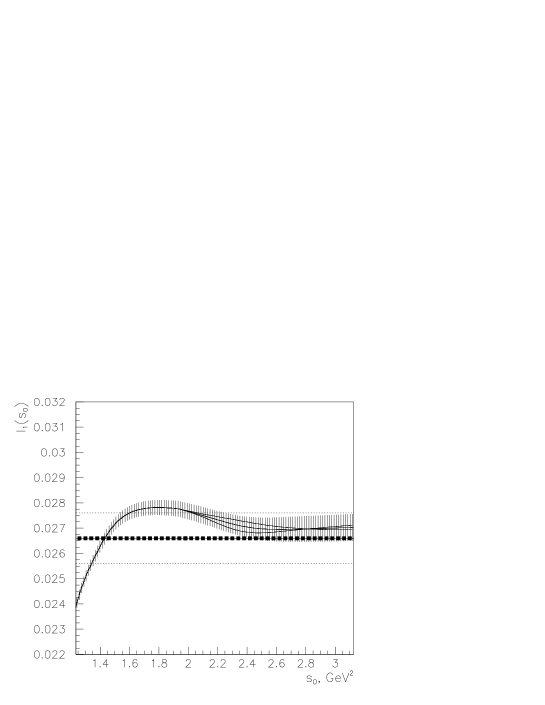
Figure 4: Saturation of the modified DMO sum rule integral (10). The chiral prediction is also shown as in fig.2.

Figure 5: The Laplace-transformed sum rule (12) as a function of the Borel parameter $M^{2}$, compared to the chiral prediction.

Now we use (5) to obtain our third estimate of the spectral integral. The integration results are plotted against the Borel parameter $M^{2}$ in fig.5, assuming standard values for dimension 6 and 8 condensates. The results are independent of $M^{2}$ for $M^{2}>1\,GeV^{2}$, indicating that higher order terms are negligible in this region, and giving

$$I_{2}\equiv I_{2}(\infty)=(27.2\pm 0.4\pm 0.2\pm 0.3)\,10^{-3}\;,$$ (16)

where the last error reflects the sensitivity of (5) to the variation of the condensate values.

One sees that these three numbers (14) – (16) are in good agreement with each other and with the chiral prediction (6). Substitution of our most precise result (15) into (7) yields for the standard value of the pion charge radius quoted above:

$$\alpha_{E}=(2.64\pm 0.36)\,10^{-4}\;{{\rm fm}}^{3},$$ (17)

in good agreement with (3) and the smallest of the measured values, [3]. Note that by substituting a larger value $\langle r_{\pi}^{2}\rangle=0.463\pm 0.006\;{{\rm fm}}^{2}$ [31], one obtains $\alpha_{E}=(3.44\pm 0.30)\,10^{-4}\;{{\rm fm}}^{3}$, about two standard deviations higher than (3).

In conclusion, we have used recent precise data to reconstruct the difference in vector and axial-vector hadronic spectral densities and to study the saturation of Das-Mathur-Okubo and the first Weinberg sum rules. Two methods of improving convergence and decreasing the errors have been used. Within the present level of accuracy, we have found perfect consistence between $\tau$ decay data, chiral and QCD sum rules, the standard value of $\langle r_{\pi}^{2}\rangle$, the average value of $\gamma$ and the chiral prediction for $\alpha_{E}$.

Helpful discussions and correspondence with R. Alemany, R. Barlow, M.Lavelle and P. Poffenberger are gratefully acknowledged.

References

• [1] Y.M.Antipov et al. Z. Phys. C26 (1985) 495.
• [2] T.A.Aibergenov et al. Czech J. Phys. B36 (1986) 948.
• [3] D.Babusci et al. Phys.Lett. B277 (1992) 158.
• [4] M.V.Terent’ev, Sov. J. Nucl. Phys. 16 (1972) 162; B.R.Holstein, Comm. Nucl. Part. Phys. 19 (1990) 221.
• [5] D.A.Bryman et al. Phys. Rep. 88 (1982) 151.
• [6] Particle Data Group Phys. Rev. D50 (1994) 1172. See especially pp. 1447,1448.
• [7] L.E.Piilonen et al., Phys.Rev.Lett. 57 (1986) 1402.
• [8] A.Bay et al. Phys. Lett. B174 (1986) 445.
• [9] V.N.Bolotov et al., Phys.Lett. B243 (1990) 308.
• [10] T.Das, V.Mathur and S.Okubo, Phys. Rev. Lett. 19 (1967) 859; A.I.Vainshtein, JETP Lett. 6 (1967) 815; 7 (1967) 81 (E).
• [11] S.R.Amendolia et al., Phys. Lett. B178 (1986) 244.
• [12] M.O.Lavelle, N.F.Nasrallah and K.Schilcher Phys. Lett. B335 (1994) 211.
• [13] M.Benmerrouche, G.Orlandini and T.G.Steele Phys. Lett. B366 (1996) 354.
• [14] S.Weinberg, Phys. Rev. Lett. 18 (1967) 507.
• [15] V.Kartvelishvili and M.Margvelashvili, Z. Phys. C55 (1992) 83.
• [16] E.Floratos, S.Narison and E.de Rafael, Nucl. Phys. B155 (1979) 115; R.D.Peccei and J.SolΓ , Nucl. Phys. B281 (1987) 1.
• [17] M.Margvelashvili, Phys.Lett. B188 (1988) 763.
• [18] C.A.Dominguez and J.SolΓ , Z. Phys. C40 (1988) 63; V.Kartvelishvili, Phys. Lett. B287 (1992) 159.
• [19] D.Buskulic et al., Z. Phys. C70 (1996) 579.
• [20] S.I.Eidelman and V.N.Ivanchenko, Nucl. Phys. (Proc. Suppl.) B40 (1995) 131.
• [21] D.Bisello et al., Phys. Lett. B220 (1989) 321.
• [22] H.Albrecht et al., Phys.Lett. B185 (1987) 223.
• [23] L.M.Kurdadze et al., JETP Lett. 47 (1988) 512; D.Bisello et al., LAL 91-64, Orsay, 1991.
• [24] M.Artuso et al., Phys.Rev.Lett. 69 (1992) 3278.
• [25] T.E.Coan et al., Phys. Rev. D53 (1996) 6037.
• [26] N.Isgur et al., Phys. Rev. D39 (1989) 1357; J.H.KΓΌhn and A.Santamaria, Z. Phys. C48 (1990) 445.
• [27] R.Akers et al., CERN-PPE/95-022, Geneva, 1995.
• [28] D.Bortoletto et al., Phys.Rev.Lett. 71 (1993) 1791.
• [29] D.Buskulic et al., Phys.Lett. B349 (1987) 585.
• [30] J.J.Gomes-Cadenas et al., Phys.Rev. D42 (1990) 3093; R.Decker et al., Z.Phys. C58 (1993) 445; M.Finkemeier and E.Mirkes, Z.Phys. C69 (1996) 243.
• [31] B.V.Geshkenbein, Z.Phys. C45 (1989) 351.