Compositeness Effects in the Anomalous Weak–Magnetic Moment of Leptons

Abstract

We investigate the effects induced by excited leptons, at the one–loop level, in the anomalous magnetic and weak–magnetic form factors of the leptons. Using a general effective Lagrangian approach to describe the couplings of the excited leptons, we compute their contributions to the weak–magnetic moment of the $\tau$ lepton, which can be measured on the $Z$ peak, and we compare it with the contributions to $g_{\mu}-2$, measured at low energies.

CERN–TH/96–185
July 1996

The standard model of electroweak interactions (SM), in spite of its remarkable agreement with the present experimental data at the $Z$ pole [1], leaves some important questions unanswered. In particular, the reason why fermion generations repeat and the understanding of the complex pattern of quark and lepton masses are not furnished by the model. With the proliferation of fermion flavours, it is natural to ask whether these particles are truly elementary states. The idea of composite models assumes the existence of an underlying structure, characterized by a mass scale $\Lambda$, with the fermions sharing some of the constituents [2]. As a consequence, excited states of each known lepton should show up at some energy scale, and the SM should be seen as the low–energy limit of a more fundamental theory.

We still do not have a satisfactory model, able to reproduce the whole particle spectrum. Due to the lack of a predictive theory, we should rely on a model–independent approach to explore the possible effects of compositeness, employing effective Lagrangian techniques to describe the couplings of these excited states.

Several experimental collaborations have been searching for excited lepton states [3, 4]. Their analyses are based on an effective $SU(2)\times U(1)$ invariant Lagrangian, proposed some years ago by Hagiwara et al. [5]. Also a series of phenomenological studies of excited fermions have been carried out in electron–positron [5, 6, 7, 8, 9, 10], hadronic [8, 9], and electron–proton [5, 10] collisions.

On the other hand, an important source of indirect information about new particles and interactions is the precise measurement of the electroweak parameters. Virtual effects of these new states can alter the SM predictions for some of these parameters, and the comparison with the experimental data can impose bounds on their masses and couplings. Bounds have been derived from the contribution to the anomalous magnetic moment of leptons [11] and to the $Z$ observables at LEP [12].

In this work we use a general effective Lagrangian approach to investigate the effects induced by excited leptons, at the one–loop level, in the anomalous weak–magnetic form factors of the leptons, at an arbitrary energy scale. In particular, we study the contribution to the weak–magnetic moment of the $\tau$ lepton that can be measured on the $Z$ peak [13]. Our results show that for universal couplings the existing limits from $g_{\mu}-2$ strongly constrain the possibility of observing this effect on the anomalous weak–magnetic moment of the $\tau$ lepton at LEP, given the expected experimental sensitivity [13].

We consider excited fermionic states with spin and isospin $\frac{1}{2}$, and we assume that the excited fermions acquire their masses before the $SU(2)\times U(1)$ breaking, so that both left–handed and right–handed states belong to weak isodoublets. The most general dimension–six effective Lagrangian [5, 10] that describes the coupling of the excited–usual fermions, which is $SU(2)\times U(1)$ invariant and CP-conserving, can be written as

$${\cal L}_{Ff}=-\sum_{V=\gamma,Z,W}C_{VFf}\bar{F}\sigma^{\mu\nu}(1-\gamma_{5})f\partial_{\mu}V_{\nu}-i\sum_{V=\gamma,Z}D_{VFf}\bar{F}\sigma^{\mu\nu}(1-\gamma_{5})fW_{\mu}V_{\nu}+\;\text{h.c.}\;,$$ (1)

where $F=N,E$ represent the excited states, and $f=\nu,e$, the usual light fermions of the first generation. A pure left–handed structure is assumed for these couplings in order to comply with the strong bounds coming from the measurement of the anomalous magnetic moment of leptons [11]. The coupling constants $C_{VFf}$ are given by

$$\begin{array}[]{ll}C_{\gamma Ee}=-\frac{\displaystyle e}{\displaystyle 4\Lambda}(f_{2}+f_{1})&\;\;,\;\;\;\;C_{\gamma N\nu}=\frac{\displaystyle e}{\displaystyle 4\Lambda}(f_{2}-f_{1})\\ C_{ZEe}=-\frac{\displaystyle e}{\displaystyle 4\Lambda}(f_{2}\cot\theta_{W}-f_{1}\tan\theta_{W})&\;\;,\;\;\;\;C_{ZN\nu}=\frac{\displaystyle e}{\displaystyle 4\Lambda}(f_{2}\cot\theta_{W}+f_{1}\tan\theta_{W})\\ C_{WE\nu}=C_{WNe}=\frac{\displaystyle e}{\displaystyle 2\sqrt{2}\sin\theta_{W}\Lambda}f_{2}\;,&\end{array}$$ (2)

where $\theta_{W}$ is the weak mixing angle, $f_{2}$ and $f_{1}$ are weight factors associated to the $SU(2)$ and $U(1)$ coupling constants, and $\Lambda$ is the compositeness scale. The quartic interaction coupling constant, $D_{VFf}$, is given by,

$$\begin{array}[]{l}D_{\gamma E\nu}=-D_{\gamma Ne}=-\frac{\displaystyle e^{2}\sqrt{2}}{\displaystyle 4\sin\theta_{W}\Lambda}f_{2}\\ D_{ZE\nu}=-D_{ZNe}=-\frac{\displaystyle e^{2}\sqrt{2}\cos\theta_{W}}{\displaystyle 4\sin^{2}\theta_{W}\Lambda}f_{2}\;.\end{array}$$ (3)

The coupling of gauge bosons to excited leptons can also be described by the $SU(2)\times U(1)$ invariant and CP-conserving effective Lagrangian,

$${\cal L}_{FF}=-\sum_{V=\gamma,Z,W}\bar{F}(A_{VFF}\gamma^{\mu}V_{\mu}+K_{VFF}\sigma^{\mu\nu}\partial_{\mu}V_{\nu})F\;,$$ (4)

where $A_{VFF}$ is given by

$$\begin{array}[]{ll}A_{\gamma EE}=-e&\;\;,\;\;\;\;A_{\gamma NN}=0\\ A_{ZEE}=e\frac{\displaystyle(2\sin^{2}\theta_{W}-1)}{\displaystyle 2\sin\theta_{W}\cos\theta_{W}}&\;\;,\;\;\;\;A_{ZNN}=\frac{\displaystyle e}{\displaystyle 2\sin\theta_{W}\cos\theta_{W}}\\ A_{WEN}=\frac{\displaystyle e}{\displaystyle\sqrt{2}\sin\theta_{W}}&\end{array}$$ (5)

and $K_{VFF}$ is given by

$$\begin{array}[]{ll}K_{\gamma EE}=-\frac{\displaystyle e}{\displaystyle 4\Lambda}(\kappa_{2}+\kappa_{1})&\;\;,\;\;\;\;K_{\gamma NN}=\frac{\displaystyle e}{\displaystyle 4\Lambda}(\kappa_{2}-\kappa_{1})\\ K_{ZEE}=-\frac{\displaystyle e}{\displaystyle 4\Lambda}(\kappa_{2}\cot\theta_{W}-\kappa_{1}\tan\theta_{W})&\;\;,\;\;\;\;K_{ZNN}=\frac{\displaystyle e}{\displaystyle 4\Lambda}(\kappa_{2}\cot\theta_{W}+\kappa_{1}\tan\theta_{W})\\ K_{WEN}=\frac{\displaystyle e}{\displaystyle 2\Lambda}\frac{\displaystyle\kappa_{2}}{\displaystyle\sqrt{2}\sin\theta_{W}}.\end{array}$$ (6)

The matrix element of a boson ($V_{1}$) current has the general form:

$$J^{\mu}=e\;\bar{u}_{f}(p_{1})\;\left\{\frac{1}{2\sin\theta_{W}\cos\theta_{W}}\gamma^{\mu}\left[F_{V}(q^{2})-F_{A}(q^{2})\gamma^{5}\right]+\frac{i}{2m_{f}}a_{f}^{V_{1}}(q^{2})\sigma^{\mu\nu}q_{\nu}\right\}v_{f}(p_{2})$$ (7)

where $V_{1}=\gamma$, or $Z$, and $q=p_{1}+p_{2}$. The terms $F_{V}$ and $F_{A}$ are present at tree level in the SM, e.g. for the $Z$ boson, $F_{V}^{\text{tree}}=-T_{3}^{f}+2Q_{f}\sin^{2}\theta_{W}$, and $F_{A}^{\text{tree}}=-T_{3}^{f}$. The contribution of the excited leptons to these form factors at the one–loop level has been evaluated in Ref. [12]. The anomalous weak–magnetic form factor, $a_{f}^{V_{1}}$, is generated only at one–loop in the SM as well as in the models with excited fermions. In the latter case, there are twelve one–loop Feynman diagrams involving excited fermions that contribute to the anomalous electroweak–magnetic moment of leptons, which are shown in Fig. 1. For each of these contributions, we define the amplitudes $S^{V_{2}}_{i}(q^{2},M^{2},M_{V_{2}}^{2})$, $i=1,\cdots,12$, where $V_{2}$ is the virtual vector boson with mass $M_{V_{2}}$ running in the loops, and we can write the excited lepton contribution to $a_{f}^{V_{1}}$ as

$$a_{f}^{V_{1}}(q^{2})=i\frac{m_{f}^{2}}{e}\;S_{V_{1}\rightarrow\bar{f}f}(q^{2})\;,$$ (8)

with

$$\begin{array}[]{ll}S_{V_{1}\to f^{+}f^{-}}(q^{2})=&S_{1}^{\gamma}(q^{2},M^{2},0)+S_{1}^{Z}(q^{2},M^{2},M_{Z}^{2})+S_{1}^{W}(q^{2},M^{2},M_{W}^{2})\\ &+S_{2+3}^{\gamma}(q^{2},M^{2},0)+S_{2+3}^{Z}(q^{2},M^{2},M_{Z}^{2})+S_{2+3}^{W}(q^{2},M^{2},M_{W}^{2})\\ &+S_{4}^{W}(q^{2},M^{2},M_{W}^{2})\\ &+S_{7+8}^{\gamma}(q^{2},M^{2},0)+S_{7+8}^{Z}(q^{2},M^{2},M_{Z}^{2})+S_{7+8}^{W}(q^{2},M^{2},M_{W}^{2})\\ &+S_{9+10}^{\gamma}(q^{2},M^{2},0)+S_{9+10}^{Z}(q^{2},M^{2},M_{Z}^{2})+S_{9+10}^{W}(q^{2},M^{2},M_{W}^{2})\\ &+S_{11+12}^{W}(q^{2},M^{2},M_{W}^{2})\;.\end{array}$$ (9)

We have neglected the fermion masses in the evaluation of the integrals $S^{V_{2}}_{i}$ (i.e. $m_{f}^{2}\ll M^{2},M_{V}^{2}$), and in this limit $S^{V_{2}}_{5+6}(q^{2},M^{2},M_{V}^{2})=0$.

The loop contributions of the excited leptons were evaluated in $D=4-2\epsilon$ dimensions using the dimension regularization method [14], which is a gauge–invariant regularization procedure, and we adopted the unitary gauge to perform the calculations. The results in $D$ dimensions were obtained with the aid of the Mathematica package FeynCalc [15], and the poles at $D=4$ ($\epsilon=0$) and $D=2$ ($\epsilon=1$) were identified with the logarithmic and quadratic dependence on the scale $\Lambda$ [16].

Our results for $S^{V_{2}}_{i}(q^{2},M^{2},M_{V_{2}}^{2})$ are rather lengthy. We show here only approximate expressions, which are valid in the limit $q^{2},M_{V}^{2}\ll M^{2}$, at first order in $R_{Q}=q^{2}/M^{2}$ and $R_{V}=M_{V}^{2}/M^{2}$:

$$\begin{array}[]{ll}S^{V_{2}}_{1}\simeq&\frac{\displaystyle i}{\displaystyle 144\pi^{2}}\,C^{2}_{V_{2}Ff}\,\Biggl{[}6A_{V_{1}FF}(20+9R_{V})+36K_{V_{1}FF}\,M(3+R_{V})\\ &-R_{Q}(15A_{V_{1}FF}+32K_{V_{1}FF}\,M)-72\left(A_{V_{1}FF}\,+\,K_{V_{1}FF}\,M\right)\log\frac{\displaystyle\Lambda^{2}}{\displaystyle M^{2}}\Biggr{]}\\ S^{V_{2}}_{2+3}\simeq&\frac{\displaystyle i}{\displaystyle 24\pi^{2}}\,C_{V_{2}Ff}C_{V_{1}Ff}\Biggl{\{}g_{V_{2}}^{v}\Bigl{[}3+6R_{V}+12R_{V}\log R_{V}+4R_{Q}\left(1+2\log R_{V}\right)+6\log\frac{\displaystyle\Lambda^{2}}{\displaystyle M^{2}}\Bigr{]}\\ &+g_{V_{2}}^{a}\Bigl{(}39+6R_{V}+12R_{V}\log R_{V}-16R_{Q}\log R_{V}+6\log\frac{\displaystyle\Lambda^{2}}{\displaystyle M^{2}}\Bigr{)}\Biggr{\}}\\ S^{V_{2}}_{4}\simeq&\frac{\displaystyle i}{\displaystyle 144\pi^{2}}\,C^{2}_{V_{2}Ff}g_{V_{1}WW}\Biggl{(}79-9R_{Q}+120R_{V}-42\log\frac{\displaystyle\Lambda^{2}}{\displaystyle M^{2}}\Biggr{)}\\ S^{V_{2}}_{7+8}\simeq&\frac{\displaystyle i}{\displaystyle 2\pi^{2}}\,C_{V_{1}Ff}C_{V_{2}Ff}\left(g_{V_{2}}^{a}+g_{V_{2}}^{v}\right)\Biggl{(}2R_{V}+3R_{V}\log R_{V}-3R_{V}\log\frac{\displaystyle\Lambda^{2}}{\displaystyle M^{2}}+\frac{\displaystyle\Lambda^{2}}{\displaystyle M^{2}}\Biggr{)}\\ S^{V_{2}}_{9+10}\simeq&\frac{\displaystyle i}{\displaystyle 8\pi^{2}}\,C_{V_{1}Ff}C_{V_{2}Ff}\Biggl{\{}A_{V_{1}FF}(15+14R_{V})+K_{V_{1}FF}\,M(22+21R_{V})\\ &-6\Bigl{[}A_{V_{1}FF}(3+2R_{V})+K_{V_{1}FF}\,M(4+3R_{V})\Bigr{]}\log\frac{\displaystyle\Lambda^{2}}{\displaystyle M^{2}}+4\frac{\displaystyle\Lambda^{2}}{\displaystyle M^{2}}\left(A_{V_{2}FF}\,+\,K_{V_{2}FF}\,M\right)\Biggr{\}}\\ S^{V_{2}}_{11+12}\simeq&\frac{\displaystyle i}{\displaystyle 144\pi^{2}}\,C_{V_{2}Ff}\,D_{V_{1}Ff}\,\Biggl{(}1+12R_{V}-6\log\frac{\displaystyle\Lambda^{2}}{\displaystyle M^{2}}\Biggr{)}\end{array}$$ (10)

where $g^{v}_{V_{2}}$ and $g^{a}_{V_{2}}$ are the vector and axial coupling of the vector bosons to the usual fermions: $g^{v}_{\gamma}=-e$, $g^{a}_{\gamma}=0$; $g^{v}_{W}=g^{a}_{W}=g/(2\sqrt{2})$; for $f=\nu$, $g^{v}_{Z}=g^{a}_{Z}=g/(4\cos\theta_{W})$; for $f=e$, $g^{v}_{Z}=g(4\sin^{2}\theta_{W}-1)/(4\cos\theta_{W})$, and $g^{a}_{Z}=-g/(4\cos\theta_{W})$. The coupling $g_{V_{1}WW}$ refers to the triple vector boson vertex: $g_{\gamma WW}=g\sin\theta_{W}$, and $g_{ZWW}=g\cos\theta_{W}$.

We should notice that $S_{2}^{\gamma}$ is infrared–divergent for $q^{2}\neq 0$. However, this divergence cancels against the one coming from real photon emission, and the final result is therefore infrared–finite. In the appendix we present the details of this cancellation.

We give here the approximate final results for the anomalous magnetic ($a_{f}^{\gamma}$) and weak–magnetic ($a_{f}^{Z}$) moments, assuming $M^{2}=\Lambda^{2}\gg M_{W,Z}^{2}$, and $f_{1}=f_{2}=f$ and $k_{1}=k_{2}=k$:

$$\begin{array}[]{l}a_{f}^{\gamma}=\frac{\displaystyle\alpha}{\displaystyle 48\pi}\frac{\displaystyle f^{2}\,m_{f}^{2}}{\displaystyle M^{2}}\left[\frac{\displaystyle 37+74\cos^{2}\theta_{W}+(24+39\cos^{2}\theta_{W})k}{\displaystyle\sin^{2}\theta_{W}\cos^{2}\theta_{W}}\right]\\ a_{f}^{Z}=-\frac{\displaystyle\alpha}{\displaystyle 96\pi}\frac{\displaystyle f^{2}\,m_{f}^{2}}{\displaystyle M^{2}}\left[\frac{\displaystyle 37+2\cos^{2}\theta_{W}(27-74\cos^{2}\theta_{W})+6(4-13\cos^{4}\theta_{W})k}{\displaystyle\sin^{3}\theta_{W}\cos^{3}\theta_{W}}\right]\;.\end{array}$$ (11)

Our results for the anomalous magnetic moment $a_{f}^{\gamma}$ are in agreement with those of Ref. [11], for $k=0$.

We now turn to the attainable values for the weak–magnetic moment of the $\tau$ lepton at LEP energies. In Ref. [13], Bernabeu et al. compute the SM contribution to this observable and discuss the attainable sensitivity at LEP. They claim that it can be measured through the analysis of the angular asymmetry of the semileptonic $\tau$ decay products, which carries information about the weak–magnetic moment of the parent lepton. They assume that the $\tau$ direction is fully reconstructed and they deduce a sensitivity of the order of $|a^{Z}_{\tau}(M_{Z}^{2})|\lesssim 10^{-4}$.

In Fig. 2, we show the accessible region in the parameter space $f$, $k$ and $\Lambda$. For the sake of simplicity we have assumed that $\Lambda=M$. As seen in this figure only models with strong coupling, i.e. $f\simeq\sqrt{4\pi}/e$, and compositeness scale $\Lambda\lesssim 200$ GeV could lead to a value for the anomalous weak–magnetic moment of the $\tau$ large enough to be observed at LEP.

If we assume that the couplings to the excited fermions are universal, i.e. if $f_{i}$, $k_{i}$, $M$ and $\Lambda$ are the same for the three generations, the attainable value for the $\tau$ lepton weak–magnetic moment is already constrained by the existing limits from the anomalous electromagnetic moment of the muon measured at low energies. Nowadays, the most precise determination of the anomalous magnetic moment of the muon $a^{\gamma}_{\mu}\equiv(g_{\mu}-2)/2$ comes from a CERN experiment [17]:

$$a^{\gamma}_{\mu}=11\,659\,230\,(84)\times 10^{-10}.$$ (12)

This result should be compared with the existing theoretical calculations of the QED [18], electroweak [19] and hadronic [20] contributions, which are known with high precision. The main theoretical uncertainty comes from the hadronic contributions which is of the order of $20\times 10^{-10}$. Therefore the present limit on the non–standard contributions to the anomalous magnetic moment of the muon is

$$|\delta\,a^{\gamma}_{\mu}|\lesssim 8\times 10^{-9}\;.$$ (13)

The proposed AGS experiment at the Brookhaven National Laboratory [21] will be able to measure the anomalous magnetic moment of the muon with an accuracy of about $\pm 4\times 10^{-10}$.

In Fig. 3 we show the present limits from Eq. (13) in the parameter space $f$, $k$ and $\Lambda$. Our results for $k=0$ are in agreement with those from Ref. [11]. However, the presence of an anomalous magnetic moment term at tree level in the coupling between a pair of excited fermions (see Eq. (4)) alters the attainable bounds on $f$. As seen in Fig. 3a, there is a value $k=k_{0}\simeq-1.56$ ($-1.72$), for $\Lambda=0.2$ ($1.0$) TeV, for which the limit on the coupling strength $f$ becomes very weak. This comes as a consequence of the cancellation of the leading terms in Eq. (11). The exact dependence of $k_{0}$ on $\Lambda$ is due to higher–order terms, which are not displayed in Eq. (11).

Taking these results into account, we plot in Fig. 4 the attainable values for the $\tau$ anomalous weak–magnetic moment, assuming universal couplings, after imposing the constraints from $g_{\mu}-2$ measurements. We can see that only for a narrow band of $k$ values around $k_{0}$ can $|a^{Z}_{\tau}(M_{Z}^{2})|$ be large enough to be observed at LEP.

Summarizing, we have investigated the effects induced by excited leptons at the one–loop level in the anomalous magnetic and weak–magnetic form factors of the leptons at an arbitrary scale. Using a general effective Lagrangian approach to describe the couplings of the excited leptons, we have computed their contributions to the weak–magnetic moment of the $\tau$, which can be measured on the $Z$ peak, and we compare it with the contributions to $g_{\mu}-2$ measured at low energies. Our results show that although for universal couplings, the existing limits from $g_{\mu}-2$ strongly constrain the possibility of observing the anomalous weak–magnetic moment of the $\tau$ lepton at LEP, there is a very narrow region of parameters in which the observation is still possible. One must notice, however, that in this region the model becomes strongly coupled.

A Cancellation of the Infrared Divergences

The one–loop contribution of excited fermions to the amplitude $Z\rightarrow f\bar{f}$ presents an infrared–divergent piece due to diagrams 2 and 3 of Fig. 1, for $V_{2}=\gamma$. At order $m_{f}^{2}$ the exact expression for the infrared contribution for any $q^{2}$ is

$$M^{\text{IR}}_{2+3} = -\bar{u}(q_{1})\sigma^{\mu\nu}q^{\nu}\epsilon^{\mu}_{V_{1}}(q)v(q_{2})$$

$$\times \left\{\frac{m_{f}}{4\pi^{2}q^{4}}C_{V_{2}Ff}C_{V_{1}Ff}g_{\gamma}^{v}\left[2M^{2}q^{2}+q^{4}+2M^{4}\log\left(1-\frac{q^{2}}{M^{2}}\right)\right]\right\}\;,\log\frac{\lambda^{2}}{M^{2}}$$

where by $\lambda$ we have denoted the photon mass. At order $\alpha^{2}$, this amplitude contributes to the $Z\rightarrow f\bar{f}$ decay width via the interference with the tree–level amplitude

$\displaystyle M_{0}=-i\bar{u}(q_{1})\gamma^{\mu}\epsilon^{\mu}_{V_{1}}(q)(g_{V_{1}}^{v}-g_{V_{1}}^{a}\gamma^{5})v(q_{2})\;,$

yielding

$$\Gamma_{1-\text{loop}}^{\text{IR}}=-\frac{m_{f}^{2}}{24\pi^{3}q^{3}}C_{V_{2}Ff}C_{V_{1}Ff}g_{\gamma}^{v}g_{V_{1}}^{v}\left[2M^{2}q^{2}+q^{4}+2M^{4}\log\left(1-\frac{q^{2}}{M^{2}}\right)\right]\log\frac{\lambda^{2}}{M^{2}}\;.$$ (A1)

This divergence is cancelled against the one coming from the photon bremsstrahlung processes presented in Fig. 5. At order $\alpha^{2}$, the contribution from these diagrams ($M_{a\cdots d}$) to the decay width $Z(q)\to f(q_{1})+\bar{f}(q_{2})+\gamma(k)$ is given by:

$$\Gamma_{\text{bremss}} = \frac{1}{2q(2\pi)^{5}}\int\frac{d^{3}q_{1}}{2E_{1}}\frac{d^{3}q_{2}}{2E_{2}}\frac{d^{3}k}{2k_{0}}\delta^{4}(q-q_{1}-q_{2}-k)\frac{2}{3}\text{Re}\left[(M_{a}+M_{b})^{\dagger}(M_{c}+M_{d})\right]$$

$$= \frac{1}{32q^{3}(2\pi)^{3}}\int_{s_{2\text{min}}}^{s_{2\text{max}}}ds_{2}\int_{s_{1+}}^{s_{1-}}ds_{1}F(s_{1},s_{2})\;,$$

where $s_{2\text{min}}=(m_{f}+\lambda)^{2}$ and $s_{2\text{max}}=(q-m_{f})^{2}$, and

$\displaystyle s_{1\pm}=m_{f}^{2}+\lambda^{2}-\frac{\displaystyle 1}{\displaystyle 2s_{2}}\left[(s_{2}-q^{2}+m_{f}^{2})(s_{2}+\lambda^{2}-m_{f}^{2})\pm f^{1/2}(s_{2},q^{2},m_{f}^{2})f^{1/2}(s_{2},\lambda^{2},m_{f}^{2})\right]$

with the function $f(a,b,c)=(a-b-c)^{2}-4bc$.

At leading order in $m_{f}^{2}$, the infrared–divergent piece of $F(s_{1},s_{2})$ originates from

$\displaystyle F^{\text{IR}}(s_{1},s_{2})=-\frac{32\,m_{f}^{2}}{3}C_{V_{2}Ff}C_{V_{1}Ff}g_{\gamma}^{v}g_{V_{1}}^{v}\Biggl{[}\frac{(s_{1}-m_{f}^{2})^{2}}{(s_{1}-M^{2})(s_{2}-m_{f}^{2})}+\frac{(s_{2}-m_{f}^{2})^{2}}{(s_{2}-M^{2})(s_{1}-m_{f}^{2})}\Biggr{]}\;,$

and we finally get the infrared–divergent contribution from bremsstrahlung as

$\displaystyle\Gamma_{\text{bremss}}^{\text{IR}}=\frac{m_{f}^{2}}{24\pi^{3}q^{3}}C_{V_{2}Ff}C_{V_{1}Ff}g_{\gamma}^{v}g_{V_{1}}^{v}\Biggl{[}2M^{2}q^{2}+q^{4}+2M^{4}\log\left(1-\frac{q^{2}}{M^{2}}\right)\Biggr{]}\log\frac{\lambda^{2}}{M^{2}}=-\Gamma_{1-\text{loop}}^{\text{IR}}$

which exactly cancels the contribution from Eq. (A1).

FIG. 1.: The contribution of the excited leptons to the anomalous electroweak magnetic moments.

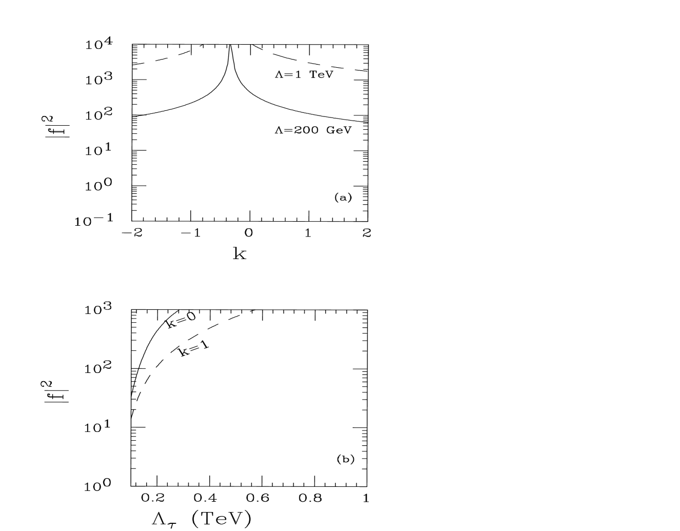
FIG. 2.: (a) Accessible region of parameters for $|a_{\tau}^{Z}(M_{Z}^{2})|\geq 10^{-4}$ (above the curves) in the $|f|^{2}$ versus $k$ plane for fixed values of $M=\Lambda$. (b) Accessible region (above the curves) in the $|f|^{2}$ versus $M=\Lambda$ plane for fixed values of $k$.

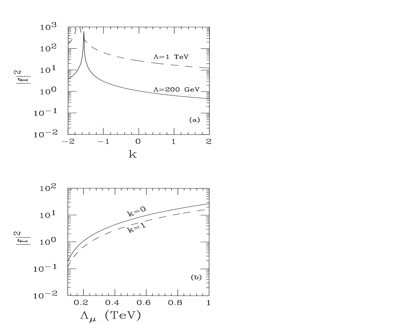
FIG. 3.: (a) Excluded region of parameters from $|a_{\mu}^{\gamma}|\leq 8\times 10^{-9}$ (above the curves) in the $|f|^{2}$ versus $k$ plane for fixed values of $M=\Lambda$. (b) Corresponding limits in the $|f|^{2}$ versus $M=\Lambda$ plane for fixed values of $k$.

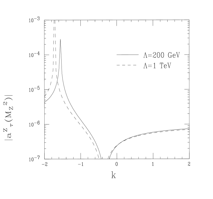
FIG. 4.: Attainable values of $|a_{\tau}^{Z}(M_{Z}^{2})|$ for universal excited lepton couplings after imposing the constraints from $g_{\mu}-2$.

FIG. 5.: Diagrams for photon bremsstrahlung.

REFERENCES

[1] The LEP Collaborations ALEPH, DELPHI, L3,
OPAL, and the LEP Electroweak Working Group, contributions to the
1995 Europhysics Conference on High Energy Physics
(EPS–HEP), Brussels, Belgium, and to the 17th International
Symposium on Lepton–Photon Interactions, Beijing, China,
Report No. CERN–PPE/95–172 (1995).
[2] For a review, see for instance: H. Harari,
Phys. Reports 104 (1984) 159; H. Terazawa, Proceedings
of the XXII International Conference on High Energy Physics,
Leipzig, 1984, edited by A. Meyer and E. Wieczorek, p. 63; W. Buchmüller, Acta Phys. Austriaca, Suppl. XXVII (1985) 517;
M. E. Peskin, Proceedings of the 1985 International Symposium
on Lepton and Photon Interactions at High Energies, Kyoto, 1985, p. 714,
eds. M. Konuma and K. Takahashi.
[3] ALEPH Collaboration, D. Decamp et al.,
Phys. Lett. B236 (1990) 501; id, B250 (1990) 172;
L3 Collaboration, B. Adeva et al., Phys. Lett. B247 (1990) 177; id, B250 (1990) 199 and 205;
id, B252 (1990) 525;
L3 Collaboration, O. Adriani et al., Phys. Lett. B288 (1992) 404;
L3 Collaboration, M. Acciarri et al., Phys. Lett. B353 (1995) 136, id, B370 (1996) 211;
OPAL Collaboration, M. Z. Akrawy et al., Phys. Lett. B240 (1990) 497; id, B241 (1990) 133;
id, B244 (1990) 135; id, B257 (1991) 531;
DELPHI Collaboration, P. Abreu et al., Phys. Lett. B268 (1991) 296; id, B327 (1994) 386;
Z. Phys. C53 (1992) 41.
[4] H1 Collaboration, I. Abt et al., Nucl. Phys. B396 (1993) 3;
ZEUS Collaboration, M. Derrick et al., Phys. Lett. B316 (1993) 207, id, Z. Phys. C65 (1994) 627.
[5] K. Hagiwara, S. Komamiya and D. Zeppenfeld, Z. Phys. C29 (1985) 115.
[6] N. Cabibbo, L. Maiani and Y. Srivastava,
Phys. Lett. B139 (1984) 459;
F. A. Berends and P. H. Daverveldt, Nucl. Phys. B272 (1986)
131;
A. Feldmaier, H. Salecker and F. C. Simm, Phys. Lett. B223 (1989) 234;
M. Martinez, R. Miquel and C. Mana, Z. Phys. C46
(1990) 637;
F. Boudjema and A. Djouadi, Phys. Lett. B240
(1990) 485;
M. Bardadin–Otwinowska, Z. Phys. C55 (1992) 163;
J. C. Montero and V. Pleitez, Phys. Lett. B321
(1994) 267.
[7] I. F. Ginzburg and D. Yu. Ivanov, Phys. Lett. B276 (1992) 214;
T. Kon, I. Ito and Y. Chikashige, Phys. Lett. B287 (1992)
277;
E. Boos, A. Pukhov and A. Beliaev, Phys. Lett. B296
(1992) 452;
O. J. P. Éboli, E. M. Gregores, J. C. Montero, S. F. Novaes and D. Spehler, Phys. Rev. D53 (1996) 1253.
[8] J. Kühn and P. Zerwas, Phys. Lett. B147 (1984) 189.
[9] K. Enqvist and J. Maalampi, Phys. Lett. B135 (1984) 329.
[10] F. Boudjema, A. Djouadi and J. L. Kneur,
Z. Phys. C57 (1993) 425.
[11] S. J. Brodsky and S. D. Drell, Phys. Rev. D22 (1980) 2236; F. M. Renard, Phys. Lett. B116 (1982) 264; P. Merry, S. E. Moubarik, M. Perrottet and
F. M. Renard, Z. Phys. C 46 (1990) 229;
R. Escribano and E. Masso, hep–ph/9607218.
[12] M. C. Gonzalez–Garcia and S. F. Novaes,
CERN–TH/96–123 and IFT–P.013/96.
[13]
J. Bernabeu, G. A. Gonzalez–Sprinberg, M. Tung and J. Vidal,
Nucl. Phys. B436 (1995) 474.
[14] G. ’t Hooft and M. Veltman, Nucl. Phys. B44 (1972) 189; C. G. Bollini and J. J. Giambiagi,
Nuovo Cim. 12B (1972) 20.
[15] R. Mertig, M. Bohm and A. Denner, Comput. Phys. Commun. 64 (1991) 345.
[16] K. Hagiwara, S. Ishihara, R. Szalapski and D. Zeppenfeld, Phys. Lett. B283 (1992) 353; Phys. Rev. D48 (1993) 2182.
[17] J. Bailey et al., Nucl. Phys. B150 (1979) 1;
E. R. Cohen and B. N. Taylor, Rev. Mod. Phys. 59 (1987) 1121.
[18] T. Kinoshita, B. Niz̆ić, and Y. Okamoto, Phys. Rev. Lett. 52 (1984) 717. For a review of
the QED calculations see: T. Kinoshita and W. J. Marciano,
“Quantum Electrodynamics”, T. Kinoshita (ed.), World
Scientific, Singapore (1990), p. 419 and references therein.
[19]
G. Altarelli, N. Cabibbo, and L. Maiani, Phys. Lett. B40 (1972)
415; I. Bars and M. Yoshimura, Phys. Rev. D6 (1972) 374;
K. Fujikawa, B. W. Lee and A. I. Sanda, Phys. Rev. D6 (1972)
2923; R. Jackiw and S. Weinberg, Phys. Rev. D5 (1972) 2473;
W. A. Bardeen, R. Gastmans and B. E. Lautrup, Nucl. Phys. B46
(1972) 319; T. V. Kukhto, E. A. Kuraev, A. Schiller and
Z. K. Silagadze, Nucl. Phys. B371 (1992) 567;
A. Czarnecki, B. Krause and W. J. Marciano, Phys. Rev. D52 (1995)
2619 and Phys. Rev. Lett. 76 (1996) 3267;
S. Peris, M. Perrottet and E. de Rafael, Phys. Lett. B355 (1995) 523.
[20]
J. Calmet, S. Narison, M. Perrottet and E. de Rafael,
Phys. Lett. B61 (1976) 283; Rev. Mod. Phys. 49 (1977) 21;
T. Kinoshita, B. Niz̆ić and Y. Okamoto,
Phys. Rev. D31 (1985) 2108;
E. de Rafael, Phys. Lett. B322 (1994) 239;
E. Pallante, Phys. Lett. B341 (1994) 221;
M. Hayakawa, T. Kinoshita and A. I. Sanda,
Phys. Rev. Lett. 75 (1995) 790;
J. Bijnens, E. Pallante and J. Prades,
Phys. Rev. Lett. 75 (1995) 1447;
S. Eidelman and F. Jegerlehner, Z. Phys. C67 (1995) 585;
K. Adel and F. J. Ynduráin, Univ. Autónoma de Madrid
preprint, FTUAM 95–32 , hep–ph/9509378 (1995).
[21]
B. L. Roberts, Z. Phys. C56 (1992) S101.