QCD SUM RULES AND VIRTUAL COMPTON SCATTERING

In this talk I report on recent progress in a few areas closely related to the virtual Compton scattering studies. In particular, I discuss the quark-hadron duality estimate of the $\gamma^{*}p\to\Delta^{+}$ transition, QCD sum rule calculation of the $\gamma\gamma^{*}\to\pi^{0}$ form factor, and application of perturbative QCD to deeply virtual Compton scattering at small $t$.

1. Soft $vs.$ hard dynamics in QCD

QCD and virtual Compton scattering. The kinematics of the amplitude of the process $\gamma^{*}p\to\gamma p^{\prime}$ can be specified by the initial nucleon momentum $p$, the momentum transfer $r=p-p^{\prime}$ and the momentum $q$ of the initial virtual photon, $q^{2}\equiv-Q^{2}$. The final photon momentum $q^{\prime}$ is then given by $q^{\prime}=q+r$ with $q^{\prime 2}=0$. Other important momentum invariants are $t\equiv(p^{\prime}-p)^{2}=(q-q^{\prime})^{2}$ and $s\equiv(q+p)^{2}$.

Taking $Q^{2}$ large, $i.e.,$ at least above $1\,GeV^{2}$, one can hope to enter the region where the amplitude is dominated by short distances between the two photon vertices and pQCD may be applicable. In this situation, it is tempting to speak about the “virtual Compton scattering on a single quark” implying that the large-$Q^{2}$ behaviour is given just by the quark propagator (see Fig.$1a$), while the long-distance information is accumulated in a distribution function $F(X,t)$ described by the matrix element of $\langle p^{\prime}|\bar{q}\ldots q|p\rangle$ type. However, the factorization formula

$$M(Q^{2},s,t)\to\int m(s/Q^{2},X)F(X,t)dX$$ (1)

only makes sense if $|t|\ll Q^{2}$. Otherwise, if $|t|\sim Q^{2}$, large momentum enters into the hadron wave function and one deals with the scattering process on the hadron as a whole.

                 

Figure 1: $a)$ Handbag diagram contributing to the DVCS amplitude at $t=0$. The lower blob corresponds to the double quark distribution $F(x,y)$. $b)$ One of the two-gluon-exchange diagrams dominating the VCS amplitude for asymptotically large $Q^{2}$ and $t$. $c)$ Lowest-order diagram for the $\gamma^{*}\gamma\to\pi^{0}$ transition form factor. The blob corresponds to the pion distribution amplitude $\varphi_{\pi}(x)$.

For $|t|\ll Q^{2}$, the function $F(X,t)$ in eq.(1) looks like a parton distribution function $f(x)$ with an additional form-factor-type dependence on $t$. To make analogy with deep inelastic scattering, it is instructive to recall that the imaginary part of the virtual forward Compton amplitude (for which $q^{\prime}=q$ and $p^{\prime}=p$) in the limit of large $Q^{2}$ and fixed Bjorken variable $\zeta\equiv Q^{2}/2(pq)$ can be written as

$$\int_{0}^{1}f(x)\delta((q+xp)^{2})\cdot 2(qp)dx=\int_{0}^{1}f(x)\delta(x-Q^{2}/2(qp))dx=f(\zeta)\,,$$ (2)

where $xp$ is the fraction of the initial hadron momentum carried by the interacting quark. The usual parton distribution functions $f(\zeta)$ correspond to exactly forward matrix elements, with $r\equiv p^{\prime}-p=0$, while the kinematics of VCS requires that $r\neq 0$ and $t\equiv r^{2}\neq 0$. Hence, we need a new type of parton functions $F(X,t)$ $\!{}^{{\bf?}}$. In the limit $t\to 0$, they reduce to the “asymmetric distribution functions” $F(X)$ $\!{}^{{\bf?},{\bf?}}$. Hence, the studies of deeply virtual Compton scattering (DVCS) are related to a new field of pQCD applications. As shown in refs.$\!{}^{{\bf?},{\bf?}}$, the asymmetric distributions $F(X)$ have features of both the distribution functions and distribution amplitudes (wave functions). A more detailed discussion of DVCS at small $t$ will be given in Section 3.

Another situation in which pQCD is applicable is when both $Q^{2}$ and $|t|$ are asymptotically large. Then the virtual Compton scattering amplitude factorizes into a convolution of the short-distance amplitude $m(\{x_{i}\},\{y_{j}\},Q^{2},s,t)$ and two distribution amplitudes $\varphi(x_{1},x_{2},x_{3})$, $\varphi(y_{1},y_{2},y_{3})$ describing the proton in the initial and final state, respectively (see Fig.$1b$). They are related to matrix elements of $\langle 0|q\ldots q\ldots q|p\rangle$ type and give the probability amplitude, that $e.g.,$ the initial proton can be treated as three collinear quarks with the momentum $p$ divided into fractions $x_{1}p,x_{2}p,x_{3}p$ with $x_{1}+x_{2}+x_{3}=1$. The short-distance amplitude $m(\{x_{i}\},\{y_{j}\},Q^{2},s,t)$ is given by Feynman diagrams involving two hard gluon exchanges, suppressed by a factor $(\alpha_{s}/\pi)^{2}\sim 1/100$ compared to the “soft contribution” produced by a simple overlap of soft wave functions, without any gluon exchanges. The soft term, however, has an extra power of $1/Q^{2}$ for large $Q^{2}$. As a result, the hard term asymptotically dominates, though the soft term may be much larger than the hard one for accessible $Q^{2}$.

Quark-hadron duality and $\gamma^{*}p\to\Delta^{+}$ transition. In particular, a purely soft contribution to $G_{M}^{p}(Q^{2})$ calculated within the local quark-hadron duality approach $\!{}^{{\bf?}}$ is in good agreement with experimental data up to $Q^{2}\sim\,20\,GeV^{2}$. The same approach was used recently $\!{}^{{\bf?}}$ to get the estimates of the soft term for the $\gamma^{*}p\to\Delta^{+}$ transition. For the magnetic form factor $G_{M}^{*}(Q^{2})$ these estimates are rather close to the results of the analysis of inclusive SLAC data $\!{}^{{\bf?},{\bf?}}$. A small value for the ratio $G_{E}^{*}(Q^{2})/G_{M}^{*}(Q^{2})$ obtained in ref.$\!{}^{{\bf?}}$ is also in agreement with available data $\!{}^{{\bf?}}$, in contrast to the pQCD prediction $\!{}^{{\bf?}}$ which gives $G_{E}^{*}(Q^{2})/G_{M}^{*}(Q^{2})\to\,-1$ for the ratio of hard contributions.

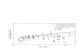
Figure 2: Quark-hadron duality estimates for the $\gamma^{*}p\to\Delta^{+}$ transition. Left: form factor $G_{M}^{*}(Q^{2})$. Right: ratio of form factors $G_{E}^{*}(Q^{2})$ and $G_{M}^{*}(Q^{2})$.

Within different nonperturbative approaches $\!{}^{{\bf?},{\bf?},{\bf?},{\bf?}}$, it was observed that soft terms are sufficiently large to describe the data or that the hard terms are too small compared to the data. Hence, there is a growing evidence that soft terms dominate the exclusive amplitudes at accessible energies. Of course, the magnitude of the hard contribution depends on the shape of distribution amplitudes (DA’s). The latter are usually integrated with the weights like $1/x_{1}x_{2}$, so the humpy DA’s of Chernyak-Zhitnitsky (CZ) type $\!{}^{{\bf?},{\bf?}}$ produce contributions which are much larger than those obtained with smooth DA’s close to the “asymptotic” forms. The CZ wave functions were originally motivated by QCD sum rule analysis $\!{}^{{\bf?}}$. However, the results of the QCD sum rule calculations of the DA’s are extremely model-dependent and unreliable. Furthermore, for the theoretically most clean case of the $\gamma^{*}\gamma\to\pi^{0}$ form factor, both a direct QCD sum rule calculation of this form factor and available experimental data show no enhancement compared to the pQCD result obtained with the asymptotic DA for the pion.

2. $\gamma^{*}\gamma\to\pi^{0}$ form factor

pQCD analysis. The transition $\gamma^{*}\gamma^{*}\to\pi^{0}$ of two virtual photons $\gamma^{*}$ into a neutral pion provides an exceptional opportunity to test QCD predictions for exclusive processes. In the lowest order of perturbative QCD, its asymptotic behaviour is due to the subprocess $\gamma^{*}(q)+\gamma^{*}(q^{\prime})\to\bar{q}(\bar{x}p)+q(xp)$ with $x$ ($\bar{x}$) being the fraction of the pion momentum $p$ carried by the quark produced at the $q$ ($q^{\prime})$ photon vertex (see Fig.1$c$). The relevant diagram is similar to the handbag diagram for deep inelastic scattering, with the main difference that one should use the pion distribution amplitude $\varphi_{\pi}(x)$ instead of parton densities. For large $Q^{2}$, the perturbative QCD prediction is given by $\!{}^{{\bf?}}$:

$$F_{\gamma^{*}\gamma^{*}\pi^{0}}^{as}(Q^{2},q^{\prime 2})=\frac{4\pi}{3}\int_{0}^{1}{{\varphi_{\pi}(x)}\over{xQ^{2}-\bar{x}q^{\prime 2}}}\,dx\stackrel{{\scriptstyle q^{\prime 2}=0}}{{\longrightarrow}}\frac{4\pi}{3}\int_{0}^{1}{{\varphi_{\pi}(x)}\over{xQ^{2}}}\,dx\equiv\frac{4\pi}{3Q^{2}}I\,.$$ (3)

Experimentally, the most important situation is when the lower virtuality photon is (almost) real $q^{\prime 2}\approx 0$. In this case, necessary nonperturbative information is accumulated in the same integral $I$ (see eq.(3)) that appears in the one-gluon-exchange diagram for the pion electromagnetic form factor $\!{}^{{\bf?},{\bf?},{\bf?}}$. The value of $I$ depends on the shape of the pion distribution amplitude $\varphi_{\pi}(x)$. In particular, using the asymptotic form $\varphi_{\pi}^{as}(x)=6f_{\pi}x\bar{x}$ $\!{}^{{\bf?},{\bf?}}$ gives $F_{\gamma\gamma^{*}\pi^{0}}^{as}(Q^{2})=4\pi f_{\pi}/Q^{2}$ for the asymptotic behaviour $\!{}^{{\bf?}}$. If one takes the Chernyak-Zhitnitsky form $\!{}^{{\bf?}}$ $\varphi_{\pi}^{CZ}(x)=30f_{\pi}x(1-x)(1-2x)^{2}$, the integral $I$ increases by a sizable factor of 5/3, and this difference can be used for experimental discrimination between the two forms.

Note, that the pQCD hard scattering term for $\gamma\gamma^{*}\to\pi^{0}$ has the zeroth order in the QCD coupling constant $\alpha_{s}$, just like in deep inelastic scattering. Hence, there are good reasons to expect that pQCD for $F_{\gamma\gamma^{*}\pi^{0}}(Q^{2})$ may work at rather low $Q^{2}$. The $Q^{2}=0$ limit of $F_{\gamma\gamma^{*}\pi^{0}}(Q^{2})$ is known from $\pi^{0}\to\gamma\gamma$ decay rate. Using PCAC and ABJ anomaly $\!{}^{{\bf?}}$, one can calculate $F_{\gamma\gamma^{*}\pi^{0}}(0)$ theoretically: $F_{\gamma\gamma^{*}\pi^{0}}(0)=1/\pi f_{\pi}.$ It is natural to expect that a complete QCD result does not strongly deviate from a simple interpolation $\!{}^{{\bf?}}$ $\pi f_{\pi}F_{\gamma\gamma^{*}\pi^{0}}(Q^{2})=1/(1+Q^{2}/4\pi^{2}f_{\pi}^{2})$ between the $Q^{2}=0$ value and the large-$Q^{2}$ asymptotics . This interpolation implies the asymptotic form of the distribution amplitude for the large-$Q^{2}$ limit and agrees with CELLO experimental data $\!{}^{{\bf?}}$. It was also claimed $\!{}^{{\bf?}}$ that the new CLEO data available up to $8\,GeV^{2}$ also agree with the interpolation formula.

Comparing the data with theoretical predictions, one should take into account the one-loop pQCD radiative corrections to the hard scattering amplitude calculated in ref.$\!{}^{{\bf?}}$. Effectively, the correction decreases the leading-order result by about $20\%$, still leaving a sizable gap between the prediction based on the CZ amplitude and the phenomenologically successful Brodsky-Lepage interpolation formula$\!{}^{{\bf?}}$. Hence, the new preliminary data$\!{}^{{\bf?}}$ seem to indicate that the magnitude of $I$ is close to that corresponding to the asymptotic form of the pion distribution amplitude. Because of the far-reaching consequences of this conclusion, it is desirable to have a direct calculation of the $\gamma\gamma^{*}\to\pi^{0}$ form factor in the intermediate region of moderately large momentum transfers $Q^{2}\raisebox{-0.86108pt}{$\stackrel{{\scriptstyle\textstyle>}}{{\raisebox{-2.58334pt}[0.0pt][0.0pt]{$\sim$}}}$}1\,GeV^{2}$. As we will see below, the QCD sum rules allow one to calculate $F_{\gamma\gamma^{*}\pi^{0}}(Q^{2})$ for large $Q^{2}$ without any assumptions about the shape of the pion distribution amplitude, and the result can be used to get information about $\varphi_{\pi}(x)$.

QCD sum rules and pion distribution amplitude. The CZ sum rule written directly for the pion distribution amplitude $\varphi_{\pi}(x)$ is

$$f_{\pi}\varphi_{\pi}(x) = \frac{3M^{2}}{2\pi^{2}}(1-e^{-s_{0}/M^{2}})x(1-x)+\frac{\alpha_{s}\langle GG\rangle}{24\pi M^{2}}[\delta(x)+\delta(1-x)]$$ (4)

$$+ \frac{8}{81}\frac{\pi\alpha_{s}\langle\bar{q}q\rangle^{2}}{M^{4}}\{11[\delta(x)+\delta(1-x)]+2[\delta^{\prime}(x)+\delta^{\prime}(1-x)]\}.$$

Here, $M$ is the auxiliary Borel parameter which must be taken in the region where the r.h.s. is least sensitive to its variations, and $s_{0}$ is the effective onset of the continuum fitted to maximize the $M^{2}$-stability region. From the QCD sum rule for $f_{\pi}$, $\!{}^{{\bf?}}$ $s_{0}\approx 0.7\,GeV^{2}$. As emphasized in ref.$\!{}^{{\bf?}}$, the lowest condensates $\langle GG\rangle$ and $\langle\bar{q}q\rangle^{2}$ taken into account in eq.(4) do not provide all the information necessary for a reliable determination of $\varphi_{\pi}(x)$. The humpy CZ shape is, in fact, a compromise between the $\delta(x)$, $\delta(1-x)$ condensate peaks and the smooth $x(1-x)$ behaviour of the perturbative term. Adding higher condensates, $e.g.,$ $\langle\bar{q}D^{2}q\rangle$, one would get even higher derivatives of $\delta(x)$ and $\delta(1-x)$. The sum of such singular terms can be treated as an expansion of some finite-width function $\delta\varphi(x)$:

$$\delta\varphi(x)=a_{0}\delta(x)+a_{1}\delta^{\prime}(x)+a_{2}\delta^{\prime\prime}(x)+\ldots+\{x\to 1-x\}.$$ (5)

Of course, the knowledge of $a_{0}$ alone is not sufficient for a reliable reconstruction of $\delta\varphi(x)$. On the other hand, the higher coefficients $a_{1},a_{2},etc.$ are given by a sum of several higher condensates whose magnitudes are completely unknown. Hence, no strict conclusions can be made. The CZ procedure is equivalent to assuming that $a_{1},a_{2},\ldots\,\sim 0$, though other choices ($e.g.,$ nonlocal condensate model $\!{}^{{\bf?}}$) may look more realistic.

QCD sum rule for doubly virtual form factor $F_{\gamma^{*}\gamma^{*}\pi^{0}}(q^{2},q^{\prime 2})$. Instead of following the steps dictated by the old logic: $1)$ pQCD factorization for $F_{\gamma^{*}\gamma\pi^{0}}(Q^{2})$; $2)$ QCD sum rules for the moments of $\varphi_{\pi}(x)$ (which are unreliable); $3)$ calculation of $I=\int_{0}^{1}\varphi_{\pi}(x)/x\,dx$, we developed in ref. $\!{}^{{\bf?}}$ the approach which $1)$ starts with the QCD sum rule for $F_{\gamma^{*}\gamma^{*}\pi^{0}}(q^{2},q^{\prime 2})$ in the $q^{\prime 2}\to 0$ limit; $2)$ information about $I$ is extracted from this sum rule and $3)$ then used to make conclusions about the shape of $\varphi_{\pi}(x)$. When both virtualities of the photons are large, we have the following QCD sum rule:

$$\pi f_{\pi}\mbox{$F_{\gamma^{*}\gamma^{*}\pi^{\circ}}$}(Q^{2},q^{\prime 2})=2\int_{0}^{s_{o}}ds\,e^{-s/{M^{2}}}\int_{0}^{1}\frac{x\bar{x}(xQ^{2}-\bar{x}q^{\prime 2})^{2}}{[s{x}\bar{x}+xQ^{2}-\bar{x}q^{\prime 2}]^{3}}\,dx\,$$

$$+\frac{\pi^{2}}{9}{\langle\frac{\alpha_{s}}{\pi}GG\rangle}\left(\frac{1}{2M^{2}Q^{2}}-\frac{1}{2M^{2}q^{\prime 2}}+\frac{1}{Q^{2}q^{\prime 2}}\right)$$

$$+\frac{64}{243}\pi^{3}\alpha_{s}{\langle\bar{q}q\rangle}^{2}\left(\frac{1}{M^{4}}\left[\frac{Q^{2}}{q^{\prime 4}}-\frac{9}{2q^{\prime 2}}+\frac{9}{2Q^{2}}-\frac{q^{\prime 2}}{Q^{4}}\right]+\frac{9}{Q^{2}q^{\prime 4}}-\frac{9}{Q^{4}q^{\prime 2}}\right).$$ (6)

In this situation, the pQCD approach is also expected to work. Indeed, neglecting the $s{x}\bar{x}$-term compared to $xQ^{2}-\bar{x}q^{\prime 2}$ and keeping only the leading $O(1/Q^{2})$ and $O(1/q^{\prime 2})$ terms in the condensates, we can write eq.(6) as

$$\mbox{$F_{\gamma^{*}\gamma^{*}\pi^{\circ}}$}(,Q^{2})=\frac{4\pi}{3f_{\pi}}\int_{0}^{1}\frac{dx}{xQ^{2}-\bar{x}q^{\prime 2}}\,\left\{\frac{3M^{2}}{2\pi^{2}}(1-e^{-s_{0}/M^{2}})x\bar{x}\right.$$

$$\left.+\frac{1}{24M^{2}}\langle\frac{\alpha_{s}}{\pi}GG\rangle[\delta(x)+\delta(\bar{x})]\right.$$

$$+\left.\frac{8}{81M^{4}}\pi\alpha_{s}{\langle\bar{q}q\rangle}^{2}\biggl{(}11[\delta(x)+\delta(\bar{x})]+2[\delta^{\prime}(x)+\delta^{\prime}(\bar{x})]\biggr{)}\right\}.$$ (7)

The expression in curly brackets coincides with the QCD sum rule (4) for the pion distribution amplitude $f_{\pi}\varphi_{\pi}(x)$. Hence, when both $Q^{2}$ and $q^{\prime 2}$ are large, the QCD sum rule (6) exactly reproduces the pQCD result (3).

One may be tempted to get a QCD sum rule for the integral $I$ by taking $q^{\prime 2}=0$ in eq.(6). Such an attempt, however, fails immediately because of the power singularities $1/q^{\prime 2}$, $1/q^{\prime 4}$, $etc.$ in the condensate terms. It is easy to see that these singularities are produced by the $\delta(x)$ and $\delta^{\prime}(x)$ terms in eq.(7). In fact, it is precisely these terms that generate the two-hump form for $\varphi_{\pi}(x)$ in the CZ-approach $\!{}^{{\bf?}}$. The advantage of having a direct sum rule for $F_{\gamma\gamma^{*}\pi^{0}}(Q^{2},q^{\prime 2})$ is that the small-$q^{\prime 2}$ behavior of $F_{\gamma\gamma^{*}\pi^{0}}(Q^{2},q^{\prime 2})$ is determined by the position of the closest resonances in the $q^{\prime}$ channel, which is known. Eventually, $1/q^{\prime 2}$ is substituted for small $q^{\prime 2}$ by something like $1/m_{\rho}^{2}$ and the QCD sum rule in the $q^{\prime 2}$ limit is

$$\pi f_{\pi}F_{\gamma\gamma^{*}\pi^{0}}(Q^{2})=\int_{0}^{s_{0}}\left\{1-2\frac{Q^{2}-2s}{(s+Q^{2})^{2}}\left(s_{\rho}-\frac{s_{\rho}^{2}}{2m_{\rho}^{2}}\right)\right.$$

$$+ \left.2\frac{Q^{2}-6s+3s^{2}/Q^{2}}{(s+Q^{2})^{4}}\left(\frac{s_{\rho}^{2}}{2}-\frac{s_{\rho}^{3}}{3m_{\rho}^{2}}\right)\right\}e^{-s/M^{2}}\frac{Q^{2}ds}{(s+Q^{2})^{2}}$$

$$+ \frac{\pi^{2}}{9}{\langle\frac{\alpha_{s}}{\pi}GG\rangle}\left\{\frac{1}{2Q^{2}M^{2}}+\frac{1}{Q^{4}}-2\int_{0}^{s_{0}}e^{-s/M^{2}}\frac{ds}{(s+Q^{2})^{3}}\right\}$$

$$+ \frac{64}{27}\pi^{3}\alpha_{s}{\langle\bar{q}q\rangle}^{2}\lim_{\lambda^{2}\to 0}\left\{\frac{1}{2Q^{2}M^{4}}+\frac{12}{Q^{4}m_{\rho}^{2}}\left[\log\frac{Q^{2}}{\lambda^{2}}-2\right.\right.$$

$$+ \left.\left.\int_{0}^{s_{0}}e^{-s/M^{2}}\left(\frac{s^{2}+3sQ^{2}+4Q^{4}}{(s+Q^{2})^{3}}-\frac{1}{s+\lambda^{2}}\right)ds\right]\right.$$

$$- \left.\frac{4}{Q^{6}}\left[\log\frac{Q^{2}}{\lambda^{2}}-3+\int_{0}^{s_{0}}e^{-s/M^{2}}\left(\frac{s^{2}+3sQ^{2}+6Q^{4}}{(s+Q^{2})^{3}}-\frac{1}{s+\lambda^{2}}\right)ds\right]\right\}.$$

In Fig.3, we present a curve for $Q^{2}F_{\gamma\gamma^{*}\pi^{0}}(Q^{2})/4\pi f_{\pi}$ calculated from eq.(2.) for standard values of the condensates, $\rho$- and $\pi$-meson duality intervals $s_{\rho}=1.5\,GeV^{2}$, $\!{}^{{\bf?}}$, $s_{0}=0.7\,GeV^{2}$ and $M^{2}=0.8\,GeV^{2}$. It is rather close to the curve corresponding to the Brodsky-Lepage interpolation formula $\pi f_{\pi}F_{\gamma\gamma^{*}\pi^{0}}(Q^{2})=1/(1+Q^{2}/4\pi^{2}f_{\pi}^{2})$ and to that based on the $\rho$-pole approximation $\pi f_{\pi}F(Q^{2})=1/(1+Q^{2}/m_{\rho}^{2})$. Hence, our result favors a pion distribution amplitude which is close to the asymptotic form. It should be noted, that the $\rho$-pole behaviour in the $Q^{2}$-channel has nothing to do with the explicit use of the $\rho$-contributions in our models for the correlators in the $q^{\prime 2}$-channel: the $Q^{2}$-dependence of the $\rho$-pole type emerges due to the fact that the pion duality interval $s_{0}\approx 0.7\,GeV^{2}$ is numerically close to $m_{\rho}^{2}\approx 0.6\,GeV^{2}$. Taking the lowest-order perturbative spectral density $\rho^{quark}(s,q^{\prime 2}=0,Q^{2})={{Q^{2}}/{(s+Q^{2})^{2}}}$ and assuming the local quark-hadron duality, we obtain the result

$$f_{\pi}F_{\gamma\gamma^{*}\pi^{0}}^{LD}(Q^{2})=\frac{1}{\pi}\int_{0}^{s_{0}}\rho^{quark}(s,0,Q^{2})\,ds=\frac{1}{\pi(1+Q^{2}/s_{0})}$$ (9)

coinciding, for $s_{0}=4\pi^{2}f_{\pi}^{2}\approx 0.67\,GeV^{2}$ with the BL-interpolation formula.

             

Figure 3: Combination $Q^{2}F_{\gamma\gamma^{*}\pi^{0}}(Q^{2})/4\pi f_{\pi}$ as calculated from the QCD sum rule (solid line), $\rho$-pole model (short-dashed line) and Brodsky-Lepage interpolation (long-dashed line).

Lessons. $1)$ CZ sum rule is an unreliable source of information about the pion DA; $2)$ Pion DA is narrow; $3)$ Since the diagrams for the nucleon DA’s have the structure as in the pion case, we should expect that the nucleon DA’s are also close to asymptotic and , hence, the two-gluon-exchange hard terms are very small for accessible $Q^{2}$ and $t$. Thus, it is very important to get the estimates for the soft contributions to the virtual Compton scattering amplitude (see, $e.g.,$ refs. $\!{}^{{\bf?}}$, where the high-$t$ real Compton scattering on the pion was considered).

3. Small-$t$, large-$Q^{2}$ limit of VCS: a new pQCD area

Recently, X. Ji $\!{}^{{\bf?}}$ suggested to use the deeply virtual Compton scattering (DVCS) to get information about some parton distribution functions inaccessible in standard inclusive measurements. He also emphasized that the DVCS amplitude has a scaling behavior in the region of small $t$ and fixed $x_{Bj}$ which makes it a very interesting object on its own ground.

Double distributions. In the scaling limit, the square of the proton mass $m_{p}^{2}=p^{2}$ can be neglected compared to the virtuality $Q^{2}\equiv-q^{2}$ of the initial photon and the energy invariant $p\cdot q\equiv m_{p}\nu$. Thus, we set $p^{2}=0$ and, for small $t$, we also have $r^{2}=0$. Then the requirement $p^{\prime 2}\equiv(p-r)^{2}=p^{2}$ reduces to the condition $p\cdot r=0$ which can be satisfied only if $r$ is proportional to $p$: $r=\zeta p$, where $\zeta$ coincides with the Bjorken variable $x_{Bj}\equiv Q^{2}/2(p\cdot q)$, $0\leq x_{Bj}\leq 1$. Naturally, the light-like limit of 4-momenta $p$, $r$ is more convenient to visualize in a frame where the initial proton is moving fast, rather than in its rest frame.

Though the momenta $p$ and $r$ are proportional to each other, one should make a clear distinction between them since $p$ and $r$ specify the momentum flow in two different channels. Since the initial quark momentum originates both from $p$ and $r$, we write it as $xp+yr$. In more formal terms, the relevant light-cone matrix elements are parameterized as

$$\langle p-r\,|\,\bar{\psi}_{a}(0)\hat{z}E(0,z;A)\psi_{a}(z)\,|\,p\rangle|_{z^{2}=0}=\bar{u}(p-r)\hat{z}u(p)$$ (10)

$$\int_{0}^{1}\int_{0}^{1}\,\left(e^{-ix(pz)-iy(rz)}F_{a}(x,y)\right.-\left.e^{ix(pz)-i\bar{y}(rz)}F_{\bar{a}}(x,y)\right)\,\theta(x+y\leq 1)dy\,dx,$$

$etc.,$ where $\hat{z}\equiv\gamma_{\mu}z^{\mu}$ and $\bar{u}(p-r),u(p)$ are the Dirac spinors for the nucleon.

Taking the limit $r=0$ gives the matrix element defining the parton distribution functions $f_{a}(x)$, $f_{\bar{a}}(x)$. This leads to the reduction formula:

$$\int_{0}^{1-x}\,F_{a}(x,y)\,dy=f_{a}(x).$$ (11)

Asymmetric distribution functions. Since $r=\zeta p$, the variable $y$ appears in eq.(10) only in $x+y\zeta\equiv X$ and $x-\bar{y}\zeta\equiv X-\zeta$ combinations, where $X$ and $(X-\zeta)$ are the total fractions of the initial hadron momentum $p$ carried by the quarks. Integrating the double distribution $F(X-y\zeta,y)$ over $y$ we get the asymmetric distribution function

$${\cal F}_{\zeta}^{a}(X)=\int_{0}^{{\rm min}\{X/\zeta,\bar{X}/\bar{\zeta}\}}F_{a}(X-y\zeta,y)\,dy,$$ (12)

where $\bar{\zeta}\equiv 1-\zeta$. Since $\zeta\leq 1$ and $x+y\leq 1$, the variable $X$ satisfies a natural constraint $0\leq X\leq 1$. In the region $X>\zeta$ (Fig.4$a$), the initial quark momentum $Xp$ is larger than the momentum transfer $r=\zeta p$, and we can treat ${\cal F}_{\zeta}^{a}(X)$ as a generalization of the usual distribution function $f_{a}(x)$. In this case, the quark goes out of the hadron with a positive fraction $Xp$ of the original hadron momentum and then comes back into the hadron with a changed (but still positive) fraction $(X-\zeta)p$. The Bjorken ratio $\zeta$ specifies the momentum asymmetry of the matrix element. Hence, one deals now with a family of asymmetric distribution functions ${\cal F}_{\zeta}^{a}(X)$ whose shape changes when $\zeta$ is changed. The basic distinction between the double distributions $F(x,y)$ and the asymmetric distribution functions ${\cal F}_{\zeta}(X)$ is that the former do not depend on the momentum asymmetry parameter $\zeta$, while the latter are explicitly labelled by it.

                  

Figure 4: Momentum flow corresponding to the asymmetric distribution function in two regimes: a) $X\geq\zeta$ and b) $X\equiv Y\zeta\leq\zeta$.

When $\zeta\to 0$, the limiting curve for ${\cal F}_{\zeta}(X)$ reproduces the usual distribution function:

$${\cal F}^{a}_{\zeta=0}\,(X)=f_{a}(X)\ .$$ (13)

Another region is $X<\zeta$ (Fig.4$b$), in which the “returning” quark has a negative fraction $(X-\zeta)$ of the light-cone momentum $p$. Hence, it is more appropriate to treat it as an antiquark going out of the hadron and propagating together with the original quark. Writing $X$ as $X=Y\zeta$, we see that the quarks carry now positive fractions $Y\zeta p\equiv Yr$ and $\bar{Y}r\equiv(1-Y)r$ of the momentum transfer $r$, and the asymmetric distribution function in the region $X=Y\zeta<\zeta$ looks like a distribution amplitude $\Psi_{\zeta}(Y)$ for a $\bar{q}q$ state with the total momentum $r=\zeta p$:

$$\Psi_{\zeta}(Y)=\int_{0}^{Y}F((Y-y)\zeta,y)\,dy.$$ (14)

Leading-order contribution. Using the parameterization for the matrix elements given above, we get a parton-type representation for the handbag contribution at $t=0$:

$$T^{\mu\nu}_{symm}(p,q,r)=\left(g^{\mu\nu}-\frac{1}{p\cdot q}(p^{\mu}q^{\nu}+p^{\nu}q^{\mu})\right)\,\sum_{a}e_{a}^{2}\,\sqrt{1-\zeta}\ (T_{V}^{a}(\zeta)+T_{V}^{\bar{a}}(\zeta)),$$

where only the $\{\mu\leftrightarrow\nu\}$-symmetric part is shown explicitly and $T_{V}^{a}(\zeta)$ is the invariant amplitude depending on the scaling variable $\zeta$:

$$T_{V}^{a}(\zeta)=\int_{0}^{1}\left(\frac{1}{X-\zeta+i\epsilon}+\frac{1}{X}\right){\cal F}_{\zeta}^{a}(X)\,dX\,.$$ (15)

The term containing $1/(X-\zeta+i\epsilon)$ generates the imaginary part:

$$-\frac{1}{\pi}\,{\rm Im}\,T_{V}^{a}(\zeta)={\cal F}^{a}_{\zeta}\,(\zeta)\,.$$ (16)

Though ${\cal F}_{\zeta=0}^{a}(X)=f_{a}(X)$, in the general case when $\zeta\neq 0$, these two functions differ. Furthermore, the imaginary part appears for $X=\zeta$, $i.e.,$ in a highly asymmetric configuration in which the second quark carries a vanishing fraction of the original hadron momentum, in contrast to the usual distribution $f_{a}(\zeta)$ which corresponds to a symmetric configuration with the final quark having the momentum equal to that of the initial one. A characteristic feature of the asymmetric distribution functions ${\cal F}_{\zeta}^{a}(X)$ is that they rapidly vary in the region $X\raisebox{-0.86108pt}{$\stackrel{{\scriptstyle\textstyle<}}{{\raisebox{-2.58334pt}[0.0pt][0.0pt]{$\sim$}}}$}\,\zeta$ and vanish for $X=0$. However, the limiting curve ${\cal F}_{\zeta=0}(X)$ does not necessarily vanish for $X=0$, $i.e.,$ the limits $\zeta\to 0$ and $X\to 0$ do not commute. For this reason, if $\zeta$ is small, the substitution of ${\cal F}_{\zeta}^{a}(X)$ by $f_{a}(X)$ may be a good approximation for all $X$-values except for the region $X\raisebox{-0.86108pt}{$\stackrel{{\scriptstyle\textstyle<}}{{\raisebox{-2.58334pt}[0.0pt][0.0pt]{$\sim$}}}$}\,\zeta$, and it is not clear a priori how close are the functions ${\cal F}_{\zeta}^{a}(\zeta)$ and $f_{a}(\zeta)$.

Evolution of the double distributions. The purely scaling behavior of the DVCS amplitude is violated by the logarithmic $Q^{2}$-dependence of $F_{NS}(x,y;Q^{2})$ governed by the evolution equation

$$Q\frac{d}{dQ}F_{NS}(x,y;Q^{2})=\int_{0}^{1}d\xi\int_{0}^{1}R_{NS}(x,y;\xi,\eta;g)F_{NS}(\xi,\eta;Q^{2})d\eta$$ (17)

(the flavor-nonsinglet (NS) component is taken for simplicity). Since integration over $y$ converts $F_{NS}(x,y)$ into the parton distribution function $f_{NS}(x)$, whose evolution is governed by the GLAPD equation $\!{}^{{\bf?},{\bf?},{\bf?}}$, our kernel has the property

$$\int_{0}^{1-x}R_{NS}(x,y;\xi,\eta;g)dy=\frac{1}{\xi}P_{NS}(x/\xi).$$ (18)

For a similar reason, integrating $R_{NS}(x,y;\xi,\eta;g)$ over $x$ one should get the evolution kernel $V(y,\eta;g)$ $\!{}^{{\bf?},{\bf?}}$ for the pion distribution amplitude

$$\int_{0}^{1-y}R_{NS}(x,y;\xi,\eta;g)dx=V(y,\eta;g).$$ (19)

In the formal $Q^{2}\to\infty$ limit, $F(x,y;Q^{2}\to\infty)\sim\delta(x)y\bar{y},$ $i.e.,$ in each of its variables $x,y$, the double distribution tends to the characteristic asymptotic form: $\delta(x)$ is specific for the distribution functions, while the $y\bar{y}$-form is the asymptotic shape for the lowest-twist two-body distribution amplitudes $\!{}^{{\bf?},{\bf?}}$.

Evolution of asymmetric distribution functions. As a result, the evolution of the asymmetric distribution functions ${\cal F}_{\zeta}^{a}(X)$ proceeds in the following way. Due to the GLAP-type evolution, the momenta of the partons decrease and distributions become peaked in the regions of smaller and smaller $X$. However, when the parton momentum degrades to values smaller than the momentum transfer $r=\zeta p$, the further evolution is like that for a distribution amplitude: it tends to make the distribution symmetric with respect to the central point $X=\zeta/2$ of the $(0,\zeta)$ segment.

Conclusions. DVCS opens a new class of scaling phenomena characterized by absolutely new nonperturbative functions describing the structure of the proton. The continuous electron beam accelerators like TJNAF and ELFE may be an ideal place to study DVCS $\!{}^{{\bf?}}$. The asymmetric distributions can also be studied in the processes of large-$Q^{2}$ meson electroproduction $\!{}^{{\bf?}}$, $etc.$

Acknowledgement. This work was supported by the US Department of Energy under contract DE-AC05-84ER40150.

References

• [1] X. Ji, preprint MIT-CTP-2517, Cambridge (1996); hep-ph/9603249.
• [2] A.V. Radyushkin, Phys.Lett. B380 (1996) 417.
• [3] A.V. Radyushkin, CEBAF-TH-96-06, May 1996; hep-ph/9605431.
• [4] V.A. Nesterenko and A.V. Radyushkin, Phys. Lett. 128B (1983) 439.
• [5] V.M. Belyaev and A.V. Radyushkin, Phys.Rev. D53 (1996) 6509.
• [6] P. Stoler, Phys. Rev. Lett. 66 (1991) 1003; Phys. Rev. D44 (1991) 73.
• [7] C. Keppel, Ph.D. Thesis, The American University (1995).
• [8] V.D. Burkert and L. Elouadrhiri, Phys. Rev. Lett. 75 (1995) 3614.
• [9] C. E. Carlson, Phys.Rev. D34 (1986) 2704.
• [10] V.A. Nesterenko and A.V. Radyushkin, Phys. Lett. B115 (1982) 410.
• [11] B. Chibisov and A. Zhitnitsky, Phys.Rev. D52 (1995) 5273.
• [12] J. Bolz and P.Kroll, preprint WUB-95-35, hep-ph/9603289.
• [13] V.L.Chernyak and A.R.Zhitnitsky, Nucl. Phys. 201 (1982) 492.
• [14] V.L.Chernyak and A.R.Zhitnitsky, Phys.Reports 112 (1984) 173.
• [15] G.P.Lepage and S.J.Brodsky, Phys.Rev. D22 (1980) 2157.
• [16] A.V.Efremov and A.V.Radyushkin, Phys.Lett. 94B (1980) 245.
• [17] S.J.Brodsky and G.P.Lepage, Phys.Lett. 87B (1979) 359.
• [18] S.L.Adler, Phys.Rev. 177, 2426 (1969);
J.S.Bell, R.Jackiw, Nuovo Cim. A60, 47 (1967).
• [19] S. J. Brodsky and G.P. Lepage Phys.Rev. D24 (1981) 1808.
• [20] H.Ito, W.W.Buck and F.Gross, Phys.Lett. B287 (1992) 23.
• [21] CELLO collaboration, H.-J.Behrend et al., Z. Phys. C 49 (1991)401.
• [22] CLEO collaboration, V.Savinov, hep-ex/9507005 (1995).
• [23] E. Braaten, Phys. Rev. D28 (1983) 524.
• [24] M.A.Shifman,A.I.Vainshtein and V.I.Zakharov, Nucl.Phys. B147 (1979) 385,448.
• [25] S.V.Mikhailov and A.V.Radyushkin, Phys.Rev. D45 (1992) 1754.
• [26] A.V. Radyushkin and R. Ruskov, Phys.Lett. B374 (1996) 173;
CEBAF-TH-95-18-REV, March 1996, hep-ph/9603408.
• [27] C. Coriano, A.V. Radyushkin and G. Sterman, Nucl. Phys. 405 (1993) 481; C. Coriano and H.-N. Li, Nucl. Phys. 434 (1995) 535.
• [28] V.N. Gribov and L.N. Lipatov, Sov. J. Nucl. Phys. 15 (1972) 78;
L.N. Lipatov, Sov. J. Nucl. Phys. 20 (1975) 94.
• [29] G. Altarelli and G. Parisi, Nucl. Phys. B126 (1977) 298.
• [30] Yu. L. Dokshitser, JETP 46 (1977) 641.
• [31] A. Afanasev, JLAB-THY-96-01; hep-ph/9608305.