hep-ph/9609376
DESY 96-190
September 1996

The Complete $\mathrm{|\Delta S|\!=\!2}$ Hamiltonian in the Next-To-Leading Order
and its
Phenomenological Implications

S. Herrlich

DESY-IfH Zeuthen Platanenallee 6, D-15738 Zeuthen, Germany

We briefly sketch the calculation of the effective low-energy $\mathrm{|\Delta S|\!=\!2}$-hamiltonian in the next-to-leading order of renormalization group improved perturbation theory. The result for the coefficient $\eta_{3}^{\star}$ is discussed. Further we present a 1996 update of our phenomenological analysis of the unitarity triangle where we include the information available on $\mathrm{B^{0}\!-\!\overline{B^{0}}}\,$-mixing .

1 The $\mathrm{|\Delta S|\!=\!2}$-Hamiltonian

Here we briefly report on the $\mathrm{|\Delta S|\!=\!2}$-hamiltonian, the calculation of its next-to-leading order (NLO) QCD corrections and on the numerical results. For the details we refer to $\!{}^{{\bf?}}$.

1.1 The low-energy $\mathrm{|\Delta S|\!=\!2}$-Hamiltonian

The effective low-energy hamiltonian inducing the $\mathrm{|\Delta S|\!=\!2}$-transition reads:

$$H^{\mathrm{|\Delta S|\!=\!2}}_{\mathrm{eff}} = \frac{G_{\mathrm{\!\scriptscriptstyle F}}^{2}}{16\pi^{2}}M_{W}^{2}\bigl{[}\lambda_{c}^{2}\eta_{1}^{\star}S\!\left(x_{c}^{\star}\right)+\lambda_{t}^{2}\eta_{2}^{\star}S\!\left(x_{t}^{\star}\right)$$ (1)

$$+2\lambda_{c}\lambda_{t}\eta_{3}^{\star}S\!\left(x_{c}^{\star},x_{t}^{\star}\right)\bigr{]}b\!\left(\mu\right)\tilde{Q}_{S2}\!\left(\mu\right)$$

$$+\mathrm{h.c.}$$

Here $G_{\mathrm{\!\scriptscriptstyle F}}$ denotes Fermi’s constant, $M_{W}$ is the W boson mass, $\lambda_{j}=V_{jd}V_{js}^{\ast},j=c,t$ comprises the CKM-factors, and $\tilde{Q}_{S2}$ is the local dimension-six $\mathrm{|\Delta S|\!=\!2}$ four-quark operator

$$\tilde{Q}_{S2}=\left[\bar{s}\gamma_{\mu}\left(1-\gamma_{5}\right)d\right]\left[\bar{s}\gamma^{\mu}\left(1-\gamma_{5}\right)d\right]$$ (2)

The $x_{q}^{\star}={m_{q}^{\star}}^{2}/M_{W}^{2}$, $q=c,t$ encode the running $\overline{\textrm{MS}}$-quark masses $m_{q}^{\star}=m_{q}\!\left(m_{q}\right)$. In writing (1) we have used the GIM mechanism $\lambda_{u}+\lambda_{c}+\lambda_{t}=0$ to eliminate $\lambda_{u}$, further we have set $m_{u}=0$. The Inami-Lim functions $S\!\left(x\right)$, $S\!\left(x,y\right)$ contain the quark mass dependence of the $\mathrm{|\Delta S|\!=\!2}$-transition in the absence of QCD. They are obtained by evaluating the box-diagrams displayed in Fig. 1.

 

Figure 1: The lowest order box-diagram mediating a $\mathrm{|\Delta S|\!=\!2}$-transition. The zig-zag lines denote W-bosons or fictitious Higgs particles.

 

In (1) the short-distance QCD corrections are comprised in the coefficients $\eta_{1}$, $\eta_{2}$, $\eta_{3}$ with their explicit dependence on the renormalization scale $\mu$ factored out in the function $b\!\left(\mu\right)$. The $\eta_{i}$ depend on the definition of the quark masses. In (1) they are multiplied with $S$ containing the arguments $m_{c}^{\star}$ and $m_{t}^{\star}$, therefore we marked them with a star. In absence of QCD corrections $\eta_{i}b\!\left(\mu\right)=1$.

For physical applications one needs to know the matrix-element of $\tilde{Q}_{S2}$ (2). Usually it is parametrized as

$$\left\langle\overline{\mathrm{K^{0}}}\left|\tilde{Q}_{S2}\!\left(\mu\right)\right|\mathrm{K^{0}}\right\rangle=\frac{8}{3}\frac{B_{\mathrm{K}}}{b\!\left(\mu\right)}f_{\mathrm{K}}^{2}m_{\mathrm{K}}^{2}.$$ (3)

Here $f_{\mathrm{K}}$ denotes the Kaon decay constant and $B_{\mathrm{K}}$ encodes the deviation of the matrix-element from the vacuum-insertion result. The latter quantity has to be calculated by non-perturbative methods. In physical observables the $b\!\left(\mu\right)$ present in (3) and (1) cancel to make them scale invariant.

The first complete determination of the coefficients $\eta_{i}$, $i=1,2,3$ in the leading order (LO) is due to Gilman and Wise $\!{}^{{\bf?}}$. However, the LO expressions are strongly dependent on the factorization scales at which one integrates out heavy particles. Further the questions about the definition of the quark masses and the QCD scale parameter $\Lambda_{\scriptscriptstyle\mathrm{QCD}}$ to be used in (1) remain unanswered. Finally, the higher order corrections can be sizeable and therefore phenomenologically important.

To overcome these limitations one has to go to the NLO. This program has been started with the calculation of $\eta_{2}^{\star}$ in $\!{}^{{\bf?}}$. Then Nierste and myself completed it with $\eta_{1}^{\star}$ $\!{}^{{\bf?}}$ and $\eta_{3}^{\star}$ $\!{}^{{\bf?},{\bf?}}$.

We have summarized the result of the three $\eta_{i}^{\star}$’s in Table 1.

 

Table 1: The numerical result for the three $\eta_{i}^{\star}$ using $\alpha_{s}\!\left(M_{Z}\right)=0.117$, $m_{c}^{\star}=1.3\,\mathrm{GeV}$, $m_{t}^{\star}=167\,\mathrm{GeV}$ as the input parameters. The error of the NLO result stems from scale variations.

	$\eta_{1}^{\star}$	$\eta_{2}^{\star}$	$\eta_{3}^{\star}$
LO	$\approx$ 0.74	$\approx$ 0.59	$\approx$ 0.37
NLO	1.31 $\scriptstyle+0.25$ $\scriptstyle-0.22$	0.57 $\scriptstyle+0.01$ $\scriptstyle-0.01$	0.47 $\scriptstyle+0.03$ $\scriptstyle-0.04$

 

1.2 A short glance at the NLO calculation of $\eta_{3}^{\star}$

Due to the presence of largely separated mass scales (1) develops large logarithms $\log x_{c}$, which spoil the applicability of naive perturbation theory (PT). Let us now shortly review the procedure which allows us to sum them up to all orders in PT, finally leading to the result presented in Table 1. The basic idea is to construct a hierarchy of effective theories describing $\mathrm{|\Delta S|\!=\!1}$- and $\mathrm{|\Delta S|\!=\!2}$-transitions for low-energy processes. The techniques used for that purpose are Wilson’s operator product expansion (OPE) and the application of the renormalization group (RG).

At the factorization scale $\mu_{tW}=O\!\left(M_{W},m_{t}\right)$ we integrate out the W boson and the top quark from the full Standard Model (SM) Lagrangian. Strangeness changing transitions are now described by an effective Lagrangian of the generic form

$${\mathcal{L}}^{\mathrm{|\Delta S|\!=\!2}}_{\mathrm{eff}}=-\frac{G_{\mathrm{\!\scriptscriptstyle F}}}{\sqrt{2}}V_{\mathrm{\scriptscriptstyle CKM}}\!\sum_{k}C_{k}Q_{k}-\frac{G_{\mathrm{\!\scriptscriptstyle F}}^{2}}{2}V_{\mathrm{\scriptscriptstyle CKM}}\!\sum_{l}\tilde{C}_{k}\tilde{Q}_{k}.$$ (4)

The $V_{\mathrm{\scriptscriptstyle CKM}}$ comprise the relevant CKM factors. The $Q_{k}$ ($\tilde{Q}_{l}$) denote local operators mediating $\mathrm{|\Delta S|\!=\!1}$- ($\mathrm{|\Delta S|\!=\!2}$-) transitions, the $C_{k}$ ($\tilde{C}_{l}$) are the corresponding Wilson coefficient functions which may simply be regarded as the coupling constants of their operators. The latter contain the short distance (SD) dynamics of the transition while the long distance (LD) physics is contained in the matrix-elements of the operators.

The $\mathrm{|\Delta S|\!=\!1}$-part of (4) contributes to $\mathrm{|\Delta S|\!=\!2}$-transitions via diagrams with double operator insertions like the ones displayed in Fig. 2.

 

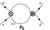
Figure 2: Two diagrams contributing to $\mathrm{|\Delta S|\!=\!2}$-transitions in the effective five- and four-quark theory. The crosses denote insertions of different species of local $\mathrm{|\Delta S|\!=\!1}$-operators.

 

The comparison of the Green’s functions obtained from the full SM lagrangian and the ones derived from (4) allows to fix the values of the Wilson coefficients $C_{k}\!\left(\mu_{tW}\right)$ and $\tilde{C}_{l}\!\left(\mu_{tW}\right)$. The scale $\mu_{tW}$ being of the order of $M_{W}$, $m_{t}$ ensures that there will be no large logarithms in $C_{k}\!\left(\mu_{tW}\right)$ and $\tilde{C}_{l}\!\left(\mu_{tW}\right)$, which therefore can be reliably calculated in ordinary perturbation theory.

The next step is to evolve the Wilson coefficients $C_{k}\!\left(\mu_{tW}\right)$, $\tilde{C}_{l}\!\left(\mu_{tW}\right)$ down to some scale $\mu_{c}=O\!\left(m_{c}\right)$, thereby summing up the $\ln\left(\mu_{c}/\mu_{tW}\right)$ terms to all orders. To do so, one needs to know the corresponding RG equations. While the scaling of the $\mathrm{|\Delta S|\!=\!1}$-coefficients is quite standard, the evolution of the $\mathrm{|\Delta S|\!=\!2}$-coefficients is modified due to the presence of diagrams containing two insertions of $\mathrm{|\Delta S|\!=\!1}$-operators (see Fig. 2). From $\mu\!\frac{d}{d\mu}{\mathcal{L}}_{\mathrm{eff}}^{\mathrm{|\Delta S|\!=\!2}}\!=\!0$ follows:

$$\mu\!\frac{d}{d\mu}\tilde{C}_{k}\!\left(\mu\right)=\tilde{\gamma}_{k^{\prime}k}\tilde{C}_{k^{\prime}}\!\left(\mu\right)+\tilde{\gamma}_{ij,k}C_{i}\!\left(\mu\right)C_{j}\!\left(\mu\right).$$ (5)

In addition to the usual homogeneous differential equation for $\tilde{C}_{l}$ an inhomogenity has emerged. The overall divergence of diagrams with double insertions has been translated into an anomalous dimension tensor $\tilde{\gamma}_{ij,k}$, which is a straightforward generalization of the usual anomalous dimension matrices $\gamma_{ij}$ ($\tilde{\gamma}_{ij}$). The special structure of the operator basis relevant for the calculation of $\eta_{3}$ allows for a very compact solution of (5) $\!{}^{{\bf?}}$.

Finally, at the factorization scale $\mu_{c}$ one has to integrate out the charm-quark from the theory. The effective three-flavour lagrangian obtained in that way already resembles the structure of (1), The only operator left over is $\tilde{Q}_{S2}$. Double insertions no longer contribute, they are suppressed with positive powers of light quark masses.

We want to emphasize that throughout the calculation one has to be very careful about the choice of the operator basis. It contains several sets of unphysical operators. Certainly the most important class of these operators are the so-called evanescent operators. Their precise definition introduces a new kind of scheme-dependence in intermediate results, e.g. anomalous dimensions and matching conditions. This scheme-dependence of course cancels in physical observables. Evanescent operators have been studied in great detail in $\!{}^{{\bf?}}$.

1.3 Numerical Results for $\eta_{3}^{\star}$

The numerical analysis shows $\eta_{3}^{\star}$ being only mildly dependent on the physical input variables $m_{c}^{\star}$, $m_{t}^{\star}$ and $\Lambda_{\scriptscriptstyle\overline{\mathrm{MS}}}$ what allows us to treat $\eta_{3}^{\star}$ essentially as a constant in phenomenological analyses.

More interesting is $\eta_{3}^{\star}$’s residual dependence on the factorization scales $\mu_{c}$ and $\mu_{tW}$. In principle $\eta_{3}^{\star}$ should be independent of these scales, all residual dependence is due to the truncation of the perturbation series. We may use this to determine something like a “theoretical error”.

The situation is very nice with respect to the variation of $\mu_{tW}$. Here the inclusion of the NLO corrections reduces the scale-dependence drastically compared to the LO. For the interval $M_{W}\leq\mu_{tW}\leq m_{t}$ we find a variation of less than 3% in NLO compared to the 12% of the LO.

The dependence of $\eta_{3}^{\star}$ on $\mu_{c}$ has been reduced in NLO compared to the LO analysis. It is displayed in Fig. 3. This variation is the source of the error of $\eta_{3}^{\star}$ quoted in Table 1.

 

Figure 3: The variation of $\eta_{3}^{\star}$ with respect to the factorization scale $\mu_{c}$, where the charm-quark gets integrated out.

 

2 The 1996 Phenomenology of $\left|\varepsilon_{\mathrm{K}}\right|$

The first phenomenological analysis using the full NLO result of the $\mathrm{|\Delta S|\!=\!2}$-hamiltonian has been done in $\!{}^{{\bf?}}$. Here we present a 1996 update.

2.1 Input Parameters

Let us first recall our knowledge of the CKM matrix as reported at this conference $\!{}^{{\bf?}}$:

$$\left|V_{cb}\right| = 0.040\pm 0.003,$$ (6a)

$$\left|V_{ub}/V_{cb}\right| = 0.08\pm 0.02.$$ (6b)

Fermilab now provides us with a very precise determination of $m_{t}^{\mathrm{pole}}=175\pm 6\,\mathrm{GeV}$$\!{}^{{\bf?}}$ which translates into the $\overline{\textrm{MS}}$-scheme as $m_{t}^{\star}=167\pm 6\,\mathrm{GeV}$.

There have been given more precise results on $\mathrm{B_{d}^{0}\!-\!\overline{B_{d}^{0}}}\,$-mixing and $\mathrm{B_{s}^{0}\!-\!\overline{B_{s}^{0}}}\,$-mixing $\!{}^{{\bf?}}$:

$$\Delta m_{\mathrm{B_{d}}} = \left(0.464\pm 0.012\pm 0.013\right)ps^{-1},$$ (7a)

$$\Delta m_{\mathrm{B_{s}}} > 9.2ps^{-1}$$ (7b)

We will further use some theoretical input:

$$B_{\mathrm{K}} = 0.75\pm 0.10$$ (8a)

$$f_{\mathrm{B_{d}}}\sqrt{B_{\mathrm{B_{d}}}} = \left(200\pm 40\right)\,\mathrm{MeV},$$ (8b)

$$\frac{f_{\mathrm{B_{s}}}\sqrt{B_{\mathrm{B_{s}}}}}{f_{\mathrm{B_{d}}}\sqrt{B_{\mathrm{B_{d}}}}} = 1.15\pm 0.05.$$ (8c)

(8b) and(8c) are from quenched lattice QCD, the latter may go up by 10% due to unquenching $\!{}^{{\bf?}}$.

The other input parameters we take as in $\!{}^{{\bf?}}$.

2.2 Results

In extracting information about the still unknown elements of the CKM matrix we still get the strongest restrictions from unitarity and $\varepsilon_{\mathrm{K}}$:

$$\left|\varepsilon_{\mathrm{K}}\right|=\frac{1}{\sqrt{2}}\left[\frac{{\mathrm{Im}\,}\left\langle\mathrm{K^{0}}\right|H^{\mathrm{|\Delta S|\!=\!2}}\left|\overline{\mathrm{K^{0}}}\right\rangle}{\Delta m_{\mathrm{K}}}+\xi\right].$$ (9)

Here $\xi$ denotes some small quantity related to direct CP/ contributing about 3% to $\varepsilon_{\mathrm{K}}$. The key input parameters entering (9) are $V_{cb}$, $|V_{ub}/V_{cb}|$, $m_{t}^{\star}$ and $B_{\mathrm{K}}$

One may use (9) to determine lower bounds on one of the four key input parameters as functions of the other three. In Fig. 4 the currently most interesting lower bound curve which was invented in $\!{}^{{\bf?}}$ is displayed.

 

Figure 4: The lower-bound curves for $|V_{ub}/V_{cb}|$ as a function of $V_{cb}$ for different values of the key input parameters $m_{t}^{\star}$ and $B_{\mathrm{K}}$.

 

Further we are interested in shape of the unitarity triangle, i.e. the allowed values of the top corner $\left(\bar{\rho},\bar{\eta}\right)$

$$\bar{\rho}+i\bar{\eta}=-V_{ud}V_{ub}^{*}/V_{cd}V_{cb}^{*}.$$ (10)

Here, in addition to (9), we take into account the constraint from $\mathrm{B_{d}^{0}\!-\!\overline{B_{d}^{0}}}\,$-mixing

$$\Delta m_{\mathrm{B_{d}}}=\left|V_{td}\right|^{2}\left|V_{ts}\right|^{2}\frac{G_{\mathrm{\!\scriptscriptstyle F}}^{2}}{6\pi^{2}}\eta_{\mathrm{B}}m_{\mathrm{B}}B_{\mathrm{B_{d}}}f_{\mathrm{B_{d}}}^{2}M_{W}^{2}S\!\left(x_{t}\right)$$ (11)

and $\mathrm{B_{s}^{0}\!-\!\overline{B_{s}^{0}}}\,$-mixing

$$\Delta m_{\mathrm{B_{s}}}=\Delta m_{\mathrm{B_{d}}}\cdot\frac{\left|V_{ts}\right|^{2}}{\left|V_{td}\right|^{2}}\cdot\frac{m_{\mathrm{B_{d}}}f_{\mathrm{B_{d}}}^{2}B_{\mathrm{B_{d}}}}{m_{\mathrm{B_{s}}}f_{\mathrm{B_{s}}}^{2}B_{\mathrm{B_{s}}}}.$$ (12)

The allowed region for $\left(\bar{\rho},\bar{\eta}\right)$ depends strongly on the treatment of the errors. We use the following procedure: first we apply (9) to find the CKM phase $\delta$ of the standard parametrization from the input parameters, which are scanned in an 1$\sigma$ ellipsoid of their errors. Second, we check the consistency of the obtained phases $\delta$ with $\mathrm{B_{d}^{0}\!-\!\overline{B_{d}^{0}}}\,$-mixing (11). Here we treat the errors in are fully conservative way. Last we apply the constraint from lower limit on $\Delta m_{\mathrm{B_{s}}}$ (12). This constraint is very sensitive to the value of the flavour-SU(3) breaking term $f_{\mathrm{B_{s}}}\sqrt{B_{\mathrm{B_{s}}}}/f_{\mathrm{B_{d}}}\sqrt{B_{\mathrm{B_{d}}}}$. Using the quenched lattice QCD value (8c) one finds the allowed values of $\left(\bar{\rho},\bar{\eta}\right)$ as displayed in Fig. 5.

 

Figure 5: The allowed values of $\left(\bar{\rho},\bar{\eta}\right)$. The outer contour is obtained solely from $\left|\varepsilon_{\mathrm{K}}\right|$ and unitarity, the medium one takes into account $\mathrm{B_{d}^{0}\!-\!\overline{B_{d}^{0}}}\,$-mixing , the inner curve $\mathrm{B_{s}^{0}\!-\!\overline{B_{s}^{0}}}\,$-mixing  (7b) using the quenched lattice value (8c) for illustrative reasons. If one would use a 10% higher value for the flavour SU(3) breaking as expected for an unquenched calculation no effect is visible for the current limit (7b).

 

If one would increase $f_{\mathrm{B_{s}}}\sqrt{B_{\mathrm{B_{s}}}}/f_{\mathrm{B_{d}}}\sqrt{B_{\mathrm{B_{d}}}}$ by 10% as expected for an unquenched calculation, no effect is visible for the current limit (7b). This can be read off from Fig. 6, where we plot the fraction of area cut out from the allowed region of $\left(\bar{\rho},\bar{\eta}\right)$ by the $\Delta m_{\mathrm{B_{s}}}$ constraint as a function of $\Delta m_{\mathrm{B_{s}}}$.

 

Figure 6: The fraction of the allowed area for $\left(\bar{\rho},\bar{\eta}\right)$ which is excluded by the constraint from $\mathrm{B_{s}^{0}\!-\!\overline{B_{s}^{0}}}\,$-mixing  as a function of $\Delta m_{\mathrm{B_{s}}}$. The curve labelled “quenched” is obtained using (8c), the line labelled “unquenched (est.)” uses a 10% larger value.

 

From Fig. 5 we read off the allowed ranges of the parameters describing the unitarity triangle:

$$\begin{array}[]{c}40^{\circ}\leq\alpha\leq 101^{\circ},\quad 57^{\circ}\leq\gamma\leq 127^{\circ},\\ 0.42\leq\sin\!\left(2\beta\right)\leq 0.79\\ -0.20\leq\bar{\rho}\leq 0.22,\quad 0.25\leq\bar{\eta}\leq 0.43.\end{array}$$ (13)

References

References

• [1] S. Herrlich and U. Nierste, The Complete $\mathrm{|\Delta S|\!=\!2}$-Hamiltonian in the Next-To-Leading Order, Nucl. Phys. B, in press; preprint hep-ph/9604330, DESY 96-048, TUM-T31-86/96.
• [2] S. Herrlich and U. Nierste, Phys. Rev. D52 (1995) 6505.
• [3] F. J. Gilman and M. B. Wise, Phys. Rev. D27 (1983) 1128.
• [4] A. J. Buras, M. Jamin and P. H. Weisz, Nucl. Phys. B347 (1990) 491.
• [5] S. Herrlich and U. Nierste, Nucl. Phys. B419 (1994) 292.
• [6] S. Herrlich and U. Nierste, Nucl. Phys. B455 (1995) 39.
• [7] L. Gibbons, plenary sessions, these proceedings.
• [8] P. Tipton, plenary sessions, these proceedings.
• [9] J. Flynn, plenary sessions, these proceedings.