Perturbative QCD corrections to inclusive lepton distributions from semileptonic $b\rightarrow c\tau\bar{\nu}_{\tau}$ decays

Perturbative corrections of the order of $\alpha_{s}$ to inclusive double differential lepton distribution from $b$ quark decay are considered. A perturbative correction to the charged lepton energy spectrum has been calculated for an arbitrary charged lepton mass. The perturbative contribution suppresses the partial rate but almost does not change the shape of energy distribution. Applications of our result to semileptonic B meson decays are briefly discussed.

I Introduction

The precise determination of weak mixing angles $V_{cb}$ and $V_{ub}$ is a demanding task. In spite of progress in this field they still remain ones of the worse known parameters of the Standard Model. The uncertainties which appear here are both of an experimental and theoretical origin. The relatively large theoretical errors mainly reflect the lack of quantitative knowledge about the structure of hadrons and QCD higher order perturbative corrections to the amplitudes of weak decays of $b$ quarks. The most valuable source of information about the weak mixing angles are the semileptonic decays of $B$ and $\bar{B}$ mesons. The leptons in the final state do not interact strongly and the process is less affected by unknown QCD effects than a hadronic decay. Furthermore pseudoscalar $B$ mesons are the simplest bottom hadrons. The $b$ quark mass is about 5 GeV and thus it exceeds roughly ten times typical energy scales which characterize the infrared dynamics in the hadrons. Moreover the presence of this mass justifies the perturbative treatment of most of the processes involving the $b$ quark. The simple facts have given rise to a quantitative description of dynamics of hadrons containing heavy quarks (Heavy Quark Effective Theory [1, 2, 3, 4, 5, 6]). In the framework of HQET many observables describing heavy hadrons may be expressed as a power series in $1/m_{b}$. In particular it was shown in Ref. [7], that the inclusive lepton distributions from a bottom hadron decay may be treated in such a way. It follows from the operator product expansion (OPE) that a matrix elements which should be evaluated to derive the distributions may be expanded into a series of local operators characterizing the decaying bound state. The very advantage of this approach is that subsequent unknown non-perturbative matrix elements are suppressed by increasing powers of $m_{b}$. The leading term corresponds to a parton contribution to the process. As argued in Ref. [7] the next-to-leading term vanishes. The $1/m_{b}^{2}$ corrections have been calculated by for a case of massless [8, 9] and [10, 11, 12] massive lepton. Recently also the third order terms have become known [13].

The first order perturbative QCD corrections to the inclusive lepton distributions in a process of decay: $b\rightarrow ql\bar{\nu}$ are as important as the HQET corrections for the corresponding $B$ decay. They have been evaluated [14, 15] for the vanishing lepton mass. In the case of a non-zero lepton mass only a differential distribution of the lepton pair invariant mass is known to the first order in strong coupling constant [16]. In the present article we present our recent calculation of the first order QCD correction to the double differential inclusive lepton distribution from $b$ decay with a massive lepton in the final state. The complete analytical result and details of the calculation will be published elsewhere [17]. Here we give results for the perturbative correction to the $\tau$ lepton energy spectrum which has been obtained by numerical integration of this double differential distribution.

II Kinematical variables

The purpose of this section is to define the kinematical variables which are used in this paper. We describe also the constraints imposed on these variables for three and four-body decays of the heavy quark.

The calculation is performed in the rest frame of the decaying $b$ quark. Since the first order perturbative QCD corrections to the inclusive process are taken into account, the final state can consist either of produced quark $c$, lepton $\tau$ and $\tau$ anti-neutrino or of the three particles and a real gluon. The four-momenta of the particles are denoted in the following way: $Q$ for $b$ quark, $q$ for $c$ quark, $\tau$ for the charged lepton, $\nu$ for the corresponding anti-neutrino and $G$ for the real gluon. By the assumption that all the particles are on-shell, the squares of their four-momenta are equal to the squares of masses:

$$Q^{2}=m_{b}^{2},\qquad q^{2}=m_{c}^{2},\qquad\tau^{2}=m_{\tau}^{2},\qquad\nu^{2}=G^{2}=0.$$ (1)

The four-vectors $P=q+G$ and $W=\tau+\nu$ characterize the quark–gluon system and the virtual $W$ boson respectively. We define a set of variables scaled in the units of mass of heavy quark $m_{b}$:

$$\varrho={m_{c}^{2}\over m_{b}^{2}},\qquad\eta={m_{\tau}^{2}\over m_{b}^{2}},\qquad x={2E_{\tau}\over m_{b}^{2}},\qquad t={W^{2}\over m_{b}^{2}},\qquad z={P^{2}\over m_{b}^{2}}.$$ (2)

We introduce light-cone variables describing the charged lepton:

$$\tau_{\pm}={1\over 2}\left(x\pm\sqrt{x^{2}-4\eta}\right)$$ (3)

The system of $c$ quark and real gluon is characterized by the following quantities:

$$P_{0}(z) = {1\over 2}(1-t+z),$$ (4)

$$P_{3}(z) = \sqrt{P_{0}^{2}-z}={1\over 2}[1+t^{2}+z^{2}-2(t+z+tz)]^{1/2},$$ (5)

$$P_{\pm}(z) = P_{0}(z)\pm P_{3}(z),$$ (6)

$${\cal Y}_{p}(z) = {1\over 2}\ln{P_{+}(z)\over P_{-}(z)}=\ln{P_{+}(z)\over\sqrt{z}}$$ (7)

where $P_{0}(z)$ and $P_{3}(z)$ are the energy and length of the momentum vector of the system in $b$ quark rest frame, ${\cal Y}_{p}(z)$ is the corresponding rapidity. Similarly for virtual $W$:

$$W_{0}(z) = {1\over 2}(1+t-z),$$ (9)

$$W_{3}(z) = \sqrt{W_{0}^{2}-t}={1\over 2}[1+t^{2}+z^{2}-2(t+z+tz)]^{1/2},$$ (10)

$$W_{\pm}(z) = W_{0}(z)\pm W_{3}(z),$$ (11)

$${\cal Y}_{w}(z) = {1\over 2}\ln{W_{+}(z)\over W_{-}(z)}=\ln{W_{+}(z)\over\sqrt{t}},$$ (12)

¿From kinematical point of view the three body decay is a special case of the four body one with vanishing gluon four-momentum, what is equivalent to $z=\varrho$. It is convenient to use in this case the following variables:

$\displaystyle p_{0}=P_{0}(\varrho)={1\over 2}(1-t+\varrho),\qquad p_{3}=P_{3}(\varrho)=\sqrt{p_{0}^{2}-\varrho},$

$\displaystyle p_{\pm}=P_{\pm}(\varrho)=p_{0}\pm p_{3},\qquad w_{\pm}=W_{\pm}(\varrho)=1-p_{\mp}.$

$$Y_{p}={\cal Y}_{p}(\varrho)={1\over 2}\ln{p_{+}\over p_{-}},\qquad Y_{w}={\cal Y}_{w}(\varrho)={1\over 2}\ln{w_{+}\over w_{-}}.$$ (14)

We express also the scalar products which appear in the calculation by the variables $x$, $t$ and $z$:

$$\begin{array}[]{ll}Q\!\cdot\!P\,={1\over 2}(1+z-t)&\tau\!\cdot\!\nu\,={1\over 2}(t-\eta)\\ Q\!\cdot\!\nu\,={1\over 2}(1-z-x+t)&\tau\!\cdot\!P\,={1\over 2}(x-t-\eta)\\ Q\!\cdot\!\tau\,={1\over 2}x&\nu\!\cdot\!\tau\,={1\over 2}(1-x-z+\eta)\\ \end{array}$$ (15)

All of the written above products are scaled in the units of the mass of $b$ quark.

The allowed ranges of $x$ and $t$ for the three-body decay are given by following inequalities:

$$2\sqrt{\eta}\leq x\leq 1+\eta-\varrho=x_{max},\qquad$$ (16)

$$t_{1}=\tau_{-}\left(1-{\varrho\over 1-\tau_{-}}\right)\leq t\leq\tau_{+}\left(1-{\varrho\over 1-\tau_{+}}\right)=t_{2}$$ (17)

(a region A). In the case of the four-body process the available region of the phase space is larger than the region A. The additional, specific for the four body decay area of the phase space is denoted as a region B. Its boundaries are given by the formulae:

$$2\sqrt{\eta}\leq x\leq x_{max},\qquad\eta\leq t\leq t_{1}$$ (18)

We remark, that if the charged lepton mass tends to zero than the region B vanishes.

One can also parameterize the kinematical boundaries of $x$ as functions of $t$. In this case we obtain for the region A:

$$\eta\leq t\leq(1-\sqrt{\varrho})^{2},\qquad w_{-}+{\eta\over w_{-}}\leq x\leq w_{+}+{\eta\over w_{+}},$$ (19)

and for the region B:

$$\eta\leq t\leq\sqrt{\eta}\left(1-{\varrho\over 1-\sqrt{\eta}}\right),\qquad 2\sqrt{\eta}\leq x\leq w_{-}+{\eta\over w_{-}}.$$ (20)

The upper limit of the mass squared of the $c$-quark — gluon system is in both regions given by

$$z_{max}=(1-\tau_{+})(1-t/\tau_{+}),$$ (21)

whereas the lower limit depends on a region:

$$z_{min}=\left\{\begin{array}[]{ll}\varrho&\mbox{\rm in the region A}\\ (1-\tau_{-})(1-t/\tau_{-})&\mbox{\rm in the region B.}\\ \end{array}\right.$$ (22)

III Evaluation of the QCD corrections

The QCD corrected differential rate for $b\rightarrow c+\tau^{-}+\bar{\nu}$ reads:

$$d\Gamma=d\Gamma_{0}+d\Gamma_{1,3}+d\Gamma_{1,4},$$ (23)

where

$$d\Gamma_{0}=G_{F}^{2}m_{b}^{5}|V_{CKM}|^{2}{\cal M}_{0,3}^{-}d{\cal R}_{3}(Q;q,\tau,\nu)/\pi^{5}$$ (24)

in Born approximation,

$$d\Gamma_{1,3}={2\over 3}\alpha_{s}G_{F}^{2}m_{b}^{5}|V_{CKM}|^{2}{\cal M}_{1,3}^{-}d{\cal R}_{3}(Q;q,\tau,\nu)/\pi^{6}$$ (25)

comes from the virtual gluon contribution and

$$d\Gamma_{1,4}={2\over 3}\alpha_{s}G_{F}^{2}m_{b}^{5}|V_{CKM}|^{2}{\cal M}_{1,4}^{-}d{\cal R}_{4}(Q;q,\tau,\nu)/\pi^{7}$$ (26)

describes a real gluon emission. $V_{CKM}$ is the Cabbibo–Kobayashi–Maskawa matrix element associated the $b$ to $c$ or $u$ quark weak transition. Lorentz invariant $n$-body phase space is defined as

$$d{\cal R}_{n}(P;p_{1},\ldots,p_{n})=\delta^{(4)}(P-\sum p_{i})\prod_{i}{d^{3}{\bf p}_{i}\over 2E_{i}}$$ (27)

In Born approximation the rate for the decay into three body final state is proportional to the expression

$${\cal M}_{0,3}^{-}=F_{0}(x,t)=4q\!\cdot\!\tau\;Q\!\cdot\!\nu\;=(1-\varrho-x+t)(x-t-\eta),$$ (28)

where the quantities describing the $W$ boson propagator are neglected. Interference between virtual gluon exchange and Born amplitude yields:

$${\cal M}_{1,3}^{-} = -[\;q\!\cdot\!\tau\;Q\!\cdot\!\nu\;H_{0}+\varrho\;Q\!\cdot\!\nu\;Q\!\cdot\!\tau\;H_{+}+\;q\!\cdot\!\nu\;q\!\cdot\!\tau\;H_{-}+$$ (30)

$$+{1\over 2}\varrho\;\nu\!\cdot\!\tau\;(H_{+}+H_{-})+{1\over 2}\eta\varrho\;Q\!\cdot\!\nu\;(H_{+}-H_{-}+H_{L})-{1\over 2}\eta\;q\!\cdot\!\nu\;H_{L}],$$

where

$$H_{0} = 4(1-Y_{p}p_{0}/p_{3})\ln\lambda_{G}+(2p_{0}/p_{3})\left[\mbox{Li}_{2}\left(1-{p_{-}w_{-}\over p_{+}w_{+}}\right)\right.$$ (34)

$$-\left.\mbox{Li}_{2}\left(1-{w_{-}\over w_{+}}\right)-Y_{p}(Y_{p}+1)+2(\ln\sqrt{\varrho}+Y_{p})(Y_{w}+Y_{p})\right]$$

$$+[2p_{3}Y_{p}+(1-\varrho-2t)\ln\sqrt{\varrho}]/t+4,$$

$$H_{\pm} = {1\over 2}[1\pm(1-\varrho)/t]Y_{p}/p_{3}\pm{1\over t}\ln\sqrt{\varrho},$$ (35)

$$H_{L} = {1\over t}(1-\ln\sqrt{\varrho})+{1-\varrho\over t^{2}}\ln\sqrt{\varrho}+{2\over t^{2}}Y_{p}p_{3}+{\varrho\over t}{Y_{p}\over p_{3}}.$$ (36)

In ${\cal M}_{1,3}^{-}$ infrared divergences are regularized by a small mass of gluon denoted by $\lambda_{G}$. According to Kinoshita–Lee–Naunberg theorem, the infrared divergent part should cancel with the infrared contribution of the four-body decay amplitude integrated over suitable part of the phase space.

The rate from real gluon emission is proportional to

$${\cal M}^{-}_{1,4}={{\cal B}^{-}_{1}\over(Q\!\cdot\!G)^{2}}-{{\cal B}^{-}_{2}\over Q\!\cdot\!G\;P\!\cdot\!G}+{{\cal B}^{-}_{3}\over(P\!\cdot\!G)^{2}},$$ (38)

where

$${\cal B}_{1}^{-} = \,q\!\cdot\!\tau\;[\,Q\!\cdot\!\nu\;(Q\!\cdot\!G\,-1)+\,G\!\cdot\!\nu\,-\,Q\!\cdot\!\nu\;Q\!\cdot\!G\,+\,G\!\cdot\!\nu\;Q\!\cdot\!G\,],$$ (39)

$${\cal B}_{2}^{-} = \,q\!\cdot\!\tau\;[\,G\!\cdot\!\nu\;Q\!\cdot\!q\,-\,q\!\cdot\!\nu\;Q\!\cdot\!G\,+\,Q\!\cdot\!\nu\;(\,q\!\cdot\!G\,-\,Q\!\cdot\!G\,-2\,q\!\cdot\!Q\,)]+$$ (41)

$$+\,Q\!\cdot\!\nu\;(\,Q\!\cdot\!\tau\;q\!\cdot\!G\,-\,G\!\cdot\!\tau\;q\!\cdot\!Q\,),$$

$${\cal B}_{3}^{-} = Q\!\cdot\!\nu\;(\,G\!\cdot\!\tau\;q\!\cdot\!G\,-\varrho\;\tau\!\cdot\!P\,).$$ (42)

Integrating and adding all the contributions one arrives at the following double differential distribution of leptons:

$${d\Gamma\over dx\,dt}=\left\{\begin{array}[]{ll}12\Gamma_{0}\left[F_{0}(x,t)-{2\alpha_{s}\over 3\pi}F_{1}^{A}(x,t)\right]&\mbox{for $(x,t)$ in A},\\ 12\Gamma_{0}{2\alpha_{s}\over 3\pi}F_{1}^{B}(x,t)&\mbox{for $(x,t)$ in B}\\ \end{array}\right.$$ (44)

where

$$\Gamma_{0}={G_{F}^{2}m_{b}^{5}\over 192\pi^{3}}|V_{CKM}|^{2},$$ (45)

$$F_{0}(x,t)=(1-\varrho-x+t)(x-t-\eta),$$ (46)

and the functions $F_{1}^{A}(x,t)$, $F_{1}^{B}(x,t)$ describe the perturbative correction in the regions $A$ and $B$. Explicite formulae for $F_{1}^{A}(x,t)$ and $F_{1}^{B}(x,t)$ will be given in [17]. The factor of 12 in the formula (44) is introduced to meet widely used [10, 16, 20] convention for $F_{0}(x)$ and $\Gamma_{0}$.

The obtained results were tested by comparison with earlier calculations. One of the cross checks was arranged by fixing the mass of the produced lepton to zero. Our results are in this limit algebraically identical with those for the massless charged lepton [14, 15]. On the other hand one can numerically integrate the calculated double differential distribution over $x$, with the limits given by the kinematical boundaries:

$$\int_{2\sqrt{\eta}}^{w_{+}+\eta/w_{+}}{d\Gamma\over dx\,dt}(x,t;\varrho,\eta)={d\Gamma\over dt}(t;\varrho,\eta)$$ (47)

Obtained in such a way differential distribution of $t$ agrees with recently published [16] analytical formula describing this distribution. This test is particularly stringent because one requires two functions of three variables ($t,\varrho$ and $\eta$) to be numerically equal for any values of the arguments. We remark, that for higher values of $t$ only the region A contributes to the integral (47) and for lower values of $t$ both regions A and B contribute. This feature of the test is very helpful — the formulae for $F_{1}(x,t)$, which are different for the regions A and B can be checked separately.

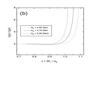
FIG. 1.: (a) The distributions $f_{0}(x)$, $f_{1}(x)$ and (b) the ratio $f_{1}(x)/f_{0}(x)$ for the pole mass of the $b$ quark $m_{b}=4.5$ GeV (dotted), $m_{b}=4.75$ GeV (solid) and $m_{b}=5.0$ GeV (dashed).

IV Differential distribution of $\tau$ energy

The point of interest to check how the QCD corrections change energy spectrum of the charged lepton. This aim may be reached by integration of the double differential lepton distribution over the lepton pair invariant mass:

$${d\Gamma\over dx}=\int_{\eta}^{t_{2}}{d\Gamma\over dx\,dt}\,dt,$$ (48)

where $t_{2}$ is the upper kinematical boundary for $t$ given the formula (19). The decomposition of the resulting distribution into the Born term and the perturbative QCD correction yields in a natural way definitions of functions $f_{0}(x)$ and $f_{1}(x)$:

$${d\Gamma\over dx}=12\Gamma_{0}\left[f_{0}(x)-{2\alpha_{s}\over 3\pi}f_{1}(x)\right].$$ (49)

The analytical formula for $f_{0}(x)$ reads

$$f_{0}(x) = 2\sqrt{x^{2}-4\eta}\left\{x_{0}^{3}[x^{2}-3x(1+\eta)+8\eta]+\right.$$ (51)

$$\hskip 100.0pt\left.+x_{0}^{2}[-3x^{2}+6x(1+\eta)-12\eta]\right\},$$

where following [10] we introduced

$$x_{0}=1-\varrho/(1+\eta-x).$$ (53)

An equivalent expression for $f_{0}(x)$ is

$$f_{0}(x) = {1\over 6}x\sqrt{x^{2}-4\eta}\left(\frac{x_{max}-x}{1+\eta-x}\right)^{2}[3(1+\eta)-2x+\varrho-4\eta/x+$$ (55)

$$\hskip 105.0pt+2\varrho(1+\eta-4\eta/x)/(1+\eta-x)],$$

where $x_{max}$ is given by (16). The latter formula clearly exhibits the behavior of $f_{0}(x)$ for $x$ close to the upper kinematical limit.

The integration of $F^{A,B}_{1}(x,t)$ was performed numerically for different masses of $b$-quark with fixed $m_{b}-m_{c}=3.4$ GeV and $m_{\tau}=1.777$ GeV. The functions $f_{0}(x)$ and $f_{1}(x)$ for $m_{b}=4.75$ GeV are plotted on Fig. 1a and the ratios $f_{1}(x)/f_{0}(x)$ for three different realistic values of $m_{b}$ are plotted on Fig. 1b. As can be easily seen the ratios have logarithmic singularities at the upper end of the spectra. Such a behavior would lead to a inconsistence. The standard solution to problems of this kind is an exponentiation which yields well known Sudakov form factor [18]. Far from the end point the ratio of the correction term to the leading one is almost constant and close to 2. It means that the perturbative correction changes rather the normalization than the shape of lepton energy distribution.

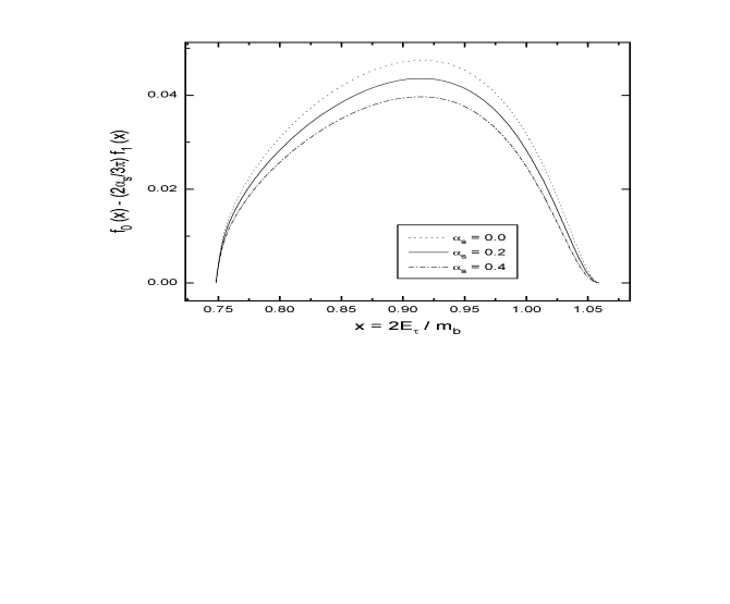
FIG. 2.: The QCD corrected $\tau$ lepton spectrum from the $b$ quark decay for different values of $\alpha_{s}$. The mass of $b$ quark is chosen as 4.75 GeV.

The obtained distributions of the scaled charged lepton energy for $m_{b}=4.75$ GeV with and without perturbative QCD corrections are shown in Fig. 2. The strong coupling constant was chosen as $0.2$ and $0.4$ since the energy scale for this process in not known until the second order QCD corrections are evaluated. The value of $\alpha_{s}$ for this decay is expected to lay between the two numbers.

The knowledge of perturbative corrections to lepton energy is essential for fixing HQET parameters, especially $\lambda_{1}$ and $\bar{\Lambda}$ [8, 9]. Especially analysis of moments of the lepton energy spectrum and other quantities involving integration over the energy distribution appeared particularly valuable for this purpose [19] as was earlier suggested in Refs. [16, 20].

V Conclusions

The first order QCD corrections to the double differential inclusive lepton distributions from $b$ quark semileptonic decay have been calculated for a massive fermion in the final state. Non-trivial cross checks of the final the result have been performed. We remark that including a real gluon radiation on the parton level yields a increase of the phase space available in the decay process. The QCD corrected $\tau$ energy spectrum has been obtained. The effect of the correction may be estimated as about 10% of the magnitude of uncorrected distributions.

The presented above results can be utilized to improve an analysis of semileptonic decays of beauty hadrons with a $\tau$ in the final state. Thus the values of involved weak mixing angles may be fixed more exactly. The decrease of theoretical uncertainty increases the sensitivity to hypothetic deviations from the Standard Model [21, 22, 23] which should have to be particularly distinct in the case of the heaviest family. The better understanding of the perturbative QCD effects allows one to perform more stringent tests of HQET predictions [10, 11, 12] and narrow the error bars for HQET parameters. Moreover one can extract more precisely some information about masses of quarks and strong coupling constant from the data. Finally, the process that we considered may appear a background for other processes so precise theoretical knowledge about the process is valuable. At present however the statistics of measured $b\rightarrow c(u)\tau\bar{\nu}_{\tau}$ transitions is rather low and ten-percent effects are not seen. Probably the application of provided here formulae to the expected data from $B$-factories will be really fruitful.

REFERENCES

- [1] M. Voloshin and M. Shifman, Sov. J. Nucl. Phys. 45 (1987) 292; 47 (1988) 511.
- [2] H.D. Politzer and M.B. Wise, Phys. Lett. B206 (1988) 681; B208 (1988) 504.
- [3] N. Isgur and M.B. Wise, Phys. Lett. B232 (1989) 113; B237 (1990) 527.
- [4] E. Eichten and B. Hill, Phys. Lett B234 (1990) 511.
- [5] B. Grinstein, Nucl. Phys. B339 (1990) 253.
- [6] H. Georgi, Phys. Lett. B240 (1990) 447.
- [7] J. Chay, H. Georgi and B. Grinstein, Phys. Lett. B247 (1990) 399.
- [8] I.I. Bigi et al, Phys. Lett. B293 (1992) 430 [(E) ibid. B297 (1993) 477]; I.I. Bigi et al., Phys. Rev. Lett. 71 (1993) 496.
- [9] A.V. Manohar and M.B. Wise, Phys. Rev. D49 (1994) 1310; B. Blok et al., Phys. Rev. D49 (1994) 3356 [(E) ibid. D50 (1994) 3572; T. Mannel, Nucl. Phys. B413 (1994) 396.
- [10] A.F. Falk, Z. Ligeti, M. Neubert and Y. Nir, Phys. Lett 326 (1994) 145.
- [11] L. Koyrakh, Phys. Rev. D49 (1994) 3379; L. Koyrakh, PhD. Thesis, hep/ph9607443.
- [12] S. Balk, J.G. Körner, D. Pirjol and K. Schilcher, Z. Phys. C64 (1994) 37.
- [13] M. Gremm, A. Kapustin, CALT-68-2043, hep/ph/9603448.
- [14] M. Jeżabek, H. Kühn, Nucl. Phys. B320 (1989) 20.
- [15] A. Czarnecki, M. Jeżabek, Nucl. Phys. B427 (1994) 3.
- [16] A. Czarnecki, M. Jeżabek, H. Kühn, Phys. Lett. B346 (1995) 335.
- [17] M. Jeżabek, L. Motyka, in preparation.
- [18] G. Altarelli et al., Nucl. Phys. B208 (1982) 365.
- [19] M. Gremm, A. Kapustin, Z. Ligeti and M.B. Wise, hep/ph9603314.
- [20] M.B. Voloshin, Phys. Rev. D51 (1995) 4934.
- [21] J. Kalinowski, Phys.Lett. B245 (1990) 201.
- [22] Y. Grossman and Z. Ligeti, Phys. Lett. B332 (1994) 373.
- [23] Y. Grossman, H.E. Haber and Y. Nir, Phys. Lett. B357 (1995) 630.