Phenomenology of two Higgs doublet models with flavor changing neutral currents

Abstract

A comprehensive phenomenological analysis of a two Higgs doublet model, with flavor-changing scalar currents at the tree-level, called model III, is presented. Constraints from existing experimental information especially on $\Delta F=2$ processes are systematically incorporated. Constraints emerging from rare $B$-decays, $Z\rightarrow b\bar{b}$, and the $\rho$-parameter are also examined. Experimental implications for $e^{+}e^{-}(\mu^{+}\mu^{-})\rightarrow t\bar{c}+\bar{t}c$, $t\rightarrow c\gamma(Z,g)$, $D^{0}$-$\bar{D}^{0}$, and $B^{0}_{s}$-$\bar{B}^{0}_{s}$ oscillations, and for $e^{+}e^{-}(Z)\rightarrow b\bar{s}+\bar{b}s$ are investigated and experimental effort towards these is stressed. We also emphasize the importance of clarifying the experimental issues pertaining to $Z\rightarrow b\bar{b}$.

I Introduction

Recently we have been examining various issues [1, 2], in a class of two Higgs doublet models (2HDM’s) which allow flavor changing neutral currents (FCNC’s) at the tree level [3, 4, 5, 6, 7]. In this work we want to present a comprehensive analysis which gives the details of the analytical calculations we used and summarize the status of our knowledge regarding this type of 2HDM’s. In particular we will examine the important constraints and derive quantitative bounds on the mass parameters and flavor changing (FC) couplings of the new scalar fields based on existing low energy experiments.

FCNC’s are naturally suppressed in the standard model (SM) because they are forbidden at the tree level. However, at the one loop level, the amplitudes for the Feynman diagrams which generate FC processes tend to increase with virtual quark masses. Due to the large disparity in masses of the up-type quarks, the GIM [8] suppression gets very effectively removed in loops of these (virtual) quarks. Therefore, FC transitions involving a pair of down-type quarks get enhanced, due primarily to the presence of a top-quark in the loop, while FC transitions which involve up-type quarks are usually very small. This motivates the interest in processes like $b\rightarrow s,d\gamma$ instead of $t\rightarrow c\gamma,Z$ or for $K^{0}\!-\!\bar{K}^{0}$ and $B^{0}\!-\!\bar{B}^{0}$ mixing instead of $D^{0}-\bar{D}^{0}$ mixing.

There are many ways in which the extensions of the SM lead to FC couplings at the tree level. For instance, as soon as we go from a theory with one doublet of scalar fields to a theory with two doublets, FCNC’s are generated in the scalar sector of the theory. In this case, couplings such as $tc\gamma$ or $tcZ$ can get enhanced too, in much the same manner as there is an enhancement of $bs\gamma$ in the SM. The interest in this class of implications is obvious: we could have a clear signal of new physics, since the SM prediction for any process involving a $tc\gamma$ or a $tcZ$ vertex is extremely small.

As is well known, a model with tree level FCNC’s will also have many important repercussions for the $\Delta F=2$ mixing processes such as $K^{0}-\bar{K}^{0}$, $B^{0}-\bar{B}^{0}$, and $D^{0}-\bar{D}^{0}$. Indeed the measured size of the mixing amplitude for $K^{0}-\bar{K}^{0}$, known for a very long time, is so small that it places severe restrictions on the FC sector of extended models. This led Glashow and Weinberg [9] to propose an ad hoc discrete symmetry whose sole purpose was to forbid tree-level FCNC’s to appear in models with more than one Higgs doublet. In particular, for the simplest case of 2HDM’s, depending on whether the up-type and down-type quarks couple to the same or to two different scalar doublets leads to two versions of such models, called model I and model II. Both of them share with the SM the distinctive feature that they do not allow tree-level FCNC’s. These models have been extensively studied and a multitude of interesting implications have been discussed in the literature.

Our starting point for investigating tree-level FCNC’s is primarily based on the realization that the top quark may be quite different from the lighter quarks. It may well be that the theoretical prejudice of the non existence of tree level FCNC’s, based on experiments involving the lighter quarks, is not relevant to the top quark. This leads one to formulate a model which allows the possibility of large tree level FCNC’s involving the top quark while it keeps the FCNC’s of the lighter quarks, especially those involving the quarks of the first family, at a negligible level. A rather natural way of implementing this notion is by taking the new scalar FC vertices to be proportional to the masses of the participating quarks at the vertex [3, 4, 5]. A hierarchy is then automatically introduced which enhances the top quark couplings while keeping the couplings of the lighter quarks at some order of magnitude smaller. The compatibility of any such assumption with the many constraints mentioned above clearly needs to be checked and the allowed region of the parameter space determined, in particular, scalar masses and couplings. This type of 2HDM is now referred to as model III [10].

Our first interest in model III was motivated by the idea of looking for top-charm production at an $e^{+}e^{-}$ and/or $\mu^{+}\mu^{-}$ collider [1, 2]. We were intrigued by the possibility of a clear signal for the reaction $e^{+}e^{-}\rightarrow t\bar{c}$ for which the SM prediction is extremely small. The reaction has a distinctive kinematical signature in a very clean environment. These characteristics, which are unique to the lepton colliders, should compensate for the lower statistics one expects compared to those at hadron colliders. In this paper we present the details of our calculations for this important process.

After a brief overview of model III in Sec. II, we will discuss $e^{+}e^{-}\rightarrow t\bar{c}+\bar{t}c$ in Sec. III and present some of the relevant formulae in detail in Appendix B. In Sec. IV we will consider the rare decays $t\rightarrow c\gamma,Z$ and $g$; herein we will also compare our results with those existing in the literature for $t\rightarrow c\gamma$ and $cZ$ in model III. Top-charm production at a $\mu^{+}\mu^{-}$ collider is briefly discussed in Sec. V. In Sec. VI we consider the repercussions of the $\Delta F=2$ mixing processes and extract the constraints that emerge on parameters of model III. Sec. VII discusses the impact of the experimental results for $Br(B\rightarrow X_{s}\gamma)$, the $\rho$-parameter and $Z\rightarrow b\bar{b}$. We then examine in Sec. VIII the physical consequences of the constrained physical model for the $B_{s}^{0}-\bar{B}_{s}^{0}$ oscillations, the flavor-changing $Z$ decay $Z\rightarrow\bar{b}s+b\bar{s}$, and also some rare $B$-decays. Sec. IX offers the outlook and the conclusions.

II The model

A mild extension of the SM with one additional scalar SU(2) doublet opens up the possibility of flavor changing scalar currents (FCSC’s) at the tree level. In fact, when the up-type quarks and the down-type quarks are allowed simultaneously to couple to more than one scalar doublet, the diagonalization of the up-type and down-type mass matrices does not automatically ensure the diagonalization of the couplings with each single scalar doublet. For this reason, the 2HDM scalar potential and Yukawa Lagrangian are usually constrained by an ad hoc discrete symmetry [9], whose only role is to protect the model from FCSC’s at the tree level. Let us consider a Yukawa Lagrangian of the form

$${\cal L}^{(III)}_{Y}=\eta^{U}_{ij}\bar{Q}_{i,L}\tilde{\phi}_{1}U_{j,R}+\eta^{D}_{ij}\bar{Q}_{i,L}\phi_{1}D_{j,R}+\xi^{U}_{ij}\bar{Q}_{i,L}\tilde{\phi}_{2}U_{j,R}+\xi^{D}_{ij}\bar{Q}_{i,L}\phi_{2}D_{j,R}\,+\,h.c.$$ (1)

where $\phi_{i}$, for $i=1,2$, are the two scalar doublets of a 2HDM, while $\eta^{U,D}_{ij}$ and $\xi_{ij}^{U,D}$ are the non-diagonal matrices of the Yukawa couplings. Imposing the following ad hoc discrete symmetry

$$\phi_{1}\rightarrow-\phi_{1}\,\,\,\,\,\,\,\,\,\mbox{and} \,\,\,\,\,\phi_{2}\rightarrow\phi_{2}$$ (2)

$$D_{i}\rightarrow-D_{i}\,\,\,\,\,\,\,\,\,\mbox{and} \,\,\,\,\,U_{i}\rightarrow\mp U_{i}$$ (3)

one obtains the so called model I and model II, depending on whether the up-type and down-type quarks are coupled to the same or to two different scalar doublets respectively [11].

In contrast we will consider the case in which no discrete symmetry is imposed and both up-type and down-type quarks then have FC couplings. For this type of 2HDM, which we will call model III, the Yukawa Lagrangian for the quark fields is as in Eq. (1) and no term can be dropped a priori, see also refs. [7, 1].

For convenience we can choose to express $\phi_{1}$ and $\phi_{2}$ in a suitable basis such that only the $\eta_{ij}^{U,D}$ couplings generate the fermion masses, i.e. such that

$$\langle\phi_{1}\rangle=\left(\begin{array}[]{c}0\\ {v/\sqrt{2}}\end{array}\right)\,\,\,\,,\,\,\,\,\langle\phi_{2}\rangle=0\,\,\,.$$ (4)

The two doublets are in this case of the form

$$\phi_{1}=\frac{1}{\sqrt{2}}\left[\left(\begin{array}[]{c}0\\ v+H^{0}\end{array}\right)+\left(\begin{array}[]{c}\sqrt{2}\,\chi^{+}\\ i\chi^{0}\end{array}\right)\right]\,\,\,\,;\,\,\,\,\phi_{2}=\frac{1}{\sqrt{2}}\left(\begin{array}[]{c}\sqrt{2}\,H^{+}\\ H^{1}+iH^{2}\end{array}\right)\,\,\,.$$ (5)

The scalar Lagrangian in the ($H^{0}$, $H^{1}$, $H^{2}$, $H^{\pm}$) basis is such that[12, 11]:

1. the doublet $\phi_{1}$ corresponds to the scalar doublet of the SM and $H^{0}$ to the SM Higgs field (same couplings and no interactions with $H^{1}$ and $H^{2}$);

2. all the new scalar fields belong to the $\phi_{2}$ doublet;

3. both $H^{1}$ and $H^{2}$ do not have couplings to the gauge bosons of the form $H^{1,2}ZZ$ or $H^{1,2}W^{+}W^{-}$.

However, while $H^{\pm}$ is also the charged scalar mass eigenstate, ($H^{0}$, $H^{1}$, $H^{2}$) are not the neutral mass eigenstates. Let us denote by ($\bar{H}^{0}$, $h^{0}$) and $A^{0}$ the two scalar plus one pseudoscalar neutral mass eigenstates. They are obtained from ($H^{0}$, $H^{1}$, $H^{2}$) as follows

$$\bar{H}^{0} = \left[(H^{0}-v)\cos\alpha+H^{1}\sin\alpha\right]$$ (6)

$$h^{0} = \left[-(H^{0}-v)\sin\alpha+H^{1}\cos\alpha\right]$$ (7)

$$A^{0} = H^{2}$$ (8)

where $\alpha$ is a mixing angle, such that for $\alpha\!=\!0$, ($H^{0}$, $H^{1}$, $H^{2}$) coincide with the mass eigenstates. We find it more convenient to express $H^{0}$, $H^{1}$, and $H^{2}$ as functions of the mass eigenstates, i.e.

$$H^{0} = \left(\bar{H}^{0}\cos\alpha-h^{0}\sin\alpha\right)+v$$ (9)

$$H^{1} = \left(h^{0}\cos\alpha+\bar{H}^{0}\sin\alpha\right)$$ (10)

$$H^{2} = A^{0}\,\,\,.$$ (11)

In this way we may take advantage of the mentioned properties (1), (2), and (3), as far as the calculation of the contribution from new physics goes. In particular, only the $\phi_{1}$ doublet and the $\eta^{U}_{ij}$ and $\eta^{D}_{ij}$ couplings are involved in the generation of the fermion masses, while $\phi_{2}$ is responsible for the new couplings.

After the rotation that diagonalizes the mass matrix of the quark fields, the FC part of the Yukawa Lagrangian looks like

$${\cal L}_{Y,FC}^{(III)}=\hat{\xi}^{U}_{ij}\bar{Q}_{i,L}\tilde{\phi}_{2}U_{j,R}+\hat{\xi}^{D}_{ij}\bar{Q}_{i,L}\phi_{2}D_{j,R}\,+\,h.c.$$ (12)

where $Q_{i,L}$, $U_{j,R}$, and $D_{j,R}$ denote now the quark mass eigenstates and $\hat{\xi}_{ij}^{U,D}$ are the rotated couplings, in general not diagonal. If we define $V_{L,R}^{U,D}$ to be the rotation matrices acting on the up- and down-type quarks, with left or right chirality respectively, then the neutral FC couplings will be

$$\hat{\xi}^{U,D}_{\rm neutral}=(V_{L}^{U,D})^{-1}\cdot\xi^{U,D}\cdot V_{R}^{U,D}\,\,\,.$$ (13)

On the other hand for the charged FC couplings we will have

$$\hat{\xi}^{U}_{\rm charged}\! = \!\hat{\xi}^{U}_{\rm neutral}\cdot V_{\scriptscriptstyle{\rm CKM}}$$ (14)

$$\hat{\xi}^{D}_{\rm charged}\! = \!V_{\scriptscriptstyle{\rm CKM}}\cdot\hat{\xi}^{D}_{\rm neutral}$$ (15)

where $V_{\scriptscriptstyle{\rm CKM}}$ denotes the Cabibbo-Kobayashi-Maskawa matrix. To the extent that the definition of the $\xi^{U,D}_{ij}$ couplings is arbitrary, we can take the rotated couplings as the original ones. Thus, we will denote by $\xi^{U,D}_{ij}$ the new rotated couplings in Eq. (13), such that the charged couplings in Eq. (15) look like $\xi^{U}\cdot V_{\scriptscriptstyle{\rm CKM}}$ and $V_{\scriptscriptstyle{\rm CKM}}\cdot\xi^{D}$. This form of the charged couplings is indeed peculiar to model III: they appear as a linear combination of neutral FC couplings multiplied by some CKM matrix elements. This is an important distinction between model III on the one hand, and models I and II on the other. As we will see in the phenomenological analysis this can have important repercussions for many different physical quantities.

In order to apply to specific processes we have to make some definite ansatz on the $\xi_{ij}^{U,D}$ couplings. Many different suggestions can be found in the literature [3, 4, 5, 1]. In addition to symmetry arguments, there are also arguments based on the widespread perception that these new FC couplings are likely to mainly affect the physics of the third generation of quarks only, in order to be consistent with the constraints coming from $K^{0}\!-\!\bar{K}^{0}$ and $B^{0}\!-\!\bar{B}^{0}$. A natural hierarchy among the different quarks is provided by their mass parameters, and that has led to the assumption that the new FC couplings are proportional to the mass of the quarks involved in the coupling. Most of these proposals are well described by the following equation

$$\xi^{U,D}_{ij}=\lambda_{ij}\,\frac{\sqrt{m_{i}m_{j}}}{v}$$ (16)

which basically coincides with what was proposed by Cheng and Sher [3]. In this ansatz the residual degree of arbitrariness of the FC couplings is expressed through the $\lambda_{ij}$ parameters, which need to be constrained by the available phenomenology. In particular we will see how $K^{0}\!-\!\bar{K}^{0}$ and $B^{0}\!-\!\bar{B}^{0}$ mixings (and to a less extent $D^{0}\!-\!\bar{D}^{0}$ mixing) put severe constraints on the FC couplings involving the first family of quarks. Additional constraints are given by the combined analysis of the $Br(B\rightarrow X_{s}\gamma)$, the $\rho$-parameter, and $R_{b}$, the ratio of the $Z\rightarrow b\bar{b}$ rate to the $Z$-hadronic rate. We will analyze all these constraints in the following sections and discuss the resulting configuration of model III at the end of Sec. VII.

III Top-charm production at $e^{+}e^{-}$ colliders

The presence of FC couplings in the Yukawa Lagrangian of Eq. (1) affects the top-charm production at both hadron and lepton colliders. In particular we want to study top-charm production at lepton colliders, because, as we have emphasized before [1, 2], in this environment the top-charm production has a particularly clean and distinctive signature. In principle, the production of top-charm pairs arises both at the tree level, via the $s$-channel exchange of a scalar field with FC couplings, and at the one loop level, via corrections to the $Ztc$ and $\gamma tc$ vertices. We will consider in this section the case of an $e^{+}e^{-}$ collider and in Sec. V that of a $\mu^{+}\mu^{-}$ collider.

The $s$-channel top-charm production is one of the new interesting possibilities offered by a $\mu^{+}\mu^{-}$ collider in studying the physics of standard and non-standard scalar fields (see Sec. V and refs. therein). However, it is not relevant for an $e^{+}e^{-}$ collider, because the coupling of the scalar fields to the electron is likely to be very suppressed (see Eq. (16)). Therefore we will consider top-charm production via $\gamma$ and $Z$ boson exchange, i.e. the process $e^{+}e^{-}\rightarrow\gamma^{*},Z^{*}\rightarrow\bar{t}c+\bar{c}t$, where the effective one loop $\gamma tc$ or $Ztc$ vertices are induced by scalars with FC couplings (e.g. model III) [13].

Let us write the one loop effective vertices $Ztc$ and $\gamma tc$ in the following way

$$\Delta^{(V)}_{tc}=\frac{1}{16\pi^{2}}\bar{c}\left(A^{(V)}\gamma^{\mu}+B^{(V)}\gamma^{\mu}\gamma^{5}+iC^{(V)}\sigma^{\mu\nu}\frac{q_{\nu}}{m_{t}}+iD^{(V)}\sigma^{\mu\nu}\frac{q_{\nu}}{m_{t}}\gamma^{5}\right)tV_{\mu}$$ (17)

where $V=\gamma,Z$ and $A^{(\gamma,Z)}$, $B^{(\gamma,Z)}$, …denote the form factors generated by one loop corrections. A sample of the corrections one has to compute in model III is given in Fig. 1, for both the neutral and the charged scalar fields. The analytical expressions are given in Appendix B where the details of the form factor calculation are also explained.

FIG. 1.: Example of one-loop contributions to the $Ztc$ and $\gamma tc$ vertices in model III.

In terms of the $A^{(\gamma,Z)}$, $B^{(\gamma,Z)}$,…form factors we can compute the cross section for $e^{+}e^{-}\rightarrow\gamma^{*},Z^{*}\rightarrow\bar{c}t+\bar{t}c$. The total cross section will be the sum of three terms

$$\sigma_{tot}=\sigma_{\gamma}+\sigma_{Z}+\sigma_{\gamma Z}$$ (18)

corresponding to the pure photon, pure $Z$ and photon-$Z$ interference contributions respectively. Thus

$$\sigma_{\gamma}=\frac{1}{128\pi^{4}}\frac{\alpha_{e}}{2s}N_{c}\beta^{4}\left(1-\frac{1}{3}\beta^{2}\right)\left[|A^{\gamma}|^{2}+|B^{\gamma}|^{2}-\frac{1}{(1-\beta^{2})}(|C^{\gamma}|^{2}+|D^{\gamma}|^{2})\right]$$ (19)

$$\sigma_{Z}=\frac{1}{128\pi^{4}}\frac{s}{D(s)^{2}}\frac{\alpha_{e}}{16s_{\scriptscriptstyle W}^{2}c_{\scriptscriptstyle W}^{2}}N_{c}(1-4s_{\scriptscriptstyle W}^{2}+8s_{\scriptscriptstyle W}^{4})\beta^{4}\left(1-\frac{1}{3}\beta^{2}\right)\left[|A^{Z}|^{2}+|B^{Z}|^{2}-\frac{1}{(1-\beta^{2})}(|C^{Z}|^{2}+|D^{Z}|^{2})\right]$$ (20)

$$\sigma_{\gamma Z} = \frac{1}{128\pi^{4}}\frac{\alpha_{e}}{4s_{\scriptscriptstyle W}c_{\scriptscriptstyle W}}N_{c}(1-4s_{\scriptscriptstyle W}^{2})\beta^{4}\left(1-\frac{1}{3}\beta^{2}\right)\cdot\left\{\phantom{\frac{1}{2}}{\rm Re}\,D(s)\left[\phantom{\frac{1}{2}}\!\!{\rm Re}\,A^{\gamma}{\rm Re}\,A^{Z}+{\rm Im}\,A^{\gamma}{\rm Im}\,A^{Z}+{\rm Re}\,B^{\gamma}{\rm Re}\,B^{Z}\right.\right.$$ (21)

$$+ \left.{\rm Im}\,B^{\gamma}{\rm Im}\,B^{Z}-\frac{1}{(1-\beta^{2})}\left({\rm Re}\,C^{\gamma}{\rm Re}\,C^{Z}+{\rm Im}\,C^{\gamma}{\rm Im}\,C^{Z}+{\rm Re}\,D^{\gamma}{\rm Re}\,D^{Z}+{\rm Im}\,D^{\gamma}{\rm Im}\,D^{Z}\right)\right]$$ (22)

$$+ {\rm Im}\,D(s)\left[\phantom{\frac{1}{2}}\!\!{\rm Re}\,A^{\gamma}{\rm Im}\,A^{Z}-{\rm Im}\,A^{\gamma}{\rm Re}\,A^{Z}+{\rm Re}\,B^{\gamma}{\rm Im}\,B^{Z}-{\rm Im}\,B^{\gamma}{\rm Re}\,B^{Z}\right.$$ (23)

$$- \left.\left.\frac{1}{(1-\beta^{2})}\left({\rm Re}\,C^{\gamma}{\rm Im}\,C^{Z}-{\rm Im}\,C^{\gamma}{\rm Re}\,C^{Z}+{\rm Re}\,D^{\gamma}{\rm Im}\,D^{Z}-{\rm Im}\,D^{\gamma}{\rm Re}\,D^{Z}\right)\right]\right\}$$ (24)

where $\alpha_{e}$ denotes the QED fine structure constant, $s_{\scriptscriptstyle W}\!=\!\sin\theta_{\scriptscriptstyle W}$, $c_{\scriptscriptstyle W}\!=\!\cos\theta_{\scriptscriptstyle W}$, $s\!=\!q^{2}$ is the center of mass energy squared, $D(s)$ denotes the $Z$ boson propagator and we have introduced

$$\beta^{2}=1-\frac{m_{t}^{2}}{s}\,\,\,.$$ (25)

We will consider the total cross section normalized to the cross section for producing $\mu^{+}\mu^{-}$ pairs via one photon exchange, i.e.

$$R^{tc}\equiv\frac{\sigma(e^{+}e^{-}\rightarrow t\bar{c}+\bar{t}c)}{\sigma(e^{+}e^{-}\rightarrow\gamma^{*}\rightarrow\mu^{+}\mu^{-})}$$ (26)

and normalized to $\lambda_{ij}\simeq\lambda\!=\!1$ (see Eq. (16)). For the moment, we want to simplify our discussion by taking the same $\lambda$ for both $\xi^{U}_{tt}$ and $\xi^{U}_{ct}$. Moreover, we want to factor out this parameter, because it summarizes the degree of arbitrariness we have on these new couplings and it will be useful for further discussion. We will elaborate more about the possibility of considering different alternatives for the FC couplings in Sec. VII, after we present a comprehensive analysis of the constraints.

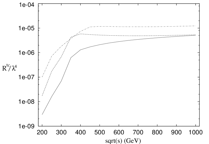
FIG. 2.: $R^{tc}/\lambda^{4}$ vs. $\sqrt{s}$ for case 1 (solid), case 2 (dashed), and case 3 (dot-dashed), with $m_{t}=180$ GeV. See Eq. (27).

As already discussed in Ref. [1], we take $m_{t}\!\simeq\!180$ GeV and vary the masses of the scalar and pseudoscalar fields in a range between 200 GeV and 1 TeV. Larger values of the scalar masses are excluded by the requirement of a weak-coupled scalar sector. The phase $\alpha$ does not play a relevant role and, as we discuss in Appendix B, in our qualitative analysis we will set $\alpha\!=\!0$. In this case, as we can read in Eqs. (6) or (9), $H^{0}\!=\!\bar{H}^{0}+v$, $H^{1}\!=\!h^{0}$, and $H^{2}\!=\!A^{0}$ and the only new contributions come from $h^{0}$ and $A^{0}$. In Fig. 2 we plot $R^{tc}/\lambda^{4}$ as a function of $\sqrt{s}$ for a sample of relevant cases, in which one of the scalar particles is taken to be light ($M_{l}\!\simeq\!200$ GeV) compared to the other two ($M_{h}\!\simeq\!1$ TeV), i.e.

$$1)\,\,\,m_{h} = M_{\ell}\,\,\,\,\,\mbox{and}\,\,\,\,\,m_{A}\simeq m_{c}\simeq M_{h}\,;$$ (27)

$$2)\,\,\,m_{A} = M_{\ell}\,\,\,\,\,\mbox{and}\,\,\,\,\,m_{h}\simeq m_{c}\simeq M_{h}\,;$$ (28)

$$3)\,\,\,m_{c} = M_{\ell}\,\,\,\,\,\mbox{and}\,\,\,\,\,m_{h}\simeq m_{A}\simeq M_{h}\,.$$ (29)

where $m_{h}$ and $m_{A}$ are the neutral scalar and pseudoscalar masses and $m_{c}$ is the charged scalar mass respectively. We find that even with different choices of $m_{h}$, $m_{A}$ and $m_{c}$ it is difficult to push $R^{tc}/\lambda^{4}$ much higher than $10^{-5}$. Therefore the three cases illustrated in Fig. 2 appear to be a good sample to illustrate the type of predictions we can obtain for the rate for top-charm production in model III.

From Fig. 2, we also see that going to energies much larger than $\sim 400$–500 GeV (i.e. $\sim 2M_{l}$) does not gain much in the rate and in this case $R^{tc}/\lambda^{4}$ can be as much as $10^{-5}$. Since it is reasonable to expect $10^{4}$–$10^{5}$ $\mu^{+}\mu^{-}$ events in a year of running for the next generation of $e^{+}e^{-}$ colliders ($\int{\cal L}\simeq 5\times 10^{33}\,\mbox{cm}^{-2}\mbox{sec}^{-1}$) at $\sqrt{s}=500$ GeV, this signal could be at the detectable level only for not too small values of the arbitrary parameter $\lambda$. Thus we can expect experiments to be able to constrain $\lambda\mathrel{\lower 4.0pt\hbox{$\sim$}}\hskip-12.5pt\raise 1.6pt\hbox{$<$}\;1$, for scalar masses of a few hundred GeVs.

IV Rare top decays: $t\rightarrow c\gamma,Z,g$

Starting from the form factors defined in Eq. (17) and given in Appendix B, we can also easily derive the rates for rare top decays like $t\rightarrow c\gamma$, $t\rightarrow cZ$ and $t\rightarrow cg$. The study of rare top decays has been often emphasized in the literature [15, 16, 10, 7], in particular, as a potential source of evidence for new physics. Indeed, as we can read from Table I, these decays are extremely suppressed in the SM and they are quite small even in the 2HDM’s without tree level FCNC’s (i.e. both in model I and in model II) [15, 16]. This is due to a strong GIM suppression from the small value of the internal quark masses $m_{d,s,b}$ as well as the large tree level rate for $t\rightarrow bW$. On the other hand, these rare top decays normally get enhanced in models with FCNC’s and this motivates us to estimate their branching ratio in model III. From the experimental point of view the prospects for the three modes, $t\rightarrow c\gamma$, $cZ$, and $cg$ are quite different. In particular, $t\rightarrow cg$ could be quite problematic for a hadron collider and the backgrounds will have to be considered before one can ensure that they do not represent a serious limitation. On the other hand, for the $e^{+}e^{-}$ case background issues are less likely to be a serious problem even for $t\rightarrow cg$.

Decay	SM	Model I	Model II	Model III
$t\rightarrow c\gamma$	$\sim 5\cdot 10^{-12}$	$10^{-13}\!-\!10^{-11}$	$10^{-13}\!-\!10^{-9}$	$10^{-12}\!-\!10^{-7}$
$t\rightarrow cZ$	$\sim 10^{-13}$	$10^{-13}\!-\!10^{-11}$	$10^{-13}\!-\!10^{-10}$	$10^{-8}\!-\!10^{-6}$
$t\rightarrow cg$	$\sim 5\cdot 10^{-11}$	$10^{-11}\!-\!10^{-9}$	$10^{-11}\!-\!10^{-8}$	$10^{-8}\!-\!10^{-4}$

TABLE I.: Values of $Br(t\rightarrow c\gamma)$, $Br(t\rightarrow cZ)$, and $Br(t\rightarrow cg)$ for $m_{t}\simeq 180$ GeV, in the SM and in the 2HDM’s denoted as Model I, Model II, and Model III. Each range is obtained by varying $m_{c}$, $m_{h}$, $m_{A}$, $\tan\beta,\ldots$ over a broad region of the parameter space of the corresponding model, as explained in the text. For Model III, we have fixed $\lambda_{ij}\simeq\lambda=1$ in the FC couplings.

In model III the modes $t\rightarrow c\gamma$ and $t\rightarrow cZ$ have been previously considered [7] and their rates are given by

$$\Gamma(t\rightarrow c\gamma)=\frac{1}{(16\pi^{2})^{2}}\frac{1}{8\pi}\left(|C^{\gamma}|^{2}+|D^{\gamma}|^{2}\right)$$ (30)

$$\Gamma(t\rightarrow cZ) = \frac{1}{(16\pi^{2})^{2}}\frac{1}{16\pi m_{t}}\left(1-\frac{M_{Z}^{2}}{m_{t}^{2}}\right)\left(\frac{m_{t}^{2}}{M_{Z}^{2}}-1\right)\left[(m_{t}^{2}+2M_{Z}^{2})\left(|A^{Z}|^{2}+|B^{Z}|^{2}\right)\right.$$ (31)

$$- \left.6M_{Z}^{2}{\rm Re}\,(A^{Z*}C^{Z}-B^{Z*}D^{Z})+M_{Z}^{2}\left(\frac{M_{Z}^{2}}{m_{t}^{2}}+2\right)\left(|C^{Z}|^{2}+|D^{Z}|^{2}\right)\right]\,\,\,.$$ (32)

The rate for $t\rightarrow cg$ can be written in an analogous manner, as,

$$\Gamma(t\rightarrow cg)=\frac{1}{(16\pi^{2})^{2}}\frac{1}{8\pi}C_{F}\left(|C^{g}|^{2}+|D^{g}|^{2}\right)$$ (33)

where $C_{F}=(N^{2}-1)/2N$.

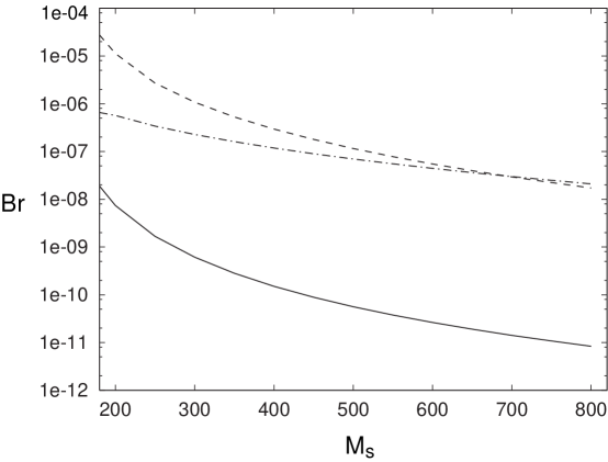
FIG. 3.: Branching fraction for $t\rightarrow c\gamma$ (solid), $t\rightarrow cZ$ (dot-dashed), and $t\rightarrow cg$ (dashed) as a function of a common scalar mass $M_{s}$, when $m_{t}=180$ GeV.

The branching ratios reported in Table I are obtained by normalizing $\Gamma(t\rightarrow c\gamma)$, $\Gamma(t\rightarrow cZ)$ and $\Gamma(t\rightarrow cg)$, for simplicity, just to the main decay $t\rightarrow bW$ rate, i.e.

$$\Gamma(t\rightarrow bW)=\frac{G_{F}}{8\pi\sqrt{2}}|V_{tb}|^{2}m_{t}^{3}\left(1-\frac{M_{W}^{2}}{m_{t}^{2}}\right)\left(1+\frac{M_{W}^{2}}{m_{t}^{2}}-2\frac{M_{W}^{4}}{m_{t}^{4}}\right)\,\,\,.$$ (34)

The branching ratios for model I and model II are deduced from the analysis of Ref. [15, 16], with $m_{t}\!\simeq\!180$ GeV. The results for model III are obtained by varying the neutral and the charged scalar masses between 200 GeV and 1 TeV, assuming different patterns as explained in the preceding section (see for instance Eq. (27)). In particular the upper bounds on the different branching ratios given in Table I are obtained by taking the scalars to have a common and relatively small mass. We also notice that in model III the results show a significant dependence on $m_{t}$, such that the numbers in Table I change on the average by as much as an order of magnitude when $m_{t}$ is varied between 150 GeV and 200 GeV. This sensitivity to $m_{t}$ may become relevant when the experiments ever get to the point of being able to measure this type of rare top decay. Finally, in the FC couplings of Eq. (16) we also take all the $\lambda_{ij}$ parameters to be equal to $\lambda$. In particular, the numbers in Table I are given for $\lambda\!=\!1$.

Our analytical expressions for the form factors contain some differences with respect to Ref. [7], as explained in Appendix B [17]. Numerically they end up being most relevant for $t\rightarrow c\gamma$. Fig. 3 illustrates the case in which a common value $M_{s}$ is taken for all the scalar masses, as might be useful for comparison [18] with Fig. 2 of Ref. [7]. We can see that the analytical difference between us and Ref. [7] translates into a numerical difference of more than one order of magnitude for the $t\rightarrow c\gamma$ decay rate.

From Table I, we see that $Br(t\rightarrow c\gamma)$, $Br(t\rightarrow cZ)$, and $Br(t\rightarrow cg)$ can be substantially enhanced with respect both to the SM and to the 2HDM’s with no FCSC’s (i.e. model I and model II). Depending on the size of the FC couplings, in model III we can gain even more than two of orders of magnitude in each branching ratio. This is likely to make a crucial difference at the next generation of lepton and hadron colliders where a large number of top quarks will be produced. Therefore these machines will be sensitive to signals from non-standard top decays and should be able to put stringent bounds on the new interactions involved, the FC couplings of model III in our case. In view of these future possibilities, a careful study of the FC couplings of the model is mandatory and we will analyze the constraints that emerge from existing experiments in Secs. VI–VII.

V Top-charm production at $\mu^{+}\mu^{-}$ colliders

Another interesting possibility to study top-charm production is offered by muon colliders [2]. Although very much in the notion stage at present, a $\mu^{+}\mu^{-}$ collider has been suggested [19, 20, 21, 22] as a possible lepton collider. Muon colliders are especially interesting for two main reasons. They can allow a detailed study of the $s$-channel Higgs and also they may make it feasible to have high energy lepton colliders in the multi-TeV regime. Neither of these goals is attainable with an $e^{+}e^{-}$ collider.

If muon colliders are eventually shown to be a practical and desirable tool, most of the applications would be very similar to electron colliders. One additional advantage alluded to above, however, is that they may be able to produce Higgs bosons (${\cal H}$) in the $s$-channel in sufficient quantity to study their properties directly [19, 23, 24, 25, 2]. The crucial point is that in spite of the fact that the $\mu^{+}\mu^{-}{\cal H}$ coupling, being proportional to $m_{\mu}$, is very small, if the muon collider is run on the Higgs resonance, $\sqrt{s}=m_{\cal H}$, Higgs bosons may be produced at an appreciable rate [19, 23, 24, 25, 2].

At $\sqrt{s}=m_{\cal H}$, the cross section for producing ${\cal H}$, $\sigma_{\cal H}$, normalized to $\sigma_{0}=\sigma(\mu^{+}\mu^{-}\rightarrow\gamma^{*}\rightarrow e^{+}e^{-})$, is given by [24, 25]

$$R({\cal H})={\sigma_{\cal H}\over\sigma_{0}}={3\over\alpha_{e}^{2}}B_{\mu}^{\cal H}$$ (35)

where $B_{\mu}^{\cal H}$ is the branching ratio of ${\cal H}\rightarrow\mu^{+}\mu^{-}$ and $\alpha_{e}$ is the QED fine structure constant. If the Higgs is very narrow, the exact tuning to the resonance implied in Eq. (35) may not in general be possible. The effective rate of Higgs production will then be given by [25]

$$\tilde{R}({\cal H})=\left[\frac{\Gamma_{\cal H}}{m_{\cal H}\delta}\arctan\frac{m_{\cal H}\delta}{\Gamma_{\cal H}}\right]R({\cal H})$$ (36)

where it is assumed that the energy of the beam has a finite spread described by $\delta$

$$m_{\cal H}^{2}(1-\delta)<s<m_{\cal H}^{2}(1+\delta)$$ (37)

and $s$ is uniform about this range.

In a recent paper [2] we have considered the simple but fascinating possibility that such a Higgs, ${\cal H}$, has a flavor-changing ${\cal H}t\bar{c}$ coupling, as is the case in model III or in any other 2HDM with FCNC’s. The process $\mu^{+}\mu^{-}\rightarrow t\bar{c}+\bar{t}c$ will then arise at the tree level as illustrated in Fig. 4. It will give a signal which should be easy to identify, is likely to take place at an observable rate, and has a negligible SM background. Thus the properties of the important ${\cal H}t\bar{c}$ coupling may be studied in detail.

FIG. 4.: Tree level contributions to $\mu^{+}\mu^{-}\rightarrow\bar{t}c+t\bar{c}$ in model III.

For illustrative purposes we take ${\cal H}=h^{0}$ in model III where $\alpha=0$ (case 1) or $\pi/4$ (case 2). The main distinction between the two cases is that in case 2 the decays $h^{0}\rightarrow ZZ,\ WW$ are possible while in case 1 they are not (see Appendix A for the relevant Feynman rules). Thus case 1 is very similar to ${\cal H}=A^{0}$. This will matter in computing the total width of the $h^{0}$ boson, i.e. the $Br(h^{0}\rightarrow tc)$, while it was completely irrelevant in the $e^{+}e^{-}\rightarrow\gamma^{*},Z^{*}\rightarrow t\bar{c}+c\bar{t}$ calculation.

In general the FC coupling of $h^{0}$ to $t\bar{c}$ can be written as

$$C_{htc}=\frac{1}{\sqrt{2}}\left(\xi_{tc}P_{R}+\xi_{ct}^{\dagger}P_{L}\right)\cos\alpha\equiv\frac{g\sqrt{m_{t}m_{c}}}{2m_{W}}(\chi_{R}P_{R}+\chi_{L}P_{L})$$ (38)

where $\chi_{L}$ and $\chi_{R}$ are in general complex numbers and of order unity if Eq. (16) applies. In particular we will consider the case in which $\lambda_{ct}=\lambda\simeq O(1)$ (see Eq. (16)) and $\chi_{L}$ and $\chi_{R}$ are real. We treated the more general case in Ref. [2] to which we refer for further details.

The decay rate to $t\bar{c}$ is thus

$$\Gamma({\cal H}\rightarrow t\bar{c})={3g^{2}m_{t}m_{c}m_{\cal H}\over 32\pi M_{W}^{2}}\left[{(m_{\cal H}^{2}-m_{t}^{2})^{2}\over m_{\cal H}^{4}}\right]\left({|\chi_{R}|^{2}+|\chi_{L}|^{2}\over 2}\right)$$ (39)

and, $\Gamma({\cal H}\rightarrow t\bar{c})=\Gamma({\cal H}\rightarrow c\bar{t})$ at the tree level that we are considering for now.

As we did in Sec. III for the $e^{+}e^{-}$ case, also in the $\mu^{+}\mu^{-}$ case we can define the analogue of $R^{tc}$ in Eq. (26) to be

$$R_{tc}=\tilde{R}({\cal H})\,(B^{\cal H}_{t\bar{c}}+B^{\cal H}_{c\bar{t}})$$ (40)

where $B^{\cal H}_{t\bar{c}}$ and $B^{\cal H}_{c\bar{t}}$ are the branching ratio for ${\cal H}\rightarrow t\bar{c}$ and ${\cal H}\rightarrow c\bar{t}$ respectively. We estimate $R_{tc}$ in the following two cases:

1. case 1: $\alpha=0$ ;

2. case 2: $\alpha=\pi/4\,\,.$

FIG. 5.: $R_{tc}$ for $\delta=0$, $10^{-3}$ and $10^{-2}$ in case 1 (set of solid curves) and case 2 (set of dashed curves). We also plot $\tilde{R}({\cal H})$ in case 1 (dot-dashed) and case 2 (dotted).

Using the result in Eq. (39) [2] and taking the expressions for the standard partial widths for ${\cal H}$ (e.g. $\Gamma({\cal H}\rightarrow t\bar{t})$, $\Gamma({\cal H}\rightarrow b\bar{b}),\ldots$) from the literature [11], we obtain the following results. In case 1, if $m_{\cal H}$ is below the $t\bar{t}$ threshold, $R_{tc}$ is about $10^{-2}-1$ and in fact $tc$ makes up a large branching ratio. Above the $t\bar{t}$ threshold $R_{tc}$ drops. For case 2 the branching ratio is smaller due to the $WW$ and $ZZ$ threshold at about the same mass as the $tc$ threshold and so $R_{tc}$ is around $10^{-3}$. All these results are illustrated in Fig. 5, where we plot $\tilde{R}({\cal H})$ and $R_{tc}$ with $\delta=0$, $10^{-3}$ and $10^{-2}$ in case 1 and case 2 .

For a specific example, let us take $m_{\cal H}=300$ GeV, i.e. $\sigma_{0}\approx 1$ pb. For a luminosity of $10^{34}\mbox{cm}^{-2}\mbox{s}^{-1}$, a year of $10^{7}$ s ($1/3$ efficiency) and for $\delta=10^{-2}$, case 1 will produce about $5\times 10^{3}(t\bar{c}+\bar{t}c)$ events and case 2 will produce about $150$ events. Given the distinctive nature of the final state and the lack of a SM background, sufficient luminosity should allow the observation of such events.

If such events are observed, the $\mu^{+}\mu^{-}$ collider offers the additional interesting possibility of extracting the values of the $\chi_{L}$ and $\chi_{R}$ couplings in Eq. (38) separately. What is measured initially at a $\mu^{+}\mu^{-}$ collider is $R_{tc}$. One is required to know the total width of the ${\cal H}$ and the energy spread of the beam in order to translate this into $\Gamma({\cal H}\rightarrow t\bar{c})$. This then allows the determination of $|\chi_{L}|^{2}+|\chi_{R}|^{2}$ (see Eq. (39)). To get information separately on the two couplings we note that the total helicity of the top quark is

$${\bf H}_{t}=-{\bf H}_{\bar{t}}={|\chi_{R}|^{2}-|\chi_{L}|^{2}\over|\chi_{R}|^{2}+|\chi_{L}|^{2}}$$ (41)

from which one may therefore infer $|\chi_{L}|$ and $|\chi_{R}|$. Of course the helicity of the $t$ cannot be observed directly. However, following the discussion of [25, 2] one may obtain it from the decay distributions of the top quark. Unfortunately in the limit of small $m_{c}$ the helicity of the $c$-quark is conserved. Hence the relative phase of $\chi_{L}$ and $\chi_{R}$ may not be determined since the two couplings do not interfere.

VI Constraints from $F^{0}\!\!-\!\!\bar{F}^{0}$ mixing processes

From the previous analysis we see that both $e^{+}e^{-}\,,\,\mu^{+}\mu^{-}\rightarrow\bar{c}t+\bar{t}c$ and $t\rightarrow c\gamma,Z,g$ could be of some experimental relevance depending on the size of the FC couplings of model III. As is well known from the literature on FCNC’s, the most dangerous constraints on tree level FC couplings come usually from $F^{0}\!-\!\bar{F}^{0}$ mixing processes ($F=K,B_{d},D$) [3, 4, 5]. In these references we can find the bounds imposed on some tree level FC couplings by different $F^{0}\!-\!\bar{F}^{0}$ mixing processes. Due to the specific structure of the couplings of model III and to the new phenomenology at hand, we think that a more careful analysis is due, which takes into account both tree level and loop contributions. We have examined the $\Delta F\!=\!2$ mixing processes in detail and concluded that both the $K^{0}\!-\!\bar{K}^{0}$ and the $B^{0}_{d}\!-\!\bar{B}^{0}_{d}$ mixings are particularly effective in constraining some FC couplings, while the experimental determination of the $D^{0}\!-\!\bar{D}^{0}$ mixing is, for now, not good enough to compete with the other two mixings. However, due to the different flavor structure of the $D^{0}\!-\!\bar{D}^{0}$ mixing, it would be extremely important to have a good experimental determination in this case as well. We will address the problem more specifically later on in this section.

In a model with FCNC’s, $F^{0}\!-\!\bar{F}^{0}$ mixing processes can arise at the tree level. Therefore they are likely to be greatly enhanced with respect to the SM where they appear only at the one loop level. Due to the good agreement between the SM prediction and the experimental determination of the mass difference in the $K^{0}\!-\!\bar{K}^{0}$ and $B^{0}_{d}\!-\!\bar{B}^{0}_{d}$ systems, any tree level contribution from elementary FC couplings needs to be strongly suppressed. This was the original motivation for imposing on the 2HDM’s a discrete symmetry [9] which could prevent tree level FCNC’s from appearing (model I and model II). Our goal will be now to verify if, in model III, the hierarchy imposed on the $\xi_{ij}^{U,D}$ couplings by the ansatz in Eq. (16) is strong enough to make the tree level contribution to any $F^{0}\!-\!\bar{F}^{0}$ mixing sufficiently small to be compatible with the experimental constraints.

For any $F^{0}\!-\!\bar{F}^{0}$ mixing we have evaluated, both at the tree level and at the one loop level, the mass difference between the mass eigenstates of the system, given respectively by

$$M_{K}\Delta M_{K} \simeq \mbox{Re}\langle K^{0}|(\bar{s}d)_{V-A}(\bar{s}d)_{V-A}|\bar{K}^{0}\rangle$$ (42)

$$M_{B_{d}}\Delta M_{B_{d}} \simeq |\langle B^{0}_{d}|(\bar{b}d)_{V-A}(\bar{b}d)_{V-A}|\bar{B}^{0}_{d}\rangle|$$ (43)

$$M_{D}\Delta M_{D} \simeq |\langle D^{0}|(\bar{c}u)_{V-A}(\bar{c}u)_{V-A}|\bar{D}^{0}\rangle|$$ (44)

where we use the notation $(\bar{q}q^{\prime})_{V-A}=\bar{q}\gamma^{\mu}(1-\gamma^{5})q^{\prime}$. The tree level contributions for each different mixing are shown in Fig. 6, while a sample of one loop contributions are illustrated in Figs. 7 and 8, for the box and the penguin diagrams respectively.

FIG. 6.: Tree level contributions to each different $F^{0}\!-\!\bar{F}^{0}$ mixing, for $F=K,B_{d},D$, in model III.

FIG. 7.: Box diagrams which contribute at one loop to the $K^{0}\!-\!\bar{K}^{0}$ and to the $B^{0}_{d}\!-\!\bar{B}_{d}^{0}$ mixing, in model III. The $D^{0}\!-\!\bar{D}^{0}$ case is obtained by appropriately replacing the external and internal quark states.

FIG. 8.: Penguin diagrams which contribute at one loop to the $K^{0}\!-\!\bar{K}^{0}$ and to the $B^{0}_{d}\!-\!\bar{B}_{d}^{0}$ mixing, in model III. The $D^{0}\!-\!\bar{D}^{0}$ case is obtained by appropriately replacing the external and internal quark states.

In our analysis we have made some general approximations which we want to discuss first.

1. We observe that, as in the calculation of the $Ztc$ and $\gamma tc$ form factors in Sec. III, also in this case the value of the phase $\alpha$ plays a minor role numerically. Therefore, as we did in Sec. III, we will set $\alpha\!=\!0$ in the following analysis. Once that is done we can focus our attention only on the contributions coming from $H^{1}\!=\!h^{0}$, $H^{2}\!=\!A^{0}$, and $H^{+}$. The possibility of having FCNC’s induced by $h^{0}$ and $A^{0}$ will give rise to the tree level $\Delta F\!=\!2$ mixings of Fig. 6.

2. In the evaluation of the one loop contributions to the $\Delta F\!=\!2$ mixings, we will take advantage of the fact that they are due to scalar bosons whose couplings to the quark fields are proportional to the masses of the quarks involved and, for the charged scalar, to some combinations of CKM matrix elements. Therefore, in each case we will consider only the dominant contribution, which quite often will correspond to the diagrams with a heavy quark loop. This procedure is clearly more approximate than the exact calculation one uses to perform in the SM [26], but a similar order of accuracy would not be necessary in our case. Nevertheless, as a check of our calculation, we have reproduced the SM result for each mixing and used it as a reference point to fix the right relative signs and normalizations.

3. The $\Delta F\!=\!2$ effective interactions generated by the new scalar fields are often more complicated compared to the SM results [26], because the scalar-fermion couplings involve more chiral structures. Therefore, the evaluation of the mass difference in the various $F^{0}\!-\!\bar{F}^{0}$ systems will involve the matrix elements of operators other than just the SM one

   $$O^{SM}_{\Delta F\!=\!2}=O^{F}_{VLL}=(\bar{f}\gamma^{\mu}(1-\gamma_{5})q)(\bar{f}\gamma_{\mu}(1-\gamma_{5})q)\,\,.$$ (45)

   In general, matrix elements of the following operators are involved

   $$O_{S}^{F} = (\bar{f}q)(\bar{f}q)$$ (46)

   $$O_{P}^{F} = (\bar{f}\gamma_{5}q)(\bar{f}\gamma_{5}q)$$ (47)

   $$O_{V}^{F} = (\bar{f}\gamma^{\mu}q)(\bar{f}\gamma_{\mu}q)$$ (48)

   $$O_{A}^{F} = (\bar{f}\gamma^{\mu}\gamma_{5}q)(\bar{f}\gamma_{\mu}\gamma_{5}q)$$ (49)

   $$O_{VLR}^{F} = (\bar{f}\gamma^{\mu}(1-\gamma_{5})q)(\bar{f}\gamma_{\mu}(1+\gamma_{5})q)$$ (50)

   $$O_{LL}^{F} = (\bar{f}(1-\gamma_{5})q)(\bar{f}(1-\gamma_{5})q)$$ (51)

   $$O_{LR}^{F} = (\bar{f}(1-\gamma_{5})q)(\bar{f}(1+\gamma_{5})q)$$ (52)

   for $F=K,B_{d},D$; $f=s,b,c$ and $q=d,u$ depending on the $F^{0}$ meson that we consider. The matrix element of $O^{SM}_{\Delta F\!=\!2}$ is usually given as

   $$\langle F^{0}|O^{SM}_{\Delta F\!=\!2}|\bar{F}^{0}\rangle=B_{F}\langle F^{0}|O^{SM}_{\Delta F\!=\!2}|\bar{F}^{0}\rangle_{VIA}$$ (53)

   where the ratio of the matrix element itself to its value in the Vacuum Insertion Approximation (VIA) is expressed by the $B$-parameter $B_{F}$. Extensive non-perturbative studies of $B_{K}$ and $B_{B}$ exist in the literature, especially from lattice calculations [27]. For our purpose, we just want to evaluate each matrix element in the VIA and use a common $B$-parameter (the one for $O^{F}_{VLL}$). Clearly this is only an approximation. Such an approximation may be problematic in the SM, where one aims to get a very precise prediction, but it suffices for our qualitative discussion. In particular, we will assume $B_{K}\!=\!0.75$, $B_{B}\!=\!1$, and $B_{D}\!=\!1$ [27]. Moreover, according to Ref. [28] and to analogous calculations we performed for those operators that were not considered there, we will use the following expressions for the $\Delta F\!=\!2$ matrix elements of the $O_{a}^{F}$ operators (for $a=S,P,V,A,VLL,VLR,LL,LR$) in the VIA

   $$M_{S}^{F} = \langle F^{0}|O^{F}_{S}|\bar{F}^{0}\rangle_{\scriptscriptstyle VIA}=-\frac{1}{6}M^{0,F}_{P}+\frac{1}{6}M^{0,F}_{A}$$ (54)

   $$M_{P}^{F} = \langle F^{0}|O^{F}_{P}|\bar{F}^{0}\rangle_{\scriptscriptstyle VIA}=\frac{11}{6}M^{0,F}_{P}-\frac{1}{6}M^{0,F}_{A}$$ (55)

   $$M_{V}^{F} = \langle F^{0}|O^{F}_{V}|\bar{F}^{0}\rangle_{\scriptscriptstyle VIA}=\frac{2}{3}M^{0,F}_{P}+\frac{1}{3}M^{0,F}_{A}$$ (56)

   $$M_{A}^{F} = \langle F^{0}|O^{F}_{A}|\bar{F}^{0}\rangle_{\scriptscriptstyle VIA}=-\frac{2}{3}M^{0,F}_{P}+\frac{7}{3}M^{0,F}_{A}$$ (57)

   $$M_{VLL}^{F} = \langle F^{0}|O^{F}_{VLL}|\bar{F}^{0}\rangle_{\scriptscriptstyle VIA}=\frac{8}{3}M^{0,F}_{A}$$ (58)

   $$M_{VLR}^{F} = \langle F^{0}|O^{F}_{VLR}|\bar{F}^{0}\rangle_{\scriptscriptstyle VIA}=\frac{4}{3}M^{0,F}_{P}-2M^{0,F}_{A}$$ (59)

   $$M_{LL}^{F} = \langle F^{0}|O^{F}_{LL}|\bar{F}^{0}\rangle_{\scriptscriptstyle VIA}=\frac{5}{3}M^{0,F}_{P}$$ (60)

   $$M_{LR}^{F} = \langle F^{0}|O^{F}_{LR}|\bar{F}^{0}\rangle_{\scriptscriptstyle VIA}=-2M^{0,F}_{P}+\frac{1}{3}M^{0,F}_{A}$$ (61)

   for $F=K,B_{d},D$. All the previous matrix elements have been expressed in terms of the matrix elements of the only two operators which do not vanish on the vacuum, i.e.

   $$M^{0,F}_{P} = \langle\bar{F}^{0}|\bar{\psi}_{f}\gamma_{5}\psi_{q}|0\rangle\langle 0|\bar{\psi}_{f}\gamma_{5}\psi_{q}|F^{0}\rangle=-f_{F}^{2}\frac{M_{F}^{4}}{(m_{f}+m_{q})^{2}}$$ (62)

   $$M^{0,F}_{A} = \langle\bar{F}^{0}|\bar{\psi}_{f}\gamma_{\mu}\gamma_{5}\psi_{q}|0\rangle\langle 0|\bar{\psi}_{f}\gamma^{\mu}\gamma_{5}\psi_{q}|F^{0}\rangle=f_{F}^{2}M_{F}^{2}$$ (63)

   where $M_{F}$ and $m_{f}$ indicate respectively the mass of the meson and of the quark of flavor $f$. The recent evaluation of the pseudoscalar decay constants $(f_{F})$ can be found in the literature [29]. In our calculation we have used the following set of values: $f_{K}=0.160$ GeV, $f_{B}=0.175$ GeV, and $f_{D}=0.200$ GeV, where the first value comes from experiments and the last two are representatives of lattice calculations.

4. No QCD corrections have been taken into account for model III. From the SM case [30, 31] we know that these corrections can be important when a precise comparison with the experimental data is needed [32]. However, in model III they would affect the evaluation of the constraints at a much higher degree of accuracy compared to the approximations that we are adopting; therefore we neglect them.

We now proceed to the discussion of the important results. In Eq. (16) we basically parametrize our ignorance of the FC couplings of model III introducing the $\lambda_{ij}^{U,D}$ mixing parameters. Therefore, the constraints we are going to impose will allow us to deduce the order of magnitude of some of the $\lambda_{ij}^{U,D}$. Due to the fact that the analysis of any $F^{0}\!-\!\bar{F}^{0}$ mixing will involve both tree level and one loop contributions, we will have to deal with several couplings at the same time. In order to simplify the analysis we will first take all the $\lambda_{ij}^{U,D}$ parameters to be equal. Depending on the result of this first approach to the problem, we will consider the possibility that different couplings are differently enhanced or suppressed. According to this logic, we have considered the following cases, corresponding to three possible assumptions on the FC couplings of Eq. (16).

  Case 1

: $\lambda_{ij}\simeq\lambda$ common to all the FC couplings.

  Case 2

: $\lambda_{ui},\lambda_{dj}\ll 1$ for $i,j=1,2,3$, i.e. negligible FC couplings for the first generation and no assumptions on the other FC couplings.

  Case 3

: as Case 2 but with the further assumption that

$$\lambda_{bb},\lambda_{sb}\gg 1\,\,\,\,\mbox{and}\,\,\,\,\lambda_{tt},\lambda_{ct}\ll 1\,\,.$$ (64)

The results for each $F^{0}\!-\!\bar{F}^{0}$ mixing ($F=K,B_{d},D$) in case 1, case 2, and case 3 are reported in Table II, where we also give the corresponding experimental results [33, 34] and the SM predictions [31, 30, 35]. Both for the SM and for each case of model III we also specify whether the dominant contribution is due to tree level or to one loop diagrams. The different relevance of the tree level and one loop contributions and how this imposes constraints on some particular couplings will be explained as we go along the discussion in this section. Moreover, for each different choice of the couplings, we have varied $m_{h}$, $m_{A}$, and $m_{c}$ in the range between 100 GeV and 1 TeV. This is the reason for the range of values that are given in Table II for each case and for each mixing in model III. In this section we will discuss in particular case 1 and case 2. The scenario described by case 3 results from the constraints imposed by $R_{b}$, $\rho$ and $Br(B\rightarrow X_{s}\gamma)$ and will be discussed in some detail in Sec. VI. For convenience, a summary of its results is reported in Table II as well.

In Case 1, i.e. when all the FC couplings are parametrized in terms of a unique $\lambda$, the leading contribution comes from the tree level diagrams of Fig. 6. The one loop contributions are always subleading all over the mass parameter space. For each $F^{0}\!-\!\bar{F}^{0}$ mixing, there are two possible tree level contributions, mediated by an $h^{0}$ and an $A^{0}$ neutral field respectively. We want to consider them separately because in our analysis we will vary $m_{h}$ and $m_{A}$ independently. Moreover the two contributions differ by the chiral structure of the resulting four fermion effective interaction, of $S$-type for the $h^{0}$ exchange and of $P$-type for the $A^{0}$ exchange (see their Feynman rules in Appendix A). Since $M^{F}_{P}\gg M^{F}_{S}$, the distinction between the two tree level contributions becomes important and we write them as follows

		$K^{0}\!-\!\bar{K}^{0}$	$B^{0}_{d}\!-\!\bar{B}^{0}_{d}$	$D^{0}\!-\!\bar{D}^{0}$
Experiment		$3.51\cdot 10^{-15}$	$3.26\cdot 10^{-13}$	$<1.32\cdot 10^{-13}$
SM	One Loop	$1.4-4.6\cdot 10^{-15}$	$10^{-13}-10^{-12}$	$10^{-17}-10^{-16}$
Model III (Case 1)	Tree Level	$10^{-14}-10^{-13}$	$10^{-12}-10^{-11}$	$10^{-13}-10^{-12}$
Model III (Case 2)	One Loop	$10^{-18}-10^{-17}$	$10^{-14}-10^{-13}$	$10^{-17}-10^{-18}$
Model III (Case 3)	One Loop	$10^{-20}-10^{-19}$	$10^{-17}-10^{-16}$	$10^{-14}-10^{-15}$

TABLE II.: Experimental values and theoretical predictions in the SM and in model III for $\Delta M_{F}$ (in GeV) for different $F^{0}-\bar{F}^{0}$ mixings ($F=K,B_{d},D$). Case 1, case 2, and case 3 correspond to three possible scenarios in which different assumptions are made on the FC couplings, as described in the text. Each range is obtained by varying the parameters of the model over a large region of the parameter space, compatible with phenomenology and with the assumption of weakly coupled scalar fields. The leading contributions (tree level or one loop) are also indicated in each case.

$$h^{0} \rightarrow \Delta M_{F}^{\scriptscriptstyle tree}=2\left(\xi^{U,D}_{fq}\right)^{2}\frac{1}{m_{h}^{2}}M_{S}^{F}$$ (65)

$$A^{0} \rightarrow \Delta M_{F}^{\scriptscriptstyle tree}=-2\left(\xi^{U,D}_{fq}\right)^{2}\frac{1}{m_{A}^{2}}M_{P}^{F}$$ (66)

for $F=K,B,D$, $f=s,b,c$, and $q=d$ or $u$ depending on the mixing that is of interest. In particular, since $M^{F}_{P}\gg M^{F}_{S}$, we observe that an interesting possibility will be to have a light $h^{0}$ and a much heavier $A^{0}$. In this way the $A^{0}$ contribution would not be too large, while we would still have a light scalar field with FC interactions.

FIG. 9.: Upper bounds on $\lambda$ imposed by the tree level mixings illustrated in Fig. 6: $K^{0}\!-\!\bar{K}^{0}$ (dashed), $B^{0}_{d}\!-\!\bar{B}^{0}_{d}$ (solid), and $D^{0}\!-\!\bar{D}^{0}$ (dot-dashed).

In Fig. 9 we illustrate the constraints imposed on the parameter $\lambda$ by the tree level mixings in the $K^{0}\!-\!\bar{K}^{0}$, $B^{0}_{d}\!-\!\bar{B}^{0}_{d}$, and $D^{0}\!-\!\bar{D}^{0}$ case respectively. We recall that $\lambda$ is common to the three FC couplings which govern the tree level mixings

$$\xi^{D}_{sd}=\lambda\frac{\sqrt{m_{s}m_{d}}}{v}\,\,\,,\,\,\,\xi^{D}_{bd}=\lambda\frac{\sqrt{m_{b}m_{d}}}{v}\,\,\,,\,\,\,\xi^{U}_{cu}=\lambda\frac{\sqrt{m_{c}m_{u}}}{v}$$ (67)

The three curves represent the upper bounds on $\lambda$ imposed by the present experimental results (see Table II) for different values of the neutral pseudoscalar mass $m_{A}$, when we fix $m_{h}=200$ GeV. Lighter values of $m_{h}$ would not give any relevant change to these bounds. Therefore, for each value of $m_{A}$, the region above a given curve is ruled out by the corresponding $F^{0}\!-\!\bar{F}^{0}$ mixing. As we can see, the most relevant role is played by $K^{0}\!-\!\bar{K}^{0}$ and $B^{0}_{d}\!-\!\bar{B}^{0}_{d}$, which constrain $\lambda$ to be definitely smaller than unity, even for large values of $m_{A}$ (i.e. $m_{A}\sim$ 1 TeV). We have verified that if the experimental precision on $D^{0}\!-\!\bar{D}^{0}$ were increased by one order of magnitude, this mixing would also start to play approximately the same role as $K^{0}\!-\!\bar{K}^{0}$ and $B^{0}_{d}\!-\!\bar{B}^{0}_{d}$, so that the three lines in Fig. 9 would then roughly collapse into one line. We thus see that the $\Delta F\!=\!2$ mixings put severe bounds on the magnitude of the $\xi^{U,D}_{ij}$ couplings when we require all of them to be proportional to a common $\lambda$. For $\lambda\leq 0.1$ (as in Fig. 9 for $m_{A}\sim 200$ GeV) it becomes difficult for the FC couplings of model III to play a role in any process. For instance, the case of top-charm production that we discussed in Sec. III as well as any rare top decay would be too suppressed to be of experimental relevance. On the other hand there is no good reason to assume that all the $\lambda_{ij}$ of Eq. (16) are equal.

Therefore, let us consider next the more general case in which the $\lambda_{ij}$ parameters are different for each different coupling. This is indeed the scenario that we identified as Case 2. We do not have enough specific measurements to constrain all of them independently. However we can make some general remarks. We first observe that the tree level mixings constrain only three couplings to be necessarily small: $\xi_{sd}^{D}$, $\xi_{bd}^{D}$ and $\xi_{uc}^{U}$. In particular, we can take the point of view that the bounds on $\lambda$ in Fig. 9 do apply only to $\lambda_{sd}$, $\lambda_{bd}$, and $\lambda_{uc}$. In general, we can assume that all the FC couplings involving the first family, including also $\xi^{U}_{ut}$, are suppressed. In case 2, the tree level mixings are suppressed enough that some loop contributions might become important. We will consider a loop contribution to become important when it is clearly bigger than the corresponding SM prediction, because only in this case it becomes possible to deduce a strong bound on the new FC couplings.

The one loop diagrams that are most likely to be relevant are those which involve charged scalars only, because the charged couplings can also contain terms that do not involve any of the suppressed couplings (see Eq. (15)) of the first-family. This is not the case for the penguin-like diagrams of Fig. 8, which indeed turn out to be negligible, except for very light and unrealistic values of the neutral scalar and pseudoscalar masses. We mainly have to focus on the box diagrams of Fig. 7 with charged scalars. Moreover, we notice that, if of comparable size, the most relevant box diagrams are going to be those with only one (rather than two) charged scalar boson because they are proportional to the product of two $\lambda_{ij}$ instead of four $\lambda_{ij}$. Thus, if quantitatively relevant with respect to the corresponding SM contributions, they may be as effective as the tree level mixing in constraining the $\lambda$’s.

For the $B^{0}_{d}\!-\!\bar{B}^{0}_{d}$ mixing, the only sizable contribution comes from the diagrams with a top quark in the loop, because the scalar field couples to the quarks as given by Eq. (16), i.e. proportionally to their masses. For $K^{0}\!-\!\bar{K}^{0}$ mixing, the diagram with a charm quark in the loop can be even more important than the one with a top quark, because of the CKM couplings involved. Finally, in the $D^{0}\!-\!\bar{D}^{0}$ case, the most relevant loop contributions come from the box diagram with a bottom quark in the loop. For very light $m_{h}$ and $m_{A}$, the penguin diagrams generated by $h^{0}$ and $A^{0}$, with a top loop, can be comparable.

The results of this analysis can be read off Table II. In spite of the high degree of arbitrariness that we have in model III, we do not find any region of the parameter space in which the one loop contributions in case 2 are definitely larger than the SM prediction. In other words, once the first family is assumed to decouple, the $\Delta F\!=\!2$ processes for $K^{0}\!-\!\bar{K}^{0}$, $B_{d}^{0}\!-\!\bar{B}_{d}^{0}$ and $D^{0}\!-\!\bar{D}^{0}$ place no further constraints on the remaining FC couplings (i.e. $\xi^{U}_{ct}$ and $\xi^{D}_{sb}$). Therefore this analysis tells us that case 2 is compatible with the existing experimental measurements of the $\Delta F\!=\!2$ mixings as long as the second and third generation FC couplings of model III do not have a $\lambda_{ij}$ much larger than 1. This is an interesting result as far as our predictions for $\sigma(e^{+}e^{-}\rightarrow\bar{t}c+\bar{c}t)$ are concerned. Due to the constraints we cannot enhance this cross section in any substantial fashion, but at least it is not suppressed and the values shown in Fig. 2 are roughly correct, with some room for a small enhancement. Similar considerations apply to the case of the rare top decays that we discussed in Sec. IV.

Other more complicated assumptions on the FC couplings of the second and third generation could also be investigated. In order to consider only those possibilities that respect the best fit of the available phenomenological constraints, we will postpone the analysis of other scenarios after the discussion of additional constraints from $Br(B\rightarrow X_{s}\gamma)$, the $\rho$ parameter, and $R_{b}$, in Sec. VII. As we have anticipated in presenting the results of Table II, we will discuss in particular another scenario, the one we have denoted as Case 3, which could be of some physical relevance.

VII $Br(B\rightarrow X_{s}\gamma)$, $\Delta\rho$, $R_{b}$ and the constrained physical model

As it is the case for 2HDM’s without FCNC’s (model I and model II) [36], so also in model III it is very difficult to reconcile the measured value of the inclusive branching fraction for $B\rightarrow X_{s}\gamma$ [37]

$$Br(B\rightarrow X_{s}\gamma)=(2.32\pm 0.51\pm 0.29\pm 0.32)\times 10^{-4}$$ (68)

with the experimental results for $R_{b}$, the ratio of the rate for $Z\rightarrow b\bar{b}$ to the rate for $Z\rightarrow$hadrons. The present situation [38] is such that $R_{b}^{\rm expt}>R_{b}^{\rm SM}$ ($\sim 3\sigma$) [39]

$$R_{b}^{\rm expt}=0.2202\pm 0.0016\,\,\,\,\,,\,\,\,\,\,\,R_{b}^{\rm SM}=0.2156$$ (69)

and the value of $R_{b}^{\rm expt}$ seems to challenge many extensions of the SM [40, 41]. However, several issues on the measurement of this observable are still unclear and require further scrutiny [41, 42]. It is plausible that the experimental situation will change in the future. Therefore we may want to consider both the case in which the constraint from $R_{b}^{\rm expt}$ is enforced and the case in which it is disregarded. A third crucial electroweak (EW) observable in this analysis is given by the $\rho$ parameter, which turns out to be very sensitive to the choice of the mass parameters of any new physics beyond the SM. In a recent paper [41] we have studied the problem in detail, considering two major scenarios in which the constraint from $R_{b}$ is either enforced or disregarded. In the following we will summarize the main results of Ref. [41] and discuss them in the context of the more general picture of model III that we have been tracing till here.

Let us first recall how the presence of an extended scalar sector and of the new FC couplings affects the theoretical prediction for $B(B\rightarrow X_{s}\gamma)$, $\Delta\rho$ and $R_{b}$.

The SM result for the inclusive branching ratio $Br(B\rightarrow X_{s}\gamma)$ [43, 44] can be modified in order to include the contributions from the new scalar fields and we obtain that in model III

$$R=\frac{Br(B\rightarrow X_{s}\gamma)}{Br(B\rightarrow X_{c}e\bar{v}_{e})}\sim\frac{\Gamma(b\rightarrow s\gamma)}{\Gamma(b\rightarrow ce\bar{\nu}_{e})}=\frac{6\alpha}{\pi\,f(m_{c}/m_{b})}\,F\,\left(|C_{7}^{(R)}(m_{b})|^{2}+|C_{7}^{(L)}(m_{b})|^{2}\right)$$ (70)

where $f(m_{c}/m_{b})$ is the phase-space factor for the semileptonic decay and $F$ takes into account some $O(\alpha_{s})$ corrections to both $B\rightarrow X_{c}e\bar{\nu}_{e}$ and $B\rightarrow X_{s}\gamma$ decays (see refs. [41, 45] for further comments). $C_{7}^{(R)}(m_{b})$ and $C_{7}^{(L)}(m_{b})$ are the Wilson coefficients of the two magnetic type operators that occur in model III, for arbitrary $\xi^{U,D}_{ij}$ couplings (see Ref. [41]),

$$Q_{7}^{(R,L)}=\frac{e}{8\pi^{2}}m_{b}\bar{s}\sigma^{\mu\nu}(1\pm\gamma_{5})bF_{\mu\nu}$$ (71)

in the $\Delta S\!=\!1$ effective hamiltonian evaluated at the scale $\mu=m_{b}$. The approximate calculation of $C_{7}^{R}(m_{b})$ and $C_{7}^{L}(m_{b})$ shows that in model III the $Br(B\rightarrow X_{s}\gamma)$ is always larger than the SM one [41]. This feature is very general and the enhancement of the $Br(B\rightarrow X_{s}\gamma)$ depends on the assumptions we make on the new FC couplings and on the masses of the neutral and charged scalar fields.

From the analysis of Ref. [41] it is clear that the $Br(B\rightarrow X_{s}\gamma)$ is very sensitive to any enhancement of the FC couplings. The neutral scalar and pseudoscalar contributions, involving truly new kind of diagrams with respect not only to the SM case but also to model I and model II 2HDM’s, are proportional to $\xi^{D}_{bb}$ and $\xi^{D}_{sb}$. The charged scalar contribution depends on the charged couplings $\xi^{U}_{u_{i}d_{j}}$ and $\xi^{D}_{u_{i}d_{j}}$ for $u_{i}=c,t$ and $d_{j}=s,b$ [46]. In particular, the really leading contribution arises from the diagram with a top quark in the loop and the relevant couplings will then be: $\xi^{U,D}_{ts}$ and $\xi^{U,D}_{tb}$. According to Eq. (15) they are explicitly given by

$$\xi^{U}_{ts} = \xi^{U}_{tt}V_{ts}+\xi^{U}_{tc}V_{cs}\,\,\,\,\,\,,\,\,\,\,\,\,\xi^{U}_{tb}=\xi^{U}_{tt}V_{tb}+\xi^{U}_{tc}V_{cb}$$ (72)

$$\xi^{D}_{ts} = \xi^{D}_{ss}V_{ts}+\xi^{D}_{sb}V_{tb}\,\,\,\,\,\,,\,\,\,\,\,\,\xi^{D}_{tb}=\xi^{D}_{sb}V_{ts}+\xi^{D}_{bb}V_{tb}\,\,\,.$$ (73)

Therefore the final prediction for the $Br(B\rightarrow X_{s}\gamma)$ will depend on the whole set of FC couplings which involve the second and the third generation. A strong enhancement of any of the $\lambda_{ij}$ would conflict with the experimental prediction in Eq. (68), unless some very specific assumptions on the other parameters (couplings and masses) are made [47].

Let us now consider $R_{b}$, defined as

$$R_{b}\equiv\frac{\Gamma(Z\rightarrow b\bar{b})}{\Gamma(Z\rightarrow\hbox{hadrons})}\,\,\,.$$ (74)

Neglecting all finite quark mass effects ($m_{q}\sim 0$) [48], the generic expression for $\Gamma(Z\rightarrow q\bar{q})$, for $q=b,\,c,\ldots$, can be written as

$$\Gamma(Z\rightarrow q\bar{q})=\frac{N_{c}}{6}\frac{\alpha_{e}}{s_{\scriptscriptstyle W}^{2}c_{\scriptscriptstyle W}^{2}}M_{Z}\left[(\Delta_{q,L})^{2}+(\Delta_{q,R})^{2}\right]$$ (75)

where $\alpha_{e}$ is the QED fine structure constant, $N_{c}$ the number of colors, $s_{\scriptscriptstyle W}$ the Weinberg angle and $\Delta_{q,L(R)}$ the chiral left and right couplings of the $Zq\bar{q}$ vertex. They can be written as the sum of a SM piece plus a correction induced, in our case, by the new FC scalar couplings of model III

$$\Delta_{q,L(R)}\equiv\Delta_{q,L(R)}^{\scriptscriptstyle{\rm SM}}+\Delta_{q,L(R)}^{\scriptscriptstyle{\rm NEW}}\,\,\,.$$ (76)

Since $R_{b}$ is in the form of a ratio between two hadronic widths, most EW oblique and QCD corrections cancel, in the massless limit, between the numerator and the denominator. The remaining ones, are absorbed in the definition of the renormalized couplings $\hat{\alpha}$ and ${\hat{s}}_{\scriptscriptstyle W}$ (${\hat{c}}_{\scriptscriptstyle W}$), up to terms of higher order in the electroweak corrections [49, 50, 36]. As a consequence, the $\Delta_{q,L(R)}$ couplings will be as in Eq. (76), with $\Delta_{q,L(R)}^{\scriptscriptstyle{\rm SM}}$ given by the tree level SM couplings expressed in terms of the renormalized couplings $\hat{\alpha}$ and ${\hat{s}}_{\scriptscriptstyle W}$ (${\hat{c}}_{\scriptscriptstyle W}$). This feature makes the study of $R_{b}$ particularly interesting, because the new FC contributions may be easily disentangled in the $Zq\bar{q}$ vertex corrections. Using Eqs. (75) and (76), we can express $R_{b}$ in terms of $R_{b}^{\scriptscriptstyle{\rm SM}}$ and $R_{c}^{\scriptscriptstyle{\rm SM}}$ as follows

$$R_{b}=R_{b}^{\scriptscriptstyle{\rm SM}}\frac{1+\delta_{b}}{[1+R^{\scriptscriptstyle{\rm SM}}_{b}\delta_{b}+R^{\scriptscriptstyle{\rm SM}}_{c}\delta_{c}]}$$ (77)

where

$$\delta_{q}=2\,\frac{\Delta^{\scriptscriptstyle{\rm SM}}_{qL}\Delta^{\scriptscriptstyle{\rm NEW}}_{qL}+\Delta^{\scriptscriptstyle{\rm SM}}_{qR}\Delta^{\scriptscriptstyle{\rm NEW}}_{qR}}{(\Delta^{\scriptscriptstyle{\rm SM}}_{qL})^{2}+(\Delta^{\scriptscriptstyle{\rm SM}}_{qR})^{2}}$$ (78)

for $q=b,c$ [51]. In Eqs. (77) and (78), terms of $O((\Delta^{\scriptscriptstyle{\rm NEW}}_{bL(R)})^{2})$ have been neglected and the numerical analysis confirms the validity of this approximation. The vertex corrections $\Delta^{\scriptscriptstyle{\rm NEW}}_{qL}$ and $\Delta^{\scriptscriptstyle{\rm NEW}}_{qR}$ in model III will depend on the new FC couplings and on the scalar masses. As explained in Ref. [41], the dominant contributions to $\Delta^{\scriptscriptstyle{\rm NEW}}_{qL,R}$ are due to the charged scalar and tend to further decrease the SM result, pushing the theoretical prediction for $R_{b}$ in the wrong direction with respect to the current experimental result in Eq. (69). The neutral scalar and pseudoscalar contributions would increase $R_{b}$, but they are very small. In order to enhance them we have to make very strong requirements on the couplings and masses of model III, which correspond to the scenario we identified as case 3. This scenario and its compatibility with the other constraints will be discussed later on in this section.

Finally let us consider the $\rho$-parameter, i.e. the radiative corrections to the relation between $M_{W}$ and $M_{Z}$. We may expect that the $W$ and $Z$ propagators are modified by the presence of new scalar-gauge field couplings (see Appendix A). In fact, the relation between $M_{W}$ and $M_{Z}$ is modified by the presence of new physics and the deviation from the SM prediction is usually described by introducing the parameter $\rho_{0}$ [34, 52], defined as

$$\rho_{0}=\frac{M_{W}^{2}}{\rho M_{Z}^{2}\cos^{2}\theta_{W}}$$ (79)

where the $\rho$ parameter absorbs all the SM corrections to the gauge boson self-energies. We recall that the most important SM correction at the one loop level is induced by the top quark [36, 52]

$$\rho_{\rm top}\simeq\frac{3G_{F}m_{t}^{2}}{8\sqrt{2}\pi^{2}}\,\,\,.$$ (80)

Within the SM with only one scalar SU(2) doublet $\rho_{0}^{\rm tree}=1$. In the presence of new physics we have

$$\rho_{0}=1+\Delta\rho_{0}^{\scriptscriptstyle{\rm NEW}}$$ (81)

where $\Delta\rho_{0}^{\scriptscriptstyle{\rm NEW}}$ can be written in terms of the new contributions to the $W$ and $Z$ self-energies as

$$\Delta\rho_{0}^{\scriptscriptstyle{\rm NEW}}=\frac{A^{\scriptscriptstyle{\rm NEW}}_{WW}(0)}{M_{W}^{2}}-\frac{A^{\scriptscriptstyle{\rm NEW}}_{ZZ}(0)}{M_{Z}^{2}}\,\,\,.$$ (82)

The determination of $m_{t}$ from FNAL [53] allows us to distinguish between $\rho_{0}$ and $\rho\simeq 1+\rho_{\rm top}$. From the recent global fits of the electroweak data, which include the input for $m_{t}$ from Ref. [53] and the new experimental results on $R_{b}$, $\rho_{0}$ turns out to be very close to unity. For $R_{b}$=$R^{\rm expt}_{b}$ as in Eq. (69) and $m_{t}=(174\pm 16)$ GeV, Ref. [52] quotes

$$\rho_{0}=1.0004\pm 0.0018\pm 0.0018\,\,\,.$$ (83)

This result clearly imposes stringent limits on the parameters of any extended model. Using the general analytical expressions in Ref. [54], and adapting the discussion to model III (making use of the Feynman rules given in Appendix A), we find that

$$\Delta\rho_{0}^{\scriptscriptstyle{\rm NEW}}\simeq\frac{G_{F}}{8\sqrt{2}\pi^{2}}\left[\sin^{2}\!\alpha\,G(m_{c},m_{A},m_{H})+\cos^{2}\!\alpha\,G(m_{c},m_{A},m_{h})\right]$$ (84)

where all the terms of order $(M_{W,Z}^{2}/m_{c}^{2})$ have been neglected and we define

$$G(m_{c},m_{A},m_{H,h})=m_{c}^{2}-\frac{m_{c}^{2}m_{A}^{2}}{m_{c}^{2}-m_{A}^{2}}\log{\frac{m_{c}^{2}}{m_{A}^{2}}}-\frac{m_{c}^{2}m_{H,h}^{2}}{m_{c}^{2}-m_{H,h}^{2}}\log{\frac{m_{c}^{2}}{m_{H,h}^{2}}}+\frac{m_{A}^{2}m_{H,h}^{2}}{m_{A}^{2}-m_{H,h}^{2}}\log{\frac{m_{A}^{2}}{m_{H,h}^{2}}}\,\,\,.$$ (85)

Therefore the choice of the set of scalar masses will be crucial in order to make $\Delta\rho_{0}$ compatible with Eq. (83).

The results of our analysis of model III [41] indicate that there are two main available scenarios depending on our choice of enforcing $R_{b}$ as additional constraint or not. As far as the assumptions on the FC couplings are concerned, they correspond to what in Sec. VI we called Case 2 and Case 3. However, new restrictions on the mass parameters have been imposed by the additional constraints we have discussed in this section. Therefore we will enlarge the definition of case 2 and case 3 to include also the bounds imposed on the mass parameters. The resulting two scenarios will constitute the two available physical solutions of model III. We will devote the rest of this section to illustrate them in detail and summarize their relevant features.

1. If we enforce the constraint from $R_{b}^{\rm expt}$ (see Eq. (69)), then we can accommodate the present measurement of the $Br(B\rightarrow X_{s}\gamma)$ (see Eq. (68)) and of the $\Delta F\!=\!2$ mixings (see Table II) and at the same time satisfy the global fit result for the $\rho$ parameter (see Eq. (83)) provided the following conditions are satisfied.

   1. The neutral scalar $h^{0}$ and the pseudoscalar $A^{0}$ are very light, i.e.

      $$50\,\mbox{GeV}\leq m_{h}\sim m_{A}<70\,\mbox{GeV}\,\,.$$ (86)

   2. The charged scalar $H^{+}$ is heavier than $h^{0}$ and $A^{0}$, but not too heavy to be in conflict with the constraints from the $\rho$ parameter in Eq. (83). Thus

      $$150\,\mbox{GeV}\leq m_{c}\leq 200\,\mbox{GeV}\,\,.$$ (87)

   3. The $\xi^{D}_{ij}$ couplings are enhanced with respect to the $\xi^{U}_{ij}$ ones, as described by the pattern we identified as Case 3

      $$\lambda_{bb} \gg 1\,\,\,\,\mbox{and}\,\,\,\,\lambda_{tt}\ll 1$$ (88)

      $$\lambda_{sb} \gg 1\,\,\,\,\mbox{and}\,\,\,\,\lambda_{ct}\ll 1\,\,.$$ (89)

   The choice of the phase $\alpha$ is not as crucial as the above conditions and therefore we do not make any assumption on it. Within this scenario $R_{b}$ can be predicted to be less than $2\sigma$ away of $R_{b}^{\rm expt}$. We refer the reader to Ref. [41] for more details. From the previous requirements on the parameter of the model, we understand that it is in general very difficult to accommodate the present value of $R_{b}^{\rm expt}$ in model III. However, if we assume that the FC couplings (namely, the $\lambda_{ij}$ parameters) are arbitrary and dictated only by phenomenology, then it is still possible to find a very small region of the parameter space in which, in principle, model III is compatible with the important experimental results. The values of the neutral scalar and pseudoscalar masses are required to fit the narrow window of Eq. (86) and are very close to their experimental lower bounds. In order to increase them and still agree with $R_{b}^{\rm expt}$, we would need a heavier $m_{c}$ and this would be in conflict with Eq. (87).

   We recall that similar difficulties are present in model II as well [36]. However the important difference with respect to model II is that this analysis of the constraints of model III gives us some hints on the possible range of the new FC couplings. This can be used to explore interesting experimental consequences in FC transitions. Let us review some of the most important ones.

   As we can read in Table II, also in Case 3 the main contribution to the mixing comes from the one loop diagrams. Contrary to the $B^{0}_{d}\!-\!\bar{B}^{0}_{d}$ and $K^{0}\!-\!\bar{K}^{0}$ case, we note that in the $D^{0}\!-\!\bar{D}^{0}$ case the mixing can be much bigger than in the SM, although still a couple of orders of magnitude below the experimental bound. This is the only case in which, in a $F^{0}\!-\!\bar{F}^{0}$ mixing, a loop contribution of model III can be much bigger than the SM prediction. Therefore an improved experimental determination of the $D^{0}\!-\!\bar{D}^{0}$ mixing would be very effective in constraining the model parameters for case 3.

   Moreover the possibility of having large $\xi^{D}_{bb}$ and $\xi^{D}_{sb}$ couplings, as predicted by this scenario and allowed by the present constraint on $B^{0}_{s}\!-\!\bar{B}^{0}_{s}$, seems to be particularly interesting for the study of some rare B-decays (i.e. $B\rightarrow l^{+}l^{-}$ and $B\rightarrow X_{s}l^{+}l^{-}$) [6, 10] and of $Z\rightarrow\bar{b}s+b\bar{s}$. Due to its importance we will discuss this subject more extensively in Sec. VIII.

   Finally, surprisingly enough, we have verified that the cross section for top-charm production and the decay rate for the rare top decays that we discussed in Sec. IV are not suppressed even if the $\xi^{U}_{ij}$ couplings are. The contribution from the neutral scalars and pseudoscalar are clearly negligible and the final result is dominated by the charged scalar contribution. In this case, the analysis has to be extended with respect to the description we give in Appendix B, in order to include the complete expression for the charged couplings (see Eq. (15)). In fact, the contribution from the charged scalar will be dominated by the $\hat{\xi}^{D}_{\rm charged}$ coupling of Eq. (15) instead of by the $\hat{\xi}^{U}_{\rm charged}$ ones as we assumed in Sec. III-IV and in Appendix B. The results of Appendix B are still valid, provided some changes in the $\xi^{V}$, $\xi^{A}$, …couplings are made.

2. If we disregard the constraint from $R_{b}^{\rm expt}$ there is no need anymore to impose the bounds of Eqs. (86)-(88) and we can safely work in the scenario of Case 2, where only the first generation FC couplings are suppressed

   $$\lambda_{ui},\lambda_{dj}\ll 1\quad\mbox{for}\quad i,j=1,2,3$$ (90)

   in order to satisfy the experimental constraints on the $F^{0}\!-\!\bar{F}^{0}$ mixings. We will assume the FC couplings of the second an third generations to be given by Eq. (16) with $\lambda_{ij}\!\simeq\!O(1)$.

   

   FIG. 10.: $Br(B\rightarrow X_{s}\gamma)$ in model III. The experimental result at $1\sigma$ (dashed) and $2\sigma$ (dot-dashed) is also given.

   In this case model III predicts a $Br(B\rightarrow X_{s}\gamma)$ compatible with experiments at the $2\sigma$-level [55], for $m_{c}\geq 600$ GeV, as we can see in Fig. 10. As soon as $\xi^{D}_{bb}$ is not enhanced anymore, the contribution of the neutral scalars and pseudoscalar is completely negligible. Therefore, both the value of the mixing angle $\alpha$ and of the neutral scalar and pseudoscalar masses ($m_{H}$, $m_{h}$, and $m_{A}$) are irrelevant. In particular, Fig. 10 is obtained for $\alpha=0$ and values for $m_{h}$ and $m_{A}$ resulting from the fit to $\Delta\rho_{0}$ [41]

   $$m_{H},m_{h}\leq m_{c}\leq m_{A}\,\,\,\,\,\mbox{and}\,\,\,\,m_{A}\leq m_{c}\leq m_{H},m_{h}\,\,\,.$$ (91)

   We note that none of the previous scenarios would give an enhanced value of $R_{b}$, because in that case $m_{A}$ and $m_{h}$ would be required to be equal and light (see Eq. (86)). In fact, in this scenario model III predicts $R_{b}$ to be slightly smaller than $R_{b}^{\rm SM}$ (and $R_{c}$ slightly bigger than $R_{c}^{\rm SM}$) [41].

   The main theoretical predictions for case 2 have already been discussed in many sections of this paper: top-charm production in Sec. III, rare top decays in Sec. IV and $F^{0}\!-\!\bar{F}^{0}$ mixings in Sec. VI.

VIII $B^{0}_{s}\!-\!\bar{B}^{0}_{s}$, $Z\rightarrow\bar{b}s$ and some rare B-decays

We have seen in Sec. VII that the present experimental measurement of $R_{b}$ (see Eq. (69)) suggests a new pattern of FC couplings for model III, that we called Case 3, according to which the $\xi^{D}_{ij}$ couplings would be enhanced with respect to the $\xi^{U}_{ij}$ ones. In this section we want to examine the compatibility of this assumption with the $B^{0}_{s}\!-\!\bar{B}^{0}_{s}$ mixing and its phenomenological implications for the rare decays: $B^{0}\rightarrow X_{s}\mu^{+}\mu^{-}$, $B_{s}\rightarrow\mu^{+}\mu^{-}$ and $Z\rightarrow bs$ (we denote in this way the sum of the final states $\bar{b}s$ and $b\bar{s}$).

We have summarized our present theoretical and experimental knowledge of these processes in Table III, where the predictions of case 3 of model III are compared with the SM results and with the results of the 2HDM’s with natural flavor conservation (model I and model II). The experimental situation is still uncertain for all of the processes under study and we report in Table III the existing experimental bounds. It is clear from Table III that in these processes there are good chances that continued experimental search could show deviations from the SM predictions.

As is the case for the other $\Delta F\!=\!2$ mixings that we have examined in Sec. VI, $B^{0}_{s}\!-\!\bar{B}^{0}_{s}$ is extremely important to constrain the corresponding FC coupling, i.e. $\xi^{D}_{sb}$. However, for the time being the experiments give us only a lower bound [57]

$$\Delta M_{B_{s}}>4.3\times 10^{-12}\,\mbox{GeV}\quad\mbox{or}\quad x_{s}\equiv\frac{\Delta M_{B_{s}}}{\Gamma_{B_{s}}}>10\,\,\,.$$ (92)

Specifying Eq. (65) to the $B^{0}_{s}$ case, from Eq. (92) we get a lower bound for the $\xi^{D}_{sb}$ FC coupling. Therefore $B^{0}_{s}\!-\!\bar{B}^{0}_{s}$ tells us that the $\xi^{D}_{sb}$ coupling need not be small, i.e. $\lambda_{sb}$ can be somewhat bigger than one. We know from the analysis of Sec. VII that this compatibility is realized in case 3 of model III. Moreover, we have verified that the presence of an enhanced $\xi^{D}_{sb}$ coupling does not represent a problem for non-leptonic decays of the $b$ quark, in particular for those decays which arise at the tree level via $b\rightarrow sc\bar{c}$. In the spirit of this qualitative analysis, we ask that at the quark level the contribution from new physics to the rate $\Gamma(b\rightarrow sc\bar{c})$ is appreciably smaller than the corresponding SM one. This is indeed the case for $\lambda_{sb}<40$ , i.e. in a large range of values.

It is remarkable that the $B^{0}_{s}\!-\!\bar{B}^{0}_{s}$ mixing does not prevent $\xi^{D}_{sb}$ from belonging to that small region of the parameter space of model III which is suggested by $R_{b}^{\rm expt}$. Therefore we want to further investigate the phenomenological consequences of case 3 of model III in some physical processes that more directly involve the $\xi^{D}_{sb}$ coupling: the rare $B$-decays $B\rightarrow X_{s}\mu^{+}\mu^{-}$ and $B^{0}_{s}\rightarrow\mu^{+}\mu^{-}$ and the decay $Z\rightarrow bs$.

Process	SM	2HDM’s Model I,II	Model III Case 3	Experiment
$\Delta M_{B_{s}}$	$10^{-12}\!\!-\!\!10^{-11}$	$10^{-12}\!\!-\!\!10^{-10}$	$>9\cdot 10^{-12}$	$>4.3\cdot 10^{-12}$ [57]
$Br(B^{0}_{s}\rightarrow\mu^{+}\mu^{-}$)	$\sim 4\cdot 10^{-9}$	$10^{-9}\!-\!10^{-8}$	$10^{-7}\!-\!10^{-4}$ ($\lambda_{\mu\mu}\simeq 1$)	$<8.3\cdot 10^{-6}$ [58] $<8.4\cdot 10^{-6}$ [59]
$Br(B^{0}\rightarrow X_{s}\mu^{+}\mu^{-})$	$\sim 7\cdot 10^{-6}$	$10^{-5}\!-\!10^{-4}$	$10^{-6}\!-\!10^{-4}$ ($\lambda_{\mu\mu}\simeq 1$)	$<2.5\cdot 10^{-5}$ [59] $<5\cdot 10^{-5}$ [60]
$Br(Z\rightarrow bs)$	$\sim 6\cdot 10^{-8}$	$\sim 10^{-8}$	$10^{-8}-10^{-6}$	?

TABLE III.: Values of $\Delta M_{B_{s}}$ (GeV), $Br(B_{s}\rightarrow\mu^{+}\mu^{-})$, $Br(B_{s}\rightarrow X_{s}\mu^{+}\mu^{-})$, and $Br(Z\rightarrow bs)$ in the SM, in 2HDM’s with natural flavor conservation (Model I and Model II) and in case 3 of Model III. Each range is obtained by varying the parameters of the corresponding model over a large region of the parameter space, compatible with phenomenology and with the assumption of weakly coupled scalar fields.The present experimental bounds are also given. The top mass is taken to be $m_{t}\simeq 180$ GeV.

The phenomenological relevance of the decay $B^{0}_{d,s}\rightarrow l^{+}l^{-}$ and in particular of $B_{d,s}\rightarrow\mu^{+}\mu^{-}$ has been pointed out in Ref. [6]. Although the experimental measurement is still poor [58, 59], this is a rare but theoretically very clean B-decay, which is not affected by large QCD corrections. In model III it can arise at the tree level via the exchange of a neutral scalar or pseudoscalar with FC interactions. We think that the possibility of having a large $\xi^{D}_{sb}$ coupling prompts us to reconsider $B^{0}_{s}\rightarrow\mu^{+}\mu^{-}$. As is the case for $B^{0}_{d}$, the prediction for $B^{0}_{s}\rightarrow\mu^{+}\mu^{-}$ in model III can be enhanced at least by a factor of $10^{2}$ with respect to the SM and to the 2HDM’s with natural flavor conservation. However, the range reported in Table III is obtained for a $\xi_{\mu\mu}$ coupling given by Eq. (16) with $\lambda_{\mu\mu}\!\simeq\!1$ and different enhancements of the $\xi^{D}_{sb}$ coupling. As we said from the very beginning, we do not want to consider here the implementation of model III in the leptonic sector. Therefore we will take the number of Table III just as an indication of the possibility of new interesting signals from this rare decay.

The $B\rightarrow X_{s}\mu^{+}\mu^{-}$ case could be even more interesting. In fact, as we can see from Table III, better experimental bounds [59, 60] exist and are nowadays only one order of magnitude away from the SM prediction, which is known to very high accuracy (including QCD corrections, long distance effects, etc.) [61, 62]. Therefore this decay could become a good constraint for the $\xi^{D}_{bb}$ and $\xi^{D}_{sb}$ couplings. In model III there are two possible contributions at the parton level: a one loop transition due to the one loop induced effective $Zbs$ vertex and a tree level transition directly mediated by a non-standard neutral scalar or pseudoscalar ($H^{0}$, $h^{0}$ or $A^{0}$). The tree level contribution crucially depends on the order of magnitude of the $\xi^{D}_{sb}$ coupling and on the assumption we make on the $\xi_{\mu\mu}$ coupling. In particular, if $\xi^{D}_{sb}$ is enhanced and $m_{h},m_{A}$ are not too heavy (as in case 3), this contribution could become very important for $\xi_{\mu\mu}$ given by Eq. (16) with $\lambda_{\mu\mu}\!\simeq\!O(1)$. However the dependence on $\xi_{\mu\mu}$ does not allow us to make strong statements. As we explained before, the one loop contribution in model III does not depend on $\xi_{\mu\mu}$ and can be comparable, for large $\xi^{D}_{bb}$ and $\xi^{D}_{sb}$, to the SM contribution. Indeed the effective $Zbs$ vertices in the SM and in model III are given respectively by

$$(V_{Zbs}^{\mu})_{\rm SM} \simeq \frac{g}{c_{W}}\frac{\alpha_{e}}{4\pi s_{W}^{2}}(\Delta_{L}^{bs})_{\rm SM}\bar{b}_{L}\gamma^{\mu}s_{L}$$ (93)

$$(V_{Zbs}^{\mu})_{\rm MOD_{3}} \simeq \frac{g}{c_{W}}\frac{\alpha_{e}}{4\pi s_{W}^{2}}[(\Delta_{L}^{bs})_{\rm MOD_{3}}\bar{b}_{L}\gamma^{\mu}s_{L}+(\Delta_{R}^{bs})_{\rm MOD_{3}}\bar{b}_{R}\gamma^{\mu}s_{R}]$$ (94)

where $\alpha_{e}$ is the QED fine structure constant, $s_{W}$ the Weinberg angle and we have used the notation $\gamma^{\mu}_{L,R}=(1\pm\gamma^{5})/2$. Comparing the $\Delta_{L,R}^{bs}$ couplings we note that $(\Delta_{L}^{bs})_{\rm SM}\!\simeq\!0.1$ while $(\Delta_{L,R}^{bs})_{\rm MOD_{3}}$ depend on $\xi^{D}_{bb}$ and $\xi^{D}_{sb}$. For instance, when $\lambda_{bb}\simeq 40$ and $\lambda_{sb}\simeq 10$, $(\Delta_{L}^{bs})_{\rm MOD_{3}}\simeq 0.3$, $(\Delta_{R}^{bs})_{\rm MOD_{3}}\simeq 0.06$ and the contribution of model III to the $Br(B\rightarrow X_{s}\mu^{+}\mu^{-})$ becomes comparable or even larger than the SM one. Therefore, this decay can play an important role in confirming the case 3 scenario of model III and the compatibility of the model with the present experimental prediction for $R_{b}$ and the most important other EW constraints.

FIG. 11.: $R^{bs}$ as a function of $\sqrt{s}$ for the two scenarios of case 2 (solid) and case 3 (dashed).

Finally, the effective $Zbs$ vertex also induces a non negligible rate for $Z\rightarrow bs$. This rate is given in the SM and in model III respectively by

$$\Gamma(Z\rightarrow bs)_{\rm SM} \simeq N_{c}\frac{\alpha_{e}}{6s_{W}^{2}c_{W}^{2}}M_{Z}\left(\frac{\alpha_{e}}{4\pi s_{W}^{2}}\right)^{2}(\Delta_{L}^{bs})_{\rm SM}^{2}$$ (95)

$$\Gamma(Z\rightarrow bs)_{\rm MOD_{3}} \simeq N_{c}\frac{\alpha_{e}}{6s_{W}^{2}c_{W}^{2}}M_{Z}\left(\frac{\alpha_{e}}{4\pi s_{W}^{2}}\right)^{2}\left[(\Delta_{L}^{bs})^{2}_{\rm MOD_{3}}+(\Delta_{R}^{bs})^{2}_{\rm MOD_{3}}\right]\,\,\,.$$ (96)

In the scenario of case 3, $\Gamma(Z\rightarrow bs)_{\rm MOD_{3}}$ can be almost an order of magnitude larger than $\Gamma(Z\rightarrow bs)_{\rm SM}$. This is reported in terms of branching ratio in Table III, where the previous rates have been normalized to the $Z$ width ($\Gamma_{Z}=2.49\pm 0.007$ GeV). Much of the relevance of this decay mode in model III depends on the enhancement of the $\xi^{D}_{ij}$ couplings. Therefore, any experimental bound would be extremely effective. We illustrate in Fig. 11 the cross section for the related process $e^{+}e^{-}\rightarrow\bar{s}b+s\bar{b}$ normalized to the cross section for $e^{+}e^{-}\rightarrow\gamma^{*}\rightarrow\mu^{+}\mu^{-}$, i.e.

$$R^{bs}\equiv\frac{\sigma(e^{+}e^{-}\rightarrow b\bar{s}+\bar{b}s)}{\sigma(e^{+}e^{-}\rightarrow\gamma^{*}\rightarrow\mu^{+}\mu^{-})}$$ (97)

starting from values of the center of mass energy below the $Z$-peak up to $\sqrt{s}\!=\!1$ TeV. The upper curve corresponds to case 3 and the lower curve to case 2. As we can see, there is a considerable enhancement in the scenario of case 3 that we are considering in this section. Although the $Z\rightarrow bs$ events are not as distinctive as the $tc$-production events, Fig. 11 seems to suggest that the experimental situation may be favorable and more experimental effort in this direction appears very worthwhile.

IX Outlook and conclusions

In this paper and in Refs. [1, 2, 41] we examined the phenomenology of FCSC’s that may occur in extended models. We strongly share the point of view with many that the extraordinary mass scale of the top quark should prompt us all to reexamine our theoretical prejudices against the existence of such currents, especially involving the top quark.

A very simple extension of the SM with another Higgs doublet leads rather naturally to such scalar currents. The model has the nice feature that experimental information can be systematically catalogued and guidance for further effort can be sought. The model has important bearings for some key reactions: $e^{+}e^{-}(\mu^{+}\mu^{-})\rightarrow\bar{t}c+t\bar{c},c\bar{c}$; $t\rightarrow c\gamma(g,Z)$; $D^{0}$-$\bar{D}^{0}$, and $B^{0}_{s}$-$\bar{B}^{0}_{s}$ oscillations; $B(B_{s})\rightarrow l^{+}l^{-}$, $B(B_{s})\rightarrow l^{+}l^{-}X_{s}$, and $e^{+}e^{-}(Z)\rightarrow b\bar{s}+\bar{b}s$. Continued experimental effort towards these can hardly be over emphasized. The model also has important implications for $Z\rightarrow b\bar{b}$ and we want to stress that it is extremely important to clarify the experimental situation regarding $Z\rightarrow b\bar{b}$.

A Feynman rules for model III

In this appendix we summarize the Feynman rules for model III, which are used in the calculations presented in the paper. We choose to work in the ’t Hooft-Feynman gauge.

Fermion-Scalar couplings

We present the Feynman rules for the couplings of the scalar fields $H^{1}$ (neutral scalar), $H^{2}$ (neutral pseudoscalar), and $H^{+}$ (charged scalar), to up-type and down-type quarks, as can be derived from the Yukawa Lagrangian of model III (Eqs. (1)–(12)). Following the discussion of Sec. II, these are the Feynman rules we need in our calculation of $R_{b}$.

	$\frac{-i}{2\sqrt{2}}\left[(\xi_{ij}^{U,D}+\xi_{ji}^{U,D*})+(\xi_{ij}^{U,D}-\xi_{ji}^{U,D*})\gamma_{5}\right]$
	$\frac{1}{2\sqrt{2}}\left[(\xi_{ij}^{U,D}-\xi_{ji}^{U,D*})+(\xi_{ij}^{U,D}+\xi_{ji}^{U,D*})\gamma_{5}\right]$
	$\frac{-i}{2}\left[V_{\scriptscriptstyle{\rm CKM}}\!\cdot\!\xi_{ij}^{D}(1+\gamma_{5})-\xi_{ij}^{U}\!\cdot\!V_{\scriptscriptstyle{\rm CKM}}(1-\gamma_{5})\right]$

Although the $\xi_{ij}^{U,D}$ couplings are left complex in the above, in practice, in our calculation we assumed they are real, i.e. $\xi_{ij}^{U,D}\simeq\xi_{ij}^{U,D*}$, as we were not concerned with any phase-dependent effects.

Gauge boson-Scalar couplings

Here is a list of the $Z$-boson, $W$-boson, and $\gamma$ interactions with model III scalar fields. We report them in terms of scalar mass eigenstates, $\bar{H}^{0}$, $h^{0}$, $A^{0}$, and $H^{+}$. We always have to take note of the relations (see Eqs. (6) and (9)) between the scalar mass eigenstates and ($H^{0}$, $H^{1}$, $H^{2}$, $H^{+}$) and use the fact that neither $ZH^{0}H^{1}$ nor $ZH^{0}H^{2}$ couplings are present [54, 12]. We note the absence at the tree level of vertices like $A^{0}Z^{\mu}Z^{\nu}$ and $A^{0}W_{+}^{\mu}W_{-}^{\nu}$.

	$\frac{g_{\scriptscriptstyle W}}{2c_{\scriptscriptstyle W}}\sin\alpha\,(p_{2}-p_{1})^{\mu}$
	$\frac{g_{\scriptscriptstyle W}}{2c_{\scriptscriptstyle W}}\cos\alpha\,(p_{2}-p_{1})^{\mu}$
	$\frac{ig_{\scriptscriptstyle W}}{2c_{\scriptscriptstyle W}}(1-2s_{\scriptscriptstyle W}^{2})(p_{2}-p_{1})^{\mu}$
	$ie\,(p_{2}-p_{1})^{\mu}$
	$\frac{g_{\scriptscriptstyle W}}{2}(p_{2}-p_{1})^{\mu}$

	$\frac{-ig_{\scriptscriptstyle W}}{2}\cos\alpha\,(p_{2}-p_{1})^{\mu}$
	$\frac{-ig_{\scriptscriptstyle W}}{2}\sin\alpha\,(p_{2}-p_{1})^{\mu}$
	$i\frac{g_{\scriptscriptstyle W}}{c_{\scriptscriptstyle W}}M_{Z}\cos\alpha\,g^{\mu\nu}$
	$-i\frac{g_{\scriptscriptstyle W}}{c_{\scriptscriptstyle W}}M_{Z}\sin\alpha\,g^{\mu\nu}$
	$ig_{\scriptscriptstyle W}M_{W}\cos\alpha\,g^{\mu\nu}$
	$-igM_{W}\sin\alpha\,g^{\mu\nu}$

B One loop form factors for the $Ztc$ and the $\gamma tc$ vertices

In this appendix we give the complete analytical expressions of the one-loop form factors for the $Ztc$, $\gamma tc$, and $gtc$ ($g\!=\!$ gluon) vertices, defined by

$$\Delta^{(V)}_{tc}=\frac{1}{16\pi^{2}}\bar{c}\left(A^{(V)}\gamma^{\mu}+B^{(V)}\gamma^{\mu}\gamma^{5}+iC^{(V)}\sigma^{\mu\nu}\frac{q_{\nu}}{m_{t}}+iD^{(V)}\sigma^{\mu\nu}\frac{q_{\nu}}{m_{t}}\gamma^{5}\right)tV_{\mu}$$ (B1)

where $V=\gamma,Z,g$ and in the gluon case we understand that $g=g^{a}T^{a}$ for $a=1,\ldots 8$, $T^{a}$ denoting the SU(3) color matrices. This parameterization is obtained by reducing the most general tensorial form of the $\Delta^{(V)}_{tc}$ vertex using the Gordon’s decomposition and the gauge invariance of the currents involved.

Referring to the definition of the mass scalar eigenstates in Eq. (6), and using the Feynman rules of Appendix A, we have computed corrections both for $\alpha\!=\!0$ and for $\alpha\!\neq\!0$ . At the qualitative level of our analysis this makes a minor difference. Therefore, we decide to give in the following the analytical results in the case of $\alpha\!=\!0$. In model III with $\alpha\!=\!0$, $H^{0}$, $H^{1}$ and $H^{2}$ coincide with the mass eigenstates $\bar{H}^{0}$, $h^{0}$, and $A^{0}$ and all the new FC contributions come from the second doublet. Therefore the form factors $A^{(\gamma,Z,g)}$, $B^{(\gamma,Z,g)}$, …are calculated by summing up all the one loop corrections generated by the neutral scalar $h^{0}$, the neutral pseudoscalar $A^{0}$ and the charged scalar $H^{+}$. Following Ref. [7], we will write each single form factor as the sum of four different contributions, i.e.

$$F^{(V)}=F^{(V)}_{h}+F^{(V)}_{A}+F^{(V)}_{M}+F^{(V)}_{C}\,\,\,\,\,\mbox{for}\,\,\,\,F=A,B,C,D$$ (B2)

where $F^{(V)}_{h}$ denotes the contribution coming from those diagrams in which an $h^{0}$ neutral scalar is exchanged, $F^{(V)}_{A}$ and $F^{(V)}_{C}$ the same for the neutral pseudoscalar $A^{0}$ and for the charged scalar $H^{+}$ and finally $F^{(V)}_{M}$ represents the mixed $h^{0}$-$A^{0}$ contribution (see Fig. 1).

The choice of $\alpha=0$ and of the previous notation should also help the comparison with an analogous calculation reported in Ref. [7], in which the authors computed the $Br(t\rightarrow cZ)$ and the $Br(t\rightarrow c\gamma)$. Indeed, in model III, the effective one loop couplings $Ztc$ and $\gamma tc$ (calculated for $q^{2}\neq 0$) enter in the same way both in the calculation of the rates $\Gamma(t\rightarrow cZ,\gamma)$ and in the cross section for $e^{+}e^{-}\rightarrow\gamma^{*},Z^{*}\rightarrow t\bar{c}+\bar{t}c$. We find that our results are often different from the ones reported in Ref. [7]. In particular, we confirm the results for $F^{(V)}_{h}$ and $F^{(V)}_{C}$, whereas we have different analytical results for $F^{(V)}_{A}$ and $F^{(V)}_{M}$.

As a proof of consistency of our results, we have checked that the sum of different sets of diagrams is divergence free and that the final one-loop vertices satisfy the right Ward identities. We recall that, for each different form factor $F^{(V)}$ (for $F=A,B,C,D$), the pole cancellation is verified separately for $F^{(V)}_{h}+F^{(V)}_{A}+F^{(V)}_{M}$, and $F^{(V)}_{C}$. In this respect we note that if we use the results reported in Ref. [7], there is one case in which the cancellation of the divergent terms among different diagrams seems not to be verified, namely the term $A^{Z}_{h}+A^{Z}_{A}+A^{Z}_{M}$ in the $A^{Z}$ form factor [63].

We finally note that in the analytical computation of the Feynman diagrams, all the quarks except the top quark are taken to be massless. Non-zero light quark masses are kept only in the $\xi^{U,D}_{ij}$ couplings, according to the assumption made in Eq. (16).

Our results for the form factors are described in the following, where, for the sake of comparison, we adopt the notation of Ref. [7]. The form factors are indicated as $F_{h},\ldots$ (for $F=A,B,C,D$), where the upper index is dropped in order to slightly simplify the notation of Eqs. (B1) and (B2). The distinction between the different vector boson ($\gamma$, $Z$ or $g$) is made at the level of the couplings.

Contribution of $h^{0}$

$$A_{h} = \int_{0}^{1}dx\left[-(1-x)\log\frac{\beta^{h}}{\mu^{2}}+\log{\gamma^{h}}\right]\left(\xi^{h}_{V}\alpha_{V}-\xi^{h}_{A}\alpha_{A}\right)$$ (B3)

$$+ \int_{0}^{1}\int_{0}^{1-x}dxdy\left[\left(1+\log\frac{\eta^{h}}{\mu^{2}}-\frac{xyq^{2}}{\eta^{h}}\right)\left(\xi^{h}_{V}\alpha_{V}+\xi^{h}_{A}\alpha_{A}\right)+\frac{m_{t}^{2}(x+y-2)}{\eta^{h}}\left(\xi^{h}_{V}\alpha_{V}-\xi^{h}_{A}\alpha_{A}\right)\right]$$ (B4)

$$B_{h} = \int_{0}^{1}dx\left[-(1-x)\log\frac{\beta^{h}}{\mu^{2}}+\log{\gamma^{h}}\right]\left(\xi^{h}_{V}\alpha_{A}-\xi^{h}_{A}\alpha_{V}\right)$$ (B5)

$$+ \int_{0}^{1}\int_{0}^{1-x}dxdy\left[\left(-1-\log\frac{\eta^{h}}{\mu^{2}}+\frac{xyq^{2}}{\eta^{h}}\right)\left(\xi^{h}_{V}\alpha_{A}+\xi^{h}_{A}\alpha_{V}\right)+\frac{m_{t}^{2}(x+y-2)}{\eta^{h}}\left(\xi^{h}_{V}\alpha_{A}-\xi^{h}_{A}\alpha_{V}\right)\right]$$ (B6)

$$C_{h} = m_{t}^{2}\int_{0}^{1}\int_{0}^{1-x}dxdy\left[-\frac{x}{\eta^{h}}\left(\xi^{h}_{V}\alpha_{V}-\xi^{h}_{A}\alpha_{A}\right)-\frac{y(2-x-y)}{\eta^{h}}\left(\xi^{h}_{V}\alpha_{V}+\xi^{h}_{A}\alpha_{A}\right)\right]$$ (B7)

$$D_{h} = m_{t}^{2}\int_{0}^{1}\int_{0}^{1-x}dxdy\left[-\frac{x}{\eta^{h}}\left(\xi^{h}_{A}\alpha_{V}-\xi^{h}_{V}\alpha_{A}\right)-\frac{y(2-x-y)}{\eta^{h}}\left(\xi^{h}_{V}\alpha_{A}+\xi^{h}_{A}\alpha_{V}\right)\right]$$ (B8)

where we have introduced the following definitions

$$\beta^{h} = xm_{t}^{2}+(1-x)m_{h}^{2}$$ (B9)

$$\eta^{h} = (x+xy+y^{2})m_{t}^{2}+(1-x-y)m_{h}^{2}-xyq^{2}$$ (B10)

$$\gamma^{h} = \frac{xm_{t}^{2}+(1-x)m_{h}^{2}}{x^{2}m_{t}^{2}+(1-x)m_{h}^{2}}\,\,\,,$$ (B11)

denoting by $q^{2}=s$ the mass of the gauge boson (physical mass or invariant mass depending on the process considered) involved in the top-charm production process. The couplings $\xi^{h}_{V}$ and $\xi^{h}_{A}$ are defined as the following two linear combinations of the original $\xi^{U}_{ct}$ and $\xi^{U}_{tt}$ couplings

$$\xi^{h}_{V}=\frac{1}{4}\xi^{U}_{tt}\left(\xi^{U}_{ct}+\xi^{U*}_{tc}\right)\,\,\,\,\,\mbox{and}\,\,\,\,\,\xi^{h}_{A}=\frac{1}{4}\xi^{U}_{tt}\left(\xi^{U}_{ct}-\xi^{U*}_{tc}\right)$$ (B12)

while $\alpha_{V}=\alpha_{V}^{\gamma,Z,g}$ and $\alpha_{A}=\alpha_{A}^{\gamma,Z,g}$ denote the vector and axial-vector couplings of the different gauge bosons, given respectively by

$$\alpha_{V}^{\gamma} = \frac{2}{3}e\,\,\,\,\,\,,\,\,\,\,\,\,\alpha_{A}^{\gamma}=0$$ (B13)

$$\alpha_{V}^{Z} = \frac{g_{\scriptscriptstyle W}}{4\cos\theta_{W}}\left(1-\frac{8}{3}\sin\theta_{\scriptscriptstyle W}\right)\,\,\,\,\,\,,\,\,\,\,\,\,\alpha_{A}^{Z}=-\frac{g_{\scriptscriptstyle W}}{4\cos\theta_{\scriptscriptstyle W}}$$ (B14)

$$\alpha_{V}^{g} = g_{s}\,\,\,\,\,\,,\,\,\,\,\,\,\alpha_{A}^{g}=0$$ (B15)

where $e$, $g_{W}$ and $g_{s}$ are the electromagnetic, weak and strong coupling constant, while $\theta_{W}$ is the Weinberg angle. These results are in agreement with those of Ref. [7]. The apparent difference in sign for $C_{h}$ and $D_{h}$ is only due to a different assumption on the momentum of the gauge boson.

Contribution of $A^{0}$

$$A_{A} = \int_{0}^{1}dx\left[-(1-x)\log\frac{\beta^{A}}{\mu^{2}}-\log{\gamma^{A}}\right]\left(\xi^{A}_{A}\alpha_{V}-\xi^{A}_{V}\alpha_{A}\right)$$ (B16)

$$- \int_{0}^{1}\int_{0}^{1-x}dxdy\left[\left(-1-\log\frac{\eta^{A}}{\mu^{2}}+\frac{xyq^{2}}{\eta^{A}}\right)\left(\xi^{A}_{A}\alpha_{V}+\xi^{A}_{V}\alpha_{A}\right)+\frac{m_{t}^{2}(x+y)}{\eta^{A}}\left(\xi^{A}_{A}\alpha_{V}-\xi^{A}_{V}\alpha_{A}\right)\right]$$ (B17)

$$B_{A} = \int_{0}^{1}dx\left[-(1-x)\log\frac{\beta^{A}}{\mu^{2}}-\log{\gamma^{A}}\right]\left(-\xi^{A}_{V}\alpha_{V}+\xi^{A}_{A}\alpha_{A}\right)$$ (B18)

$$- \int_{0}^{1}\int_{0}^{1-x}dxdy\left[\left(1+\log\frac{\eta^{A}}{\mu^{2}}-\frac{xyq^{2}}{\eta^{A}}\right)\left(\xi^{A}_{V}\alpha_{V}+\xi^{A}_{A}\alpha_{A}\right)+\frac{m_{t}^{2}(x+y)}{\eta^{A}}\left(-\xi^{A}_{V}\alpha_{V}+\xi^{A}_{A}\alpha_{A}\right)\right]$$ (B19)

$$C_{A} = m_{t}^{2}\int_{0}^{1}\int_{0}^{1-x}dxdy\left[\frac{x}{\eta^{A}}\left(\xi^{A}_{A}\alpha_{V}-\xi^{A}_{V}\alpha_{A}\right)+\frac{y(x+y)}{\eta^{A}}\left(\xi^{A}_{A}\alpha_{V}+\xi^{A}_{V}\alpha_{A}\right)\right]$$ (B20)

$$D_{A} = m_{t}^{2}\int_{0}^{1}\int_{0}^{1-x}dxdy\left[\frac{x}{\eta^{A}}\left(\xi^{A}_{V}\alpha_{V}-\xi^{A}_{A}\alpha_{A}\right)+\frac{y(x+y)}{\eta^{A}}\left(\xi^{A}_{V}\alpha_{V}+\xi^{A}_{A}\alpha_{A}\right)\right]$$ (B21)

where, in analogy with the previous case, we have introduced the following definitions

$$\beta^{A} = xm_{t}^{2}+(1-x)m_{A}^{2}$$ (B22)

$$\eta^{A} = (x+xy+y^{2})m_{t}^{2}+(1-x-y)m_{A}^{2}-xyq^{2}$$ (B23)

$$\gamma^{A} = \frac{xm_{t}^{2}+(1-x)m_{A}^{2}}{x^{2}m_{t}^{2}+(1-x)m_{A}^{2}}\,\,\,.$$ (B24)

The couplings $\xi^{A}_{V}$ and $\xi^{A}_{A}$ are now defined to be

$$\xi^{A}_{V}=\frac{1}{4}\xi^{U}_{tt}\left(\xi^{U}_{ct}-\xi^{U*}_{tc}\right)\,\,\,\,\,\mbox{and}\,\,\,\,\,\xi^{A}_{A}=\frac{1}{4}\xi^{U}_{tt}\left(\xi^{U}_{ct}+\xi^{U*}_{tc}\right)$$ (B25)

while $\alpha_{V}=\alpha_{V}^{\gamma,Z,g}$ and $\alpha_{A}=\alpha_{A}^{\gamma,Z,g}$ as in Eq. (B13). In this set of results we find many points of difference with respect to Ref. [7].

Contribution from diagrams with both $h^{0}$ and $A^{0}$

$$A_{M} = \alpha_{M}\int_{0}^{1}\int_{0}^{1-x}dxdy\left\{\left[\log\frac{\eta^{M_{1}}}{\mu^{2}}-m_{t}^{2}\frac{(1-y-xy-x^{2})}{\eta^{M_{1}}}\right]\xi^{M_{1}}_{V}\right.$$ (B26)

$$+ \left.\left[\log\frac{\eta^{M_{2}}}{\mu^{2}}+m_{t}^{2}\frac{(1-2x-y+xy+x^{2})}{\eta^{M_{2}}}\right]\xi^{M_{2}}_{A}\right\}$$ (B27)

$$B_{M} = \alpha_{M}\int_{0}^{1}\int_{0}^{1-x}dxdy\left\{\left[-\log\frac{\eta^{M_{1}}}{\mu^{2}}+m_{t}^{2}\frac{(1-y-xy-x^{2})}{\eta^{M_{1}}}\right]\xi^{M_{1}}_{A}\right.$$ (B28)

$$+ \left.\left[-\log\frac{\eta^{M_{2}}}{\mu^{2}}-m_{t}^{2}\frac{(1-2x-y+xy+x^{2})}{\eta^{M_{2}}}\right]\xi^{M_{2}}_{V}\right\}$$ (B29)

$$C_{M} = \alpha_{M}m_{t}^{2}\int_{0}^{1}\int_{0}^{1-x}dxdy\left\{-\frac{(1-y-xy-x^{2})}{\eta^{M_{1}}}\xi^{M_{1}}_{V}-\frac{(1-2x-y+xy+x^{2})}{\eta^{M_{2}}}\xi^{M_{2}}_{A}\right\}$$ (B30)

$$D_{M} = \alpha_{M}m_{t}^{2}\int_{0}^{1}\int_{0}^{1-x}dxdy\left\{\frac{(1-y-xy-x^{2})}{\eta^{M_{1}}}\xi^{M_{1}}_{A}-\frac{(1-2x-y+xy+x^{2})}{\eta^{M_{2}}}\xi^{M_{2}}_{V}\right\}$$ (B31)

where we have used the following definitions

$$\eta^{M_{1}} = (1-2x-y+xy+x^{2})m_{t}^{2}+ym_{A}^{2}+xm_{h}^{2}-xyq^{2}$$ (B32)

$$\eta^{M_{2}} = (1-2x-y+xy+x^{2})m_{t}^{2}+xm_{A}^{2}+ym_{h}^{2}-xyq^{2}\,\,\,.$$ (B33)

The couplings are now expressed in terms of $\xi^{M_{1}}_{V,A}$ and $\xi^{M_{2}}_{V,A}$, defined as

$$\xi^{M_{1}}_{V} = \frac{1}{4}\xi^{U}_{tt}\left(\xi^{U}_{ct}-\xi_{tc}^{U*}\right)\,\,\,\,\,,\,\,\,\,\,\xi^{M_{1}}_{A}=\frac{1}{4}\xi^{U}_{tt}\left(\xi^{U}_{ct}+\xi_{tc}^{U*}\right)$$ (B34)

$$\xi^{M_{2}}_{V} = \frac{1}{4}\xi^{U}_{tt}\left(\xi^{U}_{ct}+\xi_{tc}^{U*}\right)\,\,\,\,\,,\,\,\,\,\,\xi^{M_{2}}_{A}=\frac{1}{4}\xi^{U}_{tt}\left(\xi^{U}_{ct}-\xi_{tc}^{U*}\right)$$ (B35)

while the couplings of the photon and of the $Z$ boson to the neutral scalar and pseudoscalar are given respectively by

$$\alpha_{M}^{\gamma}=0\,\,\,\,\,\,,\,\,\,\,\,\,\alpha_{M}^{Z}=\frac{g_{\scriptscriptstyle W}}{2\cos\theta_{\scriptscriptstyle W}}\,\,\,\,\,\mbox{and}\,\,\,\,\,\alpha_{M}^{g}=0\,\,\,.$$ (B36)

Also in this set of results we find many points of difference with respect to Ref. [7].

Contribution from $H^{+}$

$$A_{C} = \xi^{C}\left\{-4a_{R}\int_{0}^{1}dx(1-x)\log\beta^{C}+4b_{L}\int_{0}^{1}\int_{0}^{1-x}dxdy\left(1+\log\frac{\eta^{C_{1}}}{\mu^{2}}-\frac{xyq^{2}}{\eta^{C^{1}}}\right)\right.$$ (B37)

$$+ \left.2J_{C}\int_{0}^{1}\int_{0}^{1-x}dxdy\left[\log\frac{\eta^{C_{2}}}{\mu^{2}}-m_{t}^{2}\frac{y(1-x-y)}{\eta^{C_{2}}}\right]\right\}$$ (B38)

$$B_{C} = A_{C}$$ (B39)

$$C_{C} = -\xi^{C}m_{t}^{2}\int_{o}^{1}\int_{0}^{1-x}dxdy\,y(1-x-y)\left(\frac{4b_{L}}{\eta^{C_{1}}}-\frac{2J_{C}}{\eta^{C_{2}}}\right)$$ (B40)

$$D_{C} = -C_{C}$$ (B41)

where the following definitions have been used

$$\eta^{C_{1}} = (1-x-y)(m_{C}^{2}-xm_{t}^{2})-xyq^{2}$$ (B42)

$$\eta^{C_{2}} = (x+y)m_{C}^{2}-y(1-x-y)m_{t}^{2}-xyq^{2}\,\,\,.$$ (B43)

Using Eq. (15), we should define $\xi^{C}$ to be a linear combination of many terms. However, if we follow the Cheng and Sher ansatz in Eq. (16) with $\lambda_{ij}\!\sim\!O(1)$, there is only one term among all the possible ones which gives the leading contribution, and therefore we define

$$\xi^{C}=\frac{1}{4}\xi^{U}_{tt}\xi^{U}_{ct}\,\,\,.$$ (B44)

If different assumptions on the couplings of Eq. (16) are made, this statement will need to be modified. However, in most cases, the main analytical results are still valid.

Finally the remaining couplings are given for the different vector bosons respectively by

$$a_{R}^{\gamma} = \frac{1}{3}e\,\,\,,\,\,\,b_{L}^{\gamma}=-\frac{1}{6}e\,\,\,,\,\,\,J_{C}^{\gamma}=e$$ (B45)

$$a_{R}^{Z} = -\frac{g_{\scriptscriptstyle W}s^{2}_{\scriptscriptstyle W}}{3c_{\scriptscriptstyle W}}\,\,\,,\,\,\,b_{L}^{Z}=-\frac{g_{\scriptscriptstyle W}}{4c_{\scriptscriptstyle W}}\left(1-\frac{2}{3}s^{2}_{\scriptscriptstyle W}\right)\,\,\,,\,\,\,J_{C}^{Z}=\frac{g_{\scriptscriptstyle W}}{2c_{\scriptscriptstyle W}}(1-2s^{2}_{\scriptscriptstyle W})$$ (B46)

$$a_{R}^{g} = \frac{1}{2}g_{s}\,\,\,,\,\,\,b_{L}^{g}=\frac{1}{2}g_{s}\,\,\,,\,\,\,J_{C}^{g}=0\,\,\,.$$ (B47)

In our calculation we further assume that the $\xi^{U,D}_{ij}$ couplings are real, as we are not concerned with any phase dependent effect, and symmetric for sake of simplicity. This amount to set in the previous expressions $\xi^{U*}_{tc}\!=\!\xi^{U}_{ct}$.

REFERENCES

- [1] D. Atwood, L. Reina and A. Soni, Phys. Rev. D53, 1199 (1996);
- [2] D. Atwood, L. Reina and A. Soni, Phys. Rev. Lett. 75, 3800 (1995).
- [3] T.P. Cheng and M. Sher, Phys. Rev. D35, 3484 (1987); D44, 1461 (1991); See also Ref. [4].
- [4] A. Antaramian, L.J. Hall, and A. Rasin, Phys. Rev. Lett. 69, 1871 (1992).
- [5] L.J. Hall and S. Weinberg, Phys. Rev. D48, R979 (1993).
- [6] M.J. Savage, Phys. Lett. B266, 135 (1991).
- [7] M. Luke and M.J. Savage, Phys. Lett. B307, 387 (1993).
- [8] S.L. Glashow, J. Iliopoulos and L. Maiani, Phys. Rev. D2, 1285 (1970).
- [9] S. Glashow and S. Weinberg, Phys. Rev. D15, 1958 (1977).
- [10] W.S. Hou, Phys. Lett. B296, 179 (1992); D. Chang, W.S. Hou and W.Y. Keung; Phys. Rev. D48, 217 (1993).
- [11] For a review see J. Gunion, H. Haber, G. Kane, and S. Dawson, The Higgs Hunter’s Guide, (Addison-Wesley, New York, 1990).
- [12] C.D. Froggatt, R.G. Moorhouse and I.G. Knowles, Nucl. Phys. B386, 63 (1992).
- [13] The only other contributions to the effective and vertices are from the SM -boson which we are ignoring since we expect the contributions from model III to be much bigger due to the presence of both neutral and charged scalars with large couplings to the top quark (see Fig. 1). Moreover, we expect model III to give bigger predictions, even with respect to model I and model II, due to the presence of the new FC couplings proportional to and to the particular structure of the charged scalar couplings (see Eq. (15)). See Ref. [14] for the explicit calculation of in the SM and in model I and model II 2HDM’s. Our expectations are also confirmed by the case of rare top decays, discussed in Sec. IV, in which the same form factors are used (see in particular Table I for a quantitative comparison of the SM and of the different types of 2HDM’s).
- [14] C.-H. Chang, X.-Q. Li, J.-X. Wang and M.-Z. Yang, Phys. Lett. B313, 389 (1993).
- [15] G. Eilam, J.L. Hewett and A. Soni, Phys. Rev. D44, 1473 (1991).
- [16] B. Grzadkowski, J.F. Gunion and P. Krawcyzk, Phys. Lett. B268, 106 (1991).
- [17] We also observe that in Ref. [7] the form factors used in the analytical expressions for the rates (see their Eq. (10)) should include the factor , which is factored out in their Eq. (9), where the form factors are defined.
- [18] Note that in Fig. 2 of Ref. [7] the authors factor out the FC coupling dependence: . For GeV and GeV, taking as we did , this amounts to multiplying their results by a factor . Also note that, unlike them, we have not multiplied the by the .
- [19] D. Cline, Nucl. Instr. & Meth. A350, 24 (1994).
- [20] D.V. Neuffer, ibid, p. 27.
- [21] W.A. Barletta and A.M. Sessler, ibid, p. 36; A.G. Ruggiero, ibid, p. 45; S. Chattopadhyay et al., ibid, p. 53.
- [22] R.B. Palmer, preprint, “High Frequency Collider Design,” SLAC-AAS-Note81, 1993.
- [23] V. Barger, M. Berger, K. Fujii, J.F. Gunion, T. Han, C. Heusch, W. Hong, S.K. Oh, Z. Parsa, S. Rajpoot, R. Thun and B. Willis, Working group report, Proc. of the First Workshop on the Physics Potential and Development of Colliders, Sausalito, CA, preprint MAD-PH-95-873 (hep-ph/9503258).
- [24] V. Barger, M. Berger, J. Gunion, and T. Han, Phys. Rev. Lett. 75, 1462 (1995).
- [25] D. Atwood and A. Soni, Phys. Rev. D52, 6271 (1995).
- [26] T. Inami and C.S. Lim, Prog. Th. Phys. 65, 297 (1981); Erratum, ibidem, 1772.
- [27] See e.g. A. Soni, Nucl. Phys. B(Proc. Suppl.) 47, 43 (1996); G. Martinelli, ibid 42, 127 (1995).
- [28] B. Mc Williams and O. Shanker, Phys. Rev. D11, 2853 (1980). See also, G. Beall, M. Bander and A. Soni, Phys. Rev. Lett. 48, 848 (1982).
- [29] See Ref. [27].
- [30] A. J. Buras, M. Jamin and P.H. Weisz, Nucl. Phys. B347, 491 (1990).
- [31] S. Herrlich and U. Nierste, Nucl. Phys. B419, 292 (1994); Phys. Rev. D52, 6505 (1995).
- [32] In fact, the SM predictions for the different mixings reported in Table II include also QCD corrections.
- [33] Results presented at the International Europhysics Conference on High Energy Physics, Brussels, 1995 and at the 17th International Symposium on Lepton-Photon Interactions, Beijing, China, 1995. See also: LEP Electroweak Working Group Report 95-02.
- [34] Review of Particles Properties, Phys. Rev. D50 (1994).
- [35] T. Ohl, G. Ricciardi and E.H. Simmons, Nucl. Phys. B403, 605 (1993).
- [36] A.K. Grant, Phys. Rev. D51, 207 (1995).
- [37] R. Ammar et al., CLEO Collaboration, Phys. Rev. Lett. 71, 674 (1993); M.S. Alam et al., CLEO Collaboration, Phys. Rev. Lett. 74, 2885 (1995).
- [38] Results presented at the XXXIst Rencontres de Moriond, “Electoweak Interactions and Unified Theories”, Les Arcs, France, March 1996.
- [39] The value of reported in Eq. (69) corresponds to the experimental measurement obtained for . In fact, the experimental measurement of , differs from the SM prediction by about (see Ref. [38]). However, due to the large error still present in this preliminary measurement, we will not consider as a constraint for model III. In principle could play a very important role in constraining the top quark FC couplings in model III or in a more general approach as well [41]. Therefore a better experimental determination of is strongly advocated.
- [40] P. Bamert, C.P. Burgess, J.M. Cline, D. London and E. Nardi, hep-ph/9602438, to appear in Phys. Rev. D.
- [41] D. Atwood, L. Reina and A. Soni, hep-ph/9603210, to appear in Phys. Rev. D.
- [42] I. Dunietz, FERMILAB-PUB-96-104-T, hep-ph/9606247; I. Dunietz, J. Incandela, F.D. Snider, K. Tesima and I. Watanabe, FERMILAB-PUB-96-026-T, hep-ph/9606327 .
- [43] M. Ciuchini, E. Franco, G. Martinelli, L. Reina and L. Silvestrini, Phys. Lett. B316, 127 (1993); Nucl. Phys. B421, 41 (1994).
- [44] A.J. Buras, M. Misiak, M. Münz and S. Pokorski, Nucl. Phys. B424, 137 (1994).
- [45] M. Ciuchini, E. Franco, G. Martinelli, L. Reina and L. Silvestrini, Phys. Lett. B344, 137 (1994).
- [46] According to the results of Sec. VI, we neglect the mixing with the first family.
- [47] In passing, we should also mention that, we have also examined the decay in model III. We found that due to the different couplings involved, this decay is never consistently enhanced with respect to the SM prediction.
- [48] In our calculation all the quarks except the top quark are taken to be massless, keeping only in the couplings as in Eq. (16).
- [49] J. Bernabéu, A. Pich and A. Santamaria, Nucl. Phys. B363, 326 (1991).
- [50] A. Denner, R.J. Guth, W. Hollik and J.H. Kühn, Zeit. Phys. C51, 695 (1991).
- [51] We assume that the changes for , and in model III with suppressed FC couplings for the first family, i.e. in case 2 and case 3, are negligible.
- [52] P. Langacker, hep-ph/9412361. To be published in “Precision Tests of the Standard Electroweak Model”, ed. by P. Langacker, (World Scientific 1994).
- [53] F. Abe et al., [CDF], Phys. Rev. Lett. 74, 2626 (1995); S. Abachi et al., [], Phys. Rev. Lett. 74, 2632 (1995).
- [54] S. Bertolini, Nucl. Phys. B272, 77 (1986).
- [55] Due to the qualitative character of our analysis, at this point it suffices to seek consistency with the experiment at the -level. Indeed, we took as reference the SM calculation [45], which is already affected by a large uncertainty, and computed only the leading corrections due to the new scalar bosons of model III, i.e. without considering the complete leading order (LO) effective hamiltonian analysis. From Fig. VII we also note that, for GeV, model III is difficult to distinguish from the SM (again within ), unless the present SM calculation ( [45]) is improved. See also Ref. [56].
- [56] The theoretical prediction of from Ref. [45] includes some NLO QCD corrections and the result could change in the future by a complete NLO analysis. We could have used in our analysis the fully consistent LO result for , which is a little higher (see Ref. [44, 45]), but this would not modify the qualitative results that we are giving.
- [57] D. Buskulic et al., ALEPH Collaboration, CERN-PPE/96-30.
- [58] UA1 Collaboration, C. Albajar et al., Phys. Lett. B262, 163 (1991).
- [59] CDF Collaboration, F. Abe et al., FERMILAB-PUB-96/040-E.
- [60] UA1 Collaboration, C. Albajar et al., Phys. Lett. B262, 163 (1991).
- [61] B. Grinstein, M.J. Savage and M.B. Wise, Nucl. Phys. B319, 271 (1989).
- [62] A.J. Buras and M. Münz, Phys. Rev. D52,186 (1995).
- [63] Even if the pole terms are not explicitly given in Ref. [7], they can be easily deduced from the corresponding logarithmic term () in each diagram.