1 Introduction

In recent years many attempts have been made to understand the nucleon structure functions measured in lepton deep-inelastic scattering (DIS). Although perturbative QCD is successful in describing the variation of structure functions with the squared momentum transfer, their magnitude and shape is governed by the non-perturbative physics of composite particles, and is, so far, not calculable directly from QCD.

A variety of models has been invoked to describe nucleon structure functions. Bag model calculations for example, which are driven by the dynamics of quarks bound in a nucleon bag, quite successfully describe non-singlet unpolarized and polarized structure functions (see e.g. [1, 2] and references therein). However such calculations are not relativistically covariant.

A covariant approach to nucleon structure functions is given by so called “spectator models” [3, 4, 5]. Here the leading twist, non-singlet quark distributions are calculated from the process in which the target nucleon splits into a valence quark, which is scattered by the virtual photon, and a spectator system carrying baryon number $2/3$. Furthermore the spectrum of spectator states is assumed to be saturated through single scalar and vector diquarks. Thus, the main ingredient of these models are covariant quark-diquark vertex functions.

Until now vertex functions have been merely parameterized such that the measured quark distributions are reproduced, and no attempts have been made to connect them to some dynamical models of the nucleon. In this work we construct the vertex functions from a model Lagrangian by solving the Bethe–Salpeter equation (BSE) for the quark-diquark system. However, we do not aim at a detailed, quantitative description of nucleon structure functions in the present work. Rather we outline how to extract quark-diquark vertex functions from Euclidean solutions of the BSE. In this context several simplifications are made. We consider only scalar diquarks as spectators and restrict ourselves to the $SU(2)$ flavor group. The inclusion of pseudo-vector diquarks and the generalization to $SU(3)$ flavor are relatively straightforward extensions and will be left for future work. It should be mentioned that the quark-diquark Lagrangian used here does not account for quark confinement inside nucleons. However the use of a confining quark-diquark interaction should also be possible within the scheme that we use.

As an important result of our work we find that the vertex function of the nucleon is highly relativistic even in the case of weak binding. Furthermore we observe that the nucleon structure function, $F_{1}$, is determined to a large extent by the relativistic kinematics of the quark-diquark system and is not very sensitive to its dynamics as long as the spectator system is treated as a single particle.

The outline of the paper is as follows. In Sec.2 we introduce the spectator model for deep-inelastic scattering. Section 3 focuses on the scalar diquark model for the nucleon which yields the quark-diquark vertex function as a solution of a ladder BSE. In Sec.4 we present numerical results for the quark-diquark vertex function and the nucleon structure function, $F_{1}$. Finally we summarize and conclude in Sec.5.

2 Deep-Inelastic Lepton Scattering in the
Spectator Model

Inclusive deep-inelastic scattering of leptons from hadrons is described by the hadronic tensor

$$W^{\mu\nu}(P,q) = \frac{1}{2\pi}\int d^{4}\xi\,e^{iq\cdot\xi}\left\langle P\left|J^{\mu}(\xi)\,J^{\nu}(0)\right|P\right\rangle,$$ (1)

where $P$ and $q$ are the four-momenta of the target and exchanged, virtual photon respectively, and $J^{\mu}$ is the hadronic electromagnetic current. In unpolarized scattering processes only the symmetric piece of $W^{\mu\nu}=W^{\nu\mu}$ is probed. It can be expressed in terms of two structure functions $F_{1}$ and $F_{2}$, which depend on the Bjorken scaling variable, $x=Q^{2}/2P\cdot q$, and the squared momentum transfer, $Q^{2}=-q^{2}$:

$$W^{\mu\nu}(q,P)=\left(-g^{\mu\nu}+\frac{q^{\mu}q^{\nu}}{q^{2}}\right)F_{1}(x,Q^{2})+\left(P^{\mu}-q^{\mu}\frac{P\cdot q}{q^{2}}\right)\left(P^{\nu}-q^{\nu}\frac{P\cdot q}{q^{2}}\right)\frac{F_{2}(x,Q^{2})}{P\cdot q}.$$ (2)

In the Bjorken limit ($Q^{2},P\cdot q\rightarrow\infty$; but finite $x$) in which we work throughout, both structure functions depend up to logarithmic corrections on $x$ only, and are related via the Callan-Gross relation: $F_{2}=2xF_{1}$.

The hadronic tensor, $W^{\mu\nu}$, is connected via the optical theorem to the amplitude $T^{\mu\nu}$ for virtual photon-nucleon forward Compton scattering:

$$\frac{1}{\pi}\hbox{Im}\,T^{\mu\nu}(q,P)=W^{\mu\nu}(q,P).$$ (3)

In the Bjorken limit the interaction of the virtual photon with a valence quark from the target leads to a spectator system carrying diquark quantum numbers, i.e. baryon number $2/3$ and spin $0$ or $1$. In the spectator model it is assumed that the spectrum of spectator states can be saturated through a single scalar and pseudo-vector diquark [3, 4, 5]. In the following we will restrict ourselves to contributions from scalar diquarks only. The generalization to include a pseudo-vector diquark contribution is left for future work. The corresponding Compton amplitude is (Fig. 1):

$$T^{\mu\nu}_{S}(q,P) = \left\langle\frac{5}{6}+\frac{\tau_{3}}{2}\right\rangle_{N}\int\frac{d^{4}k}{(2\pi)^{4}i}\bar{u}(P)\bar{\Gamma}(k,P-k)S(k)\gamma^{\mu}S(k+q)\gamma^{\nu}S(k)$$

$$\qquad\qquad\qquad\qquad\qquad\qquad\times D(P-k)\Gamma(k,P-k)u(P),$$

where the flavor matrix has to be evaluated in the nucleon iso-spin space. The integration runs over the quark momentum $k$. The Dirac spinor of the spin averaged nucleon target with momentum $P$ is denoted by $u(P)$. Furthermore $S(k)=1/(m_{q}-k\hbox to0.0pt{\hss/}-i\epsilon)$ and $D(k)=1/(m_{D}^{2}-k^{2}-i\epsilon)$ are the propagators of the quark and diquark respectively, while $\Gamma$ is the quark-diquark vertex function. To obtain the hadronic tensor, the scattered quark and the diquark spectator have to be put on mass-shell according to Eq.(3):

$$S(k+q) \rightarrow i\pi\delta(m_{q}^{2}-(k+q)^{2})(m_{q}+k\hbox to0.0pt{\hss/}+q\hbox to0.0pt{\hss/}),$$

$$D(P-k) \rightarrow i\pi\delta(m_{D}^{2}-(P-k)^{2}).$$ (5)

The vertex function $\Gamma$ for the target, which in our approach is a positive energy, spin-1/2 composite state of a quark and a scalar diquark, is given by two independent Dirac structures:

$$\left.\Gamma(k,P-k)\right|_{(P-k)^{2}=m_{D}^{2}}=\left(f^{\rm on}_{1}(k^{2})+\frac{2k\hbox to0.0pt{\hss/}}{M}f^{\rm on}_{2}(k^{2})\right)\Lambda^{(+)}(P),$$ (6)

where $\Lambda^{(+)}(P)=1/2+P\hbox to0.0pt{\hss/}/2M$ is the projector onto positive energy spin-1/2 states and $M=\sqrt{P^{2}}$ is the invariant mass of the nucleon target. Note that according to the on-shell condition in Eq.(5) the scalar functions, $f^{\rm on}_{1/2}$, will depend on $k^{2}$ only.

From Eqs.(3 – 6) we then obtain for the valence quark contribution to the structure function $F_{1}$:

$$F_{1}^{\rm val.}(x) = \left\langle\frac{5}{6}+\frac{\tau_{3}}{2}\right\rangle_{N}\frac{1}{16\pi^{3}}\int_{-\infty}^{k^{2}_{\rm max}}\,\frac{dk^{2}}{m_{q}^{2}-k^{2}}$$

$$\times\left\{\left(1-x+\frac{(m_{q}+M)^{2}-m_{D}^{2}}{m_{q}^{2}-k^{2}}x\right)\frac{f^{\rm on}_{1}(k^{2})^{2}}{4}\right.$$

$$\qquad-\left(1+x+\frac{2\,m_{q}}{M}x+\left(1-\frac{2\,m_{q}}{M}\right)\,\frac{(m_{q}+M)^{2}-m_{D}^{2}}{m_{q}^{2}-k^{2}}x\right)\frac{f^{\rm on}_{1}(k^{2})\,f^{\rm on}_{2}(k^{2})}{2}$$

$$\qquad+\left(4\frac{m_{q}^{2}-k^{2}}{M^{2}}+\left(1-\left({2m_{q}\over M}\right)^{2}\right)(1+2x)\right.$$

$$\qquad\qquad\left.\left.+\left(1-\frac{2\,m_{q}}{M}\right)^{2}\,x+\left(1-\frac{2\,m_{q}}{M}\right)^{2}\,\frac{(m_{q}+M)^{2}-m_{D}^{2}}{m_{q}^{2}-k^{2}}\,x\right)\frac{f^{\rm on}_{2}(k^{2})^{2}}{4}\right\}.$$

The upper limit of the $k^{2}$–integral is denoted by:

$$k^{2}_{\rm max}=x\left(M^{2}-\frac{m_{D}^{2}}{1-x}\right),$$ (8)

Note that $k^{2}_{\rm max}\rightarrow-\infty$ for $x\rightarrow 1$. This implies that for any regular vertex function $F_{1}^{\rm val.}\rightarrow 0$ for $x\rightarrow 1$ and thus the structure function automatically has the correct support.

Since the spectator model of the nucleon is valence-quark dominated, the structure function $F_{1}^{\rm val.}$ in Eq.(2) is identified with the leading twist part of $F_{1}$ at some typical low momentum scale, $\mu^{2}\mathrel{\raise 2.58334pt\hbox{$<$}\kern-7.7778pt\lower 2.79857pt\hbox{$\sim$}}1$ GeV². The physical structure function at large $Q^{2}\gg\mu^{2}$ is then to be generated via $Q^{2}$-evolution.

It should be mentioned that the Compton amplitude in Eq.(2) and also the expression for the structure function in (2) contain poles from the quark propagators attached to the quark-diquark vertex functions. From Eq.(8) it follows that these poles do not contribute when $M<m_{D}+m_{q}$. This condition is automatically satisfied if the nucleon is considered as a bound state of the quark and diquark, as done in the following.

In the next section we shall determine the vertex function $\Gamma$, or equivalently $f_{1}^{\rm on}$ and $f_{2}^{\rm on}$ from Eq.(6) as solutions of a ladder BSE.

3 Scalar Diquark Model for the Nucleon

We now determine the vertex function (6) as the solution of a BSE for a quark-diquark system. We start from the following Lagrangian:

$${\cal L}= \bar{\psi}_{a}\left(i\partial\hbox to0.0pt{\hss/}-m_{q}\right)\psi_{a}+\partial_{\mu}\phi_{a}^{*}\partial^{\mu}\phi_{a}-m_{D}^{2}\phi_{a}^{*}\phi_{a}$$

$$+i\frac{g}{2\sqrt{2}}\epsilon^{a}_{bc}\psi^{T}_{b}C^{-1}\gamma_{5}\tau_{2}\psi_{c}\,\phi^{*}_{a}-i\frac{g}{2\sqrt{2}}\epsilon^{a}_{bc}\bar{\psi}_{b}C^{-1}\gamma_{5}\tau_{2}\bar{\psi}^{T}_{c}\,\phi_{a},$$

where we have explicitly indicated $SU(3)$ color indices but have omitted flavor indices. We restrict ourselves to flavor $SU(2)$, where $\tau_{2}$ is the symmetric generator which acts on the iso–doublet quark field, $\psi$, with mass $m_{q}$. The charged scalar field, $\phi$, represents the flavor–singlet scalar diquark carrying an invariant mass $m_{D}$. Similar Lagrangians have been used recently to describe some static properties of the nucleon, such as its mass and electromagnetic charge (see e.g. [6, 7, 8]).

The nucleon with 4–momentum $P$ and spin $S$ is described by the bound state Bethe-Salpeter (BS) vertex function $\Gamma$:

$$\hbox{F.T.}\left\langle 0\left|T\psi_{a}(x)\phi_{b}(y)\right|P,S\right\rangle=\delta_{ab}S(k)D(P-k)i\Gamma(k,P-k)u(P,S).$$ (10)

Here $u(P,S)$ is the nucleon Dirac spinor and F.T. stands for the Fourier transformation.  (Again we have omitted $SU(2)$ flavor indices.)

We will now discuss the integral equation for the vertex function $\Gamma$ in the framework of the ladder approximation.

3.1 Ladder BSE

For the following discussion of the integral equation for the vertex function $\Gamma$ we write the quark momentum as $q+\eta_{q}P$ and the diquark momentum as $-q+\eta_{D}P$. The weight factors $\eta_{q}$ and $\eta_{D}$ are arbitrary constants between 0 and 1 and satisfy $\eta_{q}+\eta_{D}=1$. Within the ladder approximation the BSE for the vertex function of a positive energy, spin-1/2 model nucleon can be written as (see Fig.(2)):

$$\Gamma(q,P)u(P,S)=g^{2}\int\frac{d^{4}k}{(2\pi)^{4}i}S(-k-q-(\eta_{q}-\eta_{D})P)S(\eta_{q}P+k)D(\eta_{D}P-k)\Gamma(k,P)u(P,S),$$ (11)

where the flavor and color factors have already been worked out. The scattering kernel is given by a $u$–channel quark exchange according to the interaction Lagrangian in Eq.(3).

Since we are only interested in positive energy solutions, we may write the vertex function as:

$$\Gamma(q,P)=\left(af_{1}(q,P)+bf_{2}(q,P)+\frac{q\hbox to0.0pt{\hss/}}{M}f_{2}(q,P)\right)\Lambda^{(+)}(P).$$ (12)

The arguments of the scalar functions $f_{\alpha}(q,P)$ are actually $q^{2}$ and $P\cdot q$, but we use this shorthand notation for brevity. With $a$ and $b$ we denote as yet unspecified scalar functions of $q^{2}$ and $P\cdot q$ which will be chosen later for convenience. (The definition of $f_{1/2}^{\rm on}$ in Eq.(6) corresponds to a specific choice of $a$ and $b$.)

3.2 Wick Rotation

After multiplying the BSE in (11) with appropriate projectors (which depend on $a$ and $b$), we obtain a pair of coupled integral equations for the scalar functions $f_{1}(q,P)$ and $f_{2}(q,P)$:

$$f_{\alpha}(q,P)=g^{2}\int\frac{d^{4}k}{(2\pi)^{4}i}\, \tilde{D}_{q}(-q-k-(\eta_{q}-\eta_{D})P)$$

$$\times D_{q}(\eta_{q}P+k)\,D_{D}(\eta_{q}P-k)\,K_{\alpha\beta}(q,k,P)\,f_{\beta}(k,P),$$

where $D_{q}(p)\equiv 1/(m_{q}^{2}-p^{2}-i\epsilon)$ and $D_{D}(p)\equiv 1/(m_{D}^{2}-p^{2}-i\epsilon)$ are the denominators of the quark and diquark propagators, respectively. The indices $\alpha$ and $\beta$ stand for the independent Dirac structures of the vertex function $\Gamma$, i.e. in the scalar–diquark model they run from 1 to 2 according to (12). Consequently the function $K_{\alpha\beta}(q,k,P)$ is a $2\times 2$ matrix, where its explicit form depends on the definition of the scalar functions $f_{\alpha}(q,P)$. We use a form factor for the quark–diquark coupling which weakens the short range interaction between the quark and the diquark and ensures the existence of solutions with a positive norm. For simplicity, we use a $u$–channel form factor which can be conveniently absorbed into the denominator of the exchanged quark propagator as follows:

$$D_{q}(p)\rightarrow\tilde{D}_{q}(p)\equiv D_{q}(p)\frac{\Lambda^{2}}{\Lambda^{2}-p^{2}-i\epsilon}.$$ (14)

As a next step let us analyze the singularities of the integrand in Eq.(3.2). For this purpose we choose the nucleon rest frame where $P_{\mu}=P^{(0)}_{\mu}\equiv(M,\vec{0}\,)$ and put the weight constants $\eta_{q}$ and $\eta_{D}$ to the classical values:

$$\eta_{q} \equiv \frac{m_{q}}{m_{q}+m_{D}}\equiv\frac{1-\eta}{2}\;,$$ (15)

$$\eta_{D} \equiv \frac{m_{D}}{m_{q}+m_{D}}\equiv\frac{1+\eta}{2}\;.$$ (16)

Here we have introduced the asymmetry parameter $\eta\equiv\frac{m_{D}-m_{q}}{m_{q}+m_{D}}$, such that the invariant quark and diquark mass is given by $m_{q}=\bar{m}(1-\eta)$ and $m_{D}=\bar{m}(1+\eta)$ respectively, where $\bar{m}=(m_{q}+m_{D})/2$. In the complex $k_{0}$ plane $D_{q}(\eta_{q}P+k)$ and $D_{D}(\eta_{q}P-k)$ will be singular for:

$$k^{0} =-\eta_{q}M\pm E_{q}(\vec{k})\mp i\epsilon,$$ (17)

$$k^{0} =\eta_{D}M\pm E_{D}(\vec{k})\mp i\epsilon,$$ (18)

where $E_{q}(\vec{k})=\sqrt{m_{q}^{2}+{\vec{k}\,}^{2}}$ and $E_{D}(\vec{k})=\sqrt{m_{D}^{2}+{\vec{k}\,}^{2}}$. The cuts lie in the second and forth quadrant of the complex $k_{0}$-plane. However for a bound state, $0<M<m_{q}+m_{D}$, a gap occurs between these two cuts which includes the imaginary $k_{0}$ axis.

Next, consider the singularities of the exchanged quark propagator:

$$k^{0}=-q^{0}+\eta M\pm E_{m_{i}}(\vec{q}+\vec{k})\mp i\epsilon,$$ (19)

where $E_{m_{i}}(\vec{k})=\sqrt{m_{i}^{2}+{\vec{k}\,}^{2}}$ and $m_{i}=m_{q},\Lambda$ for $i=1,2$, respectively. The sum of the second and third term at the RHS of Eq.(19) is bound by:

$$\eta M+E_{m_{i}}(\vec{q}+\vec{k}) \geq(m_{D}-m_{q})\frac{M}{m_{q}+m_{D}}+m_{i},$$ (20)

$$\eta M-E_{m_{i}}(\vec{q}+\vec{k}) \leq(m_{D}-m_{q})\frac{M}{m_{q}+m_{D}}-m_{i}.$$ (21)

The diquark should be considered as a bound state of two quarks which implies $m_{D}<2m_{q}$. Together with $m_{i}\geq m_{q}$, namely setting the form factor mass $\Lambda$ larger than $m_{q}$, we have $m_{D}-m_{q}+m_{i}>0$ and $m_{D}-m_{q}-m_{i}<0$. Consequently we find from Eqs.(20,21) $\eta M+E_{m_{i}}(\vec{q}+\vec{k})>0$ and $\eta M-E_{m_{i}}(\vec{q}+\vec{k})<0$ for any momenta $\vec{q}$ and $\vec{k}$. Therefore, if $-q^{0}+\eta M-E_{m_{i}}(\vec{q}+\vec{k})>0$ or $-q^{0}+\eta M+E_{m_{i}}(\vec{q}+\vec{k})<0$ a so-called “displaced” pole will occur in the first or third quadrant, respectively. In other words, the displaced-pole-free condition is:

$$\eta M-E_{m_{i}}(\vec{q}+\vec{k})<q^{0}<\eta M+E_{m_{i}}(\vec{q}+\vec{k}),$$ (22)

for any $\vec{k}$. Since $\vec{k}$ is an integration variable, $E_{m_{i}}(\vec{q}+\vec{k})$ will adopt its minimum value, $m_{q}$, at $\vec{k}=-\vec{q}$ for $i=1$. The above condition therefore simplifies to:

$$(q^{0}-\eta M)^{2}<m_{q}^{2}.$$ (23)

If $q^{0}$ is Wick rotated to pure imaginary values, i.e. $q^{\mu}\rightarrow\tilde{q}^{\mu}=(iq^{4},\vec{q}\,)$ with real $q^{4}\in(-\infty,\infty)$, the displaced poles will move to the second and forth quadrant. Then, after also rotating the momentum $k^{\mu}\rightarrow\tilde{k}^{\mu}=(ik^{4},\vec{k})$, we obtain the Euclidean vertex functions $f_{\beta}(\tilde{k},P^{(0)})$ from the Wick rotated BSE:

$$f_{\alpha}(\tilde{q},P^{(0)})=g^{2}\int\frac{d^{4}k_{E}}{(2\pi)^{4}}\, \tilde{D}_{q}(-\tilde{q}-\tilde{k}-(\eta_{q}-\eta_{D})P^{(0)})$$

$$D_{q}(\eta_{q}P^{(0)}+\tilde{k})\,D_{D}(\eta_{q}P^{(0)}-\tilde{k})\,K_{\alpha\beta}(\tilde{q},\tilde{k},P^{(0)})\,f_{\beta}(\tilde{k},P^{(0)}),$$

where $d^{4}k_{E}=dk^{4}d^{3}\vec{k}$.

If we are in a kinematic situation where no displaced poles occur, i.e. Eq.(23) is fulfilled, we may obtain the Minkowski space vertex function $f_{\alpha}(q,P)$ from the Euclidean solution through:

$$f_{\alpha}(q,P^{(0)})=g^{2}\int\frac{d^{4}k_{E}}{(2\pi)^{4}}\, \tilde{D}_{q}(-q-\tilde{k}-(\eta_{q}-\eta_{D})P^{(0)})$$

$$\times D_{q}(\eta_{q}P^{(0)}+\tilde{k})\,D_{D}(\eta_{q}P^{(0)}-\tilde{k})\,K_{\alpha\beta}(q,\tilde{k},P^{(0)})\,f_{\beta}(\tilde{k},P^{(0)}).$$

It should be emphasized that for a given Euclidean solution $f_{\beta}(\tilde{k},P^{(0)})$, Eq.(3.2) is not an integral equation but merely an algebraic relation between $f_{\alpha}(q,P^{(0)})$ and $f_{\beta}(\tilde{k},P^{(0)})$. If however displaced poles occur, i.e. Eq.(23) is not fulfilled, one needs to add contributions from the displaced poles to the RHS of Eq.(3.2). This will lead to an inhomogeneous integral equation for the function $f_{\alpha}(q,P^{(0)})$, where the inhomogeneous term is determined by the Euclidean solution $f_{\beta}(\tilde{k},P^{(0)})$.

Since the Euclidean solutions $f_{\alpha}(\tilde{q},P^{(0)})$ are functions of $\tilde{q}^{2}=-q_{E}^{2}\equiv-((q_{4})^{2}+|\vec{q}|^{2})$, $\tilde{q}\cdot P^{(0)}=iq_{4}M$ for a fixed $M$, it is convenient to introduce 4-dimensional polar coordinates:

$$q^{4} = q_{E}\cos\alpha_{q}\,,$$

$$q^{i} = |\vec{q}\,|\,\hat{q}^{i}\,,$$ (26)

$$|\vec{q}\,| = q_{E}\sin\alpha_{q}\,.$$

Here $0<\alpha_{q}<\pi$ and the 3-dimensional unit vector $\hat{q}^{i}$ is parameterized by the usual polar and azimuthal angles $\hat{q}^{i}=(\sin\theta_{q}\cos\phi_{q},\sin\theta_{q}\sin\phi_{q},\cos\theta_{q})$. In the following we therefore consider $f_{\alpha}(\tilde{q},P^{(0)})$ as a function of $q_{E}$ and $\cos\alpha_{q}$. Furthermore it is often convenient (and traditional) to factor out the coupling constant $g^{2}$ together with a factor $(4\pi)^{2}$, and define the “eigenvalue” $\lambda^{-1}=(g/4\pi)^{2}$. Then the BSE in (3.2) is solved as an eigenvalue problem for a fixed bound state mass $M$.

3.3 $O(4)$ Expansion

In the following we will define the scalar functions $f_{\alpha}(q,P)$ for positive energy ($M>0$) bound states via:

$$\Gamma(q,P)=\left[f_{1}(q,P)+\left(-\frac{P\cdot q}{M^{2}}+\frac{q\hbox to0.0pt{\hss/}}{M}\right)f_{2}(q,P)\right]\Lambda^{(+)}(P),$$ (27)

i.e., we now make a specific choice for the scalar functions $a$ and $b$ in Eq.(12). In the rest frame of this model nucleon, this leads to:

$$\Phi^{J^{P}=1/2^{+}}_{J_{3}=S/2}(q,P^{(0)})=\Gamma(q,P^{(0)})u(P^{(0)},S)=\left(\matrix{f_{1}(q,P^{(0)})\cr\frac{\vec{q}\cdot\vec{\sigma}}{M}f_{2}(q,P^{(0)})\cr}\right)\chi_{S}.$$ (28)

Here we have explicitly used the Dirac representation. The Pauli matrices $\vec{\sigma}$ act on the two component spinor $\chi_{S}$, where the spin label $S=\pm 1$ is the eigenvalue of $\sigma_{3}$: $\sigma_{3}\chi_{S}=S\,\chi_{S}$. In terms of the O(3) spinor harmonics ${\cal Y}^{J}_{lm}$ [9],

$${\cal Y}^{1/2}_{0S}(\hat{q})=\frac{1}{\sqrt{4\pi}}\chi_{S}\qquad\hbox{and}\qquad{\cal Y}^{1/2}_{1S}(\hat{q})=-\hat{q}\cdot\vec{\sigma}{\cal Y}^{1/2}_{0S}(\hat{q}),$$ (29)

we have:

$$\Phi^{J^{P}=1/2^{+}}_{J_{3}=S/2}(q,P^{(0)})=\sqrt{4\pi}\left(\matrix{f_{1}(q,P^{(0)})\,{\cal Y}^{1/2}_{0S}(\hat{q})\cr-\frac{|\vec{q}\,|}{M}f_{2}(q,P^{(0)})\,{\cal Y}^{1/2}_{1S}(\hat{q})\cr}\right).$$ (30)

From Eq.(30) we observe that $f_{1}$ and $f_{2}$ correspond to the upper and lower components of the model nucleon, respectively.

After the Wick rotation, as discussed in the previous subsection, the scalar functions $f_{\alpha}$ become functions of $q_{E}$ and $\cos\alpha_{q}$. Therefore we can expand them in terms of Gegenbauer polynomials $C^{1}_{n}(z)$ [10]:

$$f_{\alpha}(q_{E},\cos\alpha_{q})=\sum_{n=0}^{\infty}\,i^{n}\,f^{n}_{\alpha}(q_{E})C^{1}_{n}(\cos\alpha_{q}).$$ (31)

We have introduced the phase $i^{n}$ to ensure that the coefficient functions $f^{n}_{\alpha}$ are real. The integral measure in $O(4)$ polar coordinates is:

$$\int\frac{d^{4}k_{E}}{(2\pi)^{4}}=\frac{1}{(4\pi)^{2}}\int_{0}^{\infty}dk_{E}\,k_{E}^{3}\,\frac{2}{\pi}\int_{0}^{\pi}d\alpha_{k}\sin^{2}\alpha_{k}\,\frac{1}{2\pi}\int d\Omega_{\hat{k}}.$$ (32)

Multiplying the BSE in Eq.(3.2) with the Gegenbauer polynomial $C^{1}_{n}(\cos\alpha_{q})$ and integrating over the hyper-angle $\alpha_{q}$, reduces the BSE to an integral equation for the $O(4)$ radial functions $f^{n}_{\alpha}$:

$$\lambda(M)\,f^{n}_{\alpha}(q_{E})=\sum_{\beta=1}^{2}\sum_{m=0}^{\infty}\,\int_{0}^{\infty}dk_{E}\,{\cal K}^{n\,m}_{\alpha\,\beta}(q_{E},k_{E})\;f^{m}_{\beta}(k_{E}).$$ (33)

Here $\lambda(M)$ is the eigenvalue which corresponds to a fixed bound state mass $M$. Furthermore note that the integral kernel

$${\cal K}^{n\,m}_{\alpha\,\beta}(q_{E},k_{E})=(-i)^{n} i^{m}\,\frac{2}{\pi}\int_{0}^{\pi}d\alpha_{q}\sin^{2}\alpha_{q}\,C^{1}_{n}(\cos\alpha_{q})\,\frac{2}{\pi}\,\int_{0}^{\pi}d\alpha_{k}\sin^{2}\alpha_{k}\,C^{1}_{m}(\cos\alpha_{k})$$

$$\times\frac{1}{2\pi}\int d\Omega_{\hat{k}}\,k_{E}^{3}\,\tilde{D}_{q}(-\tilde{q}-\tilde{k}-(\eta_{q}-\eta_{D})P^{(0)})\,K_{\alpha\beta}(\tilde{q},\tilde{k},P^{(0)})$$

$$\qquad\times\,D_{q}(\eta_{q}P^{(0)}+\tilde{k})\,D_{D}(\eta_{q}P^{(0)}-\tilde{k})$$

is real, so that we can restrict ourselves to real $O(4)$ radial functions $f^{n}_{\alpha}$.

To close this section we shall introduce normalized $O(4)$ radial functions. Since the scalar functions $f_{1}(q,P)$ and $f_{2}(q,P)$ correspond to the upper and lower components of the model nucleon respectively, one may expect that $f_{2}(q,P)$ becomes negligible when the quark-diquark system forms a weakly bound state. Thus one can use the relative magnitude of the two scalar functions, $f_{2}(q,P)/f_{1}(q,P)$, as a measure of relativistic contributions to the model nucleon. To compare the magnitude of the Wick rotated scalar functions $f_{1}(\tilde{q},P)$ and $f_{2}(\tilde{q},P)$ we introduce normalized $O(4)$ radial functions. Recall the $O(4)$ spherical spinor harmonics [11, 12]:

$${\cal Z}_{njlm}(\alpha,\theta,\phi)=\left[\frac{2^{2l+1}(n+1)(n-l)!}{\pi(n+l+1)!}\right]^{1/2}\,l!\,(\sin\alpha)^{l}\,C^{1+l}_{n-l}(\cos\alpha)\,{\cal Y}^{j}_{l\,m}(\theta,\phi).$$ (35)

The integers $n$ and $l$ denote the $O(4)$ angular momentum and the ordinary $O(3)$ orbital angular momentum respectively. The half–integer quantum numbers $j$ and $m$ stand for the usual $O(3)$ total angular momentum and the magnetic quantum number. We rewrite the Wick rotated solution $\Phi^{J^{P}=1/2^{+}}_{J_{3}=S/2}(\tilde{q},P^{(0)})$ in terms of the spinor harmonics ${\cal Z}_{njlm}(\alpha,\theta,\phi)$ and define the normalized $O(4)$ radial functions $F_{n}(q_{E})$ and $G_{n}(q_{E})$ as:

$$\Phi^{J^{P}=1/2^{+}}_{J_{3}=S/2}(\tilde{q},P^{(0)})\equiv\sqrt{2}\;\pi\left(\matrix{\sum_{n=0}^{\infty}i^{n}\,F_{n}(q_{E})\,{\cal Z}_{n\,\frac{1}{2}\,0\,S}(\alpha_{q},\hat{q})\cr\sum_{n=1}^{\infty}i^{n-1}\,G_{n}(q_{E})\,{\cal Z}_{n\,\frac{1}{2}\,1\,S}(\alpha_{q},\hat{q})\cr}\right).$$ (36)

The extra factor $\sqrt{2}\;\pi$ is introduced for convenience. The normalized $O(4)$ radial functions $F_{n}$ and $G_{n}$ are then linear combinations of the $f_{\alpha}^{n}$:

$$F_{n}(q_{E}) = f_{1}^{n}(q_{E}),$$ (37)

$$G_{n}(q_{E}) = -\frac{q_{E}}{2M}\sqrt{n(n+2)}\left(\frac{f_{2}^{n-1}(q_{E})}{n}+\frac{f_{2}^{n+1}(q_{E})}{n+2}\right).$$ (38)

Equivalently we can express the Wick rotated scalar functions as:

$$f_{1}(q_{E},\cos\alpha) = \sum_{n=0}^{\infty}i^{n}\,F_{n}(q_{E})\,C^{1}_{n}(\cos\alpha),$$ (39)

$$f_{2}(q_{E},\cos\alpha) = -\sum_{n=1}^{\infty}\frac{2M}{q_{E}}\frac{i^{n-1}}{\sqrt{n(n+2)}}\,G_{n}(q_{E})\,C^{2}_{n-1}(\cos\alpha).$$ (40)

3.4 Euclidean Solutions

In this section we present our results for the integral equation in (33). For simplicity we considered the quark and diquark mass to be equal: $m_{q}=m_{D}=\bar{m}$. In this case the kernel ${\cal K}_{\alpha\beta}^{nm}$ can be evaluated analytically in a simple manner, since for $\eta=0$ the denominator of the propagator for the exchanged quark does not depend on the nucleon momentum $P$. We fixed the scale of the system by setting the mass $\bar{m}$ to unity. The “mass” parameter in the form factor was fixed at $\Lambda=2\bar{m}$.

We solved Eq.(33) as follows. First we terminated the infinite sum in Eq.(31) at some fixed value $n_{\rm max}$. Then the kernel in Eq. (3.3) for the truncated system becomes a finite matrix with dimension $(2\times n_{\rm max})^{2}$. Its elements are functions of $q_{E}$ and $k_{E}$. Next we discretized the Euclidean momenta and performed the integration over $k_{E}$ numerically together with some initially assumed radial functions $f^{n}_{\alpha}$. In this way new radial functions and an “eigenvalue” $\lambda$ associated with them were generated. The value of $\lambda$ was determined by imposing the normalization condition on $f^{n}_{\alpha}$ such that resultant valence quark distribution is properly normalized. We then used the generated radial functions as an input and repeated the above procedure until the radial functions and $\lambda$ converged.

Note that our normalization differs from the commonly used one [13], since we are going to apply the vertex function only to processes with the diquark as a spectator, i.e., we do not consider the coupling of the virtual photon directly to the diquark. The ordinary choice of normalization would not lead to an integer charge for the model nucleon in the spectator approximation. We therefore normalize the valence quark distribution itself.

Regarding Eq.(33) as an eigenvalue equation, we found the “eigenvalue” $\lambda$ (coupling constant) as a function of $M^{2}$, varying the latter over the range $0.85\,\bar{m}^{2}\leq M^{2}\leq 1.99\,\bar{m}^{2}$. The eigenvalue $\lambda$ was stable, i.e. independent of the number of grid points and the maximum value of $k_{E}$. Furthermore, for a weakly bound state, $M>1.6\,\bar{m}$, the solutions were independent of the choice of the starting functions and the iteration converged in typically $10\sim 25$ cycles. However, for a strongly bound state, $M<1.4\,\bar{m}$, we found that the choices of the starting functions were crucial for convergence. A possible reason of this instability for a strongly bound system is due to the fact that we did not use the $O(4)$ eigenfunctions $F_{n}$ and $G_{n}$ in numerical calculations but the functions $f_{\alpha}^{n}$ defined in Eq. (31). Since strongly bound systems, $M\sim 0$, are approximately $O(4)$ symmetric, a truncated set of functions $f_{\alpha}^{n}$ may be an inappropriate basis for numerical studies of the BSE.

We found that the eigenvalue $\lambda$ converges quite rapidly when $n_{\rm max}$, the upper limit of the $O(4)$ angular momentum, is increased. This stability of our solution with respect to $n_{\rm max}$ is independent of $M$. We observe that contributions to the eigenvalue $\lambda$ from $f_{\alpha}^{n}(q_{E})$ with $n>4$ are negligible. This dominance of the lowest $O(4)$ radial functions has also been observed in the scalar–scalar–ladder model [14] and utilized as an approximation for solving the BSE in a generalized fermion–fermion–ladder approach [15].

To compare the magnitude of the two scalar functions $f_{1}(\tilde{q},P)$ and $f_{2}(\tilde{q},P)$ we show in Fig.3 the normalized $O(4)$ radial functions $F_{n}$ and $G_{n}$. As the dependence of $\lambda$ on $n_{\rm max}$ suggests, radial functions with $O(4)$ angular momenta $n>4$ are quite small compared to the lower ones. Together with the fast convergence of $\lambda$, this observation justifies the truncation of Eq.(33) at $n=n_{\rm max}$. Note that even for very weakly bound systems ($\sim 0.5\%$ binding energy) the magnitude of the “lower–component” $f_{2}(\tilde{q},P)$ remains comparable to that of the “upper–component” $f_{1}(\tilde{q},P)$. This suggests that the spin structure of relativistic bound states is non-trivial, even for weakly bound systems. So-called “non–relativistic” approximations, in which one neglects the non–leading components of the vertex function ($f_{2}(\tilde{q},P)$ in our model), are therefore only valid for extremely weak binding, $2\bar{m}\rightarrow M$ only.

3.5 Analytic Continuation

In the previous section we obtained the quark-diquark vertex function in Euclidean space. Its application to deep-inelastic scattering, as discussed in Sec.2, demands an analytic continuation to Minkowski space. Here the scalar functions $f_{\alpha}$, which determine the quark-diquark vertex function through Eq.(12), will depend on the Minkowski space momenta $q^{2}$ and $P\cdot q$.

Recall that our Euclidean solution is based on the expansion of the scalar functions $f_{\alpha}$ in terms of Gegenbauer polynomials in Eq.(31). This expansion was defined in Sec.3.3 for real hyper-angles $\alpha_{q}$, with $-1<\cos\alpha_{q}<1$. Consequently the infinite sum over the $O(4)$ angular momenta $n$ in (31) is absolutely convergent for pure imaginary energies $q^{0}$. Now we would like to analytically continue $q^{0}$ to physical, real values. The Euclidean hyper-angle $\alpha_{q}$ is defined in Euclidean space such that:

$$\cos\alpha_{q}=\frac{q^{0}}{i\sqrt{-q^{2}}}.$$ (41)

In Minkowski space $\cos\alpha_{q}$ is then purely imaginary ($\cos\alpha_{q}=-i\,q^{0}/\sqrt{-q^{2}}$) for space-like $q$, and real ($\cos\alpha_{q}=-q^{0}/\sqrt{q^{2}}$) if $q$ is time-like. Note that the angular momentum sum (31) converges even for complex values of $\cos\alpha_{q}$ as long as $|\cos\alpha_{q}|<1$. Then an analytic continuation of $f_{\alpha}$ to Minkowski space is possible. In terms of the Lorentz invariant scalars $q^{2}$ and $P\cdot q$ we obtain:

$$z=\cos\alpha_{q}=-\hbox{sgn}(q^{2})\,\frac{P\cdot q}{\sqrt{q^{2}\,M^{2}}}.$$ (42)

Then the convergence condition for the sum over the $O(4)$ angular momenta in Eq.(31) reads:

$$(P\cdot q)^{2}<M^{2}\;|q^{2}|.$$ (43)

Even if Eq.(43) is satisfied the radial functions $f_{\alpha}^{n}$ themselves may contain singularities which prevent us from performing the analytic continuation by numerical methods. However, note that the Euclidean solutions for $f_{\alpha}^{n}$ are regular everywhere on the imaginary $q^{0}$-axis. Consequently the RHS of the “half Wick rotated” equation (3.2) contains no singularities if the displaced-pole-free condition in Eq.(23) is met. Therefore, in Minkowski space, the radial functions $f_{\alpha}$ are regular everywhere in the momentum region where the displaced-pole-free condition (23) and the convergence condition (43) are satisfied. Here the analytic continuation to Minkowski space is straightforward. Recall the normalized $O(4)$ radial functions $F_{n}$ and $G_{n}$ from Eqs.(37,38), which are linear combinations of $f_{\alpha}^{n}$. Writing them as $F_{n}(q_{E})=q_{E}^{n}\,\tilde{F}_{n}(q_{E}^{2})$ and $G_{n}(q_{E})=q_{E}^{n}\,\tilde{G}_{n}(q_{E}^{2})$, we find for the scalar functions $f_{\alpha}(q^{2},P\cdot q)$ from Eqs.(39,40):

$$f_{1}(q^{2},P\cdot q)=\sum_{n=0}^{\infty}\frac{\tilde{F}_{n}(-q^{2})}{M^{n}}\,\left(\sqrt{q^{2}\,M^{2}}\right)^{n}\,C^{1}_{n}(z),$$ (44)

$$f_{2}(q^{2},P\cdot q)=-\sum_{n=1}^{\infty}\frac{2}{\sqrt{n(n+2)}}\frac{\tilde{G}_{n}(-q^{2})}{M^{n-2}}\,\left(\sqrt{q^{2}\,M^{2}}\right)^{n-1}\,C^{2}_{n-1}(z).$$ (45)

Note that the Gegenbauer polynomials $C^{1}_{n}$ ($C^{2}_{n-1}$) together with the square root factors $(\sqrt{q^{2}\,M^{2}})^{n}$ ($(\sqrt{q^{2}\,M^{2}})^{n-1}$) are $n$-th ($(n-1)$-th) order polynomials of $q^{2}$, $M^{2}$, and $P\cdot q$ and contain therefore no $\sqrt{q^{2}\,M^{2}}$ factors. Since in the kinematic region under consideration, $f_{1}(q^{2},P\cdot q)$ and $f_{2}(q^{2},P\cdot q)$ are regular, it is possible to extrapolate $\tilde{F}_{n}(-q^{2})$ and $\tilde{G}_{n}(-q^{2})$ numerically from space-like $q^{2}$ to time-like $q^{2}$ as necessary.

Finally we are interested in the quark-diquark vertex function as it appears in the handbag diagram for deep-inelastic scattering. Therefore we need the functions $f_{\alpha}$ for on-shell diquarks only. The squared relative momentum $q^{2}$ and the Lorentz scalar $P\cdot q$ are then no longer independent but related by:

$$P\cdot q=-\frac{m_{q}+m_{D}}{2m_{D}}\left[-q^{2}+\left(\frac{m_{D}}{m_{q}+m_{D}}\right)^{2}\left((m_{q}+m_{D})^{2}-M^{2}\right)\right].$$ (46)

Then $f_{1}$ and $f_{2}$ from Eq.(44) and (45) are functions of the squared relative momentum $q^{2}$ only.

In Sec.2 the parameterization (6) for the Dirac matrix structure of the vertex function was more convenient to use. The corresponding functions $f_{\alpha}^{\rm on}$ which enter the nucleon structure function in Eq.(2) are given by :

$$f^{\rm on}_{1}(k^{2})=f_{1}(q^{2},P\cdot q)+\frac{m_{D}^{2}-k^{2}}{2M^{2}}f_{2}(q^{2},P\cdot q),$$ (47)

$$f^{\rm on}_{2}(k^{2})=\frac{1}{2}f_{2}(q^{2},P\cdot q).$$ (48)

Here the arguments $q^{2}$ and $P\cdot q$, of the scalar functions $f_{\alpha}$ on the RHS should be understood as functions of $k^{2}$ through Eq. (46), together with the relation:

$$q^{2}=\frac{m_{D}}{m_{q}+m_{D}}\left(k^{2}-m_{q}\left(\frac{M^{2}}{m_{q}+m_{D}}-m_{D}\right)\right).$$ (49)

As already mentioned, the procedure just described yields radial functions $f_{\alpha}^{\rm on}$ in Minkowski space only in the kinematic region where the conditions Eqs.(23,43) are met. These are fulfilled for weakly bound states $M^{2}\mathrel{\raise 2.58334pt\hbox{$<$}\kern-7.7778pt\lower 2.79857pt\hbox{$\sim$}}(m_{D}+m_{q})^{2}$ at moderate values of $|k^{2}|$. On the other hand, the nucleon structure function in (2) at small and moderate values of $x$ is dominated by contributions from small quark momenta $|k^{2}|<m_{q}^{2}$. Consequently, the Minkowski space vertex function obtained in the kinematic region specified by the displaced-pole-free condition (23) and the convergence condition (43) determines the valence quark distribution of a weakly bound nucleon at small and moderate $x$.

In the case of strong binding, $M^{2}\ll(m_{q}+m_{D})^{2}$, or at large $x$ the nucleon structure function is dominated by contributions from large space-like $k^{2}$. Here the above analytic continuation to Minkowski space is not possible and the sum over the $O(4)$ angular momenta in Eq.(31) should be evaluated first. In principle this is possible through the Watson-Sommerfeld method [16, 17, 18] where the leading power behavior of $f_{\alpha}(q^{2},P\cdot q)$ for asymptotic $P\cdot q$ can be deduced by solving the BSE at complex $O(4)$ angular momenta [19] , or by assuming conformal invariance of the amplitude and using the operator product expansion technique as outlined in ref.[18].

However, the use of the operator product expansion is questionable here, since in the quark-diquark model which is being used we have introduced a form factor for the quark-diquark coupling and our model does not correspond to an asymptotically free theory. Existence of the form factor also makes the analysis of complex $O(4)$ angular momenta complicated. Therefore a simpler approach is used. It can be shown from a general analysis that BS vertex functions which satisfy a ladder BSE are regular for space-like $k^{2}$, when one of the constituent particles is on mass shell. Furthermore, from the numerical solution studied in the previous section, we found that the magnitude of the $O(4)$ partial wave contributions to the function $f^{\rm on}_{\alpha}$ decreases reasonably fast for large $O(4)$ angular momenta $n$, except at very large $k^{2}$. We therefore use the expansion formulae (44) and (45) with an upper limit on $n\leq n_{\rm max}$ to evaluate $f^{\rm on}_{\alpha}$ defined by Eqs.(47,48) as an approximation. Nevertheless, this application of BS vertex functions to deep-inelastic scattering emphasizes the need to solve Bethe-Salpeter equations in Minkowski space from the very beginning, as has been done recently for scalar theories without derivative coupling [20].

4 Numerical Results

In this section we present results for the valence contribution to the nucleon structure function, $F_{1}$, from Eq.(2), based on the numerical solutions discussed above. First we show in Fig. 4 the physical, on–shell scalar functions $f^{\rm on}_{\alpha}$ for a bound state mass $M=1.8\,\bar{m}$. The maximal $O(4)$ angular momentum is fixed at $n_{\rm max}=4$. Figure 4 demonstrates that the magnitude of $f^{\rm on}_{1}$ and $f^{\rm on}_{2}$ is quite similar, even for a weakly bound quark-diquark system. Furthermore we find that for weakly bound states ($M\mathrel{\raise 2.58334pt\hbox{$>$}\kern-7.7778pt\lower 2.79857pt\hbox{$\sim$}}1.8\,\bar{m}$) the dependence of $f^{\rm on}_{\alpha}$ on $n_{\rm max}$ is negligible in the region of moderate, space-like $-k^{2}\mathrel{\raise 2.58334pt\hbox{$<$}\kern-7.7778pt\lower 2.79857pt\hbox{$\sim$}}5\,\,\bar{m}^{2}$. However for larger space-like values of $k^{2}$ the convergence of the $O(4)$ expansion in Eq.(31) decreases for any $M^{2}$, and numerical results for fixed $n_{\rm max}$ become less accurate.

In Fig. 5 the structure function, $F_{1}^{\rm val.}$, is shown for various values of $M^{2}$ using $n_{\rm max}=4$. The distributions are normalized to unity. One observes that for weakly bound systems ($M=1.99\,\bar{m}$) the valence quark distribution peaks around $x\sim 1/2$. On the other hand, the distribution becomes flat if binding is strong ($M=1.2\,\bar{m}$). This behavior turns out to be mainly of kinematic origin. To see this, remember that $F_{1}^{\rm val.}$ is given by an integral (c.f., Eq  (2)) over the squared quark momentum, $k^{2}$, bounded by $k^{2}_{\rm max}=x(M^{2}-m_{D}^{2}/(1-x))$. The latter has a maximum at $x=1-m_{D}/M$. Therefore the peak of the valence distribution for weakly bound systems occurs at $x\approx 1/2$ for $m_{D}=m_{q}$. For a more realistic choice $m_{D}\sim 2\,m_{q}$ the valence distribution would peak at $x\sim 1/3$. The more strongly the system is bound, the less $k^{2}_{\rm max}$ varies with $x$. This leads to a broad distribution in the case of strong binding. Thus the global shape of $F_{1}^{\rm val.}$ is determined to a large extent by relativistic kinematics.

To investigate the role of the relativistic spin structure of the vertex function we discuss the contribution of the “relativistic” component, $f^{\rm on}_{2}$, to the nucleon structure function $F_{1}^{\rm val.}$. Figure 6 shows that the contribution from $f^{\rm on}_{2}$ is negligible for a very weakly bound quark-diquark state $(M=1.99\,\bar{m})$. Here the “non–relativistic”, leading component, $f^{\rm on}_{1}$, determines the structure function. However, even for moderate binding the situation is different. In Fig.7 one observes that the contribution from the “relativistic” component is quite significant for $M=1.8\,\bar{m}$. Nevertheless, the characteristic $x$ dependence, i.e. the peak of the structure function at $x\approx 1/2$, is still due to the “non–relativistic” component.

5 Summary

The aim of this work was to outline a scheme whereby structure functions can be obtained from a relativistic description of a model nucleon as a quark-diquark bound state. For this purpose we solved the BSE for the nucleon starting from a simple quark-diquark Lagrangian. From the Euclidean solutions of the BSE we extracted the physical quark-diquark vertex functions. These were applied to the spectator model for DIS, and the valence quark contribution to the structure function $F_{1}$ was calculated.

Although the quark-diquark Lagrangian used here is certainly not realistic, and the corresponding BSE was solved by applying several simplifications, some interesting and useful observations were made. We found that the spin structure of the nucleon, seen as a relativistic quark-diquark bound state, is non-trivial, except in the case of very weak binding. Correspondingly, the valence quark contribution to the structure function is governed by the “non–relativistic” component of the nucleon vertex function only for a very weakly bound state. Furthermore, we observed that the shape of the unpolarized valence quark distribution is mainly determined by relativistic kinematics and does not depend on details of the quark-diquark dynamics. However at large quark momenta difficulties in the analytic continuation of the Euclidean solution for the vertex function to Minkowski space emphasize the need to treat Bethe-Salpeter equations in Minkowski space from the very beginning.

Figure Captions

Fig. 1: The diquark spectator contribution to the virtual forward Compton amplitude in the Bjorken limit.

Fig. 2: The Bethe-Salpeter equation for a quark-diquark system in the ladder approximation.

Fig. 3: The normalized $O(4)$ radial functions $F_{n}$ and $G_{n}$ from (36) for $M=1.8\,\bar{m}$ as functions of the Euclidean momentum $q_{E}$.

Fig. 4: The on–shell scalar functions $f^{\rm on}_{1}$ (solid) and $-f^{\rm on}_{2}$ (dashed) as a function of the quark momentum, $k^{2}$, for $M=1.8\,\bar{m}$ and $n_{\rm max}=4$.

Fig. 5: The valence quark distribution, $F_{1}^{\rm val.}$, from Eq. (2) for different binding for the model proton. The solid, dashed, and dot–dashed lines show the results for weak ($M=1.99\,\bar{m}$), moderate ($M=1.8\,\bar{m}$), and strong ($M=1.2\,\bar{m}$) binding respectively.

Fig. 6: Contribution of the “relativistic component”, $f^{\rm on}_{2}$, to the structure function $F_{1}^{\rm val.}$ from Eq. (2) for a weakly bound model proton ($M=1.99\,\bar{m}$). The solid line denotes the total valence distribution, $F_{1}^{\rm val.}$. The dashed line shows the contributions to $F_{1}^{\rm val.}$, which are proportional to $f^{\rm on}_{2}$.

Fig. 7: As in Fig.6, but for moderate binding for the model proton ($M=1.8\,\bar{m}$).

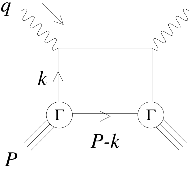
Figure 1:

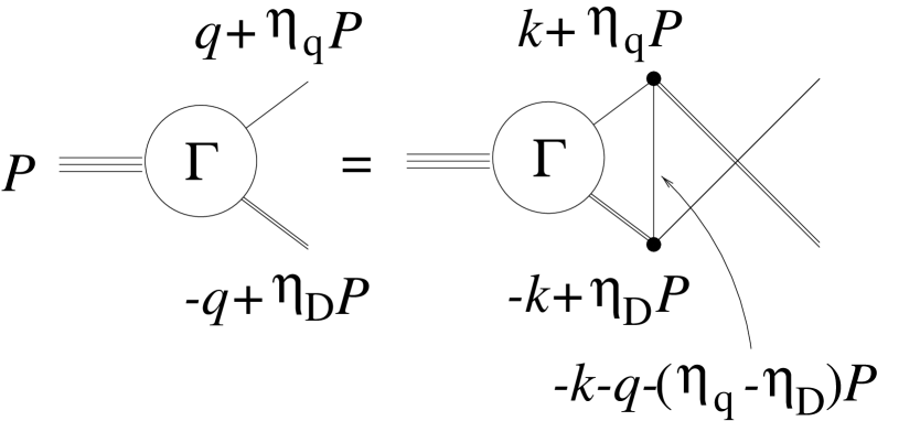
Figure 2:

Figure 3:

Figure 4:

Figure 5:

Figure 6:

Figure 7:

References

- [1] R.L. Jaffe, Phys. Rev. D11, 1953 (1975).
- [2] A.W. Schreiber, A.W. Thomas and J.T. Londergan, Phys. Lett. B237, 120 (1989); Phys. Rev. D42, 2226 (1990); A.I. Signal and A.W. Thomas, Phys. Rev. D40, 2832 (1989).
- [3] H. Meyer and P.J. Mulders, Nucl. Phys. A528, 589 (1991).
- [4] W. Melnitchouk, A.W. Schreiber and A.W. Thomas, Phys. Rev. D49, 1183 (1994), Phys. Lett. B335, 11 (1994).
- [5] W. Melnitchouk, G. Piller and A.W. Thomas, Phys. Lett. B346, 165 (1995).
- [6] A. Buck, R. Alkofer and H. Reinhardt, Phys. Lett. B286, 29 (1992).
- [7] S. Huang and J. Tjon, Phys. Rev. C49, 1702 (1994).
- [8] H. Asami, N. Ishii, W. Bentz and K. Yazaki, Phys. Rev. C51, 3388 (1995).
- [9] A.R. Edmonds, Angular momentum in quantum mechanics, (Princeton Univ. Press, 1957).
- [10] A. Erdelyi, et. al., Higher Transcendental Functions (McGraw-Hill Book Company Inc., New York, 1953).
- [11] K. Rothe, Phys. Rev. 170, 1548 (1968).
- [12] K. Ladanyi, Nucl. Phys. B57, 221 (1973).
- [13] N. Nakanishi, Suppl. Prog. Theor. Phys. 43, 1 (1969).
- [14] E. zur Linden and H. Mitter, Nuovo Cim. 61B, 389 (1969).
- [15] P. Jain and H.J. Munczek, Phys. Rev. D48, 5403 (1993).
- [16] M.L. Goldberger and K.M. Watson, Collision Theory (Wiley, New York, 1964).
- [17] G. Domokos, Phys. Rev. 159, 1387 (1967).
- [18] M.L. Goldberger, D.E. Soper and A.H. Guth, Phys. Rev. D14, 1117 (1976).
- [19] M.L. Goldberger, D.E. Soper and A.H. Guth, Phys. Rev. D14, 2633 (1976).
- [20] K. Kusaka and A. G. Williams, Phys. Rev. D51, 7026 (1995).