Electric-Magnetic Duality and the Heavy Quark Potential

Abstract

We use the assumption of electric-magnetic duality to express the heavy quark potential in QCD in terms of a Wilson Loop $W_{\mbox{\scriptsize eff}}(\Gamma)$ determined by the dynamics of a dual theory which is weakly coupled at long distances. The classical approximation gives the leading contribution to $W_{\mbox{\scriptsize eff}}(\Gamma)$ and yields a velocity dependent heavy quark potential which for large $R$ becomes linear in $R$, and which for small $R$ approaches lowest order perturbative QCD. The corresponding long distance interaction between color magnetic monopoles is governed by a Yukawa potential. As a consequence the magnetic interaction between the color magnetic moments of the quarks is exponentially damped. The semi-classical corrections to $W_{\mbox{\scriptsize eff}}(\Gamma)$ due to fluctuations of the classical flux tube should lead to an effective string theory free from the conformal anomaly.

1 Introduction

In this talk we will describe how to calculate the Wilson loop $W(\Gamma)$ determining the spin dependent, velocity dependent heavy quark potential $V_{q\bar{q}}$ using the assumption of electric-magnetic duality; namely, that the long distance physics of Yang Mills theory depending upon strongly coupled gauge potentials $A_{\mu}$ is the same as the long distance physics of a dual theory describing the interactions of weakly coupled dual potentials $C_{\mu}$ and monopole fields $B_{i}$. To calculate $V_{q\bar{q}}$ at long distances we replace $W(\Gamma)$ by $W_{\mbox{\scriptsize eff}}(\Gamma)$ a functional integral over the variables of the dual theory [1]. Because the long distance fluctuations of the dual variables are small we can use a semi-classical expansion to evaluate $W_{\mbox{\scriptsize eff}}$. The classical approximation gives the dual superconductor picture of confinement [2] and the semi-classical corrections lead to an effective string theory [3]. We first review electric-magnetic duality in electrodynamics.

2 Electric-Magnetic Duality in Electrodynamics

Consider a pair of particles with charges $e(-e)$ moving along trajectories $\vec{z}_{1}(t)(\vec{z}_{2}(t))$ in a relativistic medium having dielectric constant $\epsilon$. The trajectories $\vec{z}_{1}(t)(\vec{z}_{2}(t))$ define world lines $\Gamma_{1}(\Gamma_{2})$ running from $t_{i}$ to $t_{f}(t_{f}$ to $t_{i})$. The world lines $\Gamma_{1}(\Gamma_{2})$, along with two straight lines at fixed time connecting $\vec{y}_{1}$ to $\vec{y}_{2}$ and $\vec{x}_{1}$ to $\vec{x}_{2}$, then make up a closed contour $\Gamma$ (See Fig.1). The current density $j^{\mu}(x)$ then has the form

$$j^{\mu}(x)=e\oint_{\Gamma}dz^{\mu}\delta(x-z).$$ (1)

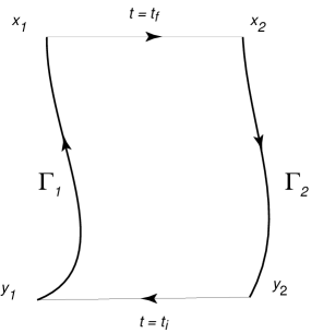
Figure 1: The loop $\Gamma$.

In the usual $A_{\mu}$ (electric) description this system is described by a Lagrangian

$${\cal L}_{A}(j)=-{\epsilon\over 4}(\partial_{\alpha}A_{\beta}-\partial_{\beta}A_{\alpha})^{2}-j^{\alpha}A_{\alpha}.$$ (2)

Then

$$\int dx{\cal L}_{A}(j)=-\int dx{\epsilon(\partial_{\mu}A_{\nu}-\partial_{\nu}A_{\mu})^{2}\over 4}-e\oint_{\Gamma}dz^{\mu}A_{\mu}(z).$$ (3)

The functional integral defining $W(\Gamma)$ in electrodynamics is

$$W(\Gamma)={\int{\cal D}A_{\mu}e^{i\int dx[{\cal L}_{A}(j)+{\cal L}_{GF}]}\over\int{\cal D}A_{\mu}e^{i\int dx[{\cal L}_{A}(j=0)+{\cal L}_{GF}]}},$$ (4)

where ${\cal L}_{GF}$ is a gauge fixing term.

The spin independent electron positron potential $V_{e^{+}e^{-}}(\vec{R},{\dot{\vec{z}}}_{1},{\dot{\vec{z}}}_{2})$ is obtained from the expansion of $i$ log $W(\Gamma)$ to second order in the velocities ${\dot{\vec{z}}}_{1}$ and ${\dot{\vec{z}}}_{2}$ by the equation:

$$i\log W(\Gamma)=\int_{t_{i}}^{t_{f}}dtV_{e^{+}e^{-}}(\vec{R},{\dot{\vec{z}}}_{1},{\dot{\vec{z}}}_{2})\,,$$ (5)

where $\vec{R}=\vec{z}_{1}(t)-\vec{z}_{2}(t)$. To higher order in the velocities, $i$ log $W(\Gamma)$ cannot be written in the above form and the concept of a potential is not defined because of the occurence of radiation. Eq.(5) does not include contributions of closed loops of electron positron pairs to $V_{e^{+}e^{-}}$.

The integral (4) is gaussian and has the value

$$W(\Gamma)=e^{-{ie^{2}\over 2}\int_{\Gamma}dx^{\mu}\int_{\Gamma}dx^{\prime\nu}{D_{\mu\nu}(x-x^{\prime})\over\epsilon}},$$ (6)

where $D_{\mu\nu}$ is the free photon propagator. Letting $\epsilon=1$ and expanding $i\log W(\Gamma)$ to second order in the velocities gives: [4]

$$V_{e^{+}e^{-}}=-{e^{2}\over 4\pi R}+{1\over 2}{e^{2}\over 4\pi R}\left[{\dot{\vec{z}}}_{1}\cdot{\dot{\vec{z}}}_{2}+{({\dot{\vec{z}}}_{1}\cdot\vec{R})({\dot{\vec{z}}}_{2}\cdot\vec{R})\over R^{2}}\right]\equiv V_{D}.$$ (7)

Furthermore the spin dependent electron positron potential $V_{e^{+}e^{-}}^{\mbox{\scriptsize spin}}$ is determined by the expectation value $\langle\langle F_{\mu\nu}\rangle\rangle_{Maxwell}$ of the electromagnetic field in the presence of the external current (1).

In the dual description first we write the inhomogeneous Maxwell equations in the form:

$$-\partial^{\beta}{\epsilon_{\alpha\beta\sigma\lambda}G^{\sigma\lambda}\over 2}=j_{\alpha},$$ (8)

where $G_{\mu\nu}$ is the dual field tensor composed of the electric displacement vector $\vec{D}$ and the magnetic field vector $\vec{H}$:

$$G_{0k}\equiv H_{k},\qquad G_{\ell m}\equiv\epsilon_{\ell mn}D^{n}.$$ (9)

Next attach a line $L$ of polarization charge between the electron positron pair. As the charges move the line $L$ sweeps out a surface $y^{\alpha}\left(\sigma,\tau\right)$ bounded by $\Gamma$ (the Dirac sheet) and generates the Dirac polarization tensor $G_{\mu\nu}^{S}\left(x\right)$: [5]

$$G_{\mu\nu}^{S}(x)=-e\epsilon_{\mu\nu\alpha\beta}\int d\sigma\int d\tau{\partial y^{\alpha}\over\partial\sigma}{\partial y^{\beta}\over\partial\tau}\delta(x-y(\sigma,\tau)).$$ (10)

The current density (1) can then be written in the form: [5]

$$-\partial^{\beta}{\epsilon_{\alpha\beta\sigma\lambda}G^{S\sigma\lambda}(x)\over 2}=j_{\alpha}(x),$$ (11)

and the solution of the inhomogeneous Maxwell equations (8) is

$$G_{\mu\nu}=\partial_{\mu}C_{\nu}-\partial_{\nu}C_{\mu}+G_{\mu\nu}^{S},$$ (12)

which defines the magnetic variables (the dual potentials $C_{\mu}$).

The homogeneous Maxwell equations for $\vec{E}$ and $\vec{B}$, written in the form

$$\partial^{\alpha}(\mu G_{\alpha\beta})=0,$$ (13)

where $\mu={1\over\epsilon}$ is the magnetic susceptibility, become dynamical equations for the dual potentials, and can be obtained by varying $C_{\mu}$ in the Lagrangian

$${\cal L}_{C}(G_{\mu\nu}^{S})=-{1\over 4}\mu G_{\mu\nu}G^{\mu\nu}\,,$$ (14)

where $G_{\mu\nu}$ is given by (12). This Lagrangian provides the dual (magnetic) description of the Maxwell theory (2). In the dual description the Wilson loop $W(\Gamma)$ is given by

$$W(\Gamma)={\int{\cal D}C_{\mu}e^{i\int dx[{\cal L}_{C}(G_{\mu\nu}^{S})+{\cal L}_{GF}]}\over\int{\cal D}C_{\mu}e^{i\int dx[{\cal L}_{C}(G_{\mu\nu}^{S}=0)+{\cal L}_{GF}]}}.$$ (15)

The functional integral (15) is also Gaussian and has the value (6) with $1\over\epsilon$ replaced by $\mu$. We then have two equivalent descriptions at all distances of the electromagnetic interaction of two charged particles.

Note from (2) and (14) that the equations

$$\epsilon={1\over g_{el}^{2}},\hskip 18.06749pt\mu={1\over g_{mag}^{2}}$$ (16)

define electric and magnetic coupling constants. If the wave number dependent dielectric constant $\epsilon\rightarrow 0$ at long distances, then $g_{el}\rightarrow\infty$ and the Maxwell potentials $A_{\mu}$ are strongly coupled. By contrast, $g_{mag}\rightarrow 0$, and the dual potentials are weakly coupled at large distances.

3 The Heavy Quark Potential in QCD

The heavy quark potential $V_{q\bar{q}}$ is determined by the Wilson loop $W(\Gamma)$ of Yang Mills theory:

$$W(\Gamma)={\int{\cal D}Ae^{iS_{YM}(A)}trP\exp(-ie\oint_{\Gamma}dx^{\mu}A_{\mu}(x))\over\int{\cal D}Ae^{iS_{YM}(A)}}.$$ (17)

(See Fig.1) As usual $A_{\mu}(x)={1\over 2}\lambda_{a}A_{\mu}^{a}(x)$, $tr$ means the trace over color indices, $P$ prescribes the ordering of the color matrices according to the direction fixed on the loop and $S_{YM}(A)$ is the Yang–Mills action including a gauge fixing term. We have denoted the Yang–Mills coupling constant by e, i.e.,

$$\alpha_{s}={e^{2}\over 4\pi}.$$ (18)

The spin independent part $V(\vec{R},{\dot{\vec{z}}}_{1},{\dot{\vec{z}}}_{2})$ of $V_{q\bar{q}}$ is obtained from (17) by the QCD analogue of (5):

$$i\log W(\Gamma)=\int_{t_{i}}^{t_{f}}dtV(\vec{R},{\dot{\vec{z}}}_{1},{\dot{\vec{z}}}_{2}).$$ (19)

The spin dependent heavy quark potential $V^{\mbox{\scriptsize spin}}$ is a sum of terms depending upon quark spin matrices, masses, and momenta: [1]

$$V^{\mbox{\scriptsize spin}}=V_{LS}^{MAG}+V_{Thomas}+V_{Darwin}+V_{SS},$$ (20)

where the notation indicates the physical significance of the individual terms (MAG denotes magnetic). Each term in (20) can be obtained from a corresponding term in $V_{e^{+}e^{-}}^{\mbox{\scriptsize spin}}$ by making the replacement

$$\langle\langle F_{\mu\nu}\left(z_{1}\right)\rangle\rangle_{Maxwell}\longrightarrow\langle\langle F_{\mu\nu}\left(z_{1}\right)\rangle\rangle_{YM},$$ (21)

where

$$\langle\langle F_{\mu\nu}\left(z_{1}\right)\rangle\rangle_{YM}\equiv{\int{\cal D}Ae^{iS_{YM}(A)}trP\exp[-ie\oint_{\Gamma}dx^{\mu}A_{\mu}(x)]F_{\mu\nu}\left(z_{1}\right)\over\int{\cal D}Ae^{iS_{YM}(A)}trP\exp[-ie\oint_{\Gamma}dx^{\mu}A_{\mu}(x)]},$$ (22)

and

$$F_{\mu\nu}=\partial_{\mu}A_{\nu}-\partial_{\nu}A_{\mu}-ie[A_{\mu},A_{\nu}],$$ (23)

i.e. $\langle\!\langle F_{\mu\nu}(x)\rangle\!\rangle_{YM}$ is the expectation value of the Yang–Mills field tensor in the presence of a quark and anti–quark moving along classical trajectories $\vec{z}_{1}(t)$ and $\vec{z}_{2}(t)$ respectively.

The calculation of the heavy quark potential is then reduced to the evaluation of functional integrals of Yang Mills theory. Because of the strong coupling at long distances all field configurations can give important contributions to (17) and (22) for large loops $\Gamma$ and there is no simple description in terms of Yang Mills potentials.

4 The Dual Description of Long Distance Yang-Mills Theory

The dual theory described here is a concrete realization of the Mandelstam ’t Hooft [2] dual superconductor picture of confinement. A dual Meissner effect prevents the electric color flux from spreading out as the distance $R$ between the quark anti-quark pair increases. As a result a linear potential develops which confines the quarks in hadrons. Such a dual picture is suggested by the solution of a truncated set of Dyson equations of Yang Mills theory [6] which gives an effective dielectric constant $\epsilon(q)\rightarrow q^{2}/M^{2}$ as $q^{2}\rightarrow 0$ ($M$ is an undetermined mass scale). As a consequence $\mu={1\over\epsilon}\rightarrow{M^{2}\over q^{2}}$ as $q^{2}\rightarrow 0$ so that the dual gluon becomes massive as is characteristic of dual superconductivity. However, such a truncation cannot be justified in the strongly coupled domain and duality in Yang Mills theory remains an hypothesis.

On the other hand, there has been a recent revival of interest in electric-magnetic duality due to the work of Seiberg and Witten [7] on supersymmetric $N=2$ Yang Mills theory and Seiberg [8] on $N=1$ supersymmetric QCD. The long distance physics of these models, which are asymptotically free, is described by weakly coupled dual gauge theories. These examples of non-Abelian gauge theories for which duality can can be inferred provide new motivation for the duality hypothesis for Yang Mills theory.

The dual theory is described by an effective Lagrangian density ${\cal L}_{\mbox{\scriptsize eff}}$ in which the fundamental variables are an octet of dual potentials ${\bf C_{\mu}}$ coupled minimally to three octets of scalar Higgs fields ${\bf B}_{i}$ carrying magnetic color charge [1, 9]. (The gauge coupling constant of the dual theory $g={2\pi\over e}$). The Higgs potential has a minimum at non-zero values ${\bf B}_{0i}$ which have the color structure

$${\bf B}_{01}=B_{0}\lambda_{7},\quad{\bf B}_{02}=B_{0}(-\lambda_{5}),\quad{\bf B}_{03}=B_{0}\lambda_{2}.$$ (24)

The three matrices $\lambda_{7},-\lambda_{5}$ and $\lambda_{2}$ transform as a $j=1$ irreducible representation of an $SU(2)$ subgroup of $SU(3)$ and as there is no $SU(3)$ transformation which leaves all three ${\bf B}_{0i}$ invariant the dual $SU(3)$ gauge symmetry is completely broken and the eight Goldstone bosons become the longitudinal components of the now massive $\bf{C}_{\mu}$.

The basic manifestation of the dual superconducting properties of ${\cal L}_{\mbox{\scriptsize eff}}$ is that it generates classical equations of motion having solutions [10] carrying a unit of $Z_{3}$ flux confined in a narrow tube along the $z$ axis (corresponding to having quark sources at $z=\pm\infty$). (These solutions are dual to Abrikosov-Nielsen-Olesen magnetic vortex solutions [11] in a superconductor). Before writing ${\cal L}_{\mbox{\scriptsize eff}}$ we briefly describe these classical solutions. The monopole fields ${\bf B}_{i}$ have the form : [1]

$${\bf B}_{1} = B_{1}(x)\lambda_{7}+\bar{B}_{1}(x)(-\lambda_{6})\,,$$

$${\bf B}_{2} = B_{2}(x)(-\lambda_{5})+\bar{B}_{2}(x)\lambda_{4}\,,$$ (25)

$${\bf B}_{3} = B_{3}(x)\lambda_{2}+\bar{B}_{3}(x)(-\lambda_{1})\,.$$

We denote

$$\phi_{i}(x)=B_{i}(x)-i\bar{B}_{i}(x)\,,$$ (26)

and look for solutions where the dual potential is proportional to the hypercharge matrix $Y={\lambda_{8}\over\sqrt{3}}$,

$${\bf C}_{\mu}=C_{\mu}Y,$$ (27)

and where

$$\phi_{1}(x)=\phi_{2}(x)\equiv\phi(x),\hskip 18.06749pt\phi_{3}(x)=B_{3}(x).$$ (28)

At large distances from the center of the flux tube in cylindrical coordinates $\rho,\theta,z$ the boundary conditions are:

$$\vec{C}\rightarrow-{\hat{e}_{\theta}\over g\rho},\quad~{}\phi\rightarrow B_{0}e^{i\theta},\quad B_{3}\rightarrow B_{0},~{}\quad\mbox{as}\ ~{}\rho\rightarrow\infty.$$ (29)

The non-vanishing of $B_{0}$ produces a color monopole current confining the electric color flux. The line integral of the dual potential around a large loop surrounding the $z$ axis measures this flux, and the boundary condition (29) for $\vec{\bf C}$ gives

$$e^{-ig\oint_{loop}\vec{\bf C}\cdot d\vec{\ell}}=e^{2\pi iY}=e^{2\pi\left({i\over 3}\right)},$$ (30)

which manifests the unit of $Z_{3}$ flux in the tube. The energy per unit length in this flux tube gives the string tension $\sigma$: [10]

$$\sigma\sim 24B_{0}^{2}.$$ (31)

The field $\phi(\vec{x})$ vanishes at the center of the flux tube. By contrast $B_{3}(\vec{x})$ does not couple to quarks and remains close to its vacuum value for all $\vec{x}$. For simplicity in the rest of this talk we set $B_{3}(x)=B_{0}$, in which case ${\cal L}_{\mbox{\scriptsize eff}}$ reduces to the Abelian Higgs model.

To couple ${\bf C}_{\mu}$ to a $q\bar{q}$ pair separated by a finite distance we represent quark sources by a Dirac string tensor ${\bf G}_{\mu\nu}^{S}$. We choose the dual potential to have the same color structure (27) as the flux tube solution. Then ${\bf G}_{\mu\nu}^{S}$ must also be proportional to the hypercharge matrix,

$${\bf G}_{\mu\nu}^{S}=YG_{\mu\nu}^{S},$$ (32)

where $G_{\mu\nu}^{S}$ is given by (10), so that one unit of $Z_{3}$ flux flows along the Dirac string connecting the quark and anti-quark. With the ansaetze (32) and (25)- (28) along with the simplification $B_{3}(x)=B_{0}$ , the Lagrangian density ${\cal L}_{\mbox{\scriptsize eff}}\left(G_{\mu\nu}^{S}\right)$ coupling dual potentials to classical quark sources moving along trajectories $\vec{z}_{1}(t)$ and $\vec{z}_{2}(t)$ assumes the form:

$${\cal L}_{\mbox{\scriptsize eff}}(G_{\mu\nu}^{S})=-{4\over 3}{\left(G_{\mu\nu}G^{\mu\nu}\right)\over 4}+{8|(\partial_{\mu}-igC_{\mu})\phi|^{2}\over 2}-{100\over 3}\lambda\left(|\phi|^{2}-B_{0}^{2}\right)^{2},$$ (33)

where

$$G_{\mu\nu}=\partial_{\mu}C_{\nu}-\partial_{\nu}C_{\mu}+G_{\mu\nu}^{S}\,,$$ (34)

and

$$g={2\pi\over e}.$$ (35)

The first term in ${\cal L}_{\mbox{\scriptsize eff}}$ is the coupling of dual potentials to quarks, the second is the coupling of the dual potentials to monopole fields $\phi$, while the third term is the quartic self coupling of the monopole fields. The numerical factors in (33) arise from inserting the color structures (25)- (28) in the original non-Abelian form of ${\cal L}_{\mbox{\scriptsize eff}}$. By a suitable redefinition of $\phi$ and $\lambda$ the last two terms can be written in the standard form of the Abelian Higgs model, while the color factor $4\over 3$ in the first term is a consequence of (27) and (32), which combined with the boundary condition (29) provides the unit of $Z_{3}$ flux.

We find from (33) the following values of the dual gluon mass $M$ and the monopole mass $M_{\phi}$ :

$$M^{2}=6g^{2}B_{0}^{2}\hskip 10.84006pt,\hskip 18.06749ptM_{\phi}^{2}={100\lambda\over 3}B_{0}^{2}.$$ (36)

The quantity $g^{2}/\lambda$ plays the role of a Landau-Ginzburg parameter. Its value can be estimated by relating the difference between the energy density at a large distance from the flux tube and the energy density at its center to the gluon condensate.[10] This procedure gives $g^{2}/\lambda\simeq 5$. There remain two free parameters in ${\cal L}_{\mbox{\scriptsize eff}}$, which we take to be $\alpha_{s}={e^{2}\over 4\pi}={\pi\over g^{2}}$ and the string tension $\sigma$.

We denote by $W_{\mbox{\scriptsize eff}}(\Gamma)$ the Wilson loop of the dual theory, i.e.,

$$W_{\mbox{\scriptsize eff}}(\Gamma)={\int{\cal D}C_{\mu}{\cal D}\phi e^{i\int dx[{\cal L}_{\mbox{\scriptsize eff}}(G_{\mu\nu}^{S})+{\cal L}_{GF}]}\over\int{\cal D}C_{\mu}{\cal D}\phi e^{i\int dx[{\cal L}_{\mbox{\scriptsize eff}}(G_{\mu\nu}^{S}=0)+{\cal L}_{GF}]}}.$$ (37)

The functional integral $W_{\mbox{\scriptsize eff}}(\Gamma)$ determines in the effective dual theory the same physical quantity as $W(\Gamma)$ in Yang-Mills theory, namely the action for a quark anti-quark pair moving along classical trajectories. The coupling of dual potentials to Dirac strings in ${\cal L}_{\mbox{\scriptsize eff}}\left(G_{\mu\nu}^{S}\right)$ plays the role in eq.(37) for $W_{\mbox{\scriptsize eff}}(\Gamma)$ of the Wilson loop $Pe^{-ie\oint_{\Gamma}dx^{\mu}A_{\mu}(x)}$ in eq.(17) for $W(\Gamma)$.

The assumption that the dual theory describes the long distance $q\bar{q}$ interaction in Yang-Mills theory then takes the form:

$$W(\Gamma)=W_{\mbox{\scriptsize eff}}(\Gamma),~{}{\rm for~{}large~{}loops~{}\Gamma}.$$ (38)

Large loops mean that the size $R$ of the loop is large compared to the inverse of $M$ and $M_{\phi}$. Since the dual theory is weakly coupled at large distances we can evaluate $W_{\mbox{\scriptsize eff}}(\Gamma)$ via a semi-classical expansion to which the classical configuration of dual potentials and monopoles gives the leading contribution. Furthermore using (38), we can relate the expectation value (22) of the Yang Mills Field tensor at the position of a quark to the corresponding expectation value of the dual field tensor in the effective theory: [1]

$$\langle\langle F_{\mu\nu}(z_{1})\rangle\rangle_{YM}={4\over 3}\langle\langle\hat{G}_{\mu\nu}(z_{1})\rangle\rangle_{\mbox{\scriptsize eff}},$$ (39)

where

$$\hat{G}_{\mu\nu}(x)\equiv{1\over 2}\epsilon_{\mu\nu\lambda\sigma}G^{\lambda\sigma}(x),$$ (40)

and

$$\langle\!\langle G^{\mu\nu}(z_{1})\rangle\!\rangle_{\mbox{\scriptsize eff}}\equiv{\int{\cal D}C_{\mu}{\cal D}\phi e^{i\int dx({\cal L}_{\mbox{\scriptsize eff}}(G_{\mu\nu}^{S})+{\cal L}_{GF})}G^{\mu\nu}(z_{1})\over\int{\cal D}C_{\mu}{\cal D}\phi e^{i\int dx({\cal L}_{\mbox{\scriptsize eff}}(G_{\mu\nu}^{S})+{\cal L}_{GF})}}.$$ (41)

To obtain the spin independent heavy quark potential $V({\vec{R}},{\dot{\vec{z}}}_{1},{\dot{\vec{z}}}_{2})$ in the dual theory we replace $W(\Gamma)$ by $W_{\mbox{\scriptsize eff}}(\Gamma)$ in eq.(19). This expresses the spin independent heavy quark potential in terms of the zero order and quadratic terms in the expansion of $i\log W_{\mbox{\scriptsize eff}}(\Gamma)$ for small velocities ${\dot{\vec{z}}}_{1}$ and ${\dot{\vec{z}}}_{2}$. The corresponding spin dependent potential in the dual theory is obtained by making the replacement

$$\langle\langle F_{\mu\nu}(z_{1})\rangle\rangle_{YM}\longrightarrow\hskip 10.84006pt{4\over 3}\langle\langle\hat{G}_{\mu\nu}(z_{1})\rangle\rangle_{\mbox{\scriptsize eff}},$$ (42)

in the expressions in eq.(20) for $V^{\mbox{\scriptsize spin}}$.

5 The Classical Approximation to the Dual Theory

In the classical approximation all quantities are replaced by their classical values

$$\langle\langle G_{\mu\nu}(x)\rangle\rangle_{\mbox{\scriptsize eff}}=G_{\mu\nu}(x),\hskip 18.06749pti\log W_{\mbox{\scriptsize eff}}=-\int dx{\cal L}_{\mbox{\scriptsize eff}}(G_{\mu\nu}^{S}),$$ (43)

where $G_{\mu\nu}$ and ${\cal L}_{\mbox{\scriptsize eff}}\left(G_{\mu\nu}^{S}\right)$ are evaluated at the solution of the classical equations of motion:

$$\partial^{\alpha}\left(\partial_{\alpha}C_{\beta}-\partial_{\beta}C_{\alpha}\right)=-\partial^{\alpha}G_{\alpha\beta}^{S}+j_{\beta}^{MON},$$ (44)

$$\left(\partial_{\mu}-igC_{\mu}\right)^{2}\phi=-{200\lambda\over 3}\phi\left(|\phi|^{2}-B_{0}^{2}\right),$$ (45)

where the monopole current $j_{\mu}^{MON}$ is

$$j_{\mu}^{MON}=-3ig[\phi^{*}\left(\partial_{\mu}-igC_{\mu}\right)\phi-\phi\left(\partial_{\mu}+igC_{\mu}\right)\phi^{*}].$$ (46)

The boundary conditions on $\phi$ are:

$$\phi(x)\rightarrow 0,\quad\mbox{as}\ x\rightarrow y\left(\sigma,\tau\right);\qquad\phi(x)\rightarrow B_{0}\,,\quad\mbox{as}\ x\rightarrow\infty.$$ (47)

The vanishing of $\phi(x)$ on the Dirac sheet $y^{\mu}(\sigma,\tau)$ produces a flux tube with energy concentrated in the neighborhood of the string connecting the quark anti-quark pair. Using the minimum energy solution corresponding to a straight line string , we evaluate $i\log W_{\mbox{\scriptsize eff}}$ to second order in the velocities ${\dot{\vec{z}}}_{1},$ and ${\dot{\vec{z}}}_{2}$ and obtain the spin independent heavy quark potential.

At large separations $V(\vec{R},{\dot{\vec{z}}}_{1},{\dot{\vec{z}}}_{2})$ is linear in $R$ since the monopole current screens the color field of the quarks so that a color electric Abrikosov-Nielsen-Olesen vortex forms between the moving $q\bar{q}$ pair. For the case of circular motion, $({\dot{\vec{z}}}_{i}\cdot\vec{R}=0$, ${\dot{\vec{z}}}_{2}=-{\dot{\vec{z}}}_{1})$, we find:

$$V\rightarrow\sigma R\left[1-A{(\dot{\vec{z}_{1}}\times\vec{R})^{2}\over R^{2}}\right]\,,\quad\mbox{as}\ R\rightarrow\infty\,,$$ (48)

where

$$A\simeq.21\sigma.$$ (49)

The constant $A$ determines the long distance moment of inertia $I(R)$ of the rotating flux tube:

$$\lim_{R\rightarrow\infty}I(R)={1\over 2}(AR)R^{2}.$$ (50)

At small separations the color field generated by the quarks expels the monopole condensate from the region between them and as $R\rightarrow 0$, $V$ approaches the one gluon exchange result, ${4\over 3}V_{D}$. See eq.(7).

As the simplest application of this potential, we add relativistic kinetic energy terms to obtain a classical Lagrangian, and calculate classically the energy and angular momentum of $q\bar{q}$ circular orbits, which are those which have the largest angular momentum $J$ for a given energy. We find [12] a Regge trajectory $J$ as a function of $E^{2}$ which for large $E^{2}$ becomes linear with slope $\alpha^{\prime}=J/E^{2}=1/8\sigma\left(1-A/\sigma\right)$. Then (49) gives $\alpha^{\prime}\approx 1/6.3\sigma$, which is close to the string model relation $\alpha^{\prime}={1\over 2\pi\sigma}$. This comparison shows how at the classical level a string model emerges when the velocity dependence of the $q\bar{q}$ potential is included.

To calculate the spin dependent heavy quark potential we use (42) and (43) to evaluate $V^{\mbox{\scriptsize spin}}$ (20) in the classical approximation to the dual theory. The resulting expressions are given in reference 1. Here we discuss only the result for the spin-spin interaction $V_{SS}^{\mbox{\scriptsize spin}}$ between the color magnetic moments of the quark anti-quark pair. This magnetic dipole interaction is determined by the gradient of the Greens function $G\left(\vec{x},\vec{x}^{\prime}\right)$ describing the interaction of monopoles:

$$V_{SS}^{\mbox{\scriptsize spin}}={4\over 3}{e^{2}\over m_{1}m_{2}}\Bigg{\{}(\vec{S}_{1}\cdot\vec{S}_{2})\delta(\vec{z}_{1}-\vec{z}_{2})-{(\vec{S}_{1}\cdot\vec{\nabla})(\vec{S}_{2}\cdot\vec{\nabla}^{\prime})}G(\vec{x},\vec{x}^{\prime})\Bigg{|}_{\vec{x}=\vec{z}_{1},\vec{x}^{\prime}=\vec{z}_{2}}\Bigg{\}}.$$ (51)

$G$ satisfies the following equation obtained from eq.(44) for $C^{0}$ :

$$[-\bigtriangledown^{2}+6g^{2}\phi^{2}(\vec{x})]G\left(\vec{x},\vec{x}^{\prime}\right)=\delta\left(\vec{x}-\vec{x}^{\prime}\right)\,,$$ (52)

where $\phi(\vec{x})$ is the static monopole field. ($\phi(x)$ is real so that the monopole charge density $j^{0}(x)=6g^{2}\phi^{2}(x)C^{0}$.) Since $\phi(\vec{x})$ approaches its vacuum value $B_{0}$ as $\vec{x}\rightarrow\infty$, $G$ vanishes exponentially at large distances:

$$G(\vec{x},\vec{x}^{\prime})\mathrel{\mathop{\longrightarrow}_{\vec{x}\to\infty}}{e^{-M|\vec{x}-\vec{x}^{\prime}|}\over 4\pi|\vec{x}-\vec{x}^{\prime}|}\,.$$ (53)

See eq.(36).

The dual Higgs mechanism then produces the long distance Yukawa potential (53) between monopoles along with the linear potential (48) between quarks. The resulting suppression of the color magnetic interaction between quarks is an unambiguous prediction of electric-magnetic duality.

6 Fluctuations of the Flux Tube and Effective String Theory

To evaluate the contributions to $W_{\mbox{\scriptsize eff}}$ arising from fluctuations of the shape and length of the flux tube we must integrate over field configurations generated by all strings connecting the $q\bar{q}$ pair. This amounts to doing a functional integral over all polarization tensors $G_{\mu\nu}^{S}(x)$. Similar integrals have recently been carried out by Akhmedov et al. [3] in the case $\lambda\rightarrow\infty$. By changing from field variables to string variables ,the functional integral over $G_{\mu\nu}^{S}(x)$ is replaced by a functional integral over corresponding world sheets $y^{\mu}\left(\sigma,\tau\right)$, multipled by an appropriate Jacobian and there results [3] an effective string theory free from the conformal anomaly [13] Such techniques if extended to finite $\lambda$ could be applied to $W_{\mbox{\scriptsize eff}}$ to obtain a corresponding effective string theory . The leading long distance contribution to the static potential due to fluctuations of the string which is independent of the details of the string theory would then have the universal value $-{\pi\over 12R}$. [14]

7 Conclusion

We have obtained an expression for the heavy quark potential $V_{q\bar{q}}$ in terms of an effective Wilson loop $W_{\mbox{\scriptsize eff}}(\Gamma)$ determined by the dynamics of a dual theory which is weakly coupled at long distances. The classical approximation gives the leading long distance contribution to $W_{\mbox{\scriptsize eff}}(\Gamma)$ and yields a velocity dependent spin dependent heavy quark potential which for large $R$ becomes linear in $R$ and which for small $R$ approaches lowest order perturbative QCD. The dual theory cannot describe QCD at shorter distances, where radiative corrections giving rise to asymptotic freedom become important. At such distances the dual potentials are strongly coupled and the dual description is no longer appropriate.

As a final remark we note that the dual theory is an $SU(3)$ gauge theory, like the original Yang-Mills gauge theory. However, the coupling to quarks selected out only Abelian configurations of the dual potential. Therefore, our results for the $q\bar{q}$ interaction do not depend upon the details of the dual gauge group and should be regarded more as consequences of the general dual superconductor picture rather than of our particular realization of it.

8 Acknowledgments

I would like to thank N. Brambilla and G. M. Prosperi for the opportunity to attend this conference and for their important contributions to the work presented here.

9 References

References

• [1] M. Baker, J.S. Ball, N. Brambilla, G.M. Prosperi and F. Zachariasen, Phys. Rev. D 54, 2829 (1996).
• [2] S. Mandelstam, Phys. Rep. 23C, 145 (1976). G. โ€™t Hooft, in โ€œProc. Eur. Phys. Soc. 1975โ€ ed. by A. Zichichi (Ed. Comp. Bologna 1976) .
• [3] E.T. Akhmedov, M.N. Chernodub, M.I. Polikarpov and M. A. Zubkov, Phys. Rev. D 53, 2097 (1996).
• [4] G.G. Darwin, Phil. Mag. 39 , 537 (1920).
• [5] P.A.M. Dirac, Phys. Rev. 74 , 817 (1948).
• [6] S. Mandelstam, Phys. Rev. D 20, 3223 (1979); M. Baker, J.S. Ball and F. Zachariasen, Nucl. Phys. B 186, 531 (1981).
• [7] N. Seiberg and E. Witten, Nucl. Phys. B 426, 19 (1994); Nucl. Phys. B 431, 484 (1994).
• [8] N. Seiberg, Nucl. Phys. B 435, 129 (1995).
• [9] M. Baker, J.S. Ball and F. Zachariasen, Phys. Rev. D 51, 1968 (1995).
• [10] M. Baker, J.S. Ball and F. Zachariasen, Phys. Rev. D 41, 2612 (1990).
• [11] A.A. Abrikosov Sov. Phys. JETP 32, 1442 (1957); H.B. Nielsen and P. Olesen, Nucl. Phys. B 61, 45 (1973).
• [12] M. Baker in โ€œProceedings of the Workshop on Quantum Infrared Physicsโ€ Eds. H.M. Fried, B. Muller; World Scientific (1995), p.35.
• [13] A.M. Polyakov, Phys. Lett. B 103, 207 , 211 (1981).
• [14] M. Luscher, Nucl. Phys. B 180, 317 (1981).