Bologna preprint

DFUB-95-18

September 1995

GAUGE INVARIANCE ON BOUND STATE ENERGY LEVELS
Antonio Vairo

I.N.F.N. - Sez. di Bologna and Dip. di Fisica,
Università di Bologna, Via Irnerio 46, I-40126 Bologna, Italy

In this paper the problem of the gauge in a bound state calculation is discussed. In particular, in order to verify the gauge invariance in the energy levels expansion, some set of gauge invariant contributions are given.

1 Introduction

In this paper I review some basics concerning the gauge invariance on bound state  [1].

In the first section some simple examples about gauge invariance on mass-shell are given. In the second section there are some general considerations about gauge invariance in a off shell problem and up to order $\alpha^{4}$ the calculation of some contributions to the energy levels of positronium in Feynman gauge. The full cancellation of the spurious $\alpha^{3}\log\alpha$, $\alpha^{3}$ terms which arise typically in this gauge, is performed. The calculations are done in the Barbieri-Remiddi bound state formalism  [2],  [3]. $K_{c}$, $\psi_{c}$ are the Barbieri-Remiddi zeroth-order kernel and the corresponding wave function.

2 Gauge invariance on mass-shell.

It is generally easy to verify the gauge invariance in a scattering process. The incoming and outcoming particles are on mass-shell and the related wave functions are not $\alpha$-depending. This involves that each Feynman graph contributes to the scattering amplitude only at the order in the fine structure constant determined by his number of vertices. In the following I will verify the gauge invariance at the leading order in $\alpha$ in two very simply cases: the Compton and the $e^{+}~{}e^{-}$ scattering.

At the order $\alpha$ only the two graphs of Fig. 1 contribute to the Compton scattering amplitude.

b

Figure 1: Compton scattering at the tree level.

The contribution to the scattering amplitude coming from the graphs of Fig. 1 is:

$$A_{Com}(p_{1},k_{1};p_{2},k_{2}) = -(2\pi)^{4}\delta^{(4)}(p_{1}+k_{1}-p_{2}-k_{2})~{}\alpha$$

$$\cdot \Big{(}\bar{u}(p_{2}){\epsilon\kern-4.30554pt{/}}(k_{2})S_{F}(p_{1}+k_{1}){\epsilon\kern-4.30554pt{/}}(k_{1})u(p_{1})$$

$$+ ~{}\bar{u}(p_{2}){\epsilon\kern-4.30554pt{/}}(k_{1})S_{F}(p_{1}-k_{2}){\epsilon\kern-4.30554pt{/}}(k_{2})u(p_{1})\Big{)}~{},$$

where $k_{1}$, $p_{1}$ and $k_{2}$, $p_{2}$ are the incoming and outcoming momenta (on mass shell: $p_{j}^{2}=m^{2}$ for the electron momenta and $k_{j}^{2}=0$ for the photon momenta), $\epsilon^{\mu}$ is the photon polarization, $S_{F}$ the fermion free propagator:

$$S_{F}(p)={i\over{p\kern-4.30554pt{/}}-m+i\epsilon}~{},$$ (2.2)

and $u$, $\bar{u}$, $v$, $\bar{v}$ are the Dirac spinors ($({p\kern-4.30554pt{/}}-m)u(p)=0$, $({p\kern-4.30554pt{/}}+m)v(p)=0$).
The gauge variation (e.g. on the second external photon) of $A_{Com}$ i.e. $A_{Com}^{Gauge\#1}-A_{Com}^{Gauge\#2}$ is:

$$\delta A_{Com}(p_{1},k_{1};p_{2},k_{2}) = -(2\pi)^{4}\delta^{(4)}(p_{1}+k_{1}-p_{2}-k_{2})~{}\alpha$$

$$\cdot \bar{u}(p_{2})\Big{\{}{k\kern-5.16663pt{/}}_{2}S_{F}(p_{2}+k_{2}){\epsilon\kern-4.30554pt{/}}(k_{1})$$

$$+ {\epsilon\kern-4.30554pt{/}}(k_{1})S_{F}(p_{1}-k_{2}){k\kern-5.16663pt{/}}_{2}\Big{\}}u(p_{1})$$

$$= -(2\pi)^{4}\delta^{(4)}(p_{1}+k_{1}-p_{2}-k_{2})~{}\alpha$$

$$\cdot \bar{u}(p_{2})\Big{\{}\left(i-({p\kern-4.30554pt{/}}_{2}-m)S_{F}(p_{2}+k_{2})\right){\epsilon\kern-4.30554pt{/}}(k_{1})$$

$$+ {\epsilon\kern-4.30554pt{/}}(k_{1})\left(-i-S_{F}(p_{1}-k_{2})({p\kern-4.30554pt{/}}_{1}-m)\right)\Big{\}}u(p_{1})$$

$$= -(2\pi)^{4}\delta^{(4)}(p_{1}+k_{1}-p_{2}-k_{2})~{}\alpha$$

$$\cdot \bar{u}(p_{2})\Big{\{}i{\epsilon\kern-4.30554pt{/}}(k_{1})-i{\epsilon\kern-4.30554pt{/}}(k_{1})\Big{\}}u(p_{1})~{}=~{}0~{},$$

which verifies the gauge invariance.

The second example is the $e^{+}~{}e^{-}$ scattering amplitude. At the order $\alpha$ contributions to the scattering amplitude arise only from the graphs of Fig. 2.

b

Figure 2: $e^{+}~{}e^{-}$ scattering at the tree level.

The photon propagator $D_{\mu\nu}$ is gauge dependent; in Feynman and Coulomb gauge one can write it as:

$$D^{Fey}_{\mu\nu}(p) = -i{g_{\mu\nu}\over p^{2}+i\epsilon}~{};$$ (2.4)

$$D^{Cou}_{\mu\nu}(p) = -i{1\over p^{2}+i\epsilon}\left\{g_{\mu\nu}-{\eta\cdot p(p_{\mu}\eta_{\nu}+p_{\nu}\eta_{\mu})-p_{\mu}p_{\nu}\over{\vec{p}}^{~{}2}}\right\}$$ (2.5)

$$\eta^{\mu}=(1,\vec{0}~{})~{}.$$

The difference between the propagators in the above gauges can be expressed as:

$$D^{Cou}_{\mu\nu}(p)-D^{Fey}_{\mu\nu}(p) = b_{\mu}(p)p_{\nu}+b_{\nu}(p)p_{\mu}~{},$$

$$b_{\mu}(p) \equiv {i\over 2(p^{2}+i\epsilon)}{1\over\vec{p}^{~{}2}}(-p_{\mu}+2\delta_{0\mu}p_{0})~{}.$$ (2.6)

Not only the sum of the graphs in Fig. 2 is gauge invariant but each graph also. To verify the gauge invariance of the annihilation graph one needs only equation (2.6) and the Dirac equation for the spinors $u$ and $v$:

$$\delta A_{ann}(p_{1},k_{1};p_{2},k_{2}) = -(2\pi)^{4}\delta^{(4)}(p_{1}+k_{1}-p_{2}-k_{2})~{}\alpha$$

$$\cdot \bar{v}(k_{1})\gamma^{\mu}u(p_{1})\Big{\{}D^{Cou}_{\mu\nu}(p_{1}+k_{1})$$

$$- D^{Fey}_{\mu\nu}(p_{1}+k_{1})\Big{\}}\bar{u}(p_{2})\gamma^{\nu}v(k_{2})$$

$$= -(2\pi)^{4}\delta^{(4)}(p_{1}+k_{1}-p_{2}-k_{2})~{}\alpha$$

$$\cdot \bar{v}(k_{1})\gamma^{\mu}u(p_{1})\Big{\{}b_{\mu}(p_{1}+k_{1})~{}(p_{1\nu}+k_{1\nu})$$

$$+ b_{\nu}(p_{1}+k_{1})~{}(p_{1\mu}+k_{1\mu})\Big{\}}\bar{u}(p_{2})\gamma^{\nu}v(k_{2})$$

$$= -(2\pi)^{4}\delta^{(4)}(p_{1}+k_{1}-p_{2}-k_{2})~{}\alpha$$

$$\cdot \Big{(}\bar{v}(k_{1}){b\kern-4.30554pt{/}}(p_{1}+k_{1})~{}u(p_{1})\bar{u}(p_{2})({p\kern-4.30554pt{/}}_{2}+{k\kern-5.16663pt{/}}_{2})v(k_{2})$$

$$+ ~{}\bar{v}(k_{1})({p\kern-4.30554pt{/}}_{1}+{k\kern-5.16663pt{/}}_{1})u(p_{1})\bar{u}(p_{2}){b\kern-4.30554pt{/}}(p_{1}+k_{1})~{}v(k_{2})\Big{)}$$

$$= ~{}0~{}.$$

In the same way it is possible to prove the gauge invariance of the second graph of Fig. 2.

3 Gauge invariance on bound state.

The bound state wave function is $\alpha$-dependent. This is well-known for the Schrödinger-Coulomb wave function, but is also true for the Barbieri-Remiddi solution which reproduces it in the non relativistic limit. As a consequence of the non trivial $\alpha$-dependence each Feynman graph contributes to the energy levels perturbative expansion with a series in $\alpha$. Also the leading order of this series is not deductable in a trivial manner from a vertices counting. As a consequence in a relativistic bound state problem it is not possible to verify in a simply way, order by order in $\alpha$, the gauge invariance.

Although the difficulties to reconstruct sets of gauge invariant contributions, since some graphs give series which converge faster in $\alpha$ in a particular gauge than in an other, different gauges are used normally in the energy levels calculation. Typically binding photons (photons connecting fermion lines each other) are calculated in Coulomb gauge while annihilation and radiative ones in covariant gauge as the Feynman gauge. This not only in different graphs but also, where considered possible, in the same Feynman graph.

Such an approach is not free from ambiguities.

b

Figure 3: One-loop vertex corrections to the annihilation graph.

In Fig.3 there are drawn the vertex corrections at the one-photon annihilation graph. After regularization in order to obtain the UV-divergences cancellation it is necessary to consider together these three graphs, this means to use the same gauge for all the photons (see  [4]). If we use a covariant gauge for the radiative photons in the first two graphs the third one has to be also calculated in a covariant gauge. It follows that there are in any case some binding photons (as the no-annihilation photon of the third graph) which will be calculated in a covariant gauge.

In order to avoid these ambiguities and taking in account that the apparent simplicity of the Coulomb gauge seems to disappear in higher order calculations, a reference calculation of the energy levels has to be done in the Feynman gauge (or in an other covariant gauge). In the following I will show how the individuation of gauge invariant set of contributions can be helpful to cancel the low-order spurious terms arising in such an ab initio reference calculation.

The first contribution to the energy levels shift is coming from the one-photon exchange graph of Fig.4.

b

Figure 4: One-photon exchange graph.

On the positronium $1S$ state this graph contributes, in the Feynman gauge, as ($m=1$):

$$\langle\Gamma_{0}\rangle^{Fey}_{1S}=-{1\over 4}\alpha^{2}-{1\over 2\pi}\alpha^{3}\log\alpha+{1\over 4\pi}\alpha^{3}-{3\over 16}\alpha^{4}~{},$$ (3.1)

while in Coulomb gauge:

$$\langle\Gamma_{0}\rangle^{Cou}_{1S}=-{1\over 4}\alpha^{2}-{3\over 16}\alpha^{4}~{}.$$ (3.2)

As expected, and unlike the $e^{+}~{}e^{-}$ scattering, $\langle\Gamma_{0}\rangle$ is not gauge invariant: in Feynman gauge there are some contributions (the $\alpha^{3}\log\alpha$ and $\alpha^{3}$ terms) which are not in (3.2) and in the energy levels itself (it is well-known that the first correction to the Balmer’s levels is of order $\alpha^{4}$). To restore the gauge invariance there must exist some other contributions in the energy levels expansion which cancel in Feynman gauge these spurious terms. My principal purpose is from now to determine these other contributions. I preliminarily give the following general result.

If the zeroth-order kernel $K_{c}$ is local,

$$K_{c}({\vec{p}},{\vec{q}}~{})=K_{c}({\vec{p}}-{\vec{q}}~{})~{},$$ (3.3)

then:

$$\delta\langle\Gamma_{0}+2\sum_{n=1}^{\infty}I_{n}\rangle=0~{}.$$ (3.4)

In other words the sum of the contributions to the energy levels coming from $\Gamma_{0}$ and from the graphs of Fig.5 ($\times~{}2$) is gauge invariant.

b

Figure 5: $n$ kernel $K_{c}$ crossed by one photon.

In order to prove (3.4) first I give the gauge variation of $\langle I_{n}\rangle$:

$$\delta\langle I_{n}\rangle = \delta\langle K_{c}G_{0}I_{n}G_{0}K_{c}\rangle$$ (3.5)

$$= \langle A_{n}\rangle-\langle A_{n+1}\rangle+\langle B_{n+1}\rangle-\langle B_{n}\rangle~{},$$

where the first identity is a consequence of the Bethe-Salpeter equation for the zeroth-order wave function ($\psi^{c}=G_{0}K_{c}\psi^{c}$, $G_{0}$ is the two-fermion free propagator), and the second one is graphically represented in Fig.6. Fig.6 also gives the definitions of $A_{n}$ and $B_{n}$.

b

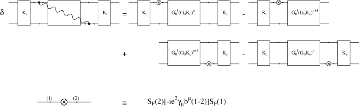
Figure 6: $\delta\left(~{}K_{c}G_{0}I_{n}G_{0}K_{c}\right)=A_{n}G_{0}K_{c}-A_{n+1}+B_{n+1}-K_{c}G_{0}B_{n}$ .

From (3.5) it follows:

$$\delta\sum_{n=1}^{\infty}\langle I_{n}\rangle=\langle A_{1}\rangle-\langle B_{1}\rangle~{},$$ (3.6)

and:

$$\delta\langle\Gamma_{0}\rangle=\langle A_{0}\rangle-\langle A_{1}\rangle+\langle B_{1}\rangle-\langle B_{0}\rangle~{}.$$ (3.7)

It is easy to verify that:

$$\langle A_{0}\rangle = \langle B_{1}\rangle~{},$$ (3.8)

$$\langle B_{0}\rangle = \langle A_{1}\rangle~{},$$ (3.9)

then from (3.6), (3.7) one obtains (3.4).

Similar to the artificial graphs of Fig.5 are the graphs of Fig.7 which effectively contribute to the kernel $K$ of the Bethe-Salpeter equation.

b

Figure 7: $n$ ladder photon crossed by one other.

Since,

$$\langle\Gamma_{1}\rangle^{Fey} = 2\langle I_{1}\rangle^{Fey}+\langle T\rangle^{Fey}+O(\alpha^{4})~{},$$ (3.10)

$$\langle\Gamma_{n}\rangle^{Fey} = \langle I_{n}\rangle^{Fey}+O(\alpha^{4})~{}~{}~{}~{}~{}n>1~{},$$ (3.11)

and up to order $\alpha^{4}$ the Barbieri-Remiddi kernel is local, using the result (3.4), one expects that the spurious terms in (3.1) are cancelled by the ones coming from (3.10) and (3.11). In fact,

$$2\langle I_{1}\rangle^{Fey}_{1S} = {1\over 2\pi}\alpha^{3}\log\alpha-{5\over 2\pi}\alpha^{3}+{4\over\pi}\log 2~{}\alpha^{3}+O(\alpha^{4})~{},$$ (3.12)

$$\sum_{n=2}^{\infty}\langle I_{n}\rangle^{Fey}_{1S} = {9\over 8\pi}\alpha^{3}-{2\over\pi}\log 2~{}\alpha^{3}+O(\alpha^{4})~{}.$$ (3.13)

The sum of (3.12) and (3.13) ($\times 2$ taking in account the symmetric graphs) cancel completely the $\alpha^{3}$ terms in (3.1).

Up to order $\alpha^{3}$ the term $\langle T\rangle^{Fey}$, which comes from $\Gamma_{1}$ subtracting from each photon the zeroth-order kernel $K_{c}$, contributes also to $\langle\Gamma_{1}\rangle^{Fey}$ :

$$\langle T\rangle^{Fey}_{1S}={1\over 2\pi}\log 2~{}\alpha^{3}+O(\alpha^{4})~{}.$$ (3.14)

To obtain the cancellation of (3.14), the graph of Fig.8, arising from the second order perturbations at the energy levels, must be considered; in fact,

$$\left\langle(\Gamma_{0}-K_{c})G_{0}(\Gamma_{0}-K_{c})\right\rangle^{Fey}_{1S}=-{1\over 2\pi}\log 2~{}\alpha^{3}+O(\alpha^{4})~{}.$$ (3.15)

b

Figure 8: $\Gamma_{0}G_{0}\Gamma_{0}$ graph.

References

[1]
S. Love, Ann. Phys. 113 (1978) 153;
G. Feldman, T. Fulton and D. L. Heckathorn, Nucl. Phys. B 167 (1980) 364
and B 174 (1980) 89;
[2]
R. Barbieri and E. Remiddi, Nucl. Phys. B 141 (1978) 413;
[3]
E. Remiddi in these Proceedings;
[4]
W.Buchmüller and E.Remiddi, Nucl. Phys. B 162 (1980) 250.