McGill 96-16

hep-ph/9609240

September 3, 1996

Electroweak Phase Transition
in Two Higgs Doublet Models

James M. Cline

and

Pierre-Anthony Lemieux

McGill University, Montréal, Québec H3A 2T8, Canada

Abstract

We reexamine the strength of the first order phase transition in the electroweak theory supplemented by an extra Higgs doublet. The finite-temperature effective potential, $V_{\rm eff}$, is computed to one-loop order, including the summation of ring diagrams, to study the ratio $\phi_{c}/T_{c}$ of the Higgs field VEV to the critical temperature. We make a number of improvements over previous treatments, including a consistent treatment of Goldstone bosons in $V_{\rm eff}$, an accurate analytic approximation to $V_{\rm eff}$ valid for any mass-to-temperature ratios, and use of the experimentally measured top quark mass. For two-Higgs doublet models, we identify a significant region of parameter space where $\phi_{c}/T_{c}$ is large enough for electroweak baryogenesis, and we argue that this identification should persist even at higher orders in perturbation theory. In the case of the minimal supersymmetric standard model, our results indicate that the extra Higgs bosons have little effect on the strength of the phase transition.

1 Introduction

There is now convincing evidence that the baryon asymmetry of the universe could have been created at the electroweak phase transition (EWPT) [1], with a minimal amount of new, yet plausible physics beyond the standard model [2]-[4]. However for electroweak baryogenesis to work, it is necessary that the baryon-violating interactions induced by electroweak sphalerons be sufficiently slow immediately after the phase transition to avoid the destruction of the baryons that have just been created. This condition is fulfilled if the vacuum expectation value (VEV) of the Higgs field in the broken phase is large enough compared to the critical temperature at the time of the transition (see for example ref. [5] and references therein),

$$\phi_{c}/T_{c}>1.$$ (1)

In the standard model, the bound (1) holds only for very light Higgs bosons [6]-[10] already ruled out by experiment, $m_{h^{0}}<20$ GeV, according to a recent nonperturbative study of the phase transition [11]. In addition to the difficulties with producing a large enough initial baryon asymmetry, the impossibility of satisfying the sphaleron constraint (1) in the standard model provides an incentive for seeing whether the situation improves in extended theories.

The EWPT in two-Higgs doublet models has been previously studied in references [12]-[14]. In the present work we improve on the approximations made in the previous studies in the following ways.

$\bullet$ Avoidance of the unitary gauge, which is known to be problematic: it has been shown that it is necessary to resum an infinite number of contributions in the perturbative expansion to make the determination of finite-temperature quantities agree between unitary gauge and renormalizable gauges [15].

$\bullet$ Inclusion of the ${\mu_{3}^{2}}\Phi_{1}^{\dagger}\Phi_{2}$ term in the Higgs potential necessary for CP violation, which is crucial for the baryon asymmetry production mechanism. In contrast to ref. [14], we find that the strength of the transition does not necessarily grow with increasing ${\mu_{3}^{2}}$.

$\bullet$ Use of the ring summation [6]-[8],[16] for all the bosonic thermal loop contributions to the effective potential. Furthermore we compare two different prescriptions for implementing ring-improvement. The differences are indicative of the theoretical uncertainties inherent in using one-loop perturbation theory.

$\bullet$ Use of a critical temperature $T_{c}$ more closely corresponding to the onset of bubble nucleation, namely the temperature where the two minima of the potential are degenerate, rather than that where the second derivative of the potential vanishes at the origin of field space. We find a quantitative difference between the two methods when determining whether a given set of parameters in the model is really consistent with the sphaleron bound.

$\bullet$ Use of the experimentally measured top quark mass, $175\pm 6$ GeV [17], which was not available when the previous papers [12]-[14] were written. The large mass of the top quark greatly reduces the strength of the phase transition in the standard model [8]-[10].

$\bullet$ Estimating the expansion parameter which quantifies the convergence of the perturbative expansion at the phase transition, near the critical value of the Higgs field VEV[18, 8]. This is the major potential weakness of the perturbative approach being used here. However we find that according to this criterion, most of the promising regions of parameter space are relatively safe from the infrared divergences that would cast doubt on the convergence of the loop expansion.

$\bullet$ Inclusion of the Goldstone boson contributions to the effective potential. These can become important when the lightest Higgs boson $h^{0}$ starts to become as heavy as the other particles in the theory. Although the case of large $m_{h^{0}}$ is uninteresting in the standard model, from the point of view of having a strongly first order phase transition, in extended models the effect of large $m_{h^{0}}$ can be compensated by new particles.

$\bullet$ Avoiding the expansion in mass over temperature that would limit the scope of our investigation. This turns out to be quite important since the region of parameter space where the phase transition is strongly first order is largely where the conventional expansion of the effective potential in powers of $M/T$ is starting to fail badly.

A price we pay for these improvements is the restriction of the potential such that the ratio of the two Higgs VEV’s ($\tan\beta$) is unity, to make the problem more tractable; thus we are not exploring the entire parameter space of the class of models of interest. On the other hand, this reduction has the advantage of making it easier to characterize the favored values of the parameters in the Higgs potential. Furthermore a number of studies of the minimal supersymmetric standard model (MSSM) indicate that the strength of the phase transition is generally greatest for small values of $\tan\beta$ [19]-[24]. In section 4 we discuss the significance of our results for the MSSM in the region of $\tan\beta=1$.

2 Effective Potential

2.1 Zero temperature; Goldstone boson contributions

We begin by constructing the effective potential for the CP-even component of the Higgs field that is responsible for electroweak symmetry breaking. At one loop and at zero temperature, each particle makes a Coleman-Weinberg-type contribution to $V_{{\rm eff},0}(\phi)$ [25]. It can be written in the form of a supertrace involving the matrix $M$ of all the field-dependent particle masses,

$$V_{{\rm eff},0}(\phi)=\frac{\lambda}{4}(\phi^{2}-v^{2})^{2}+\frac{1}{2}A\phi^{2}+\frac{1}{64\pi^{2}}{\rm Str}\,M^{4}(\phi)\left(\log{M^{2}(\phi)\over\mu^{2}}-\frac{3}{2}\right),$$ (2)

where the pieces proportional to $A$ and $\log(\mu^{2})$ are counterterms that must be fixed by renormalization conditions. A convenient choice of the latter is that the tree-level definitions of the VEV ($v=246$ GeV) and the Higgs mass $m^{2}_{h^{0}}=V^{\prime\prime}(v)=2\lambda v^{2}$ should be maintained. These conditions are given by

$$0 =V^{\prime}(v) =Av+\frac{1}{32\pi^{2}}{\rm Str}\,M^{2}{M^{2}}^{\prime}\left(\log{M^{2}\over\mu^{2}}-1\right)$$ (3)

$$m^{2}_{h^{0}} =V^{\prime\prime}(v) =2\lambda v^{2}+A+\frac{1}{32\pi^{2}}{\rm Str}\left[\left(M^{2}{M^{2}}^{\prime\prime}+({M^{2}}^{\prime})^{2}\right)\left(\log{M^{2}\over\mu^{2}}-1\right)+({M^{2}}^{\prime})^{2}\right]$$ (4)

where the prime denotes $\partial/\partial\phi$ and all masses are evaluated at $\phi=v$. One can always choose $A$ such that eq. (4) is satisfied when $m^{2}_{h^{0}}=2\lambda v^{2}$, so the tree-level relation between $m^{2}_{h^{0}}$ and the VEV is preserved.

However there is a technical problem with eq. (4): in the Landau gauge which is the most convenient one because of the decoupling of the ghosts, the Goldstone bosons are massless at $\phi=v$, but they have a nonvanishing value of ${M^{2}}^{\prime}(v)$, giving a logarithmic infrared divergence due to the term $({M^{2}}^{\prime})^{2}\log{M^{2}}$, which does not occur in other gauges. Yet physical masses must be gauge-invariant and IR-finite. The problem is that $m^{2}_{h^{0}}$ as defined in (4) is not the physical pole mass, which must be evaluated at an external momentum of $p^{2}=m^{2}_{h^{0}}$, but rather the off-shell self-energy evaluated at $p^{2}=0$. To avoid the IR divergence and the gauge dependence we should really evaluate the pole mass. By computing the Feynman diagrams of the type shown in figure 1 which are responsible for the IR problem, it is easy to see how to fix it: in eq. (4) one should make the replacement

Figure 1: self-energy diagram responsible for IR-divergent contribution of Goldstone bosons to the Higgs boson mass at $p^{2}=0$, in Landau gauge.

$$\log M^{2} \to {\rm Re}\,\int_{0}^{1}dx\log\left(M^{2}-x(1-x)m^{2}_{h^{0}}\right)$$

$$= \log m^{2}_{h^{0}}-2+\left\{\begin{array}[]{ll}\sum_{\pm}(1\pm\sqrt{1-4R})\log(\frac{1}{2}\pm\sqrt{\frac{1}{4}-R}),&R<\frac{1}{4};\\ \log R+2\sqrt{4R-1}\,\tan^{-1}\left({1\over\sqrt{4R-1}}\right),&R>\frac{1}{4};\end{array}\right.$$

$$\equiv F(M^{2},m^{2}_{h^{0}});\qquad R\equiv M^{2}/m^{2}_{h^{0}},$$

Using the prescription of eqs. (4-2.1), and the convention $m^{2}_{h^{0}}=2\lambda v^{2}$, it is straightforward to solve for the renormalization constants:

$$\log\mu^{2} = {\rm Str}\left[\left({M^{2}}{M^{2}}^{\prime}/v+({M^{2}}^{\prime})^{2}\right)F(M^{2},m^{2}_{h^{0}})-({M^{2}}{M^{2}}^{\prime}/v)\log(M^{2})\right]/{\rm Str}\,({M^{2}}^{\prime})^{2};$$

$$A = -\frac{1}{32\pi^{2}v}{\rm Str}\,M^{2}{M^{2}}^{\prime}\left(\log{M^{2}\over\mu^{2}}-1\right).$$ (8)

We used the fact that for any renormalizable theory, ${M^{2}}^{\prime\prime}={M^{2}}^{\prime}/v$, to simplify the result.

By this procedure we are able to consistently include the contributions of the Goldstone bosons into the effective potential (2). In the standard model, for small values of $m^{2}_{h^{0}}$ which were of interest for maximizing the strength of the phase transition, both the usual Higgs boson and thus the Goldstone bosons make numerically small contributions to the effective potential and can thus be safely ignored. In two Higgs doublet models however, we will show that it is possible to get strong phase transitions even when $m^{2}_{h^{0}}$ becomes rather large, and therefore the Goldstone boson contributions can be nonnegligible.

2.2 Finite temperature

At one-loop order but now at finite temperature, there is an additional contribution to the effective potential given by [26]

$$\Delta V_{{\rm eff},T}(\phi)=\frac{T^{4}}{2\pi^{2}}{\rm Str}\int_{0}^{\infty}dx\,x^{2}\ln\left(1\mp e^{-\sqrt{x^{2}+M^{2}(\phi)/T^{2}}}\right)$$ (9)

where the sign is $-$ for bosons and $+$ for fermions. For small $M/T$ the contribution per degree of freedom can be expanded as

$$V_{\rm s,b}(n)=-\frac{\pi^{2}T^{4}}{90}+\frac{M^{2}T^{2}}{24}-\frac{M^{3}T}{12\pi}-\frac{M^{4}}{64\pi^{2}}\left(\log\left(\frac{M^{2}}{T^{2}}\right)-c_{b}\right)$$ (10)

$$+\frac{M^{2}T^{2}}{2}{\displaystyle\sum^{n}_{l=2}}\left(\frac{-M^{2}}{4\pi^{2}T^{2}}\right)^{l}\frac{(2l-3)!!\zeta(2l-1)}{(2l)!!(l+1)}, {\rm bosons};$$

$$V_{\rm s,f}(n)=-\frac{7\pi^{2}T^{4}}{720}+\frac{M^{2}T^{2}}{48}+\frac{M^{4}}{64\pi^{2}}\left(\log\left(\frac{M^{2}}{T^{2}}\right)-c_{f}\right)$$

$$-\frac{M^{2}T^{2}}{2}{\displaystyle\sum^{n}_{l=2}}\left(\frac{-M^{2}}{4\pi^{2}T^{2}}\right)^{l}\frac{(2l-3)!!\zeta(2l-1)}{(2l)!!(l+1)}\left(2^{2l-1}-1\right), {\rm fermions};$$

$$c_{b}=3/2+2\log 4\pi-2\gamma_{\scriptscriptstyle E}\cong 5.40762;\qquad c_{f}=c_{b}-2\log 4\cong 2.63503$$

where $\zeta$ is the Riemann $\zeta$ function. The term cubic in the boson masses is especially important because it gives rise to the barrier in the potential that makes the transition first order, as needed for baryogenesis. For large $M/T$ on the other hand, the contribution from either bosons or fermions has the asymptotic expansion

$$V_{\rm l}(n)=-e^{-M/T}\left(\frac{MT}{2\pi}\right)^{3/2}\sum_{l=0}^{n}\frac{1}{2^{l}l!}\,\frac{\Gamma(5/2+l)}{\Gamma(5/2-l)}(T/M)^{l}.$$ (11)

For the purpose of numerical analysis of the phase transition, it is useful to have an analytic approximation to the exact expression (9) since it is computationally expensive to evaluate the integral. However, by smoothly joining the small $M/T$ expansion (10) with that for large $M/T$, eq. (11), one can obtain an excellent approximation to the exact integral. To do this optimally, one should choose the value of $M/T$ where the derivatives of the two expansions match each other as the transition point. Using $V_{\rm l}(3)$ for the large $M/T$ approximation, we found good matching to the exact integral by using $V_{\rm s,b}(3)$ for bosons and $V_{\rm s,f}(5)$ for fermions. This gives an approximation with a relative error which is less than 0.5% for $M/T=\infty$, and negligible for small $M/T$. Specifically, we took

$$\Delta V_{{\rm eff},T}={\rm Tr}\Bigl{[} \left[\Theta(x_{b}-(M/T)^{2})\,V_{\rm s,b}(3)+\Theta((M/T)^{2}-x_{b})\,(V_{\rm l}(3)-\delta_{b})\right]P_{b}$$ (12)

$$\left[\Theta(x_{f}-(M/T)^{2})\,V_{\rm s,f}(4)+\Theta((M/T)^{2}-x_{f})\,(V_{\rm l}(3)-\delta_{f})\right]P_{f} {\rm}\Bigr{]},$$

where $\Theta$ is the step function with $x_{b}=9.47134$ and $x_{f}=5.47281$, and $P_{b,f}$ denotes the projection operator for bosons or fermions, respectively. The small constant shifts of $V_{\rm l}(3)$ are made so that the function as well as its derivatives match at the transition point: $\delta_{b}=3.1931\times 10^{-4}$ and $\delta_{f}=4.60156\times 10^{-4}$.

The above discussion implicitly assumed real-valued masses, but for completeness there is one further matching of large and small $M/T$ behavior which must be considered separately: it can happen that some of the bosons have large and negative values of $M^{2}$, corresponding to imaginary $M/T$. While it may be arguable whether eq. (9) has a meaningful physical interpretation for negative $M^{2}$, to the extent that it has any meaning, it is clearly necessary to use the large $M/T$ expansion when $|M^{2}/T^{2}|$ is large. For negative values of $(M/T)^{2}$ the matching conditions are different; in eq. (12) one should use $x_{b}=-6.84368$ and $\delta_{b}=0.045374$. Since large values of $|M^{2}/T^{2}|$ always imply the decoupling of the heavy particles, none of our results concerning the interesting regions of parameter space, where the sphaleron constraint eq. (1) is satisfied, will depend on the precise value of the effective potential when the squared masses are large and negative.

One can easily improve the above one-loop result by resumming a subclass of thermal loops known as the ring diagrams, which amounts to finding the thermal corrections to the boson masses due to $\Delta V_{{\rm eff},T}(\phi)$, typically of the form $M^{2}(\phi,T)=M^{2}(\phi)+g^{2}T^{2}$, and substituting them back into the expression for the total effective potential [16]. In fact the choice of exactly how to resum is not unique, and Arnold and Espinosa [8] have justified the consistency of the widely-used procedure of replacing $M^{2}(\phi)\to M^{2}(\phi,T)$ only in the cubic term $M^{3}T$ of eq. (10) rather than everywhere in the effective potential. Defining the unresummed total one-loop effective potential as

$$V_{\rm tot}=V_{{\rm eff},0}+\Delta V_{{\rm eff},T},$$ (13)

the ring-improved potential in the two methods can be written as

$$V_{\rm ring}=V_{\rm tot}[M^{2}(\phi,T)],$$ Parwani method

$$V_{\rm ring}=V_{\rm tot}[M^{2}(\phi)]+\frac{T}{12\pi}\sum_{\rm bosons}(M^{3}(\phi)-M^{3}(\phi,T)),$$ Arnold-Espinosa method

We shall investigate and compare both of these prescriptions. Since they differ by terms which are of two-loop order, they can give us some idea of the uncertainties in our calculation coming from the neglect of higher orders in perturbation theory.

The ring summation is essential for correctly estimating the contributions from the longitudinal gauge bosons, which get a much larger thermal mass than their transverse counterparts, because this tends to reduce the effectiveness of the cubic term in making the phase transition first order. In addition, the thermal corrections decrease the region of field space near $\phi=0$ where some of the squared masses of the bosons become negative, giving rise to a complex potential. However the imaginary part of the potential can still persist because of the genuine instability of field configurations with small values of $\phi$. We find that the real part of the potential often exhibits an additional local minimum especially when some of the bosons have a small or negative $M^{2}$, as illustrated in figure 2. Such a situation indicates that the negative squared masses of the Higgs bosons are playing a large role and that perturbation theory should not be trusted due to infrared divergences in the effective three dimensional theory which describes the high temperature limit. We discuss the consequences of this phenomenon further below.

Figure 2: Evolution of the effective potential with temperature, showing the pathological case of two nontrivial minima, indicative of negative squared boson masses. The parameter values are $m_{h_{0}}=125$ GeV, ${\mu_{3}^{2}}=(30$ GeV)² and all other Higgs boson masses 187 GeV.

3 Two Higgs Doublet Model

Let us now introduce the new physics. For the two Higgs doublet model, including the couplings to the top quark, the potential is taken to be

$$V_{\rm 2-doublet}(\Phi_{1},\Phi_{2}) = -\mu_{1}^{2}\Phi_{1}^{\dagger}\Phi_{1}-\mu_{2}^{2}\Phi_{2}^{\dagger}\Phi_{2}-{\mu_{3}^{2}}\Phi_{1}^{\dagger}\Phi_{2}-{\mu_{3}^{2}}^{*}\Phi_{2}^{\dagger}\Phi_{1}+\frac{\lambda_{1}}{2}(\Phi_{1}^{\dagger}\Phi_{1})^{2}+\frac{\lambda_{2}}{2}(\Phi_{2}^{\dagger}\Phi_{2})^{2}$$ (14)

$$+ h_{1}(\Phi_{1}^{\dagger}\Phi_{2})(\Phi_{2}^{\dagger}\Phi_{1})+h_{2}(\Phi_{1}^{\dagger}\Phi_{1})(\Phi_{2}^{\dagger}\Phi_{2})+h_{3}\left((\Phi_{1}^{\dagger}\Phi_{2})^{2}+(\Phi_{2}^{\dagger}\Phi_{1})^{2})\right)$$

$$+ \overline{T}_{\scriptscriptstyle L}(y_{1}\Phi_{1}+y_{2}\Phi_{2})t_{\scriptscriptstyle R}+{\rm\ c.c.}$$

It incorporates a softly-broken discrete symmetry, $\Phi_{i}\to-\Phi_{i}$, in order to reduce the number of possible couplings. This is the same model as discussed in ref. [13], except for the addition of the term ${\mu_{3}^{2}}\Phi_{1}^{\dagger}\Phi_{2}$, which is necessary for having CP violation in the Higgs sector. To simplify the analysis, we follow ref. [13] by setting $\mu_{1}^{2}=\mu_{2}^{2}$, $\lambda_{1}=\lambda_{2}$ and $y_{1}=y_{2}$. Furthermore we assume that ${\mu_{3}^{2}}$ is real and positive. This choice insures that the symmetry will break along the direction $\Phi_{1}=\Phi_{2}\equiv\frac{1}{2}(0,\phi)^{\scriptscriptstyle T}$ at any temperature. The resulting potential for $\phi$ is identical to the standard form $\lambda(\phi^{2}-v^{2})^{2}/4$ used in (2) if one identifies

$$\lambda=\frac{1}{4}(\lambda_{1}+h_{1}+h_{2}+2h_{3});\qquad v^{2}=\frac{\mu^{2}_{1}+{\mu_{3}^{2}}}{\lambda}.$$ (15)

The spectrum consists of the light Higgs boson $h^{0}$ associated with the field $\phi$, three Goldstone bosons $G^{0},G^{\pm}$, the charged particles $H^{\pm}$, and the neutral scalar and pseudoscalar, $H^{0}$ and $A^{0}$ repsectively.

All that remains to complete the definition of the effective potential is to specify the field- and temperature-dependent masses. For the gauge bosons these are the eigenvalues of the mass matrix in the basis $W^{\pm}$, $W^{3}$, $B$,

$$m^{2}_{\rm gauge}(\phi,T)={\phi^{2}\over 4}\left(\begin{array}[]{cccc}g^{2}&&&\\ &g^{2}&&\\ &&g^{2}&gg^{\prime}\\ &&gg^{\prime}&g^{\prime 2}\end{array}\right)+T^{2}\left(\begin{array}[]{cccc}g^{2}&&&\\ &g^{2}&&\\ &&g^{2}&\\ &&&g^{\prime 2}\end{array}\right)\left\{\begin{array}[]{rl}2,&{\rm longitudinal;}\\ 0,&{\rm transverse.}\end{array}\right.$$ (16)

Notice that only the longitudinal gauge bosons get a thermal mass at this order (for the transverse bosons there is a magnetic mass of order $g^{2}T$ which we neglect) and the coefficient $2$ in the thermal correction would be $11/6$ in the absence of the second Higgs doublet. Also the longitudinal photon is no longer massless at finite temperature, due to mixing between $B$ and $W^{3}$. The top quark mass is

$$m_{t}(\phi,T)=m_{t}{\phi\over v}.$$ (17)

Although the dispersion relation for the top quark does get temperature corrections which can be interpreted as a thermal contribution to its mass squared, these do not appear in the resummation of the ring diagrams because it is a fermion, as explained above. For the Higgs bosons, it is convenient to eliminate all the dimensionless couplings and express the general masses in terms of the zero-temperature ones and the parameter ${\mu_{3}^{2}}$ [4]:

$$m^{2}_{i}(\phi,T) = \left\{\begin{array}[]{ll}\frac{1}{2}\left(-m^{2}_{h^{0}}+(m^{2}_{h^{0}}+2m^{2}_{i}){\phi^{2}\over v^{2}}\right)+\left(a+{y_{1}y_{2}\over 4}\right)T^{2},&i=h^{0},G^{0},G^{\pm};\\ \frac{1}{2}\left(-m^{2}_{h^{0}}+4{\mu_{3}^{2}}+(m^{2}_{h^{0}}-4{\mu_{3}^{2}}+2m^{2}_{i}){\phi^{2}\over v^{2}}\right)+\left(a-{y_{1}y_{2}\over 4}\right)T^{2},&i=A^{0},H^{0},H^{\pm};\end{array}\right.$$ (20)

$$a = {\lambda\over 2}+\frac{3g^{2}+g^{\prime 2}}{16}+\frac{y_{1}^{2}+y_{2}^{2}}{8}+\frac{1}{12}\left\{4\lambda+{1\over v^{2}}(-8{\mu_{3}^{2}}+2m^{2}_{H^{\pm}}+m^{2}_{H^{0}}+m^{2}_{A^{0}})\right\};$$

For comparison, the standard model can be recovered by ignoring the masses of $A^{0},H^{0},H^{\pm}$ and the term in curly brackets in $a$, and setting $y_{2}=0$. The particle multiplicities are 1 for each of the Higgs bosons and the longitudinal gauge bosons, 2 for each transverse gauge boson, and 12 for the top quark.

4 Phase Transition Results

In studying the quantity $\phi_{c}/T_{c}$ one should in principal take care to distinguish between various definitions of the critical temperature. The $T_{c}$ relevant for baryogenesis is the temperature when tunneling from the false vacuum to the true vacuum takes place, after which the phase transition quickly completes. To determine it precisely, one demands that the tunneling probability becomes sufficiently large compared to the Hubble expansion rate, which requires solving for the bubble configurations and computing their action [10]. In the standard model, rather close upper and lower bounds on $T_{c}$ can be obtained because it is always above the temperature $T_{0}$ where $V^{\prime\prime}(0,T_{0})=0$, and below the temperature $T_{1}$ when the nontrivial minimum $v(T)$ in the potential becomes degenerate with the minimum at the origin, and these temperatures are all within a few tenths of a percent of each other. However in extended models it might be important to make the distinction between the various critical temperatures because they can differ more substantially, and also because $v(T)/T$ can change rather quickly near the critical temperature. In the following we compare the results of using either definition of the critical temperature and find some noticeable differences, particularly for small values of the Higgs mass parameter ${\mu_{3}^{2}}$.

Because the masses of the heavy Higgs bosons ($A^{0}$, $H^{0}$ and $H^{\pm}$) have such a similar form in eq. (LABEL:Higgsmasses), we have simplified our scan of the parameter space by taking them all to be equal to each other. Figure 3 shows the contours of constant $\phi/T$ in the plane of $m_{A^{0}}=m_{H^{0}}=m_{H^{\pm}}$ versus $m_{h^{0}}$, using three different methods. The first column uses $T_{0}$ as the definition of the critical temperature, and the Arnold-Espinosa method of ring-improvement. The second column is the same except using $T_{1}$ for the critical temperature. The third column also uses $T_{1}$, but the Parwani ring-improvement prescription. Each row is for a separate value of the potential parameter ${\mu_{3}^{2}}$, ranging between 0 and $6\times 10^{4}$ GeV².

                 $T_{0}$                    Arnold-Espinosa               Parwani                         $\epsilon$ $m_{A^{0},H^{0},H^{\pm}}\!\!\uparrow$ ${\mu_{3}^{2}}=0$ ${\mu_{3}^{2}}=3$ ${\mu_{3}^{2}}=6$      $m_{h^{0}}\rightarrow$

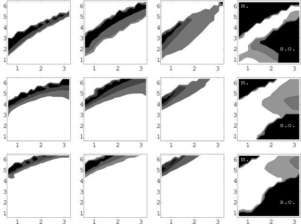
Figure 3: Contours of constant $\phi_{c}/T_{c}$ (first three columns) and the perturbative expansion parameter $\epsilon$ (defined in eq. (24)) for three values of ${\mu_{3}^{2}}$, in the plane of $m_{A^{0}}=m_{H^{0}}=m_{H^{\pm}}$ versus $m_{h^{0}}$. The first three columns use different approximations for the critical temperature or the effective potential, described in the text. Units are 100 GeV for masses, (100 GeV)² for ${\mu_{3}^{2}}$. Increasing values are represented by darker shades, with white being $<1$ and increasing in steps of $1$. The regions labeled by “m.” in the last column are where the false vacuum is metastable, and those labeled “s.o.” are where the phase transition is second order, as illustrated in figure 4. In neither case is there a first order transition. The values of $\epsilon$ are computed using the boson masses corresponding to the second column.

The regions in white are those with $\phi_{c}/T_{c}<1$, and therefore indicate the parameters for which electroweak baryogenesis would not work in this model. In all three methods one sees that for a given value of $m_{h^{0}}$, there exists a range of the other masses such that $\phi_{c}/T_{c}>1$. When the other masses are greater than this range, it turns out that the nontrivial minimum is higher than the one at $\phi=0$ even at zero temperature, meaning that the electroweak symmetry breaking vacuum is metastable and there is no phase transition, unless supercooling into the metastable minimum occurs. On the other hand, when they lie below the allowed bands, the transition becomes second order, because there is never any barrier separating the minimum at $\phi=0$ from the symmetry-breaking minimum. In either case we define $\phi_{c}/T_{c}$ to be zero. Such examples are illustrated in figure 4.

Figure 4: Examples of the evolution of the potential with temperature which illustrate the absence of a first order phase transition. In the first one the false vacuum is metastable, and in the second the phase transition is second order. The parameter values are $m_{h^{0}}=60$ GeV, other masses $=325$ GeV, ${\mu_{3}^{2}}=0$ for the first one, and $m_{h^{0}}=300$ GeV, other masses $=250$ GeV, ${\mu_{3}^{2}}=0$ for the second.

However the three methods of constructing the finite-temperature potential differ as to the precise values of $\phi_{c}/T_{c}$ when ${\mu_{3}^{2}}$ is small, with the Parwani ring-improvement giving larger values than that of Arnold and Espinosa. For large ${\mu_{3}^{2}}$, all three give similar results. Where the two methods of resummation differ is indicative of where perturbation theory may be unreliable. There is another curious phenomenon for small but nonzero values of ${\mu_{3}^{2}}$, for example ${\mu_{3}^{2}}=(30$ GeV)², which is not shown in figure 3: the region allowed by baryogenesis appears to be significantly enlarged in the first two methods ($T_{0}$ and Arnold-Espinosa), though not in the third. Examination of the potential shows that the region of enlargement is always accompanied by the existence of double minima, as in figure 2. Therefore the augmentation of the baryogenesis-allowed parameter space in these cases is spurious. This is one possible explanation for our failure to corroborate the claim of ref. [14], which says that increasing ${\mu_{3}^{2}}$ generally has a favorable effect on the strength of the phase transition.

In addition to comparing different methods of ring-improvement, we can also quantify the convergence of the perturbative expansion in an independent way, by trying to estimate what is the true expansion parameter for the finite-temperature theory, near the critical value of $\phi$. Let us first review how the perturbative power counting argument goes in the standard model. The cost of adding one additional thermal loop of $W$ bosons to an arbitrary Feynman diagram contributing to the free energy is

$${g^{2}T_{c}\over(2\pi)^{3}}\int{d^{3}p\over(p^{2}+m^{2}_{W}(\phi_{c}))^{2}}\propto{g^{2}T_{c}\over m_{W}(\phi_{c})}={6\pi\,m_{W}\,m^{2}_{h^{0}}\over 2m^{3}_{W}+m^{3}_{Z}}\cong\left({m_{h^{0}}\over 35{\rm\ GeV}}\right)^{2},$$ (22)

where we used $m_{W}(\phi_{c})=g\phi_{c}/2$, $m^{2}_{h^{0}}=2\lambda_{\rm eff}v^{2}$, and the standard model value for critical ratio $\phi_{c}/T_{c}\cong\phi_{0}/T_{0}=(2m^{3}_{W}+m^{3}_{Z})/(2\pi\lambda v^{3})$. In ref. [11] it was shown that the true loop expansion parameter is around $0.4$ for a Higgs mass of 35 GeV, while ref. [8] finds that $\phi_{c}/T_{c}$ changes by 30% in going from one loop to two loops when $m_{h^{0}}$ is near 35 GeV. In a two-Higgs doublet model, it is no longer the $W$ boson which gives the dominant corrections to the potential, but rather the new Higgs bosons. Thus the expansion parameter will be $\lambda_{i}T_{c}/m^{2}_{i}(\phi_{c})$ instead of (22), where $\lambda_{i}$ and $m_{i}$ are any of the quartic couplings and corresponding mass eigenvalues, respectively, of the new Higgs sector. The couplings of the mass eigenstates will be linear combinations of the couplings in the Lagrangian, $\lambda_{1}$, $h_{1}$, $h_{2}$ and $h_{3}$, which are given by eq. (15) and the relations [4]

$$h_{1} = 2\lambda(2{\mu_{3}^{2}}-2m^{2}_{\pm}+m^{2}_{A^{0}})/m^{2}_{h^{0}};$$

$$h_{2} = 2\lambda(m^{2}_{h^{0}}-2{\mu_{3}^{2}}+2m^{2}_{\pm}-m^{2}_{H^{0}})/m^{2}_{h^{0}};$$

$$h_{3} = \lambda(2{\mu_{3}^{2}}-m^{2}_{A^{0}})/m^{2}_{h^{0}}.$$ (23)

Comparing with the standard model, it thus seems reasonable and conservative to require that

$$\epsilon\equiv{\max(\lambda_{1},h_{i})T_{c}\over\min(|m_{i}(\phi_{c})|)}\mbox{\raisebox{-2.58334pt}{~{}$\stackrel{{\scriptstyle<}}{{\sim}}$~{}}}1$$ (24)

in order to have some confidence that the perturbative expansion is not out of control due to the infrared problem. In the last column of figure 3 we show the contours of $\epsilon$, using as inputs the thermal masses at $\phi_{c}$ and $T_{c}$ corresponding to the third column. It is interesting to see that $\epsilon$ and $\phi_{c}/T_{c}$ tend to be anticorrelated: where one is big the other is small. This is good news as concerns the trustworthiness of the interesting regions where $\phi_{c}/T_{c}>1$; it means we expect the value of $\phi_{c}/T_{c}$ predicted by the 1-loop result to be rather stable against changes due to higher order contributions.

4.1 Supersymmetry

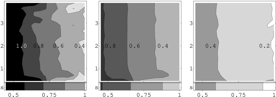
Figure 5: Contours of $\phi_{c}/T_{c}$ in the plane of $m_{A^{0}}$ versus $m_{h^{0}}$, using the same three respective methods as in figure 3, setting the other Higgs boson masses to their tree-level values in the minimal supersymmetric standard model. The horizontal strip at the bottom, labeled “s,” shows the corresponding values in the standard model.

The model we chose to study is not quite a realistic limit of the minimal supersymmetric standard model (MSSM), even in the case that all the superpartners are much heavier than the Higgs bosons and therefore decouple. This is because to be consistent with the assumption that the symmetry breaks in the direction where the two Higgs fields have equal VEV’s, we assumed that the top quark coupled equally to each, which is not possible in supersymmetry. Nevertheless one might trust the model to give a qualitative indication of the effects of the additional Higgs bosons on the phase transition. In the limit of $\tan\beta=1$ to which we restricted ourselves in this study, the tree-level masses of the Higgs bosons are related according to [27]

$$m^{2}_{h^{0}}=0;\quad m^{2}_{H^{0}}=m^{2}_{A^{0}}+m^{2}_{Z};\quad m^{2}_{H^{\pm}}=m^{2}_{A^{0}}+m^{2}_{W},$$ (25)

and the parameter ${\mu_{3}^{2}}=m^{2}_{A^{0}}/2$, as can be seen from eq. (23) using the fact that $h_{3}=0$ in supersymmetry. Of course the $h^{0}$ boson is not really massless, but it gets a mass from loop corrections involving the top squarks, of order $\alpha(m^{2}_{t}/m_{Z})\ln(\tilde{m}_{t}/m_{t})$. Thus we are only interested in rather light $h^{0}$ particles. For the heavier Higgs bosons on the other hand, the tree level relations should be a good approximation for their masses, showing that $m_{A^{0}}$ is the only free parameter.

In figure 5 we display the contours of $\phi_{c}/T_{c}$ using the same three methods as in figure 3, in the plane of $m_{A^{0}}$ versus $m_{h^{0}}$. For comparison, the standard model results are shown in the horizontal strip at the bottom of each graph. In contrast to figure 3, here we see that the distinction between the more accurate critical temperature and the naive one, $T_{0}$, is quite important, and furthermore the differences between the two methods of ring-improvement are significant. The latter observation, comparison with the standard model results, and the lack of variation of $\phi_{c}/T_{c}$ with $m_{A^{0}}$ show that the extra Higgs bosons are generally playing a small role; it is the transverse gauge bosons which are most important in determining the strength of the phase transition. The perturbative expansion parameter corresponding to their contributions, eq. (22), is large for $m_{h^{0}}>35$ GeV, hence the discrepancy between the two methods of resummation. Although there is a hint that very light masses for the extra Higgs bosons can strengthen the phase transition, the apparent instability of the perturbation series in this region renders any such conclusion uncertain.

It is interesting to compare the MSSM case to that shown in figure 3. In the latter one sees that for a fixed value of ${\mu_{3}^{2}}$ it is always possible to choose the other masses large enough to make $\phi_{c}/T_{c}>1$. But in the MSSM, there is a special relation between ${\mu_{3}^{2}}$ and the new Higgs boson masses which prevents them from enhancing the first order nature of the phase transition in the minimal supersymmetric standard model, even when the bosons become quite heavy. This is easily understood in terms of the couplings $h_{i}$ in eq. (23), which are constrained to be of order $g^{2}$ in supersymmetry, whereas in a generic two Higgs doublet model they become large as the scalar masses increase.

Also interesting is the large difference between using the naive critical temperature $T_{0}$ and the more accurate one $T_{1}$. The former gives a substantial overestimate of the strength of the phase transition. In ref. [14], regions of parameter space consistent with $\phi_{c}/T_{c}>1$ were found in the MSSM with $\tan\beta=1$, however using $T_{0}$ as the critical temperature. Our results indicate that one should use a more precise definition of $T_{c}$ before concluding that the Higgs bosons can have much effect on the phase transition.

5 Conclusions

We have investigated the electroweak phase transition in a class of models containing two Higgs doublets, with a global symmetry that insures electroweak symmetry breaking along the direction $\Phi_{1}=\Phi_{2}$. The results are encouraging from the standpoint of electroweak baryogenesis, which requires that $\phi_{c}/T_{c}>1$ to avoid the washout by sphalerons of the baryons that might be produced. Even for rather heavy $h^{0}$ Higgs particles up to 300 GeV, it appears possible to choose the others sufficiently heavy to make a strongly first order transition, except perhaps when the parameter ${\mu_{3}^{2}}$ from the mass term ${\mu_{3}^{2}}\Phi_{1}^{\dagger}\Phi_{2}$ becomes too large. In supersymmetric models however, ${\mu_{3}^{2}}$ is automatically tuned in such a way as to minimize the impact of the extra bosons on the strength of the phase transition, no matter how heavy they are.

We tried to make our study as reliable as possible by using certain improvements: inclusion of Goldstone boson contributions, going beyond the small $M/T$ expansion, and estimating the size of higher order perturbative effects by comparing different methods of ring diagram resummation and by computing the expansion parameter of the finite temperature theory. The latter checks give us confidence that our conclusions are quantitatively correct. However it is always possible that perturbation theory fails despite such safeguards. Recently it has become possible to start investigating the electroweak phase transition in theories with new physics using nonperturbative lattice results, by mapping the theory of interest onto an effective lagrangian of the same light degrees of freedom as in the standard model [28], which has already been analyzed on the lattice. Steps in this direction were recently taken for two Higgs doublet models by reference [29]. It will be interesting to compare the nonperturbative approach with that pursued here, to verify more conclusively that there really are conditions when perturbation theory, which is easier to apply and more amenable to analytic expressions, can be trusted to give quantitatively accurate results for the finite temperature effective potential.

References

-
[1]
M.E. Shaposhnikov, JETP Lett. 44, 465 (1986);
Nucl. Phys. B287, 757 (1987); Nucl. Phys. B299,
797 (1988);
G. Farrar and M. Shaposnikov, Phys. Rev. Lett. 70, 2833 (1993); erratum ibid 71 210 (1993); Phys. Rev. D50, 774 (1993);
M.B. Gavela, P. Hernandez, J. Orloff and O. Pene, Mod. Phys. Lett. A9, 795, (1994), Nucl. Phys. B430, 345 (1994). - [2] A.E. Nelson, D.B. Kaplan and A.G. Cohen, Nucl. Phys. B373, 453 (1991);
- [3] M. Joyce, T. Prokopec and N. Turok, Phys. Lett. B338, 269 (1994); Phys. Rev. Lett. 75,1695 (1995), ERRATUM-ibid. 75, 3375 (1995); Phys. Rev. D53, 2930 (1996); Phys. Rev. D53, 2958 (1996).
- [4] J. Cline, K. Kainulainen and A. Vischer, Phys. Rev. D (to appear)
-
[5]
A. Cohen, D. Kaplan, and A. Nelson, Annual
Review of Nuclear and Particle Science 43, 27 (1994);
V.A. Rubakov and M.E. Shaposhnikov, CERN-TH/96-13, hep-ph 9603208. - [6] M.E. Carrington, Phys. Rev. D45 2933 (1992).
- [7] P. Arnold, Phys. Rev. D46 2628 (1992).
- [8] P. Arnold and O. Espinosa, Phys. Rev. D47, 3546 (1993).
- [9] G.W. Anderson and L.J. Hall, Phys. Rev. D45, 2685 (1992).
- [10] M. Dine, R.G. Leigh, P. Huet, A. Linde and D. Linde, Phys. Rev. D46, 550 (1992).
- [11] K. Kajantie, M. Laine, K. Rummukainen and M.E. Shaposnikov, preprint, CERN-TH/95-263, hep-lat 9510020.
- [12] A.I. Bochkarev, S.V. Kuzmin and M.E. Shaposhnikov, Phys. Lett. B244, 275 (1990).
- [13] N. Turok and J. Zadrozny, Nucl. Phys. B369, 792 (1992);
- [14] A.T. Davies, C.D. Froggatt, G. Jenkins and R.G. Moorhouse, Phys. Lett. B336, 464 (1994).
- [15] P. Arnold, E. Braaten and S. Vokos, Phys. Rev. D46, 3576 (1992).
- [16] R. Parwani, Phys. Rev. D45, 4695 (1992).
- [17] P. Tipton, plenary talk at International Conference on High Energy Physics, 25-31 July 1996, Warsaw, Poland.
- [18] S. Weinberg, Phys. Rev. D9, 2257 (1974).
- [19] J.R. Espinosa, M. Quiros and F. Zwirner, Phys. Lett. B307, 106 (1993).
- [20] A. Brignole, J.R. Espinosa, M. Quiros and F. Zwirner, Phys. Lett. B324, 181 (1994).
- [21] M. Carena, M. Quiros and C.E.M. Wagner, Phys. Lett. B380, 81 (1996).
- [22] J.R. Espinosa, preprint DESY-96-064, hep-ph/9604320 (1996).
- [23] J.M. Cline and K. Kainlulainen, preprint McGill-96-20, hep-ph/9605235, to appear in Nucl. Phys. B (1996).
- [24] M. Laine, preprint HD-THEP-96-13, hep-ph/9605283 (1996).
- [25] S. Coleman and E. Weinberg, Phys. Rev. D7, 1888 (1973).
- [26] L. Dolan and R. Jackiw, Phys. Rev. D9, 3320 (1974).
- [27] see for example J.F. Gunion, H.E. Haber, G.L. Kane and S. Dawson, The Higgs Hunter’s Guide, Addison-Wesley, 1990.
- [28] K. Kajantie, M. Laine, K. Rummukainen and M. Shaposhnikov, Nucl. Phys. B458, 90 (1996).
- [29] M. Losada, Rutgers preprint RU-96-25, hep-ph/9605266 (1996).