Abstract

An improved effective vector-boson approximation is applied to hadron-hadron collisions. I include an approximative treatment and compare with a complete perturbative calculation for the specific example of $ZZ$ production. The results are also compared with existing approaches. The effective vector-boson approximation in this form is accurate enough to reproduce the complete calculation within 10%. This is true even far away from a possible Higgs boson resonance where the transverse intermediate vector-bosons give the dominant contribution.

1 Introduction

The effective photon approximation (EPA) (Weizsäcker-Williams-approximation) of QED [1] has proved to be a useful tool in the study of photon-photon processes at $e^{+}e^{-}$ colliders. With the prospect of high-energy hadron-hadron colliders, the possibility to study the scattering of massive vector-bosons is given. Massive vector-boson scattering is of particular interest as the symmetry breaking sector of the electroweak theory and the self-interactions of the vector-bosons are directly tested. The method equivalent to the EPA applying to the scattering of massive vector-bosons is the effective vector-boson approximation (EVBA) [2, 3, 4, 5]. The EVBA can be applied to fermion-fermion scattering processes in which the final state consists of two fermions and a state $\Xi$ which can be produced by the scattering of two vector-bosons. The fermion-fermion cross-section is written as a product of a probability distribution and the cross-sections for vector-boson scattering. The probability distribution describes the emission of vector-bosons from fermions. The method is an approximate one which neglects Feynman diagrams of bremsstrahlung-type. In general, the method is applicable if the fermion scattering energy is large against the masses of the electroweak vector-bosons.

The possibility of an EVBA has been first noticed in connection with heavy Higgs boson production [6]. The Higgs boson can be produced via the diagram in Figure 1a, where a sum over all vector-boson pairs $V_{1},V_{2}$ which can couple to the Higgs boson is to be taken.

Figure 1: a: The diagram for Higgs boson production in quark-quark scattering, $q_{1}q_{2}\to q^{\prime}_{1}q^{\prime}_{2}H$. b: The diagram for the production of a vector-boson pair $V_{3}V_{4}$ as the decay products of a heavy Higgs boson in $q_{1}q_{2}$ scattering.

In this early application of the EVBA only the contribution from longitudinally polarized intermediate vector-bosons, $V_{1,L}V_{2,L}$, was calculated and the result was found to give a reasonable approximation to an exact perturbative calculation [7].

Subsequently, the EVBA was also applied to processes of the type $pp\to V_{3}V_{4}+X$, where two vector-bosons are produced. The vector-bosons $V_{3}$ and $V_{4}$ emerge as the decay products of a near-resonant heavy Higgs particle [2]. The scattering process was described by the diagram in Figure 1b. Also in this case, the inclusion of only longitudinal intermediate vector-bosons was sufficient. It was noted that the production of heavy particles (Higgs bosons or fermions) is mainly due to the longitudinal intermediate states [4].

The concept of vector-bosons as partons in quarks was further established and expressions for vector-boson distributions in quarks were derived [3, 4]. The expressions were given for all polarizations of the intermediate vector-bosons. By convolution with the quark distributions in a proton, numerical results were given for vector-boson distributions in a proton [3]. For the production via two intermediate vector-bosons it was assumed that convolutions of the distributions of single vector-bosons could describe the emission probability of the vector-boson pair. The EVBA in this form gave reliable results for heavy Higgs boson production [3, 4, 7, 8, 9] and heavy fermion production [10].

The necessity to include all vector-boson scattering diagrams for $V_{1}V_{2}\to V_{3}V_{4}$ in order to obtain EVBA predictions for the production of a vector-boson pair $V_{3}V_{4}$, not necessarily near a Higgs boson resonance, has been first mentioned in [9] and [11]. The possible diagrams for these processes, $q_{1}q_{2}\to q^{\prime}_{1}q^{\prime}_{2}V_{3}V_{4}$, where $q_{i},q^{\prime}_{i}$ are quarks, are shown in Figure 2.

Figure 2: The diagram for $q_{1}q_{2}\to q^{\prime}_{1}q^{\prime}_{2}V_{3}V_{4}$ in the effective vector-boson approximation and the diagrams for vector-boson scattering.

It was further pointed out that the yield of $V_{3}V_{4}$ pairs from $q_{1}q_{2}\to q^{\prime}_{1}q^{\prime}_{2}V_{3}V_{4}$ must be discussed together with the yield from the direct reaction $q_{1}q_{2}\to V_{3}V_{4}$ (Drell-Yan reaction) unless a suitable analysis of the different proton remnants from the two production mechanisms allows to separate the different production mechanisms.

In first applications to vector-boson scattering, again only the contribution from the longitudinal intermediate states was considered while the contribution from transverse states was neglected. This contribution was taken to be small against the $q_{1}q_{2}\to V_{3}V_{4}$ contribution while the contribution from $V_{1,L}V_{2,L}\to V_{3}V_{4}$ could be large if the longitudinal vector-bosons interact strongly. The interest in the strongly interacting scenario [12] was the original motivation to use the EVBA.

The EVBA has been used for vector-boson scattering in [2], [13]-[17]. In [14], the EVBA has been used only for the longitudinal intermediate states. The transverse states have been taken into account by a complete perturbative calculation (to lowest order in the coupling) of the process $q_{1}q_{2}\to q^{\prime}_{1}q^{\prime}_{2}V_{3}V_{4}$. This calculation requires the evaluation of more diagrams than only the vector-boson scattering diagrams, as indicated in Figure 3.

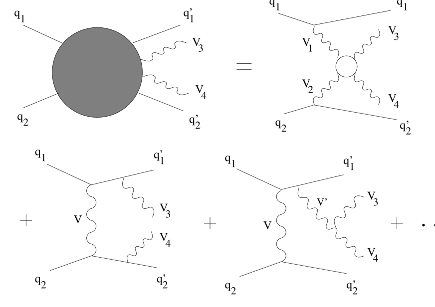
Figure 3: Some of the Feynman diagrams for a process $q_{1}q_{2}\to q^{\prime}_{1}q^{\prime}_{2}V_{3}V_{4}$ in a complete perturbative calculation. In the top row to the right is the diagram for vector-boson scattering, which is the only type of diagram which is considered in the effective vector-boson approximation. The bottom row shows diagrams of bremsstrahlung-type.

To be precise, in [14] the EVBA has been used only to calculate the difference between the cross-sections in a strongly interacting model and in the standard model with a light Higgs boson. This difference shows an interesting behavior in a strongly-interacting scenario and was therefore considered as a potential signal for strongly interacting vector-bosons. The difference receives a contribution virtually only from the longitudinal states. It was found [14] that this calculation agrees with a complete perturbative calculation to about 10% (evidenced for $W^{\pm}Z$ and $W^{\pm}W^{\pm}$ production) if the standard model with a heavy Higgs boson is taken as the strongly-interacting model. I note that for strong scattering a method has been recently described which does not make use of the EVBA [18].

In [13, 16, 17] the application of the EVBA was extended to the contributions from all intermediate polarization states. It was known, however, that the EVBA can overestimate results of complete perturbative calculations by a factor of 3 if the transverse helicities are important [27, 28]. Other comparisons of results of complete calculations for $pp\to V_{3}V_{4}+X$ with EVBA results [24, 25] showed that the EVBA is always a good approximation on the Higgs boson resonance but in general overestimates the transverse contribution which is the important one for vector-boson scattering away from a Higgs boson resonance. The EVBA was found to be unreliable away from the Higgs boson resonance. Furthermore, the EVBA result depends strongly on the details of the approximations made in deriving the EVBA [27, 28]. In particular, the frequently used leading logarithmic approximation can overestimate the transverse luminosity by an order of magnitude [21, 22].

We will obtain exact luminosities $\cal L$ for vector-boson pairs in a hadron pair from an improved formulation of the EVBA, previously introduced for fermion-fermion scattering in [19]. This formulation makes no approximation in the integration over the phase space of the two intermediate vector bosons. The only remaining assumption, necessary in an EVBA, concerns the off-shell behavior of vector-boson cross-sections. The formulation, however, involves multiple numerical integrals and is thus not very practical in itself. However, the exact luminosities $\cal L$ form a unique basis to derive well-defined approximations which turn out to be good. They also serve as a testing ground against which existing formulations of the EVBA can be examined.

In Section 2 the improved EVBA is applied to hadron collisions and numerical results for the exact luminosities are given. We derive useful approximations to the improved EVBA. A comparison with previous formulations of the EVBA is given. Section 3 contains a comparison of EVBA results with a complete perturbative calculation for $pp\to ZZ+X$. Details of various existing formulations of the EVBA are discussed in Appendix A.

2 Luminosities for Vector-Boson Pairs in Hadron Pairs

2.1 Improved Effective Vector-Boson Approximation

Applying the treatment of the improved EVBA [19], we present exact luminosities for finding a vector-boson pair in a hadron-pair. The luminosities apply to the process shown in Figure 4.

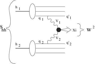
Figure 4: The diagram for the hadron-hadron scattering process proceeding via two intermediate vector-bosons, $h_{1}h_{2}\to q_{1}q_{2}\to q^{\prime}_{1}q^{\prime}_{2}V_{1}V_{2}$ and $V_{1}V_{2}\to\Xi$.

The cross-section for a scattering-process of two hadrons, $h_{1}$ and $h_{2}$, with high energies, in which an arbitrary final state $\Xi$ is produced, is given (in the quark-parton model) by a two-dimensional integral over a product of parton distribution-functions and the cross-section for parton-parton scattering processes,

$$\sigma(h_{1}h_{2}\to\Xi+X,s_{hh})=\sum_{q_{1},q_{2}}\int\limits_{0}^{1}d\xi_{1}\int\limits_{0}^{1}d\xi_{2}f_{q_{1}}^{h_{1}}(\xi_{1},\mu_{1}^{2})f_{q_{2}}^{h_{2}}(\xi_{2},\mu_{2}^{2})\sigma(q_{1}q_{2}\to\Xi+X^{\prime},s_{qq}).$$ (1)

The sum in (1) extends over all partons (quarks, antiquarks and gluons) $q_{1}$ in the hadron $h_{1}$ and $q_{2}$ in the hadron $h_{2}$. The variable $\xi_{i}$ in (1) is the ratio of the momentum of the parton $q_{i}$ and the hadron $h_{i}$. The quantities $f_{q_{i}}^{h_{i}}(\xi_{i},\mu_{i}^{2})$ are the parton distribution functions, evaluated at the momentum fractions $\xi_{i}$ and the factorization scales $\mu_{i}^{2}$. The scale is a characteristic energy of the process which is initiated by the parton $q_{i}$. The quantities $\sigma(q_{1}q_{2}\to\Xi+X^{\prime})$ in (1) are the cross-sections for the parton-parton processes. In (1), $s_{hh}$ is the square of the hadron-hadron scatterig energy, related to the parton-parton scattering energy, $\sqrt{s_{qq}}$, by

$$s_{qq}=\xi_{1}\xi_{2}s_{hh}.$$ (2)

The symbols $X$ and $X^{\prime}$ represent additional particles in the final state. In writing down (1), we assumed that the partons have no transverse momentum. We also neglected the masses of the hadrons and partons. These approximations may be made in any frame in which both hadrons are highly relativistic.

Expressed in terms of the ratio of the squared invariant masses, $\tau\equiv s_{qq}/s_{hh}$, and the rapidity $y_{q}$ of the motion of the center-of-mass of the parton-pair in the center-of-mass system (cms) of the hadrons the cross-section (1) takes on the form

$$\sigma(h_{1}h_{2}\to\Xi+X,s_{hh}) = \sum_{q_{1},q_{2}}\int\limits_{0}^{1}d\tau\int\limits_{\frac{1}{2}\ln(\tau)}^{-\frac{1}{2}\ln(\tau)}dy_{q}\,f_{q_{1}}^{h_{1}}\left(\sqrt{\tau}e^{y_{q}},\mu_{1}^{2}\right)f_{q_{2}}^{h_{2}}\left(\sqrt{\tau}e^{-y_{q}},\mu_{2}^{2}\right)$$ (4)

$$\cdot\sigma(q_{1}q_{2}\to\Xi+X^{\prime},s_{qq}=\tau s_{hh}).$$

The relations between the variables $\xi_{1},\xi_{2}$ in (1) and $\tau,y_{q}$ in (4) are given by $\tau\equiv\xi_{1}\xi_{2}$, $y_{q}\equiv 1/2\ln\left(\xi_{1}/\xi_{2}\right)$ or, equivalently, $\xi_{1}\equiv\sqrt{\tau}e^{y_{q}}$ and $\xi_{2}\equiv\sqrt{\tau}e^{-y_{q}}$.

If the final state $\Xi$ is produced via the vector-boson fusion mechanism, $V_{1}V_{2}\to\Xi$, and the partons are quarks or antiquarks (we will simply call them quarks here) an expression for the parton-parton cross-section is given in the EVBA by

$$\sigma(q_{1}q_{2}\to\Xi+X^{\prime},s_{qq})=\sigma(q_{1}q_{2}\to q^{\prime}_{1}q^{\prime}_{2}\Xi,s_{qq})$$ (5)

$$= \sum_{V_{1},V_{2}}\sum_{pol}\int\limits_{0}^{1}d\hat{x}\,{\cal L}_{V_{1},V_{2},pol}^{q_{1}q_{2}}(\hat{x})\sigma_{pol}(V_{1}V_{2}\to\Xi,{\cal W}^{2}=\hat{x}s_{qq}).$$

In (5), the quantities ${\cal L}_{V_{1},V_{2},pol}^{q_{1}q_{2}}(\hat{x})$ are luminosities for vector-boson pairs in fermion-pairs. The variable $\hat{x}$ is the ratio of the squared invariant mass ${\cal W}^{2}$ of the vector-boson pair and the one of the quark-pair,

$$\hat{x}\equiv\frac{{\cal W}^{2}}{s_{qq}}.$$ (6)

The sum in (5) runs over all vector-bosons $V_{1},V_{2}$ which can produce the final state $\Xi$ and over all their helicity states $pol$. Expressions for the luminosities ${\cal L}_{V_{1},V_{2},pol}^{q_{1}q_{2}}(\hat{x})$, using no other approximations than those inherent in the effective vector-boson method, have been given in [19]. The luminosities can be written in the form

$${\cal L}_{V_{1},V_{2},pol}^{q_{1}q_{2}}(\hat{x})=\left(\frac{\alpha}{2\pi}\right)^{2}\hat{x}\,c_{q_{1}(V_{1})}^{pol}c_{q_{2}(V_{2})}^{pol}\int\limits_{\hat{x}}^{1}\frac{d\hat{z}}{\hat{z}}{\cal L}_{pol}\left(\hat{x},\hat{z},\frac{M_{1}^{2}}{s_{qq}},\frac{M_{2}^{2}}{s_{qq}}\right).$$ (7)

In (7), $\hat{z}$ is the ratio of the squared invariant mass $M_{Y}^{2}$ of a system consisting of $V_{1}$ and the quark $q_{2}$ and the squared invariant mass of the quark-pair,

$$\hat{z}\equiv\frac{M_{Y}^{2}}{s_{qq}}.$$ (8)

The parameter $\alpha$ is the fine-structure constant and $M_{i}$ are the vector-boson masses. The quantities $c_{q_{i}(V_{i})}^{pol}$ are combinations of the vector and axial-vector couplings, $v_{i}$ and $a_{i}$, respectively, of $V_{i}$ to $q_{i}$. They can be either $v_{i}^{2}+a_{i}^{2}$ or $2v_{i}a_{i}$, depending on $pol$. In (7), the quantities

$${\cal L}_{pol}\left(\hat{x},\hat{z},\frac{M_{1}^{2}}{s_{qq}},\frac{M_{2}^{2}}{s_{qq}}\right) = \eta_{0}\!\!\!\!\!\int\limits_{-s_{qq}(1-\hat{z})}^{0}\!\!\!\!\!\!\!dk_{1}^{2}\int\limits_{-s_{qq}\hat{z}(1-\hat{x}/\hat{z})}^{0}\!\!\!\!\!\!\!\!dK^{2}_{2}\frac{1}{(k_{1}^{2}-M_{1}^{2})^{2}}\frac{1}{(k_{2}^{2}-M_{2}^{2})^{2}}\int\limits_{0}^{2\pi}\frac{d\varphi_{1}}{2\pi}\,f_{pol}\,K_{pol}\hskip 20.00003pt$$ (9)

are “amputated” differential luminosities, which do not anymore contain the fermionic coupling constants. They depend only on the variables $\hat{x}$ and $\hat{z}$, and, since they are dimensionless, on the masses of the vector-bosons via the ratios $M_{1}^{2}/s_{qq}$ und $M_{2}^{2}/s_{qq}$. In (9), $\eta_{0}$ is the ratio of the on-shell flux factor for the process $V_{1}V_{2}\to\Xi$ and the flux factor for the same process evaluated for $M_{i}^{2}=0$,

$$\eta_{0}=\sqrt{1+\left(\frac{M_{1}^{2}}{{\cal W}^{2}}\right)^{2}+\left(\frac{M_{2}^{2}}{{\cal W}^{2}}\right)^{2}-2\frac{M_{1}^{2}}{{\cal W}^{2}}-2\frac{M_{2}^{2}}{{\cal W}^{2}}-2\frac{M_{1}^{2}}{{\cal W}^{2}}\frac{M_{2}^{2}}{{\cal W}^{2}}}.$$ (10)

We simply refer to $\eta_{0}$ as the on-shell flux factor. The $k_{i}^{2}$ are the squared four-momenta of the vector-bosons and

$$K_{2}^{2}\equiv\frac{1}{1-\frac{\textstyle k_{1}^{2}}{\textstyle\hat{z}s_{qq}}}k_{2}^{2}.$$ (11)

The quantities $\varphi_{1},f_{pol}$ and $K_{pol}$ have been defined in [19]. We note that if the momentum of $V_{1}$ is light-like, $k_{1}^{2}=0$, the directions of motion of $V_{1}$ and $q_{1}$ are parallel. In this case, $\hat{z}$ is the ratio of the energy of $V_{1}$ and the energy of $q_{1}$. The variable $\hat{z}$ has in this case the same interpretation for the emission of a vector-boson $V_{1}$ from a quark $q_{1}$ as $\xi_{i}$ has for the emission of a quark $q_{i}$ from a hadron $h_{i}$. The corresponding variable for the emission of $V_{2}$ from $q_{2}$ is $\hat{x}/\hat{z}$. The vector-bosons can be approximately treated as “partons” in the quarks. In analogy to $\xi_{1}$ and $\xi_{2}$ we introduce the two variables $\hat{z}_{1}=\hat{z}$ and $\hat{z}_{2}=\hat{x}/\hat{z}$.

Inserting (5) into (4) yields an expression for the cross-section for the production of the state $\Xi$ in the hadron-hadron process, proceeding via vector-boson fusion,

$$\sigma(h_{1}h_{2}\to q_{1}q_{2}\to q^{\prime}_{1}q^{\prime}_{2}\Xi,s_{hh})$$ (12)

$$\equiv \sigma(h_{1}h_{2}\to V_{1}V_{2}\to\Xi,s_{hh})$$

$$= \sum_{q_{1},q_{2}}\sum_{V_{1},V_{2}}\sum_{pol}\int\limits_{0}^{1}d\tau\int\limits_{\frac{1}{2}\ln(\tau)}^{-\frac{1}{2}\ln(\tau)}dy_{q}\,f_{q_{1}}^{h_{1}}(\sqrt{\tau}e^{y_{q}},\mu_{1}^{2})f_{q_{2}}^{h_{2}}(\sqrt{\tau}e^{-y_{q}},\mu_{2}^{2})$$

$$\cdot\int\limits_{0}^{1}d\hat{x}\,{\cal L}_{V_{1},V_{2},pol}^{q_{1}q_{2}}(\hat{x})\sigma(V_{1}V_{2}\to\Xi,{\cal W}^{2}=\tau\hat{x}s_{hh}).$$

The expression (12) allows one to define luminosities ${\cal L}_{(V_{1}V_{2})_{pol}}^{h_{1}h_{2}}(x)$ of vector-boson pairs in a hadron-pair,

$$\sigma(h_{1}h_{2}\to V_{1}V_{2}\to\Xi,s_{hh})=\sum_{(V_{1},V_{2})_{pol}}\int\limits_{x_{min}}^{1}dx\,{\cal L}_{(V_{1}V_{2})_{pol}}^{h_{1}h_{2}}(x)\sigma(V_{1}V_{2}\to\Xi,{\cal W}^{2}=x\,s_{hh}).$$ (13)

In (13),

$$x\equiv{\cal W}^{2}/s_{hh}$$ (14)

is the ratio of the squares of the invariant masses of the vector-boson pair and of the hadron-pair. The minimum value for $x$ is given by $x_{min}=(M_{1}+M_{2})^{2}/s_{hh}$. The summation in (13) extends over all (unordered) vector-boson pairs $(V_{1}V_{2})$ which can produce the state $\Xi$ and the luminosities are given by the expression

$${\cal L}_{(V_{1}V_{2})_{pol}}^{h_{1}h_{2}}(x) = C_{(12)}\left(\frac{\alpha}{2\pi}\right)^{2}x\int\limits_{0}^{-\ln(x)}\frac{d\left[\ln(\frac{1}{\tau})\right]}{\tau}\left\{I_{y,pol}^{h_{1}h_{2}}(\tau)+I_{y,pol}^{h_{2}h_{1}}(\tau)\right\}$$ (16)

$$\cdot\int\limits_{\frac{1}{2}\ln(\hat{x})}^{-\frac{1}{2}\ln(\hat{x})}d\hat{y}\,{\cal L}_{pol}\left(\hat{x},\sqrt{\hat{x}}e^{\hat{y}},\frac{M_{1}^{2}}{s_{qq}},\frac{M_{2}^{2}}{s_{qq}}\right),$$

with

$$I_{y,pol}^{h_{1}h_{2}}(\tau)=\int\limits_{\frac{1}{2}\ln(\tau)}^{-\frac{1}{2}\ln(\tau)}dy_{q}\left(\sum_{q_{1}(V_{1})}c_{q_{1}(V_{1})}^{pol}f_{q_{1}}^{h_{1}}(\sqrt{\tau}e^{y_{q}},\mu_{1}^{2})\right)\left(\sum_{q_{2}(V_{2})}c_{q_{2}(V_{2})}^{pol}f_{q_{2}}^{h_{2}}(\sqrt{\tau}e^{-{y_{q}}},\mu_{2}^{2})\right).$$ (17)

The luminosities (16) are exact in the sense that no approximation has been made on the kinematics of the two vector-bosons. We call (16) with (9) the exact luminosities. In (16),

$$C_{(12)}\equiv\left\{\begin{array}[]{r@{\;;\quad}cl}1&\mathrm{if}&V_{1}\neq V_{2}\\ 1/2&\mathrm{if}&V_{1}=V_{2}\end{array}\right.$$ (18)

is a combinatorial factor. We further introduced the variable

$$\hat{y}\equiv\frac{1}{2}\ln\left(\hat{z}^{2}/\hat{x}\right)=\frac{1}{2}\ln\left(\frac{\hat{z}_{1}}{\hat{z}_{2}}\right).$$ (19)

In the case of light-like momenta of the vector-bosons $V_{1}$ and $V_{2}$, the variable $\hat{y}$ is the rapidity of the $(V_{1}V_{2})$ center-of-mass motion in the quark-quark cms, taken along the direction of motion of the quark from which $V_{1}$ was emitted. The functions $I_{y,pol}^{h_{1}h_{2}}(\tau)$ contain all dependence on the type of the quarks $q_{i}(V_{i})$, i.e., on the parton distribution functions and on the quark couplings to the vector-bosons. The remaining part of the $\tau$-integral in (16) depends only on kinematical variables. The summations in (17) extend over all quarks $q_{1}$ and $q_{2}$ which can couple to the vector-bosons $V_{1}$ and $V_{2}$, respectively. In the derivation of (16), (17) we made use of the symmetry property of the luminosities for vector-boson pairs in fermion-pairs,

$$\int d\hat{y}\,{\cal L}_{pol}\left(\hat{x},\sqrt{\hat{x}}e^{\hat{y}},\frac{M_{1}^{2}}{s_{qq}},\frac{M_{2}^{2}}{s_{qq}}\right)=\int d\hat{y}\,{\cal L}_{\overline{pol}}\left(\hat{x},\sqrt{\hat{x}}e^{\hat{y}},\frac{M_{2}^{2}}{s_{qq}},\frac{M_{1}^{2}}{s_{qq}}\right),$$ (20)

where $\overline{pol}$ is obtained from $pol$ by exchanging the helicities of $V_{1}$ and $V_{2}$ (i.e. $TL\to LT$, $TT\to TT$ etc.).

Figure 5: The exact luminosities ${\cal L}_{V_{1}V_{2}}^{h_{1}h_{2}}(x)$, Eq. (16) using (9), for finding a vector-boson pair inside a proton-pair of $\sqrt{s_{hh}}=14$ TeV for the diagonal helicity combinations of various vector-boson pairs as a function of the variable $x$.

Figure 5 shows the exact luminosities (16) with (9) for the vector-boson pairs $W^{+}W^{-}$, $W^{+}Z$, $W^{-}Z$ and $ZZ$ in a proton-pair of $\sqrt{s}_{hh}=14$ TeV for the diagonal helicity combinations as a function of $x$. The definition for the helicity combinations $TT,\overline{TT},TL,LT$ and $LL$ can be found, e.g., in [19]. The MRS(A) parametrization [20] in the DIS-scheme was used for the parton distributions $f_{q_{i}}^{p}(\xi_{i},\mu_{i}^{2})$. The electroweak parameters were $\alpha=1/128,M_{W}=80.17$ GeV and $M_{Z}=91.19$ GeV.

2.2 Approximate Luminosities

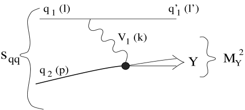
Figure 6: The Feynman diagram in the effective vector-boson approximation for the scattering of a quark $q_{1}$ with a quark $q_{2}$ at a scattering energy $\sqrt{s_{qq}}$. A final state $Y$ with the squared invariant mass $M_{Y}^{2}$ is produced. The particle $V_{1}$ is an exchanged vector-boson. The four-momenta of the particles are denoted by $l,l^{\prime},k$ and $p$.

We give an approximation to the exact luminosities which is obtained from the full expression (9). It has been shown in [19] how the expression (7) reduces to a convolution of vector-boson distributions if certain kinematical approximations are made. The approximate expression for (7) is given by

$${\cal L}_{V_{1},V_{2},\lambda_{1}\lambda_{2}}^{q_{1}q_{2}}(\hat{x})=\eta_{0}\int\limits_{\hat{x}}^{1}\frac{d\hat{z}}{\hat{z}}{f}_{V_{1},\lambda_{1}}^{q_{1}}\left(\hat{z},\frac{M_{1}^{2}}{s_{qq}}\right){f}_{V_{2},\lambda_{2}}^{q_{2}}\left(\frac{\hat{x}}{\hat{z}},\frac{M_{2}^{2}}{\hat{z}\,s_{qq}}\right),$$ (21)

where the functions ${f}_{V_{T}}^{q}$, ${f}_{V_{\overline{T}}}^{q}$ and ${f}_{V_{L}}^{q}$ (we use $V=V_{i}$, $q=q_{i}$ etc. if no distinction between two different particles is necessary) are the distribution functions of vector-bosons in fermions of [23]. The label $\lambda=T,\overline{T},L$ denotes the helicity of the vector-boson. Distribution functions of vector-bosons in fermions describe the process shown in Figure 6. The cross-section for the process in Figure 6, averaged over the helicity of the quark $q_{1}$ and summed over the helicity of the quark $q^{\prime}_{1}$, is given in terms of $f_{V_{\lambda}}^{q}$ by the expression

$$\sigma(q_{1}q_{2}\to q_{1}^{\prime}Y,s_{qq})=\sum_{V_{1},\lambda_{1}}\int\limits_{0}^{1}d\hat{z}f_{V_{1,\lambda_{1}}}^{q_{1}}\left(\hat{z},\frac{M_{1}^{2}}{s_{qq}}\right)\sigma(V_{1,\lambda_{1}}q_{2}\to Y,M_{Y}^{2}=\hat{z}s_{qq}).$$ (22)

The distribution function $f_{V_{\lambda}}^{q}\left(\hat{z},M^{2}/s_{qq}\right)$ is the probability density for the emission of a vector-boson $V$ with the helicity $\lambda$ and mass $M$ from a fermion $q$. Separating the fermionic couplings, the $f_{V_{\lambda}}^{q}$ can be written as

$$f_{V_{\lambda}}^{q}\left(\hat{z},\frac{M^{2}}{s_{qq}}\right)=\frac{\alpha}{2\pi}\hat{z}c_{q(V)}^{\lambda}h_{\lambda}\left(\hat{z},\frac{M^{2}}{s_{qq}}\right).$$ (23)

The quantities $h_{\lambda}$ in (23) are “amputated” vector-boson distribution functions. The specific functions of [23] have to be taken. Amputated distribution functions do not depend on the fermionic couplings but only on two dimensionless variables. Equivalent to (21), for the corresponding amputated differential luminosities one obtains the forms

$${\cal L}_{\lambda_{1}\lambda_{2}}\left(\hat{x},\hat{z},\frac{M_{1}^{2}}{s_{qq}},\frac{M_{2}^{2}}{s_{qq}}\right)=\eta_{0}\,{h}_{\lambda_{1}}\left(\hat{z},\frac{M_{1}^{2}}{s_{qq}}\right){h}_{\lambda_{2}}\left(\frac{\hat{x}}{\hat{z}},\frac{M_{2}^{2}}{\hat{z}\,s_{qq}}\right).$$ (24)

The amputated distribution functions ${h}_{T}$, ${h}_{\overline{T}}$ and ${h}_{L}$ have been given in closed form in [23].

We introduce a useful approximation to (24). The form of the luminosities (21), (24) is not invariant under the simultaneous exchange of the vector-bosons $V_{1}$ and $V_{2}$ (i.e., their masses, fermionic couplings and helicities $\lambda_{1}$ and $\lambda_{2}$) and the fermions $q_{1}$ and $q_{2}$. The luminosities (7), however, obey this symmetry. The symmetry is broken by the approximations which led to (24). The symmetry of (24) is not present because different energies are available for the emission processes of $V_{1}$ and $V_{2}$. The available energy for the emission of $V_{2}$ is reduced if $V_{1}$ is emitted in addition. We extract from this fact that an approximation to (7) should feature an effective reduction of the available fermion-fermion scattering energy. The reduction is due to the simultaneous emission of two vector-bosons. We introduce the symmetrized form

$${\cal L}_{\lambda_{1}\lambda_{2}}\left(\hat{x},\hat{z},\frac{M_{1}^{2}}{s_{qq}},\frac{M_{2}^{2}}{s_{qq}}\right)=\eta_{0}\,{h}_{\lambda_{1}}\left(\hat{z},\frac{M_{1}^{2}}{\sqrt{\hat{z}}s_{qq}}\right){h}_{\lambda_{2}}\left(\frac{\hat{x}}{\hat{z}},\frac{M_{2}^{2}\,\sqrt{\hat{z}}}{\sqrt{\hat{x}}s_{qq}}\right).$$ (25)

In (25), the available energies for the emission of $V_{1}$ and $V_{2}$ are $\sqrt{\hat{z}}s_{qq}$ and $\sqrt{\hat{x}/\hat{z}}s_{qq}$, respectively. Eq. (25) is an approximation to Eq. (24). We refer to the luminosities (16) using (25) as Approximation 1.

Figure 7: The ratio of the luminosities using the approximations (25) or (34) and the exact luminosities, Eq. (9), for finding a $W^{+}Z$ pair in a proton pair of $\sqrt{s_{hh}}=14$ TeV for the diagonal helicity combinations as a function of the variable $x$. In Figure a, the direct approximation, Eq. (25), was used. In Figures b, c and d, the vector-boson distributions of [23], Eq. (67) (DGC) and the LLA, respectively, were used to evaluate ${\cal L}_{pol}$ according to Eq. (34). All luminosities have been calculated according to Eq. (16).

Figure 7 a shows the ratios of the luminosities (16), evaluated with (25), and the exact luminosities, (16) with (9), for the diagonal helicity combinations as a function of $x$. The region $10^{-3}\;\raisebox{-3.00003pt}{$\stackrel{{\scriptstyle\displaystyle<}}{{\sim}}$}\;x\;\raisebox{-3.00003pt}{$\stackrel{{\scriptstyle\displaystyle<}}{{\sim}}$}\;2\cdot 10^{-2}$ is particularly interesting for vector-boson pair production. It corresponds to invariant masses of $400$ GeV $\;\raisebox{-3.00003pt}{$\stackrel{{\scriptstyle\displaystyle<}}{{\sim}}$}\;M_{V_{3}V_{4}}\;\raisebox{-3.00003pt}{$\stackrel{{\scriptstyle\displaystyle<}}{{\sim}}$}\;2$ TeV. In this region, the dominant $TT$ luminosity deviates by less than $30\%$ from the exact result. A comparison with results of other authors will be given in Section 2.3.

Further approximations may be applied. So far we have employed approximate expressions for the ${\cal L}_{V_{1},V_{2},pol}^{q_{1}q_{2}}(\hat{x})$ but we used the correct expression for the quark-quark subenergy, $s_{qq}\equiv\tau s_{hh}$. If approximate expressions for $s_{qq}$ are used, the luminosity ${\cal L}_{(V_{1}V_{2})_{pol}}^{h_{1}h_{2}}(x)$ can be approximated as a convolution of vector-boson distribution functions $f_{V_{\lambda}}^{h}$ in hadrons. Luminosities have been previously obtained in this way [5, 21]. The possibility to use vector-boson distributions in hadrons has already been mentioned in [3]. An equivalent expression for (16) is

$${\cal L}_{(V_{1}V_{2})_{pol}}^{h_{1}h_{2}}(x) = C_{(12)}\left(\frac{\alpha}{2\pi}\right)^{2}x\int\limits_{x}^{1}\frac{dz}{z}\int\limits_{z}^{1}\frac{d\xi_{1}}{\xi_{1}}\int\limits_{x/z}^{1}\frac{d\xi_{2}}{\xi_{2}}\frac{1}{\xi_{1}\xi_{2}}$$ (27)

$$\times\left[\left(\sum_{q_{1}(V_{1})}c_{q_{1}(V_{1})}^{pol}f_{q_{1}}^{h_{1}}(\xi_{1},\mu_{1}^{2})\right)\cdot\left(\sum_{q_{2}(V_{2})}c_{q_{2}(V_{2})}^{pol}f_{q_{2}}^{h_{2}}(\xi_{2},\mu_{2}^{2})\right)\;\;+\;\;h_{1}\leftrightarrow h_{2}\,\right]$$

$$\cdot{\cal L}_{pol}\left(\hat{x}=\frac{x}{\xi_{1}\xi_{2}},\hat{z}=\frac{z}{\xi_{1}},\frac{M_{1}^{2}}{s_{qq}},\frac{M_{2}^{2}}{s_{qq}}\right),$$

where we introduced the variable $z=\xi_{1}\hat{z_{1}}$. The variable $z$ describes the invariant mass squared $M_{Y}^{2}$ which is left for the reaction of the vector-boson $V_{1}$ with the quark $q_{2}$. If $V_{1}$ is light-like, $z$ is equal to the ratio of the energy of $V_{1}$ and the energy of the hadron from which it was emitted. In analogy to $\hat{z}_{1}$ and $\hat{z}_{2}$ we introduce the variables $z_{1}=z$ and $z_{2}=x/z$. It follows that $z_{i}=\xi_{i}\hat{z}_{i}$. Inserting the convolutions (25) into (27) leads to the expression

$${\cal L}_{(V_{1}V_{2})_{\lambda_{1}\lambda_{2}}}^{h_{1}h_{2}}(x) = C_{(12)}\,\eta_{0}\int\limits_{x}^{1}\frac{dz}{z}\int\limits_{z}^{1}d\xi_{1}\int\limits_{x/z}^{1}d\xi_{2}$$ (28)

$$\cdot\left[\frac{df_{V_{1,\lambda_{1}}}^{h_{1}}}{d\xi_{1}}(z)\frac{df_{V_{2,\lambda_{2}}}^{h_{2}}}{d\xi_{2}}\left(\frac{x}{z}\right)\;\;+\;\;h_{1}\leftrightarrow h_{2}\,\right].$$

In (28), the quantities $df_{V_{\lambda}}^{h}/d\xi$ are differential distribution-functions of a vector-boson $V_{\lambda}$ in a hadron $h$. They are given by

$$\xi\frac{df_{V_{\lambda}}^{h}}{d\xi}(z) = \frac{\alpha}{2\pi}\frac{z}{\xi}\sum_{q(V)}c_{q(V)}^{\lambda}f_{q}^{h}(\xi,\mu^{2})h_{\lambda}\left(\frac{z}{\xi},\frac{M^{2}\sqrt{\xi}}{\sqrt{z}\,s_{qq}}\right),$$ (29)

with $s_{qq}=\xi_{1}\xi_{2}s_{hh}$.

The integrations over $\xi_{1}$ and $\xi_{2}$ in (28) cannot be carried out independently because $s_{qq}$ in the differential distributions (29) depends on both $\xi_{1}$ and $\xi_{2}$. We may, however, approximate $s_{qq}$ by $s_{qq}=\xi_{i}^{2}s_{hh}$. It means that we assume the same energy, $E=\xi_{i}E_{h}$, for the quark which emits the vector-boson $V_{i}$ and the other quark which emits $V_{j}$. $E_{h}$ is the hadron energy evaluated in the hadron-hadron cms, $E_{h}=\sqrt{s_{hh}}/2$. Equivalently, it means that the parton-parton cms is approximated as the hadron-hadron cms. With this approximation the vector-boson distributions in a hadron are given by

$$f_{V_{\lambda}}^{h}(z)=\int\limits_{z}^{1}\frac{d\xi}{\xi}\sum_{q(V)}f_{q}^{h}(\xi,\mu^{2})f_{V_{\lambda}}^{q}\left(\frac{z}{\xi},\frac{M^{2}\sqrt{\xi}}{\sqrt{z}s_{qq}}\right),$$ (30)

with $s_{qq}=\xi^{2}s_{hh}$ and $f_{V_{\lambda}}^{q}(\hat{z}=z/\xi)$ from (23). We require $z/\xi>M^{2}/s_{qq}$, i.e., $\xi_{min}=\max[z,M^{2}/(zs_{hh})]$ as the lower limit of integration in (30). Again, as in (21), the functions (30) do not contain a flux factor since the boson-boson flux factor $\eta_{0}$ already appears explicitly in front of the integral in (28).

The luminosities ${\cal L}_{(V_{1}V_{2})}^{h_{1}h_{2}}(x)$ are given by using the functions (30) in Eq. (28),

$${\cal L}_{(V_{1}V_{2})_{\lambda_{1}\lambda_{2}}}^{h_{1}h_{2}}(x)=C_{(12)}\,\eta_{0}\int\limits_{\frac{1}{2}\ln(x)}^{-\frac{1}{2}\ln(x)}dy\left[f_{V_{1,\lambda_{1}}}^{h_{1}}\left(\sqrt{x}e^{y}\right)f_{V_{2,\lambda_{2}}}^{h_{2}}\left(\sqrt{x}e^{-y}\right)\;+\;h_{1}\leftrightarrow h_{2}\,\right],$$ (31)

where we introduced the variable

$$y\equiv\frac{1}{2}\ln\left(z^{2}/x\right)=\frac{1}{2}\ln\left(\frac{z_{1}}{z_{2}}\right)=y_{q}+\hat{y}.$$ (32)

If the vector-bosons $V_{1},V_{2}$ are light-like, $y$ is the rapidity of the $V_{1}V_{2}$ center-of-mass motion taken along the direction of motion of the hadron which emitted $V_{1}$. The formula (31) has been derived with only the mentioned approximations (using the factorized forms (25) and approximating $s_{qq}$ by $s_{qq}\simeq\xi^{2}s_{hh}$) from the exact luminosities for a vector-boson pair in a proton-pair, (16) with (9). We refer to (31) as Approximation 2. It is a direct approximation to the exact luminosities.

Figure 8: The ratio of the luminosities approximated as convolutions of vector-boson distribution functions $f_{V_{\lambda}}^{p}$ and the exact luminosities for finding a $W^{+}Z$ pair in a proton pair of $\sqrt{s_{hh}}=14$ TeV for the diagonal helicity combinations as a function of the variable $x$. In Figure a, Eq. (31) was used to evaluate $f_{V_{\lambda}}^{q}$ in (35). In Figures b, c and d, Eq. (38) was used and the vector-boson distributions of [5], Eq. (67) (DGC) and the LLA, respectively, were used.

Figure 8 a shows the ratios of the luminosities in Approximation 2, Eq. (31), and the exact luminosities for finding a $W^{+}Z$ pair in a proton pair of $\sqrt{s_{hh}}=14$ TeV for the diagonal helicity combinations as a function of $x$. The Approximation 2 is in excellent agreement with the improved EVBA. The results of other authors will be discussed in the following Section.

2.3 Comparison with the Literature

The exact luminosities (16) with (9) may be compared with results presented in the literature [3, 5, 21]. In contrast to the approximations (25) and (31), these results do not use the exact expression as a starting point. Instead, they use the ad hoc assumption that the luminosities ${\cal L}_{V_{1},V_{2},pol}^{q_{1}q_{2}}(\hat{x})$ can be obtained by convolutions of vector-boson distribution functions. The convolution is similar to (21) and is given by

$${\cal L}_{V_{1},V_{2},\lambda_{1}\lambda_{2}}^{q_{1}q_{2}}(\hat{x})=\int\limits_{\hat{x}}^{1}\frac{d\hat{z}}{\hat{z}}f_{V_{1,\lambda_{1}}}^{q_{1}}\left(\hat{z},\frac{M_{1}^{2}}{s_{qq}}\right)f_{V_{2,\lambda_{2}}}^{q_{2}}\left(\frac{\hat{x}}{\hat{z}},\frac{M_{2}^{2}}{s_{qq}}\right).$$ (33)

Instead of the particular functions $f_{V_{\lambda}}^{q}$ of [23], various different functions have been used. Equivalent to the approximation (33), the amputated differential luminosities are written as a product of amputated distribution functions,

$${\cal L}_{\lambda_{1}\lambda_{2}}\left(\hat{x},\hat{z},\frac{M_{1}^{2}}{s_{qq}},\frac{M_{2}^{2}}{s_{qq}}\right)=h_{\lambda_{1}}\left(\hat{z},\frac{M_{1}^{2}}{s_{qq}}\right)h_{\lambda_{2}}\left(\frac{\hat{x}}{\hat{z}},\frac{M_{2}^{2}}{s_{qq}}\right).$$ (34)

Vector-boson distribution functions have been derived by several authors [3, 4, 5, 21, 23, 25, 26, 28]. In most cases more assumptions than only the ones inherent in the EVBA, i.e. that the reaction proceeds via the exchange of vector-bosons and that the vector-boson scattering cross-sections for off-shell vector-bosons must be known (or an assumption has to be made), were made in the derivation. The differences of various derivations are discussed in Appendix A. In the Appendix we also specify the vector-boson distribution functions $f_{V_{\lambda}}^{q}$ which we use for our numerical examples.

Figures 7 b,c and d show the ratios of the approximated luminosities, Eq. (16) evaluated with (34), and the exact luminosities, (16) with (9), using for $h_{\lambda}$ the distributons [23], the distributions (67) and the LLA, respectively, for the diagonal helicity combinations as a function of $x$. The LLA overestimates the improved EVBA by an order of magnitude at small $x$ if both polarizations are transverse. Using (67) or [23], instead, greatly diminishes the deviation of the approximation from the improved EVBA. We note that the better agreement of the distributions (67) than the one of the distributions [23] with the improved EVBA is accidental since the distributions (67) involve additional approximations as compared to the distributions [23] (see Appendix A). One sees that the use of Eq. (25) (Figure 7 a) further improves the agreement between approximated and exact luminsoities, at least compared to the convolutions of [23]. In particular, the agreement is substantially improved for the dominating $TT$ luminosity.

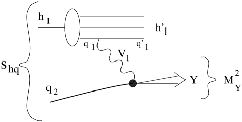
Figure 9: The diagram for the scattering of a hadron $h_{1}$ and a quark $q_{2}$ proceeding via the exchange of a single vector-boson $V_{1}$ originating from the hadron. A final state $Y$ of invariant mass $M_{Y}$ is produced.

Similarly to Approximation 2, vector-boson distribution functions in hadrons have been used. They were derived in order to describe the process shown in Figure 9. The distribution functions were obtained as convolutions of the quark distributions in hadrons and the vector-boson distributions in quarks,

$$f_{V_{\lambda}}^{h}(z)=\int\limits_{z}^{1}\frac{d\xi}{\xi}\sum_{q(V)}f_{q}^{h}(\xi,\mu_{i}^{2})f_{V_{\lambda}}^{q}\left(\frac{z}{\xi},\frac{M^{2}}{s_{qq}}\right).$$ (35)

The functions $f_{V_{\lambda}}^{h}$ describe the emission probability of a vector-boson $V$ with helicity $\lambda$ and mass $M$ from a hadron $h$. The sum in (35) extends over all quarks and antiquarks which can couple to $V$. Eq. (35) is similar to (30). However, in (30) the specific distributions [23] have to be used. In addition, in (30) we included the square roots introduced in (25). The definition of $z$ in terms of $s_{hq}$ (defined in Figure 9) and $M_{Y}^{2}$ is given by

$$z\equiv M_{Y}^{2}/s_{hq}.$$ (36)

The cross-section for the process shown in Figure 9 is given by

$$\sigma(h_{1}q_{2}\to h_{1}^{\prime}Y,s_{hq})=\sum_{V_{1},\lambda_{1}}\int\limits_{0}^{1}dzf_{V_{1,\lambda_{1}}}^{h_{1}}\left(z,\frac{M_{1}^{2}}{s_{qq}}\right)\sigma(V_{1,\lambda_{1}}q_{2}\to Y,M_{Y}^{2}).$$ (37)

In writing down (37) no other assumptions than those inherent in the EVBA have been made.

The quark-quark energy $s_{qq}$ is in principle unknown if only the energy $E_{h}$ of the hadron or the hadron-hadron scattering energy $s_{hh}$ is known. Thus, an approximation for $s_{qq}$ has to be made. We will again use $s_{qq}\simeq\xi^{2}s_{hh}$, as above.

In [33], a variable $Q^{2}$, which was defined by $Q^{2}\equiv M_{Y}^{2}$ was used. The approximation $s_{qq}\simeq\xi^{2}s_{hh}$ applied to $Q^{2}$ is $Q^{2}=\hat{z}s_{qq}=z/\xi s_{qq}\simeq z\xi s_{hh}$.

The luminosities ${\cal L}_{(V_{1}V_{2})_{\lambda_{1}\lambda_{2}}}^{h_{1}h_{2}}(x)$ were approximately expressed as convolutions of the vector-boson distribution functions (35),

$${\cal L}_{(V_{1}V_{2})_{\lambda_{1}\lambda_{2}}}^{h_{1}h_{2}}(x)=C_{(12)}\int\limits_{\frac{1}{2}\ln(x)}^{-\frac{1}{2}\ln(x)}dy\left[f_{V_{1,\lambda_{1}}}^{h_{1}}\left(\sqrt{x}e^{y}\right)f_{V_{2,\lambda_{2}}}^{h_{2}}\left(\sqrt{x}e^{-y}\right)\;+\;h_{1}\leftrightarrow h_{2}\,\right].$$ (38)

The approximation (38) has often been used in the past and numerical results for the luminosities can be found in [21, 33].

We note that in [33] an excellent approximation was made. As discussed above, instead of the variable $s_{qq}$ two variables $Q_{1}^{2}$ and $Q_{2}^{2}$, which appear in $f_{V_{1,\lambda_{1}}}^{h_{1}}$ and $f_{V_{2,\lambda_{2}}}^{h_{2}}$, respectively, were used. The $Q_{i}^{2}$ are the squared invariant masses of a vector-boson and a quark which are defined in terms of $s_{qq}$, or, alternatively, in terms of $s_{hh}$ by

$$Q_{i}^{2}\equiv\hat{z}_{i}s_{qq}=\frac{z_{i}}{\xi_{i}}s_{qq}=x\frac{\xi_{j}}{z_{j}}s_{hh},\quad i\neq j,\quad i=1,2,$$ (39)

where we have only used the exact relations $s_{qq}=\xi_{1}\xi_{2}s_{hh}$ and $z_{1}z_{2}=x$. Clearly, again, factorization does not occur using the exact expressions (39). Instead of using the approximation $s_{qq}\simeq\xi_{i}^{2}s_{hh}$, another approximation for the $Q_{i}^{2}$ has been made in [33] when luminosities were calculated, namely the simple approximate choice $Q_{i}^{2}\simeq xs_{hh}={\cal W}^{2}$. Thus, the quark vector-boson invariant masses $Q_{i}^{2}$ have been approximated by the vector-boson vector-boson invariant mass. This choice always underestimates the exact values of $Q_{i}^{2}$. However, we know that reducing the invariant masses involving quarks will in general improve the agreement with the improved EVBA. We will therefore use this choice of $Q_{i}^{2}$ in our numerical example below. It leads to an excellent agreement with the improved EVBA. For the other distributions $f_{V_{\lambda}}^{h}$, we use $s_{qq}\simeq\xi_{i}^{2}s_{hh}$ as before.

Figures 8 b,c and d show the ratios of the luminosities calculated according to Eq. (38) and the exact luminosities for finding a $W^{+}Z$ pair in a proton pair of $\sqrt{s_{hh}}=14$ TeV for the diagonal helicity combinations as a function of $x$. To evaluate (38), the distributions of [5] (using $Q_{i}^{2}={\cal W}^{2}$), the distributions (67) and the LLA were used. The LLA overestimates the exact luminosities by far. The distributions (67) yield slightly low values at low $x$. The distributions [5] are an excellent approximation to the improved EVBA. For the dominant $TT$ luminosity, the direct approximation (Figure 8 a) is better than the distributions [5].

Figure 10: The distribution functions of a $W^{+}$ boson in a proton of $E_{h}=\sqrt{s_{hh}}=7$ TeV, Eq. (30) (This work) or (35) (all others), for the helicity combinations $T$, $\overline{T}$ and $L$ as a function of $z$. The LLA, Eq. (67) (DGC) and the distributions [5] and [23] were used to evaluate $f_{V_{\lambda}}^{q}$ in (35).

We finally present numerical results for the vector-boson distribution functions in hadrons. In the numerical example of the functions (30) we approximate the boson-boson flux factor in (28) by a product of boson-quark flux factors,

$$\eta_{0}\simeq\left(1-\frac{M_{1}^{2}}{\hat{z}_{1}s_{qq}}\right)\left(1-\frac{M_{2}^{2}}{\hat{z}_{2}s_{qq}}\right).$$ (40)

One of the boson-quark flux factors, $\left(1-\frac{M^{2}}{\hat{z}s_{qq}}\right)$, is then included in the $f_{V_{\lambda}}^{q}(\hat{z}=z/\xi)$ in (30). Figure 10 shows the distributions functions for a $W^{+}$ in a proton of $E_{h}=\sqrt{s_{hh}}/2=7$ TeV for the various helicity combinations of the $W^{+}$ as a function of $z$. The distribution functions have been calculated according to Eq. (30) or Eq. (35). To evaluate Eq. (35), the LLA, the distributions (67) and those of [5] and [23] have been used for $f_{V_{\lambda}}^{q}$. We note that we used the complete expressions [5] instead of the next-to leading forms [33].

For the $T$- and $\overline{T}$-polarization, the LLA overestimates any of the other distributions by far. The distributions [23] are larger than those of Eq. (30). The distributions (67) yield rather low values. The differences between the distributions increase at small $z$. For the $L$-polarization, the differences between the models only manifest themselves at low values of $z$.

We note that a typical value for $z$ is $z=\sqrt{x}\simeq 7\cdot 10^{-2}$ if a final state $\Xi$ of mass 1 TeV is produced in $pp$-collisions at $\sqrt{s_{hh}}=14$ TeV. All values of $z$ in the range $x<z<1$, however, contribute to the integral in (31) or (38). For ${\cal W}=450$ GeV, which is still a large energy compared to the vector-boson masses, $z$ becomes as small as $z=x\simeq 10^{-3}$ and the whole range of $z$ which is shown in Figure 10 contributes to the luminosity.

3 Comparison with a Complete Perturbative Calculation

We are now going to present a numerical comparison of the EVBA with a complete perturbative calculation. The complete perturbative calculation includes the contribution from bremsstrahlung diagrams as shown in Figure 3. As an example for a vector-boson pair production process, we choose the process $pp\to ZZX$, for which complete results are available in the literature.

The complete perturbative calculation uses in Eq. (4) the complete (lowest order) cross-section of the process on the quark-level, $q_{1}q_{2}\to q_{1}^{\prime}q_{2}^{\prime}ZZ$. Numerical results of the complete calculation for $\sqrt{s}=40$ TeV can be found in [29] and [25, 30]. Only the production via $W^{+}W^{-}$-pairs, $pp\to W^{+}W^{-}\to ZZ$, was considered.

In the EVBA one has to calculate the cross-sections for $W^{+}W^{-}\to ZZ$. In the Born approximation there are four diagrams which contribute to these processes. Two diagrams describe the exchange of massive vector-bosons, one diagram a four-particle point interaction and one diagram Higgs boson exchange. An analytical expression for the helicity amplitudes has been given in [31].

As in [25], we apply a rapidity cut on the produced vector-bosons $V_{3}V_{4}=ZZ$ in the hadron-hadron cms frame. We treat this cut approximately assuming that the vector-bosons $V_{1},V_{2}$ move collinearly to the hadron beam direction. The rapidities of the vector-bosons $V_{3}$ and $V_{4}$ in the $V_{1}V_{2}$ cms frame, taken along the direction of motion of the hadron from which $V_{1}$ is emitted, are

$$y_{3}^{\ast}=\tanh^{-1}\left(\frac{q\cos\theta}{\sqrt{q^{2}+M_{3}^{2}}}\right),\quad\quad y_{4}^{\ast}=\tanh^{-1}\left(\frac{-q\cos\theta}{\sqrt{q^{2}+M_{4}^{2}}}\right).$$ (41)

In (41), $\theta$ is the angle between the directions of motion of $V_{1}$ and $V_{3}$ evaluated in the $(V_{1}V_{2})$ center-of-mass system. The variable $q$ is the magnitude of the space-like momentum of the vector-boson $V_{3}$ in this system,

$$q=\frac{\sqrt{{\cal W}^{2}}}{2}\sqrt{1-\frac{2}{{\cal W}^{2}}(M_{3}^{2}+M_{4}^{2})+\frac{1}{{\cal W}^{4}}(M_{3}^{2}-M_{4}^{2})^{2}}.$$ (42)

The rapidities $y_{3},y_{4}$ of $V_{3},V_{4}$ in the hadron-hadron cms frame are approximately obtained by addition, $y_{3}\simeq y+y_{3}^{\ast}$ and $y_{4}\simeq y+y_{4}^{\ast}$, where the equality holds strictly if both $V_{1}$ and $V_{2}$ are light-like. We apply a rapidity cut $Y$ to both produced vector-bosons,

$$|y_{3}|<Y\;\;\mbox{and}\;\;|y_{4}|<Y.$$ (43)

Following from (13) and (16) with (17), we obtain the expression for the cross-section for $h_{1}h_{2}\to V_{1}V_{2}\to V_{3}V_{4}$ with a rapidity cut,

$$\frac{d\sigma}{dx}(h_{1}h_{2}\to V_{1}V_{2}\to V_{3}V_{4},s_{hh})\theta(Y-|y_{3}|)\theta(Y-|y_{4}|)$$ (44)

$$= \left(\frac{\alpha}{2\pi}\right)^{2}x\int\limits_{-y_{\mathrm{max}}}^{y_{\mathrm{max}}}dy\int\limits_{0}^{\ln\left(\frac{1}{x}\right)}\frac{d\ln\left(\frac{1}{\tau}\right)}{\tau}\int\limits_{\max[-\frac{1}{2}\ln\left(\frac{1}{\tau}\right),-\frac{1}{2}\ln\left(\frac{\tau}{x}\right)+y]}^{\min[\frac{1}{2}\ln\left(\frac{1}{\tau}\right),\frac{1}{2}\ln\left(\frac{\tau}{x}\right)+y]}dy_{q}\sum_{(V_{1}V_{2})}C_{(12)}\,\eta_{0}\sum_{pol}$$ (48)

$$\cdot\Bigg{[}\left(\sum_{q_{1}(V_{1})}f_{q_{1}}^{h_{1}}(\sqrt{\tau}e^{y_{q}},\mu_{1}^{2})c_{q_{1}(V_{1})}^{pol}\right)\cdot\left(\sum_{q_{2}(V_{2})}f_{q_{2}}^{h_{2}}(\sqrt{\tau}e^{-y_{q}},\mu_{2}^{2})c_{q_{2}(V_{2})}^{pol}\right)$$

$$\quad\quad\cdot{\cal L}_{pol}\left(\hat{x},\sqrt{\frac{x}{\tau}}e^{y-y_{q}},\frac{M_{1}^{2}}{s_{qq}},\frac{M_{2}^{2}}{s_{qq}}\right)\quad+\quad h_{1}\leftrightarrow h_{2}\;\;\Bigg{]}$$

$$\cdot\int\limits_{z_{\mathrm{min}}(y)}^{z_{\mathrm{max}}(y)}d\cos\theta\frac{d\sigma}{d\cos\theta}((V_{1}V_{2})_{pol}\to V_{3}V_{4},{\cal W}^{2}),$$

where the integration limits are determined by the rapidity-cut,

$$y_{\mathrm{max}} = \min\left[Y,\frac{1}{2}\left(\frac{1}{x}\right)\right],$$ (49)

$$z_{\mathrm{min}}(y) = \max\left[\frac{-\tanh(Y+y)}{\beta(M_{3}^{2},M_{4}^{2})},\frac{-\tanh(Y-y)}{\beta(M_{4}^{2},M_{3}^{2})},-\cos\theta_{\mathrm{min}}\right],$$ (50)

$$z_{\mathrm{max}}(y) = \min\left[\frac{\tanh(Y-y)}{\beta(M_{3}^{2},M_{4}^{2})},\frac{\tanh(Y+y)}{\beta(M_{4}^{2},M_{3}^{2})},\cos\theta_{\mathrm{min}}\right],$$ (51)

with

$$\beta(M^{2},{M^{\prime}}^{2}) \equiv \frac{\sqrt{1-\frac{2}{{\cal W}^{2}}(M^{2}+{M^{\prime}}^{2})+\frac{1}{{\cal W}^{4}}(M^{2}-{M^{\prime}}^{2})^{2}}}{1+\frac{M^{2}-{M^{\prime}}^{2}}{{\cal W}^{2}}}$$ (52)

$$= \frac{q}{\sqrt{q^{2}+M^{2}}},$$ (53)

and $\cos\theta_{\mathrm{min}}=1$. In the vicinity of the threshold for the production of the pair $V_{3}V_{4}$, the rapidity-cut has no effect anymore, i.e. $z_{\mathrm{max}}(y)$ and $z_{\mathrm{min}}(y)$ are determined by $\cos\theta_{\mathrm{min}}=1$.

If the masses of the vector-bosons $V_{3}$ and $V_{4}$ are equal or only slightly different, $M_{3}^{2}\simeq M_{4}^{2}$, or if the momenta of the bosons are large against their masses, $q^{2}\gg\max(M_{3}^{2},M_{4}^{2})$, the expressions (51) for $z_{\mathrm{min}}$ and $z_{\mathrm{max}}$ simplify to give $z_{\mathrm{max}}=-z_{\mathrm{min}}=z_{0}$, where

$$z_{0}=\min\left[\frac{\tanh(Y-|y|)}{\beta(M_{3}^{2},M_{4}^{2})},\cos\theta_{\mathrm{min}}\right].$$ (54)

If one applies a rapidity cut to the expression for convolutions of vector-boson distributions, (31) with (30), one obtains the expression

$$\frac{d\sigma}{dx}(h_{1}h_{2}\to V_{1}V_{2}\to V_{3}V_{4},s_{hh})|_{\mathrm{Cut}}$$ (55)

$$= \sum_{(V_{1}V_{2})}C_{(12)}\,\eta_{0}\sum_{pol=\lambda_{1}\lambda_{2}}\int\limits_{-y_{max}}^{y_{max}}dy\left[f_{V_{1,\lambda_{1}}}^{p_{1}}(\sqrt{x}e^{y},\mu_{1}^{2})f_{V_{2,\lambda_{2}}}^{p_{2}}(\sqrt{x}e^{-y},\mu_{2}^{2})\;\;+\;\;h_{1}\leftrightarrow h_{2}\;\right]$$ (57)

$$\quad\quad\quad\quad\quad\quad\quad\quad\quad\cdot\int\limits_{z_{\mathrm{min}}(y)}^{z_{\mathrm{max}}(y)}d\cos\theta\frac{d\sigma}{d\cos\theta}((V_{1}V_{2})_{\lambda_{1}\lambda_{2}}\to V_{3}V_{4},{\cal W}^{2}),$$

with $y_{max},z_{\mathrm{min}}(y)$ and $z_{\mathrm{max}}(y)$ from (51).

We calculate the differential cross-section $d\sigma/dM_{ZZ}$ from Eq. (48) with the luminosities of the improved EVBA. As in [25], the quark-distributions of EHLQ, [32], set 2, are used and the electroweak parameters are $\alpha=1/128,s_{W}^{2}=0.22,M_{W}=80$ GeV, $M_{H}=0.5$ TeV and $\Gamma_{H}=51.5$ GeV. For the scales $\mu_{i}^{2}$ in the quark-distributions, $\mu_{i}^{2}=s_{qq}/4$ is chosen. We also carry out a calculation with the convolutions of vector-boson distributions from Eq. (57).

Figure 11 shows the cross-section for $pp\to W^{+}W^{-}\to ZZ$ at a scattering energy of $\sqrt{s_{hh}}=40$ TeV as a function of the invariant mass $M_{ZZ}$ of the $ZZ$ pair for rapidity cuts of $Y=2.5$ and $Y=1.5$ as a result of the improved EVBA calculation and the calculation with convolutions of vector-boson distributions together with the complete result from [25]. For $Y=2.5$, the cross-section of the improved EVBA deviates by a factor of two from the complete result at $M_{ZZ}\;\raisebox{-3.00003pt}{$\stackrel{{\scriptstyle\displaystyle>}}{{\sim}}$}\;0.7$ TeV. The result obtained with the convolutions deviates by $13\%$ ($M_{ZZ}=1.2$ TeV) and $18\%$ ($M_{ZZ}=0.6$ TeV) from the improved EVBA result, independently of the magnitude of the cut. For $Y=1.5$, a good agreement between the improved EVBA and the complete calculation is found. The EVBA deviates by less than $10\%$ from the exact result for $M_{ZZ}>0.4$ TeV.

An explanation for the different results for $Y=2.5$ and $Y=1.5$ is that the bremsstrahlung-type diagrams in Fig. 3 begin to play a role if the angle between the produced vector-boson and the hadron beam-direction is small. This is the case for $Y=2.5$. In contrast, the bremsstrahlung-diagrams might be neglected if only large angles are involved. This is the case for $Y=1.5$. For a cut of $Y=2.5$ the smallest allowed angle is $\theta_{\mathrm{min}}=9.4^{\circ}$, while the smallest angle for $Y=1.5$ is $\theta_{\mathrm{min}}=25.2^{\circ}$.

In summary, we have seen that the improved EVBA deviates by only ${\cal O}(10\%)$ from the result of a complete perturbative calculation for a cut of $Y=1.5$. This result was found for $pp\to ZZ+X$ at $\sqrt{s_{hh}}=40$ TeV and invariant masses of $\sqrt{{\cal W}^{2}}>0.4$ TeV. There is, however, no reason that a similar conclusion could not also be drawn for the production of other vector-boson pairs, $pp\to V_{3}V_{4}+X$. We expect this because the EVBA only pertains to the process-independent vector-boson luminosities. The use of convolutions instead of the improved EVBA leads to an additional error of $<20\%$ for $\sqrt{{\cal W}^{2}}\;\raisebox{-3.00003pt}{$\stackrel{{\scriptstyle\displaystyle>}}{{\sim}}$}\;0.5$ TeV ($10\%$ at $\sqrt{{\cal W}^{2}}=2$ TeV).

Figure 11: The cross-section for $pp\to ZZX$ via $W^{+}W^{-}$-scattering as a function of the invariant mass $M_{ZZ}$ at $\sqrt{s_{hh}}=40$ TeV. A rapidity cut of $Y=2.5$ and $Y=1.5$ was applied. Shown is the result of the complete perturbative calculation [25], the improved EVBA (48) and the result of the convolutions of vector-boson distributions (57).

We finally present another result which is of interest in connection with the EVBA. It concerns the magnitude of the off-diagonal terms in the helicities of $V_{1}$ and $V_{2}$, denoted by $TTTT$, $TLTL$ and $\overline{T}L\overline{T}L$ in [19]. Figure 12 shows the contributions of the $LL$-, the other diagonal, the non-diagonal and the sum of all helicity combinations for the cross-section for $pp\to(W^{+}W^{-}+ZZ)\to ZZ$ at $\sqrt{s_{hh}}=14$ TeV as a function of the invariant mass $M_{ZZ}$ for a rapidity cut of $Y=1.5$. The parameters and parton distributions were chosen as in Section 2 and the parameters for the Higgs boson were $M_{H}=500$ GeV and $\Gamma_{H}=51.5$ GeV. The sum of the non-diagonal helicity contributions, $TTTT$, $TLTL$ and $\overline{T}L\overline{T}L$, is negative and very small compared to the diagonal helicity combinations. The non-diagonal terms can therefore be safely neglected for this process. The longitudinal helicity combination, $LL$, only plays a role near the Higgs resonance and is otherwise also small. Important for the production of vector-boson pairs with large invariant masses are the transverse helicities.

Figure 12: The cross-section for $pp\to(W^{+}W^{-}+ZZ)\to ZZ$ in the improved EVBA, (48), for a scattering energy of $\sqrt{s_{hh}}=14$ TeV with a rapidity cut of $Y=1.5$ as a function of the invariant mass $M_{ZZ}$. The contribution from the $LL$-, the diagonal (without $LL$), the non-diagonal and the sum of all helicity combinations are shown separately.

Conclusion

We have given exact results for luminosities of vector-boson pairs in a proton pair. In contrast to previous results, our treatment of the effective vector-boson method made no approximation in the integration over the phase space of the two intermediate vector-bosons. The full calculation is involved but we have shown that approximate expressions exist which reproduce the exact luminosities to a fairly good degree. Identifying in detail the approximations leading to the simple formalism of convolutions of vector-boson distributions in hadrons we have given a direct approximation to the exact luminosities. For one of the phenomenologically interesting processes of vector-boson pair production in high-energy proton-proton collisions we have shown that the direct approximation deviates by less than $20\%$ from the result obtained with the exact luminosities.

In a numerical comparison of the improved EVBA with a complete perturbative calculation for the process $pp\to ZZ+X$ we have shown that the improved EVBA can reproduce the complete result to ${\cal O}(10\%)$ if a rapidity cut of large enough strength is applied. This is true not only on the Higgs boson resonance but also far away from it. The improved EVBA thus gave a good approximation not only for longitudinal but also for transverse vector-boson scattering. If a light Higgs boson exists, this latter process is the dominating production mechanism of high-energy vector-boson pairs in $pp$-collisions at LHC energies.

We further investigated previous formulations of the EVBA. These formulations always used the approximation of convolutions of distribution functions of single vector-bosons. We investigated in detail the approximations which were made and discussed the differences between various existing derivations. Only some of the derivations use no other approximations than those inherent in the EVBA. We numerically addressed the deviation of existing formulations from the exact luminosities. The deviations are in general larger than those of the direct approximation given here.

Appendix A Differences between Vector-Boson Distribution
Functions in the Literature

In the main text I gave some results obtained by using vector-boson distribution functions in fermions, $f_{V_{\lambda}}^{q}(\hat{z})$. In this Appendix I specify the explicit forms which I used for the functions and briefly discuss the differences of various functions which were derived in the literature.

Vector-boson distribution functions have been derived by several authors [3, 4, 5, 21, 23, 25, 26, 28]. All distributions describe the emission of a vector-boson as shown in Figure 6 according to Eq. (22). In general the functions differ from each other because different approximations and assumptions were made. A discussion of the differences can be found in [34]. We repeat the main points. In [4, 25], kinematic approximations concerning the transverse momentum $k_{\perp}$ of the vector-boson were made. It was assumed that $k_{\perp}^{2}\ll s_{qq}$. These approximations were removed in [26]. Also in [3, 21, 28], no approximations of this kind were made. The distributions [3, 21, 28] are all very similar to each other. They have in common that the scale variable $\hat{z}$ was defined as the ratio of the vector-boson’s energy and the energy of the quark $q$, $\hat{z}\equiv k^{0}/E$. For clarity, we define a single set of distribution functions instead of using any particluar one of the parametrizations [3, 21, 28] or [26]. The three parametrizations [3, 21, 28] all agree if they are written in the form

$$f_{V_{\lambda}}^{q}(\hat{z})=\frac{\alpha}{2\pi}\int\limits_{-4E^{2}(1-\hat{z})}^{0}dk^{2}\frac{T_{\lambda}}{(k^{2}-M^{2})^{2}}\frac{F_{Vp}(M^{2})}{F_{lp}}\frac{|\hat{\cal M}|_{\lambda}^{2}(k^{2})}{|\hat{\cal M}|_{\lambda}^{2}(M^{2})}.$$ (58)

In (58), $T_{\lambda}$ is the fermionic trace tensor contracted with the polarization vectors $\epsilon(h)$,

$$T_{T} = (v^{2}+a^{2})\sum_{h=+,-}\left[l\cdot\epsilon^{\ast}(h)l^{\prime}\cdot\epsilon(h)+l\cdot\epsilon(h)l^{\prime}\cdot\epsilon^{\ast}(h)+l\cdot l^{\prime}\right]$$

$$T_{\overline{T}} = (2va)\sum_{h=+,-}(-1)^{h}i\epsilon^{\mu\mu^{\prime}\rho\sigma}l_{\rho}l^{\prime}_{\sigma}\epsilon_{\mu}^{\ast}(h)\epsilon_{\mu^{\prime}}(h)$$

$$T_{L} = (v^{2}+a^{2})\left[2l\cdot\epsilon(0)l^{\prime}\cdot\epsilon(0)-l\cdot l^{\prime}\epsilon(0)\cdot\epsilon(0)\right].$$ (59)

The index $h$ is the helicity of the vector-boson and we used the four-momenta defined in Figure 6. $F_{Vp}(M^{2})$ and $F_{lp}$ are the on-shell flux factors for the scattering of the vector-boson with the quark $q_{2}$ and for the scattering of the two quarks with each other, respectively. In terms of the particles’ four-momenta the flux factors are given by

$$F_{Vp}(k^{2})=\sqrt{(k\cdot p)^{2}+k^{2}p^{2}},\quad\quad F_{lp}=\sqrt{(l\cdot p)^{2}+l^{2}p^{2}}.$$ (60)

The quantities $|\hat{\cal M}|^{2}_{\lambda}(M^{2})$ and $|\hat{\cal M}|^{2}_{\lambda}(k^{2})$ are the on-shell and off-shell, respectively, squared matrix elements for the scattering of the vector-boson with the quark $q_{2}$.

The polarization vectors were defined in a system in which the vector-boson has a three-momentum $\vec{k}$ of magnitude $K$ along a particular direction in space, $\vec{k}=K\hat{e}_{z}$. We have $K^{2}=\hat{z}^{2}E^{2}-k^{2}$. Inserting the polarization vectors one obtains

$$T_{T} = (v^{2}+a^{2})\frac{(-k^{2})\left[1+(1-\hat{z})^{2}-\frac{k^{2}}{2E^{2}}\right]}{\hat{z}^{2}-\frac{k^{2}}{E^{2}}},$$

$$T_{\overline{T}} = (2va)\frac{E}{K}(2-\hat{z})(-k^{2}).$$ (61)

To evaluate $T_{L}$, the polarization-vector $\epsilon(0)$ for an on-shell vector-boson was used in [3, 28] while $\epsilon(0)$ for a vector-boson of arbitrary $k^{2}$ was used in [21]. Since one has to integrate over $k^{2}$, we use the latter choice, leading to

$$T_{L}=2(v^{2}+a^{2})E^{2}(-k^{2})\frac{1-\hat{z}+\frac{k^{2}}{4E^{2}}}{K^{2}}.$$ (62)

So far, no reference has been made to a specific frame. In all distributions [3, 21, 28] the flux factor ratio in (58) was evaluated in the laboratory system of the quark $q_{2}$, thus,

$$F_{Vp}(M^{2})/F_{lp}=\sqrt{\hat{z}^{2}-M^{2}/E^{2}}.$$ (63)

In this frame, however, the relation $M_{Y}^{2}/s_{qq}=\hat{z}$ is only an approximate one. It is really given by $M_{Y}^{2}/s_{qq}=\hat{z}+k^{2}/(2Em_{q})$, where $m_{q}$ is the mass of the quark $q_{2}$. I note that since the integration variable $|k^{2}|$ becomes as large as $4E^{2}(1-\hat{z})$, the desired connection between $\hat{z}$ and $M_{Y}^{2}/s_{qq}$ becomes completely disturbed even if $|k^{2}|$ is not even very large. It is therefore not meaningful to carry out the integration over $k^{2}$ in the laboratory frame. The relation $\hat{z}=M_{Y}^{2}/s_{qq}$, however, holds exactly in the cms of $q_{1}$ and $q_{2}$. We therefore evaluate the flux factor ratio in the cms,

$$F_{Vp}(M^{2})/F_{lp}=\hat{z}-\frac{M^{2}}{4E^{2}},$$ (64)

and we have $4E^{2}=s_{qq}$. The remaining task in evaluating (58) is to make a model assumption about the $k^{2}$-dependence of the $|\hat{\cal M}|_{\lambda}^{2}$. The most simple assumption,

$$\frac{|\hat{\cal M}|_{\lambda}^{2}(k^{2})}{|\hat{\cal M}|_{\lambda}^{2}(M^{2})}=1,$$ (65)

was made for all $\lambda$ in [3, 28]. In [21], more refined assumptions were made. These led to the same simple relation (65) for the $\lambda=T$ and different relations for $\lambda=\overline{T}$ and $\lambda=L$. We will adopt here the follwoing minimal model assumptions,

$$\frac{|\hat{\cal M}|_{\lambda}^{2}(k^{2})}{|\hat{\cal M}|_{\lambda}^{2}(M^{2})} = 1,\quad\lambda=T,\overline{T},$$

$$\frac{|\hat{\cal M}|_{\lambda}^{2}(k^{2})}{|\hat{\cal M}|_{\lambda}^{2}(M^{2})} = \frac{M^{2}}{-k^{2}},\quad\lambda=L.$$ (66)

The same assumptions have been made in [23]. They amount to taking into account the $k^{2}$-dependence of the polarization vectors and assuming no $k^{2}$ dependence otherwise. The distribution functions are now given by

$$f_{V_{T}}^{q}(\hat{z})=\frac{\alpha}{2\pi}(v^{2}+a^{2})\left(\hat{z}-\frac{M^{2}}{4E^{2}}\right)\int\limits_{-4E^{2}(1-\hat{z})}^{0}dk^{2}\frac{(-k^{2})\left[1+(1-\hat{z})^{2}-\frac{k^{2}}{2E^{2}}\right]}{(k^{2}-M^{2})^{2}\left(\hat{z}^{2}-\frac{k^{2}}{E^{2}}\right)},$$

$$f_{V_{\overline{T}}}^{q}(\hat{z})=\frac{\alpha}{2\pi}(2va)\left(\hat{z}-\frac{M^{2}}{4E^{2}}\right)\int\limits_{-4E^{2}(1-\hat{z})}^{0}dk^{2}\frac{(-k^{2})(2-\hat{z})}{(k^{2}-M^{2})^{2}\sqrt{\hat{z}^{2}-\frac{k^{2}}{E^{2}}}},$$

$$f_{V_{L}}^{q}(\hat{z})=\frac{\alpha}{\pi}(v^{2}+a^{2})\left(\hat{z}-\frac{M^{2}}{4E^{2}}\right)M^{2}\int\limits_{-4E^{2}(1-\hat{z})}^{0}dk^{2}\frac{1-\hat{z}+\frac{k^{2}}{4E^{2}}}{(k^{2}-M^{2})^{2}\left(\hat{z}^{2}-\frac{k^{2}}{E^{2}}\right)}.$$ (67)

The distribution function $f_{V_{T}}^{q}$ in (67) is the one given (in integrated form) in [3, 28] (and it is also the one in [21], but there are errors in the formulae given there) provided one divides these latter functions by the flux factor ratio in the laboratory frame and multiplies by the flux factor ratio in the cms, thus

$$f_{V_{\lambda}}^{q}=\frac{1-\frac{\textstyle M^{2}}{\textstyle 4\hat{z}E^{2}}}{\sqrt{1-\frac{M^{2}}{\hat{z}^{2}E^{2}}}}f_{V_{\lambda}}^{q}\left|{~{}}_{\mbox{\footnotesize Literature\normalsize}}\right..$$ (68)

The distribution function $f_{V_{\overline{T}}}^{q}$ in (67) is the one given in [28] provided one applies the same multiplication (68). The function $f_{V_{\overline{T}}}^{q}$ has only been given for $\hat{z}>M/E$ in [28]. For arbitrary values of $\hat{z}$ (in the allowed range $M^{2}/(4E^{2})<\hat{z}<1$) it is given by

$$f_{V_{\overline{T}}}^{q}(\hat{z})=\frac{\alpha}{2\pi}(2va)\left(\hat{z}-\frac{M^{2}}{4E^{2}}\right)(2-\hat{z})I_{3}.$$ (69)

The integral $I_{3}$ in (69) is defined by

$$I_{3}=\int\limits_{-4E^{2}(1-\hat{z})}^{0}\frac{dk^{2}(-k^{2})}{(k^{2}-M^{2})^{2}\sqrt{\hat{z}^{2}-\frac{k^{2}}{E^{2}}}}.$$ (70)

For $\hat{z}<M/E$, the result of the integration is

$$I_{3} = -\frac{1}{\hat{z}^{2}-\frac{M^{2}}{E^{2}}}\left(\hat{z}-\frac{M^{2}(2-\hat{z})}{4E^{2}(1-\hat{z})+M^{2}}\right)$$ (71)

$$+\frac{2\hat{z}^{2}E^{2}-M^{2}}{2(\hat{z}^{2}E^{2}-M^{2})}\frac{2}{\sqrt{\frac{M^{2}}{E^{2}}-\hat{z}^{2}}}\left[\arctan\left(\frac{2-\hat{z}}{\sqrt{\frac{M^{2}}{E^{2}}-\hat{z}^{2}}}\right)-\arctan\left(\frac{\hat{z}}{\sqrt{\frac{M^{2}}{E^{2}}-\hat{z}^{2}}}\right)\right].$$

This result thus continues the result given in [28] into the region $\hat{z}<M/E$. The distribution function $f_{V_{L}}^{q}$ in (67) is different from any one of those in [3, 21, 28]. It is given by

$$f_{V_{L}}^{q}(\hat{z})=\frac{\alpha}{\pi}(v^{2}+a^{2})\left(\hat{z}-\frac{M^{2}}{4E^{2}}\right)\left[(1-\hat{z})I_{4}-\frac{M^{2}}{4E^{2}}I_{1}\right],$$ (72)

with the integrals

$$I_{1} = E^{2}\int\limits_{-4E^{2}(1-\hat{z})}^{0}\frac{dk^{2}(-k^{2})}{(k^{2}-M^{2})^{2}(\hat{z}^{2}E^{2}-k^{2})}$$ (73)

$$= \frac{\hat{z}^{2}E^{4}}{(\hat{z}^{2}E^{2}-M^{2})^{2}}\left[\ln\left(\frac{4E^{2}(1-\hat{z})+M^{2}}{M^{2}}\right)-2\ln\frac{2-\hat{z}}{z}\right]$$

$$-\frac{E^{2}}{\hat{z}^{2}E^{2}-M^{2}}\left\{1-\frac{M^{2}}{4E^{2}(1-\hat{z})+M^{2}}\right\},$$

$$I_{4} = M^{2}E^{2}\int\limits_{-4E^{2}(1-\hat{z})}^{0}\frac{dk^{2}}{(k^{2}-M^{2})^{2}(\hat{z}^{2}E^{2}-k^{2})}$$ (74)

$$= \frac{E^{2}}{\hat{z}^{2}E^{2}-M^{2}}\left(1-\frac{M^{2}}{4E^{2}(1-\hat{z})+M^{2}}\right)$$

$$-\frac{M^{2}E^{2}}{(\hat{z}^{2}E^{2}-M^{2})^{2}}\left[\ln\left(\frac{4E^{2}(1-\hat{z})+M^{2}}{M^{2}}\right)-2\ln\frac{2-\hat{z}}{\hat{z}}\right].$$

The distribution functions (67) are defined for all values of $\hat{z}$ in the range

$$M^{2}/s_{qq}<\hat{z}<1,$$ (75)

where $s_{qq}=4E^{2}$, and they are zero otherwise. The lower limit in (75) is meaningful because the cross-sections for on-shell vector-boson scattering vanish for $\hat{z}s_{qq}=M_{Y}^{2}<M^{2}$. We will use the distributions (67) in the main text and sometimes refer to them as DGC.

Having evaluated the functions (58) in the center-of-mass frame of the quarks we have induced an additional approximation, namely that the helicities $h=0,\pm 1$ are not well-defined. To the order $k_{\perp}^{2}/E^{2}$, there appears mixing between the helicity states. In particular, the transverse and longitudinal helicity states mix. To see this we note that the on-shell cross-section $\sigma(V_{1,\lambda_{1}}q_{2}\to Y,M_{Y}^{2})$ appearing in (22) must be evaluated for definite values of the components of the four-vectors $k$ and $p$ since one has to use specific polarization vectors. In particular, the components can not depend on the integration variable $k^{2}$ appearing in (67). Of course, for a given value of the integration variable, a Lorentz-transformation into a frame in which $k$ and $p$ have given components may be applied. However, this transformation in general changes the helicity of the vector-boson. Only in frames which are related to each other by a boost in the direction of motion of the vector-boson the helicity is the same. Therefore, in the frame in which the helicity is defined, the transverse components of $p$ with respect to $k$ must be the same for all values of the integration variable $k^{2}$. For the distributions (67) evaluated in the $q_{1}q_{2}$ center-of-mass frame this is not the case. I note that the helicity could have been defined without an approximation in the laboratory frame. It thus seems that with the distributions (67) we can choose between either having mixing of the helicity states or a violation of the relation (8).

The above-mentioned approximations were avoided in the derivations [5, 23]. By defining $\hat{z}$ directly as $\hat{z}\equiv M_{Y}^{2}/s_{qq}$ (i.e. not as a ratio of energies) and defining the vector-boson helicity in its Breit frame no approximations of kinematic origin were made. The only remaining necessary (in the framework of the EVBA) assumption concerned the continuation of the vector-boson cross-sections into the region of virtual vector-bosons. In [5], the specific assumption that the final state $Y$ couples like a fermion to the intermediate vector-boson was made. In [23], the minimal assumptions (66) were used. Concerning [5], I note that the expression for the integral $I_{2}(\hat{z})$ given there is not correct. This expression would lead to vector-boson distribution functions which become infinite as $\hat{z}\to M^{2}/s_{qq}$. The expression must be replaced by

$$I_{2}(\hat{z})=[a^{2}+2\hat{z}r(1-r)a]\ln\left(\frac{a}{\hat{z}r}\right)+\ln(\hat{z})+b(1-2a),$$ (76)

where I used the variables $r,a$ and $b$ defined in [5]. Concerning [23], I note that the flux factor $F_{Vp}$ was evaluated at $k^{2}=0$ in [23] but it should be evaluated at $k^{2}=M^{2}$ (since it is the cross-section for on-shell vector-bosons which appears in (22)). I therefore multiplied the distributions of [23] by the flux factor ratio $F_{Vp}(M^{2})/F_{Vp}(0)=(1-M^{2}/(\hat{z}s_{qq}))$ before using them for numerical examples. Like the distributions (67), the distributions [5, 23] are defined for all values of $\hat{z}$ in the range (75) and they are zero otherwise.

All distribution functions reduce to the same analytical expressions if a crude approximation is made. This approximation is obtained by retaining only the leading terms in the limit of vanishing vector-boson masses, $M^{2}\ll\hat{z}s_{qq}$ and $M^{2}\ll(1-\hat{z})\hat{z}s_{qq}$. This approximation has been frequently used in the literature and has been called the leading logarithmic approximation (LLA). Expressions for the $f_{V_{\lambda}}^{q}$ in the LLA can be found e.g. in [3, 21, 33]. We use the lower limit for $\hat{z}$, $\hat{z}>M^{2}/s_{qq}$, also for the LLA distributions.

References

• [1] E. Fermi, Z. Phys. 29, 315 (1924)
C. F. von Weizsäcker, Z. Phys. 88, 612 (1934)
E. Williams, Phys. Rev. 45, 729 (1934)
• [2] M. S. Chanowitz and M. K. Gaillard, Phys. Lett. 142B, 85 (1984)
• [3] S. Dawson, Nucl. Phys. B249, 42 (1985)
• [4] G. L. Kane, W. W. Repko and W. B. Rolnick, Phys. Lett. B148, 367 (1984)
• [5] J. Lindfors, Z. Phys. C28, 427 (1985)
• [6] R. N. Cahn and S. Dawson, Phys. Lett. B136, 196 (1984)
• [7] R. N. Cahn, Nucl. Phys. B255, 341 (1985); Err. ibid. B262, 744 (1985)
• [8] D. A. Dicus and S. Willenbrock, Phys. Rev. D32, 1642 (1985)
G. Altarelli, B. Mele and F. Pitalli, Nucl. Phys. B287, 205 (1987)
M. C. Bento and C.-H. Llewellyn-Smith, Nucl. Phys. B289, 36 (1987)
D. A. Dicus, K. J. Kallianpur and S. Willenbrock, Phys. Lett. B200, 187 (1988)
• [9] M. J. Duncan, G. L. Kane and W. W. Repko, Nucl. Phys. B272, 517 (1986)
• [10] D. A. Dicus and S. Willenbrock, Phys. Rev. D 34, 155 (1986)
J. Lindfors, Z. Phys. C33, 385 (1987)
S. Dawson, G. L. Kane, C. P. Yuan and S. Willenbrock, Proc. of the 1986 Summer Study on Physics of the Superconducting Super Collider, Snowmass, CO, Jun 23 - Jul 11, 1986, p.235
S. Dawson and S. Willenbrock, Nucl. Phys. B284, 449 (1987)
R. P. Kauffman, Phys. Rev. D41, 3343 (1990)
• [11] M. S. Chanowitz and M. K. Gaillard, Nucl. Phys. B261, 379 (1985)
• [12] B. W. Lee, C. Quigg and H. Thacker, Phys. Rev. D16, 1519 (1977)
M. Veltman, Acta Phys. Pol. B8, 475 (1977)
• [13] A. Dobado, M. Herrero and J. Terron, Z. Phys. C50, 465 (1991)
• [14] J. Bagger, V. Barger, K. Cheung, J. Gunion, T. Han, G. A. Ladinsky, R. Rosenfeld and C.-P. Yuan, Phys. Rev. D49, 1246 (1994) and D52, 3878 (1995)
• [15] S. Gupta, J. Johnson, G. Ladinsky and W. W. Repko, Phys. Rev. D53, 4897 (1996)
• [16] G. J. Gounaris and F. M. Renard, Z. Phys. C59, 143 (1993), err. p. 682
• [17] G. J. Gounaris, J. Layssac and F. M. Renard, Z. Phys. C62, 139 (1994)
• [18] M. Chanowitz, Phys. Lett. B373, 141 (1996)
• [19] I. Kuss and H. Spiesberger, Phys. Rev. D53, 6078 (1996)
• [20] A. D. Martin, R. G. Roberts and W. J. Stirling, Phys. Rev. D50, 6734 (1994)
• [21] M. Capdequi Peyranére, J. Layssac, H. Leveque, G. Moultaka and F. M. Renard, Z. Phys. C41, 99 (1988)
• [22] W. W. Repko and W.-K. Tung, Proc. of the 1986 Summer Study on Physics of the Superconducting Super Collider, Snowmass, CO, Jun 23 – Jul 11, 1986, p. 159
• [23] P. W. Johnson, F. I. Olness, and W.-K. Tung, Proc. of the 1986 Summer Study on Physics of the Superconducting Super Collider, Snowmass, CO, Jun 23 – Jul 11, 1986, p. 164;
P. W. Johnson, F. I. Olness, and W.-K. Tung, Phys. Rev. D36, 291 (1987)
• [24] J. F. Gunion, J. Kalinowski and A. Tofighi-Niaki, Phys. Rev. Lett. 57, 2351 (1986(
• [25] A. Abbasabadi, W. W. Repko, D. Dicus and R. Vega, Phys. Rev. D38, 2770 (1988)
A. Abbasabadi and W. W. Repko, Phys. Rev. D36, 289 (1987)
• [26] W. Rolnick, Nucl. Phys. B274, 171 (1986)
• [27] R. M. Godbole and F. Olness, Int. J. Mod. Phys. A2, 1025 (1987)
• [28] R. M. Godbole and S. D. Rindani, Phys. Lett. B190, 192 (1987); Z. Phys. C36, 395 (1987)
• [29] A. Dicus, S. Wilson and R. Vega, Phys. Lett. B192, 231 (1987)
• [30] A. Abbasabadi and W. W. Repko, Phys. Rev. D37, 2668 (1988)
• [31] I. Kuss, Diploma Thesis, Universität Bielefeld, BI-TP 93/57 (1993)
• [32] E. Eichten et. al., Rev. Mod. Phys. 56, 579 (1984)
• [33] J. Lindfors, Z. Phys. C35, 355 (1987)
• [34] I. Kuss, Dissertation, Universität Bielefeld, BI-TP 96/23 (1996)