Threshold Top Quark Production in $e^{+}e^{-}$ Annihilation: Rescattering Corrections

Abstract

Top quark pair production close to threshold at a next linear collider is discussed, with special focus on the influence of rescattering corrections. Numerical results are shown for the differential cross-section, i.e. the momentum distribution and the forward backward asymmetry, and for moments of the angular distribution of leptons arising from the semileptonic top quark decay.

1 Introduction

The top quark certainly is one of the most interesting of the presently known elementary particles, partly because it is the one we know least of, but also because its large mass implies that we can use it for a variety of unprecedented QCD studies. A future 500 GeV$e^{+}e^{-}$ collider will provide a clean laboratory where we can investigate the top quark’s properties to a high precision by performing a detailed analysis of its production close to threshold. It is thus not surprising to find a long series of papers concerned with this subject, i.e. [1]–[9], leading to the following conclusions:

1. The excitation curve $\sigma(E)$, i.e. the total cross-section for $t\bar{t}$-production, allows for a precise measurement of $\alpha_{\rm s}$ and the top quark mass. This is in analogy to the charmonium and bottomonium systems with the difference that perturbative QCD is far more reliable in the $t\bar{t}$ system because of the considerably higher scale and, as will be explained below, the large top quark width.

2. The momentum distribution $d\sigma/d|{\bf p}|$ and the forward-backward asymmetry will provide a second, independent determination of $\alpha_{\rm s}$ and also measure the top quark width $\Gamma_{t}$ and consequently give us a handle on $V_{\rm tb}$ or physics beyond the standard model.

3. The size of the top quark polarization, which is predicted to amount to $\approx-40\%$ even for unpolarized beams, is governed by the top quark’s couplings to the $Z$-boson and the photon. Hence its measurement will give us information about these presently unknown parameters.

We will also gain some information about the QCD potential, which determines the dynamics of the nonrelativistic “toponium” system.

When compared with charmonium and bottomonium there seems to be a big problem connected to the top quark, caused by its enormous width of about 1.5 GeV: the heavy quarks will decay before resonances can build up and thus we won’t see narrow peaks in $\sigma(E)$. Furthermore, the width cannot be neglected in calculations.

But as Fadin and Khoze pointed out several years ago [1], this obstacle in fact turns out to be an advantage, because it implies that top decays before hadronization effects can spoil the purely perturbative behaviour. The width acts as an infrared cutoff and protects us from the poorly known physics at large distances. In addition, the study of momentum distributions and top polarization is only made possible by the dominance of the single quark decay. $J/\psi$ and $\Upsilon$ for example mainly decay via $q\bar{q}$ annihilation and thus all information about momentum distributions is lost.

In the following section I will briefly describe the calculation of the cross-section for $t\bar{t}$ production including terms of the order $\beta$. These results are however inconsistent without the inclusion of ${\cal O}(\alpha_{\rm s})$ corrections, which I will present in section 3 for the differential cross-section and in section 4 for the top quark polarization. I will not dwell too much on the technical parts of the calculation. The reader who is interested in more details is advised to read [9].

2 “Born-level” results for $t\bar{t}$ production

Close to threshold it is convenient to employ a nonrelativistic approximation and use the corresponding variables: the top quark three-momentum in the laboratory frame ${\bf p}$, with ${\rm p}=|{\bf p}|$ and $\beta={\rm p}/m_{t}$, and the energy measured from nominal threshold $E=\sqrt{s}-2m_{t}={\cal O}(\beta^{2})$. We will also need the angle $\vartheta$ between the top and electron beam directions and the three unit vectors ${\bf n}_{{}_{\parallel}}$, ${\bf n}_{{}_{\perp}}$ and ${\bf n}_{\rm{}_{N}}$ which are defined in Fig. 1.

Figure 1: Orientation of the reference frame.

In the kinematic regime $\beta\ll 1$ one usually encounters the problem that Coulomb gluon exchange is not suppressed because $\alpha_{\rm s}/\beta$ is not a small parameter and thus all terms of the form $(\alpha_{\rm s}/\beta)^{n}$ have to be summed up. This is usually solved by using the Schrödinger equation to calculate the wave-functions for the bound states and expressing the observables in terms of the latter. In the $t\bar{t}$ system there is however the additional complication already mentioned: the large width which cannot be neglected. As a consequence there will be no isolated resonances in the cross-section and thus the usage of wave-functions is very inconvenient, because lots of them would have to be summed, including interferences.

The idea of Fadin and Khoze [1] to circumvent this was to use the Green function instead, which by construction is a sum over all wave-functions:

$$G({\bf r},{\bf r}^{\prime};E)=\sum_{\rm states~{}n}\frac{\psi_{n}^{*}({\bf r})\psi_{n}({\bf r}^{\prime})}{E-E_{n}+i\varepsilon}.$$

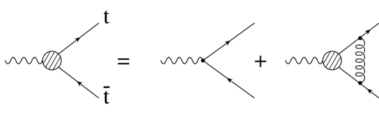
Figure 2: Graphical representation of the Lippmann-Schwinger equations.

A method to see this function appear in a diagrammatical approach in momentum space is as follows: one can express the fact that all gluon exchanges have to be summed (in ladder approximation) in the form of self-consistency equations for the vertex functions $\Gamma_{\cal C}$, with ${\cal C}=\gamma^{\mu}$ or $\gamma^{\mu}\gamma^{5}$ in the case of interest for $e^{+}e^{-}$ annihilation,

$$\Gamma_{\cal C}={\cal C}+\int\!{d^{4}k\over(2\pi)^{4}}\left(-{4\over 3}4\pi\alpha_{\rm s}\right)D_{\mu\nu}(p-k)\gamma^{\mu}S_{\rm F}(k+{q\over 2})\Gamma_{\cal C}(k,q)S_{\rm F}(k-{q\over 2})\gamma^{\nu},$$ (1)

which are also shown in Fig. 2. In the nonrelativistic approximation, neglecting terms of the order $\beta^{2}$, they can essentially be reduced to the integral equations

$${\cal K}_{\rm S}({\rm p},E) = 1+\int{d^{3}k\over(2\pi)^{3}}V({\bf p}-{\bf k}){{\cal K}_{\rm S}({\rm k},E)\over E-{{\bf k}^{2}\over m_{t}}+i\Gamma_{t}}$$ (2)

$${\cal K}_{\rm P}({\rm p},E) = 1+\int{d^{3}k\over(2\pi)^{3}}{{\bf p}\cdot{\bf k}\over{\bf p}^{2}}V({\bf p}-{\bf k}){{\cal K}_{\rm P}({\rm k},E)\over E-{{\bf k}^{2}\over m_{t}}+i\Gamma_{t}}.$$ (3)

The functions ${\cal K}$ in turn are tightly connected to the Green function ${\cal G}$ which solves the Lippmann-Schwinger equation

$$\bigg{[}E-{{\bf p}^{2}\over m_{t}}+i\Gamma_{t}\bigg{]}{\cal G}({\bf p},{\bf x},E)=e^{i{\bf p}\cdot{\bf x}}+\int{d^{3}k\over(2\pi)^{3}}V({\bf p}-{\bf k}){\cal G}({\bf k},{\bf x},E):$$ (4)

expanding ${\cal G}$ in a Taylor series around ${\bf x}=0$ we find

$${\cal G}({\bf p},{\bf x},E)=G({\rm p},E)+{\bf x}\cdot i{\bf p}\,F({\rm p},E)+\ldots$$

with

$$G({\rm p},E)=G_{0}({\rm p},E){\cal K}_{\rm S}({\rm p},E),\qquad F({\rm p},E)=G_{0}({\rm p},E){\cal K}_{\rm P}({\rm p},E)$$ (5)

and

$$G_{0}({\rm p},E)={1\over E-{{\bf p}^{2}\over m_{t}}+i\Gamma_{t}}.$$ (6)

$G$ and $F$ thus are the $S$- and $P$-wave Green functions, respectively. They form the nontrivial dynamical ingredients for the production cross-section which is otherwise completely determined by electroweak coupling constants. For a realistic potential they have to be determined numerically, and it turns out convenient to perform this calculation directly in momentum space using a method introduced in [4].

We will employ the following conventions for the fermion couplings

$$v_{f}=2I^{3}_{f}-4q_{f}\sin^{2}\theta_{\rm W},\qquad a_{f}=2I^{3}_{f}$$ (7)

and the useful abbreviations

$$\begin{array}[]{ll}a_{1}=(q_{e}q_{t}+v_{e}v_{t}d_{Z})^{2}+(a_{e}v_{t}d_{Z})^{2}&a_{2}=2a_{e}v_{t}d_{Z}(q_{e}q_{t}+v_{e}v_{t}d_{Z})\\ a_{3}=2a_{e}a_{t}d_{Z}(q_{e}q_{t}\!+\!2v_{e}v_{t}d_{Z})&a_{4}=2a_{t}d_{Z}(q_{e}q_{t}v_{e}\!+\!(v_{e}^{2}\!+\!a_{e}^{2})v_{t}d_{Z})\\ d_{Z}=\frac{s}{(s-m_{Z}^{2})}\frac{1}{16\sin^{2}\Theta_{W}\cos^{2}\Theta_{W}}.\end{array}$$ (8)

$P_{\pm}$ denotes the longitudinal positron/electron polarization and the variable $\chi$ is defined as

$$\chi={P_{+}-P_{-}\over 1-P_{+}P_{-}}.$$ (9)

With these parameters the differential cross-section for the production of a $t\bar{t}$ pair with a top quark of three-momentum ${\bf p}$ and spin projection $1/2$ on direction n can be written in the form

$$\frac{d^{3}\sigma}{dp^{3}} = \frac{1}{4\pi{\rm p}^{2}}\frac{d\sigma}{d{\rm p}}\Big{(}1+2{\cal A}_{\rm{}_{FB}}({\rm p},E)\cos\vartheta\Big{)}\frac{1+{\bf P}\cdot{\bf n}}{2}$$ (10)

$$\frac{d\sigma}{d{\rm p}} = \frac{3\alpha^{2}}{m_{t}^{4}}\Big{(}1-P_{+}P_{-}\Big{)}\Big{(}a_{1}+\chi a_{2}\Big{)}\cdot\Gamma_{t}\cdot|{\bf p}\cdot G({\rm p},E)|^{2}.$$ (11)

${\cal A}_{\rm{}_{FB}}$ denotes the (momentum dependent) forward-backward asymmetry and P can be interpreted as top quark polarization vector. These quantities are given by

$${\cal A}_{\rm{}_{FB}}({\rm p},E) = -C_{\rm{}_{N}}(\chi)\,\varphi_{\rm{}_{R}}({\rm p},E)$$ (12)

$${\rm P}_{{}_{\parallel}}({\rm p},E) = C_{{}_{\parallel}}^{0}\,+\,C_{{}_{\parallel}}^{1}\cdot\varphi_{\rm{}_{R}}({\rm p},E)\cos\vartheta$$ (13)

$${\rm P}_{\perp}({\rm p},E) = C_{\perp}\cdot\varphi_{\rm{}_{R}}({\rm p},E)\sin\vartheta$$ (14)

$${\rm P}_{\rm{}_{N}}({\rm p},E) = C_{\rm{}_{N}}\cdot\varphi_{\rm{}_{I}}({\rm p},E)\sin\vartheta$$ (15)

with ${\rm P}_{{}_{\parallel},\perp,\rm_{N}}={\bf P}\cdot{\bf n}_{{}_{\parallel},\perp,\rm_{N}}$,

$$C_{{}_{\parallel}}^{0}(\chi) = -\frac{a_{2}+\chi a_{1}}{a_{1}+\chi a_{2}}$$ (16)

$$C_{{}_{\parallel}}^{1}(\chi) = \big{(}1-\chi^{2}\big{)}\frac{a_{2}a_{3}-a_{1}a_{4}}{(a_{1}+\chi a_{2})^{2}}$$ (17)

$$C_{\perp}(\chi) = -\frac{1}{2}\frac{a_{4}+\chi a_{3}}{a_{1}+\chi a_{2}}$$ (18)

$$C_{\rm{}_{N}}(\chi) = \frac{1}{2}\frac{a_{3}+\chi a_{4}}{a_{1}+\chi a_{2}},$$ (19)

$$\varphi({\rm p},E)=\frac{{\rm p}}{m_{t}}\cdot\frac{F^{*}({\rm p},E)}{G^{*}({\rm p},E)}$$ (20)

and $\varphi_{\rm{}_{R}}=\mbox{Re}\,\varphi$, $\varphi_{\rm{}_{I}}=\mbox{Im}\,\varphi$. They have first been derived for polarized beams in [8], apart from P${}_{\rm{}_{N}}$ which has been supplemented in [9]. The forward-backward asymmetry has been calculated first, for unpolarized beams, in [5].

Figure 3: The coefficient functions $C_{x}$ for $\sqrt{s}/2=m_{t}=180$ GeV.

The coefficient functions $C_{x}$ are displayed in figure 3. It is not difficult to see that for small $\beta$ the top quark spin is mainly aligned with the electron beam direction, apart from corrections of order $\beta$ that depend on the production angle $\vartheta$.

However, the size of these ${\cal O}(\beta)$ corrections is not really given by the expressions above, although they are correct in a formal sense. Close to threshold $\beta\sim\alpha_{\rm s}$ and consequently ${\cal O}(\alpha_{\rm s})$ terms might be as large, or put another way, they should be included in the ${\cal O}(\beta)$ analysis.

Some of these QCD corrections are not too difficult to implement because they are universal. The $\gamma t\bar{t}$ and $Zt\bar{t}$ vertex corrections caused by the exchange of transverse gluons for example can be incorporated to the required order by simply multiplying with the following factors [10]:

$$G({\rm p},E) \longrightarrow \Big{(}1-\frac{8\alpha_{\rm s}}{3\pi}\Big{)}G({\rm p},E)$$ (21)

$$F({\rm p},E) \longrightarrow \Big{(}1-\frac{4\alpha_{\rm s}}{3\pi}\Big{)}F({\rm p},E)$$ (22)

resulting in a corresponding modification in the definition of $\varphi({\rm p},E)$. Corrections to the individual top decays can be accounted for by using the 1-loop result for $\Gamma_{t}$ [11].

There is however a type of corrections which is more difficult because it connects the different stages of the production and subsequent decay process. I will call them “rescattering corrections”, the corresponding diagrams are depicted in figure 4 (in principle there is a third diagram with gluon exchange between the two $b$-quarks, which can however be neglected to the required order [9]).

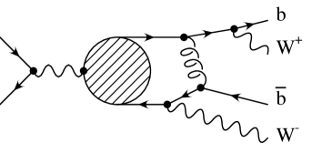
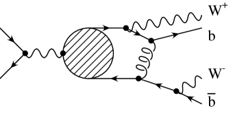
a)	b)

Figure 4: Rescattering diagrams.

Fortunately, their contribution to the total cross-section vanishes [5, 12], but as has first been shown in [5], the contribution to the forward-backward asymmetry does not (although it was found to be small in a numerical study [7]). And there is no a priori argument why they should be irrelevant for the polarization vector, especially for those components which start at order $\beta$, i.e P_⟂ and P${}_{\rm{}_{N}}$. For this reason I will discuss rescattering corrections in the following two sections.

3 Corrections to the differential cross-section

By making use of the nonrelativistic approximation, the calculation of the rescattering corrections to the differential cross-section can essentially be performed along the same line as that of the leading order result. Therefore I will skip that part and only discuss the result. The reader who is interested in the technical aspects should consult [9] or [5].

Defining the two convolution functions

$$\psi_{1}({\rm p},E) = 2\,\mbox{Im}\int\!\frac{d^{3}k}{(2\pi)^{3}}V(|{\bf k}-{\bf p}|)\frac{G({\rm k},E)}{G({\rm p},E)}\frac{\arctan{\frac{|{\bf k}-{\bf p}|}{\Gamma_{t}}}}{|{\bf k}-{\bf p}|}$$ (23)

$$\psi_{2}({\rm p},E) = 2\int\!\frac{d^{3}k}{(2\pi)^{3}}V(|{\bf k}-{\bf p}|)\frac{{\bf p}\cdot({\bf k-p})}{{\rm p}|{\bf k-p}|^{2}}\frac{G({\rm k},E)}{G({\rm p},E)}$$ (24)

$$\times\Big{(}1-\frac{\Gamma_{t}}{|{\bf k}-{\bf p}|}\arctan{\frac{|{\bf k}-{\bf p}|}{\Gamma_{t}}}\Big{)}$$

$$\psi_{\rm{}_{R}}({\rm p},E) = \mbox{Re}\;\psi_{2}({\rm p},E),$$ (25)

the corrected formula for $d^{3}\sigma/dp^{3}$ reads

$$\frac{d^{3}\sigma}{dp^{3}}=\frac{1}{4\pi{\rm p}^{2}}\frac{d\sigma_{\rm Born}}{d{\rm p}}\cdot\Big{(}1+\psi_{1}({\rm p},E)\Big{)}\cdot\Big{(}1+2{\cal A}^{(1)}_{\rm{}_{FB}}({\rm p},E)\cos\vartheta\Big{)}$$ (26)

with

$${\cal A}^{(1)}_{\rm{}_{FB}}({\rm p},E)={\cal A}_{\rm{}_{FB}}({\rm p},E)+\frac{1}{2}\frac{1-2y}{1+2y}\;C_{{}_{\parallel}}^{0}\cdot\psi_{\rm{}_{R}}({\rm p},E)$$ (27)

and $y=m_{W}^{2}/m_{t}^{2}$. Rescattering thus has two effects:

a) E=-3GeV	b) E=5GeV

Figure 5: Shape of the momentum distribution of the top quarks for $E=3$GeV(the position of the would-be 1S resonance) and $E=5$GeV. Dashed line: no rescattering corrections included; solid line: rescattering contribution using the full potential included; dotted line: rescattering contribution included using a pure Coulomb potential with $\alpha_{\rm s}=0.187$.

a) E=-3GeV	b) E=5GeV

Figure 6: Rescattering corrections to the forward-backward asymmetry. Dashed line: $S$-$P$–wave interference contribution; solid line: full result. The little arrows indicate the position of the peak in the momentum distribution.

1. There is a shift in the momentum distribution, as visible in the factor $1+\psi_{1}({\rm p},E)$, which has a simple physical explanation: if $\bar{t}$ decays before $t$, its decay product $\bar{b}$ attracts the top quark and in this way reduces the measured momentum. Figure 5 displays the size of this effect. The dashed lines show the leading order result, the solid and (hardly visible) dotted lines are the corrected curves, with the correction implemented in two different ways: the solid line was calculated using the same potential in the determination of the Green function $G$ and the function $\psi_{1}$; the dotted line was calculated using a pure Coulomb potential in Eq. 23, with the coupling constant fixed to $\alpha_{\rm s}=0.187$ in order to reproduce the solid line. This was done to compare with [5] where a pure Coulomb potential was used as well, but with $\alpha_{\rm s}=\alpha_{\rm s}(\alpha_{\rm s}(M_{Z})m_{t})\approx 0.15$. Of course the scale governing rescattering corrections is of the order of the top momentum ${\rm p}\sim\alpha_{\rm s}(M_{Z})m_{t}$, but when using a fixed coupling constant, its actual value is nevertheless unknown a priori.

2. There is a change in the forward-backward asymmetry which depends on the beam polarization, as can be seen from Fig. 6. The dashed line again shows the uncorrected, the solid line the corrected result. The small arrows indicate the position of the peak in the momentum distribution, i.e. the region which is most relevant. The reason why the corrections were found to be small in [5] is that these authors only considered unpolarized beams.

There are also a few things worth noticing:

The role of $\Gamma_{t}$ as an infrared cut-off is obvious in Eq. 24. For vanishing width the integrand would behave as

$$\frac{V(|{\bf k}-{\bf p}|)}{|{\bf k}-{\bf p}|}\sim\frac{1}{|{\bf k}-{\bf p}|^{3}}$$

for ${\bf k}\sim{\bf p}$, but the factor in brackets weakens this behaviour considerably:

$$\frac{V(|{\bf k}-{\bf p}|)}{|{\bf k}-{\bf p}|}\Big{(}1-\frac{\Gamma_{t}}{|{\bf k}-{\bf p}|}\arctan{\frac{|{\bf k}-{\bf p}|}{\Gamma_{t}}}\Big{)}\sim\frac{1}{3\Gamma_{t}^{2}}\frac{1}{{\rm k}},\qquad|{\bf k}-{\bf p}|\ll\Gamma_{t}.$$

The corrections to the total cross-section indeed vanish because they are proportional to the integral

$$\int\!\frac{d^{3}p}{(2\pi)^{3}}|G({\rm p},E)|^{2}\psi_{1}({\rm p},E)=0.$$

This can be seen by inserting Eq. 23 and interchanging the integration variables ${\bf p}$ and ${\bf k}$.

It is advantageous to solve the Lippmann-Schwinger equations in momentum space because this allows for a relatively easy numerical determination of $\psi_{1}$ and $\psi_{2}$. In the coordinate space approach additional Fourier transformations would be necessary leading to a loss in accuracy.

4 Top quark polarization

The calculation of the rescattering corrections to top quark polarization is more involved than that of the spin-averaged differential cross-section. In the Born-level calulation the quark is essentially treated as a stable particle, the free Green function $G_{0}$ being the only place where its decay enters explicitly through the usage of the complex energy $E+i\Gamma_{t}$. The top quark spin is considered a well defined quantity and thus the appropriate projection operators are used in the derivation of Eq. 10.

This is however no longer possible in the evaluation of the diagram shown in Fig. 4(b). There the top quark appears as a virtual particle only and thus the notion of its polarization is highly questionable. To find a way out one may ask: How will the top quark polarization be measured in a real experiment ?

The answer to this question is known: the experimentalists will use the angular distribution of the leptons from the decay $t\to bl\nu$, because for a free top quark in its rest frame, this is given by

$$\frac{d\Gamma_{t\to bl\nu}({\bf P})}{d\cos\theta}=\frac{1}{2}\Gamma_{t\to bl\nu}\Big{(}1+|{\bf P}|\cos\theta\Big{)}$$

where P denotes the top quark polarization vector and $\theta$ the angle between P and the lepton momentum.

The generalization of this formula to $t\bar{t}$ production in $e^{+}e^{-}$ collisions would be

$$\frac{d^{6}\sigma}{dp^{3}\;dE_{l}\;d\Omega_{l}}=\frac{d^{3}\sigma}{dp^{3}}\cdot\frac{1}{\Gamma_{t}}\frac{d\Gamma_{t\to bl\nu}({\bf P})}{dE_{l}\;d\Omega_{l}}$$ (28)

which expresses the fact that first a top quark with momentum p and polarization P has to be produced, which may then decay semileptonically. Diagram 4(b) however destroys this factorization because the production and decay stages are no longer separated.

Of course the left hand side of Eq. 28 could be calculated nevertheless, at least in principle, however it would lead to a rather complicated result. A method to obtain simpler expressions involving an easier calculation is to consider moments of the lepton spectrum as defined by

$$\langle nl\rangle\equiv\Big{(}\frac{d^{3}\sigma}{dp^{3}}\Big{)}^{-1}\int dE_{l}d\Omega_{l}\frac{d\sigma(e^{+}e^{-}\to bl\nu\bar{b}W^{-})}{dp^{3}\;d\Omega_{p}\;d\Omega_{l}\;dE_{l}}(nl)$$ (29)

or

$$\langle\langle nl\rangle\rangle\equiv\Big{(}\frac{d\sigma}{d{\rm p}}\Big{)}^{-1}\int dE_{l}d\Omega_{l}d\Omega_{p}\frac{d\sigma(e^{+}e^{-}\to bl\nu\bar{b}W^{-})}{d{\rm p}\;d\Omega_{p}\;d\Omega_{l}\;dE_{l}}(nl),$$ (30)

where $l$ is the lepton four-momentum and $n$ may be any convenient four-vector, for example (in the $t\bar{t}$ rest frame)

$$n_{{}_{\parallel}}=(0,{\bf n}_{{}_{\parallel}}) n_{\perp}=(0,{\bf n}_{\perp})$$ (31)

$$n_{\rm{}_{N}}=(0,{\bf n}_{\rm{}_{N}} n_{(0)}=(1,0,0,0).$$ (32)

This method has several advantages [9]:

• it always leads to well-defined, physical, measurable quantities,

• it is far easier than calculating the full multi-differential cross-section because the leptonic phase space can be integrated out completely, even in one of the first steps,

• it still gives us the same information on P, or more exactly, it can be used to define a quantity which is equivalent to P in the absence of rescattering. Neglecting QCD corrections one easily derives from (28)

  $$\langle nl\rangle_{\rm Born}=\mbox{BR}(t\to bl\nu)\cdot\frac{1+2y+3y^{2}}{4(1+2y)}\cdot\Big{[}(n\cdot t)+\frac{m_{t}}{3}(n\cdot P)\Big{]}$$ (33)

  where $t$ and $P$ are four-vectors given by

  $$t=(m_{t},{\bf p})\qquad,\qquad P=(\frac{{\rm p}}{m_{t}}C_{{}_{\parallel}}^{0}\cos\vartheta,{\bf P}).$$ (34)

  The appearance of the 0-component of $P$ is welcome, because if $P$ is to be interpreted as a polarization vector, it has to fulfill the transversality condition $t\cdot P=0$, which indeed it does. Remember that we are working in the $t\bar{t}$ rest frame instead of the $t$ rest frame (the corresponding change in P is of the order $\beta^{2}$ and thus does not appear here).

Rescattering modifies equation (33), the corrected expression reads

$$\langle nl\rangle = \mbox{BR}(t\to bl\nu)\cdot\frac{1+2y+3y^{2}}{4(1+2y)}$$ (35)

$$\cdot\Big{[}(n\cdot t)(1+\varepsilon)+\frac{m_{t}}{3}(n\cdot P+n\cdot\delta P)\Big{]}$$

with

$$\varepsilon = \frac{y(1-y)}{(1+2y)(1+2y+3y^{2})}C_{{}_{\parallel}}^{0}\psi_{\rm R}({\rm p},E)\cos\vartheta$$ (36)

$$\delta{\rm P}_{{}_{\parallel}} = \Bigg{[}\frac{2+3y-5y^{2}-12y^{3}}{(1+2y)(1+2y+3y^{2})}-\frac{1-2y}{1+2y}(C_{{}_{\parallel}}^{0})^{2}\Bigg{]}\psi_{\rm{}_{R}}({\rm p},E)\cos\vartheta$$ (37)

$$+\frac{1-4y+3y^{2}}{4(1+2y+3y^{2})}(1-3\cos^{2}\vartheta)C_{{}_{\parallel}}^{0}\psi_{3}({\rm p},E)$$

$$\delta{\rm P}_{\perp} = \frac{3(1-3y^{2})}{2(1+2y+3y^{2})}\psi_{\rm{}_{R}}({\rm p},E)\sin\vartheta$$ (38)

$$-\frac{3(1-4y+3y^{2})}{8(1+2y+3y^{2})}C_{{}_{\parallel}}^{0}\psi_{3}({\rm p},E)\sin 2\vartheta$$

$$\delta{\rm P}_{\rm{}_{N}} = 0,\qquad\delta{\rm P}_{0}=0.$$ (39)

The new function $\psi_{3}$ is defined as

$$\psi_{3}({\rm p},E) = \mbox{Im}\int\!\!\frac{d^{3}k}{(2\pi)^{3}}V(|{\bf k}-{\bf p}|)\frac{G({\rm k},E)}{G({\rm p},E)}\frac{\arctan\frac{|{\bf k}-{\bf p}|}{\Gamma_{t}}}{|{\bf k}-{\bf p}|}$$ (40)

$$\times\Bigg{[}3\Big{(}\frac{{\bf p\cdot(k-p)}}{{\rm p}|{\bf k}-{\bf p}|}\Big{)}^{2}-1\Bigg{]}$$

and its presence destroys the otherwise nice similarity between $P$ and $\delta P$. Numerically its contribution is however negligible for realistic top quark masses. The same applies to $\varepsilon$ so that at least in practice the form of the Born-level result is recovered. One should note that there was no a priori reason to expect this form to remain the same.

a) E=-3GeV	b) E=5GeV

Figure 7: Subleading part of the longitudinal component of the polarization vector P${}_{{}_{\parallel}}$ for $\vartheta=0$. The solid line shows the complete result for unpolarized beams, the dotted line the $S$-$P$–interference contribution. The dash-dotted line shows the complete result for fully polarized beams, in which case the $S$-$P$–wave contribution vanishes. The arrows indicate the position of the peak in the momentum distribution.

a) E=-3GeV	b) E=5GeV

Figure 8: Transverse component of the polarization vector P_⟂ for $\vartheta=\pi/2$. The solid and dotted lines correspond to unpolarized beams, the dash-dotted and dotted lines to fully polarized beams. The solid and dash-dotted curves show the full result, the dashed and dotted the $S$-$P$–interference contribution. The arrows indicate the position of the peak in the momentum distribution.

In addition I should mention that $\psi_{1}$, $\psi_{2}$ and $\psi_{3}$ could be interpreted as additional $S$-, $P$- and $D$-wave contributions, a viewpoint motiviated by the way they are defined and the way they enter the expressions.

Figures 7 and 8 show the predictions for the subleading term of the longitudinal polarization and for the transverse part, respectively. The solid and dash-dotted lines correspond to the full result for unpolarized/fully polarized beams, the dashed and dotted lines to the ${\cal O}(\beta)$ term only. It is quite evident that rescattering has a strong influence on the result, which is due to the fact that the ${\cal O}(\beta)$-terms are suppressed by ratios of electroweak couplings appearing in the coefficients $C_{{}_{\parallel}}^{1}$ and $C_{\perp}$. $\varphi_{\rm{}_{R}}$ and $\psi_{\rm{}_{R}}$ are of comparable size as they should be because $\beta\sim\alpha_{\rm s}$.

5 Summary and conclusions

In this paper I have discussed recent results on observables in top quark pair production near threshold at $e^{+}e^{-}$ colliders. I have sketched the calculational procedure used to derive the predictions for the differential cross-section and top quark polarization for arbitrary beam polarization which are correct up to terms of the order ${\rm p}^{2}/m_{t}^{2}$ because they also include the rescattering corrections. The method of moments proved to be a very useful tool, which could of course also be used for other production mechanisms or far above threshold.

It turned out that rescattering corrections are not generically small and are indeed required for a consistent prediction of the components of the top quark polarization vector lying in the production plane. They are of minor importance for the forward-backward asymmetry but might nevertheless be visible in precision studies, especially if polarized beams are used. An important result was that there are no corrections to the normal polarization. This component is of special interest because it is the place where non-standard CP violating interactions would manifest themselves. In connection with the leading term of P${}_{{}_{\parallel}}$, which can be measured by averaging over the top direction, i.e. via $\langle\langle n_{{}_{\parallel}}\cdot P\rangle\rangle$, it provides an opportunity to determine the top quark couplings $a_{1}\ldots a_{4}$.

I would like to express my gratitude to the organizers of the XXXVI Cracow School of Theoretical Physics, especially M. Jeżabek, for their invitation and for providing such a nice atmosphere. I would also like to thank J.H. Kühn for carefully reading the manuscript and giving useful advice.

References

- [1] V.S. Fadin and V.A. Khoze, Sov. J. Nucl. Phys. 48 (1988) 309; JETP Lett. 46 (1987) 525.
- [2] M.J. Strassler and M.E. Peskin, Phys. Rev. D 43 (1991) 1500
- [3] Y. Sumino, K. Fujii, K. Hagiwara, H. Murayama and C.-K. Ng, Phys. Rev. D 47 (1993) 56.
- [4] M. Jeżabek, J.H. Kühn and T. Teubner, Z. Phys. C 56 (1992) 653.
-
[5]
Y. Sumino, PhD thesis, University of Tokyo 1993 (unpublished);
H. Murayama and Y. Sumino, Phys. Rev. D 47 (1993) 82. - [6] M. Jeżabek and T. Teubner, Z. Phys. C 59 (1993) 669.
- [7] K. Fujii, T. Matsui and Y. Sumino, Phys. Rev. D 50 (1994) 4341.
- [8] R. Harlander, M. Jeżabek, J.H. Kühn and T. Teubner, Phys. Lett. B 346 (1995) 137.
- [9] R. Harlander, M. Jeżabek, J.H. Kühn and M. Peter, Karlsruhe Preprint TTP95-48, hep-ph/9604328; to be published in Z. Phys. C.
-
[10]
R. Barbieri, R. Gatto, R. Kögerler and Z. Kunszt, Phys. Lett.
57B (1975) 455,
J.H. Kühn and P. Zerwas, Phys. Reports 167 (1988) 321. - [11] M. Jeżabek and J.H. Kühn, Nucl. Phys. B 314 (1989) 1.
- [12] K. Melnikov and O. Yakovlev, Phys. Lett. B 324 (1994) 217.