Analysis of Low-$x$ Gluon Density from the $F_{2}$ Scaling Violations

M. B. Gay Ducati ^∗
and
Victor P. B. Gonçalves ^∗∗

Instituto de Física, Univ. Federal do Rio Grande do Sul
Caixa Postal 15051, 91501-970 Porto Alegre, RS, BRAZIL

Abstract: We present an analysis of the current methods of approximate determination of the gluon density $G(x,Q^{2})$ at low-$x$ from the scaling violations of the proton structure function $F_{2}(x,Q^{2})$. The gluon density is obtained from DGLAP equation by expansion at distinct points of expansion. We show that the different results given by the proposed methods can be obtained from one new expression considering the adequate points of expansion. It is shown in which case the approximate determination of $G(x,Q^{2})$ is reasonable.

PACS numbers: 12.38.Aw; 12.38.Bx; 13.90.+i;

Key-words: Small $x$ QCD; Perturbative calculations; Gluon density.

1 Introduction

Deep Inelastic Scattering (DIS)[1, 2] of electrons on protons provides the classical test of the Quantum Chromodynamics (QCD)[3, 2] at short distances. A complete knowledge of the nucleon structure (parton picture of hadrons), including the gluon density, is fundamental for the design of future proton collider experiments, but more immediate interest in the gluon density centres on the main role it plays for physics at low $x$ and moderate $Q^{2}$. With the advent of HERA, we are working in a new kinematical region both in $Q^{2}$ and $x$. Whereas at large $Q^{2}$ the logarithmic scaling violations predicted by QCD are expected, the direction towards small $x$ leads to a new kinematical region, where new dynamical effects are expected to occur at a significant level.

The standard perturbative QCD framework predicts that at a regime of low values of the Bjorken variable $x$ ($x\approx 10^{-4}$) and large values of $Q^{2}$, a nucleon consists predominantly of the sea quarks and gluons. The gluons couple only through the strong interaction, consequently the gluons are not directly probed in the DIS, only contributing indirectly via the $g\rightarrow q\overline{q}$ transition. Therefore, its distribution is not so well determined as those of the quarks.

Recently, a direct determination of the gluon density was performed in the kinematical region $x>10^{-3}$ [4]. A leading order determination of the gluon density in the proton was performed by measuring multi-jet events from boson-gluon fusion in deep-inelastic scattering with the detector H1 at the electron-proton collider HERA. The data agree with the dramatic rise of gluon density with decreasing $x$ predicted by the traditional analysis of $F_{2}(x,Q^{2})$ [5, 6]. These analysis have performed next-to-leading order (NLO) QCD fits based on the Altarelli-Parisi (DGLAP)[7] evolution equations of the parton densities. The initial densities should be determined by the experiment at some scale $Q^{2}=Q_{0}^{2}$. The basic procedure is to parameterize the $x$ dependence at some low $Q_{0}^{2}$, but where perturbative QCD should be still applicable, and then evolve up in $Q^{2}$ using NLO DGLAP equations to obtain the parton densities at all values of $x$ and $Q^{2}$ of the data. The input parameters are then determined by a global fit to the data.

The parton densities are well determined for $x>0.5$, where there are many different types of high-precision constraints on the individual parton distributions. The exception is the gluon density which is mainly constrained by (i) the momentum sum rule, (ii) prompt photon production and (iii) the scaling violations of $F_{2}$. On the other hand at small $x$ $(x\leq 10^{-3})$ we have only the measurement of the structure function $F_{2}(x,Q^{2})$, and many different partonic descriptions at small $x$, for example, DGLAP[7] and BFKL[8]. Therefore it is important to obtain more information in this region, mainly of the gluon density, which is the dominant parton at small $x$.

Using the fact that quark densities can be neglected and that the non-singlet contribution $F_{2}^{NS}$ can be ignored safely at low $x$ in the DGLAP equations, the equation for $F_{2}$ becomes, for four flavours

$$\frac{dF_{2}(x,Q^{2})}{dlogQ^{2}}=\frac{10\alpha_{s}}{9\pi}\int_{x}^{1}dx^{\prime}P_{qg}(x^{\prime})\frac{x}{x^{\prime}}g\left(\frac{x}{x^{\prime}},Q^{2}\right)\,\,\,,$$ (1)

where $g(x,Q^{2})$ is the gluon density, $xg(x,Q^{2})=G(x,Q^{2})$ is the gluon density momentum, $\alpha_{s}=\alpha_{s}(Q^{2})$ is the strong coupling constant and the splitting function $P_{qg}(x^{\prime})$ gives the probability of finding a quark inside a gluon with momentum $x^{\prime}$ of the gluon.

In LO (leading order)

$$P_{qg}(x^{\prime})=\frac{1}{2}[x^{\prime 2}+(1-x^{\prime})^{2}]\,\,\,.$$ (2)

Substituting $x^{\prime}=1-z$ we can write

$$\frac{dF_{2}(x,Q^{2})}{dlogQ^{2}}=\frac{10\alpha_{s}}{9\pi}\int_{0}^{1-x}dzP_{qg}(1-z)G\left(\frac{x}{1-z},Q^{2}\right)\,\,\,.$$ (3)

Moreover, in LO $P_{qg}(z)=P_{qg}(1-z)$, then

$$\frac{dF_{2}(x,Q^{2})}{dlogQ^{2}}=\frac{10\alpha_{s}}{9\pi}\int_{0}^{1-x}dzP_{qg}(z)G\left(\frac{x}{1-z},Q^{2}\right)\,\,\,.$$ (4)

This equation describes the evolution of the proton structure function $F_{2}(x,Q^{2})$ in LO at small $x$. From experiments one can measure the structure function and then determine its derivative $\frac{dF_{2}(x,Q^{2})}{dlogQ^{2}}$. Some methods [9, 10] were proposed in the literature to isolate the gluon density by its expansion inside expression (4), but have different results for $G(x,Q^{2})$. We demonstrate here that one of the methods is not totally correct and that, when it is corrected, the results of both methods can be obtained by using different points of expansion from one general expression. This article will be organized as follows. In sect. 2 a revision of the methods proposed in the literature is made. We show that one of these methods is not totally correct and we present a modification. In sect. 3 we propose a general expression for the approximate determination of the gluon density and determine the appropriate points of expansion using data for $\frac{dF_{2}(x,Q^{2})}{dlogQ^{2}}$, obtained by H1[11], Zeus[12] and also for a screnning model [13] recently appeared in the literature. Finally, in the sect. 4, we present our conclusions.

2 Analysis of Approximative Methods

The methods of approximate determination of the gluon density are based on the simplification of the convolution $P_{qg}\bigotimes g$ (eq. (1)) by the expansion of the gluon density. The result is the gluon density $G(k.x)$ proportional to the derivative of $F_{2}(x,Q^{2})$, where the constant $k$ is associated to the choice of a point of expansion and $x=x_{B}$. In DIS we do not probe the gluon directly, but instead via the process $g\rightarrow q\overline{q}$. The longitudinal fraction $x_{g}$ of the proton’s momentum that is carried by the gluon is therefore sampled over an interval bounded below by the Bjorken $x_{B}$ variable $x_{B}\equiv\frac{Q^{2}}{2p.q}$, where as usual $p$ and $q$ are the four momenta of the incoming proton and virtual photon respectively and $Q^{2}\equiv-q^{2}$. Therefore, the choice of the point of expansion, and consequently of $k$, is associated with the relation between $x_{g}$ and $x_{B}$. We discuss the methods of approximate determination of gluon density proposed in the literature below.

2.1 Prytz’s Approach

Substituting $P_{qg}(x^{\prime})$ in the expression (4) and then expanding the gluon distribution around $z=\frac{1}{2}$, one gets [9]

$$\frac{dF_{2}(x,Q^{2})}{dlogQ^{2}} \approx \frac{5\alpha_{s}}{9\pi}G(2x)\int_{0}^{1-x}dz[(1-z)^{2}+z^{2}]+$$ (5)

$$+\frac{5\alpha_{s}}{9\pi}\frac{dG(z=\frac{1}{2})}{dz}\int_{0}^{1-x}dz[(1-z)^{2}+z^{2}](z-\frac{1}{2})\,\,\,.$$

Approximating the upper integration limit $1-x\approx 1$ we can write

$$\frac{dF_{2}(x,Q^{2})}{dlogQ^{2}} \approx \frac{5\alpha_{s}}{9\pi}G(2x)\int_{0}^{1}dz[(1-z)^{2}+z^{2}]$$ (6)

$$\approx \frac{10\alpha_{s}}{27\pi}G(2x)\,\,\,.$$ (7)

Therefore the gluon distribution can be expressed by

$$G(2x) \approx \frac{27\pi}{10\alpha_{s}}\frac{dF_{2}(x,Q^{2})}{dlogQ^{2}}\,\,\,.$$ (8)

The author of ref. [9] claims that this relation is valid within 20% of accuracy, by taking into account many uncertainties: experimental measurement of the $Q^{2}$-dependence of $F_{2}$, the value of $\alpha_{s}$ and the discarding of any typical low-$x$ effects calculated beyond the DGLAP approximation, for example recombination effects[14]. Estimates of gluon density [4] have demonstrated that this approximation agrees with the gluon density obtained with other indirect determinations made by H1 and Zeus Collaborations.

2.2 Bora’s et al. Approach

A different method is based in expansion of gluon distribution around $z=0$. Substituting the result in the expression (4) one gets [10]

$$\frac{dF_{2}(x,Q^{2})}{dlogQ^{2}}\approx\frac{5\alpha_{s}}{9\pi}G(x)\left\{\frac{2(1-x)^{3}}{3}-(1-x)^{2}+(1-x)\right\}+$$

$$+\frac{5\alpha_{s}}{9\pi}\left\{\frac{(1-x)^{2}}{2}-\frac{2(1-x)^{3}}{3}+\frac{(1-x)^{4}}{2}\right\}\left\{x\frac{dG}{dx}\right\}\,\,\,.$$ (9)

Therefore

$$\frac{dF_{2}(x,Q^{2})}{dlogQ^{2}}\approx\frac{5\alpha_{s}}{9\pi}A(x)\left\{G(x)+\frac{B(x)}{A(x)}x\frac{dG}{dx}\right\}\,\,\,.$$ (10)

where

$$A(x)=\frac{2(1-x)^{3}}{3}-(1-x)^{2}+(1-x)\,\,\,,$$ (11)

and

$$B(x)=\frac{(1-x)^{2}}{2}-\frac{2(1-x)^{3}}{3}+\frac{(1-x)^{4}}{2}\,\,\,.$$ (12)

Bora et al. [10] claim that this expression can be approximated by

$$\frac{dF_{2}(x,Q^{2})}{dlogQ^{2}}\approx\frac{5\alpha_{s}}{9\pi}\frac{[A(x)+B(x)]^{2}}{A(x)+2B(x)}G\left(x+\frac{B(x)}{A(x)+B(x)}x\right)$$ (13)

$$\Rightarrow G\left(x+\frac{B(x)}{A(x)+B(x)}x\right)\approx\frac{9\pi}{5\alpha_{s}}\frac{A(x)+2B(x)}{[A(x)+B(x)]^{2}}\frac{dF_{2}(x,Q^{2})}{dlogQ^{2}}\,\,\,.$$ (14)

In the limit $x\rightarrow 0$ the last equation becomes

$$G\left(\frac{4}{3}x\right)\approx\frac{9\pi}{5\alpha_{s}}\frac{4}{3}\frac{dF_{2}(x,Q^{2})}{dlogQ^{2}}\,\,\,.$$ (15)

In figure (1) we compare the results of $\frac{dF_{2}(x,Q^{2})}{dlogQ^{2}}$ for the approximate relations of Prytz (7), Bora et al.(13) and the complete expression (4) using the gluon distribution GRV94(LO) [6]. In our calculations the value of $\alpha_{s}$ is obtained at $\Lambda_{\overline{MS}}^{(4)}=0.232GeV^{2}$. The figure shows that Prytz approximation is more accurate.

The result (15) differs from Prytz result (8). Bora et al. explain that the difference arises because they have retained the $x$ dependence in the upper limit of integration in equation (4) after the expansion of the gluon density. In order to show this is not the case, we have computed the expression (5) without approximation in the upper integration limit. One gets

$$\frac{dF_{2}(x,Q^{2})}{dlogQ^{2}} \approx \frac{5\alpha_{s}}{9\pi}[(1-x)-(1-x)^{2}+\frac{2}{3}(1-x)^{3}]\left\{G(2x)+\frac{dG(z=\frac{1}{2})}{dz}\right.$$ (16)

$$\left.\left[\frac{\frac{1}{2}(1-x)^{2}-\frac{2}{3}(1-x)^{3}+\frac{1}{2}(1-x)^{4}}{(1-x)-(1-x)^{2}+\frac{2}{3}(1-x)^{3}}-\frac{1}{2}\right]\right\}\,\,\,.$$

Consequently,

$$\frac{dF_{2}(x,Q^{2})}{dlogQ^{2}} \approx \frac{5\alpha_{s}}{9\pi}[(1-x)-(1-x)^{2}+\frac{2}{3}(1-x)^{3}].$$ (17)

$$.G\left(x+\frac{\frac{1}{2}(1-x)-\frac{2}{3}(1-x)^{2}+\frac{1}{2}(1-x)^{3}}{1-(1-x)+\frac{2}{3}(1-x)^{2}}x\right)\,\,\,.$$

In the limit $x\rightarrow 0$, this equation becomes

$$\frac{dF_{2}(x,Q^{2})}{dlogQ^{2}} \approx \frac{5\alpha_{s}}{9\pi}\frac{2}{3}G(2x)$$ (18)

$$\Rightarrow G(2x) \approx \frac{9\pi}{5\alpha_{s}}\frac{dF_{2}(x,Q^{2})}{dlogQ^{2}}\,\,\,.$$ (19)

This result is identical to the Prytz one, demonstrating that Bora’s argument is not correct.

The Bora’s method requires that

$$\frac{[B(x)]^{2}}{A(x)[A(x)+2B(x)]}\approx 0\,\,\,,$$ (20)

$$\frac{A(x)+B(x)}{A(x)+2B(x)}\approx 1\,\,\,.$$ (21)

In figure (2) we present the behaviour of these expressions at small $x$. We immediately see that for small $x$ these approximations are not valid. Consequently the Bora approximation is not valid in this $x$ range.

The more adequate approximation of expression (10) is

$$\frac{dF_{2}(x,Q^{2})}{dlogQ^{2}} \approx \frac{5\alpha_{s}}{9\pi}A(x)G\left(x+\frac{B(x)}{A(x)}x\right)\,\,\,.$$ (22)

In the limit $x\rightarrow 0$ , the equation becomes

$$\frac{dF_{2}(x,Q^{2})}{dlogQ^{2}} \approx \frac{5\alpha_{s}}{9\pi}\frac{2}{3}G\left(\frac{3}{2}x\right)\,\,\,.$$ (23)

In figure (3) we presented the behaviour of Prytz (7) and Bora (13) results and one obtained from expression (23), called Bora corrected. The expression (23) also differs from the expression of Prytz (7). This is due to the election of a different point of expansion of the gluon density in both cases. In the next section we demonstrate that both results can be obtained from a general equation by choosing the adequate point of expansion.

3 Expansion at an arbitrary point of expansion

Using the expansion of the gluon distribution $G\left(\frac{x}{1-z}\right)$ at an arbitrary $z=\alpha$ and retaining terms only up to the first derivative in the expansion, we get

$$\frac{dF_{2}(x,Q^{2})}{dlogQ^{2}}\approx\frac{5\alpha_{s}}{9\pi}\left\{\frac{2}{3}(1-x)^{3}-(1-x)^{2}+(1-x)\right\}.$$

$$.G\left[\frac{x}{1-\alpha}\left(1-\alpha+\frac{\frac{1}{2}(1-x)^{3}-\frac{2}{3}(1-x)^{2}+\frac{1}{2}(1-x)}{\frac{2}{3}(1-x)^{2}-(1-x)+1}\right)\right]\,\,\,.$$ (24)

In the limit $x\rightarrow 0$ , the equation becomes

$$\frac{dF_{2}(x,Q^{2})}{dlogQ^{2}} \approx \frac{5\alpha_{s}}{9\pi}\frac{2}{3}G\left[\frac{x}{1-\alpha}\left(\frac{3}{2}-\alpha\right)\right]\,\,\,.$$ (25)

When the points $\alpha=\frac{1}{2}$ and $\alpha=0$ are used, we get

$$\frac{dF_{2}(x,Q^{2})}{dlogQ^{2}} \approx \frac{5\alpha_{s}}{9\pi}\frac{2}{3}G(2x)\,\,\,,$$ (26)

$$\frac{dF_{2}(x,Q^{2})}{dlogQ^{2}} \approx \frac{5\alpha_{s}}{9\pi}\frac{2}{3}G\left(\frac{3}{2}x\right)\,\,\,.$$ (27)

Therefore the equation (24) can be reduced to Prytz (7) and Bora corrected (23), in their respective points of expansion.

The gluon distribution for a point of expansion $\alpha<1$ can be expressed by

$$G\left[\frac{x}{1-\alpha}\left(\frac{3}{2}-\alpha\right)\right] \approx \frac{9\pi}{5\alpha_{s}}\frac{3}{2}\frac{dF_{2}(x,Q^{2})}{dlogQ^{2}}\,\,\,.$$ (28)

In figure (4) we present the results of $\frac{dF_{2}(x,Q^{2})}{dlogQ^{2}}$ at some points of expansion $\alpha$ using the gluon distribution GRV94(LO), which fits better the recent data of H1 Collaboration [15]. At the current data of $\frac{dF_{2}(x,Q^{2})}{dlogQ^{2}}$ the points $\alpha\geq 0.5$ are favoured. This means that in this kinematical region the longitudinal momentum of the gluon $x_{g}$ is more than twice the value of the longitudinal momentum of the probed quark (or antiquark) in DIS.

One can ask if the approximative determination of the gluon density from $F_{2}(x,Q^{2})$ scaling violations can indicate the presence of new effects at low-$x$, for example, recombination. In figure (5) we present the behaviour obtained using (28) for distinct points of expansion and $\frac{dF_{2}(x,Q^{2})}{dlogQ^{2}}$ data calculated using the Glauber(Mueller) approach[13]. This approach includes shadowing corrections and $\frac{dF_{2}(x,Q^{2})}{dlogQ^{2}}$ can be calculated using the total cross section of the gluon pair with the nucleon in the eikonal approach.

We can conclude that, when compared with the behaviour of GRV94(LO), the screnning can be cancealed for some values of $\alpha$ and that the better choices (with greater sensitivity to screnning) are in the range $0.5\leq\alpha<0.8$. This conclusion agrees with that of Ryskin et al. [18] that estimate the value of the longitudinal gluon momenta $x_{g}$ in approximately 3 times larger than the Bjorken $x_{B}$, that corresponds to the expansion at $\alpha=0.75$.

4 Conclusions

The gluon is by far the dominant parton in the small $x$ regime. Its distribution is not well determined as those of the quark, and there are several methods proposed in the literature in order to determine it in different regions of $x$. More recently, new methods [9, 10, 16, 17] also based on the dominant behaviour of the gluon distribution at small-$x$ were proposed.

In this work we discuss the approximative determination of the gluon density at low-$x$ from $F_{2}(x,Q^{2})$ scaling violations [9, 10]. We demonstrate that one of these methods is not correct. Moreover we proposed one general expression for approximative determination of the gluon density at arbitrary point of expansion of $G\left(\frac{x}{1-z}\right)$. Using data of H1 and Zeus Collaborations [11, 12] and results obtained from Glauber (Mueller) approach [13] that includes shadowing corrections, we conclude that the more suitable points of expansion (with greater sensitivity to screnning) are in the range $0.5\leq\alpha<0.8$. This conclusion agrees with recent results obtained by Ryskin et al.[18].

The approximative determination of the gluon density obtained in this work was developed in the DGLAP framework. Consequently the approximation is valid in the DGLAP limit, which surely breaks down at sufficiently small $x$. When $\alpha_{s}ln\frac{1}{x}\approx 1$ we should resum also the $\alpha_{s}ln\frac{1}{x}$ contributions. In LO, $(\alpha_{s}ln\frac{1}{x})^{n}$ resummation is acomplished by the BFKL equation [8]. Therefore, a rigorous determination of the transition region to small-$x$ dynamics is very important in order to isolate correctly the gluon distribution.

Figure Captions

Fig. 1: Results of the $\frac{dF_{2}(x,Q^{2})}{dlogQ^{2}}$ obtained from relations of Prytz (7), Bora (13) and (4), using GRV94(LO)[6]. Data from H1 [11] and Zeus[12] at $Q^{2}=20$ $GeV^{2}$.

Fig. 2: Behaviour of approximations used by Bora et al. [10].

Fig. 3: Same as for figure (1), including results of equation (23) presented for $Q^{2}=20$ $GeV^{2}$.

Fig. 4: Behaviour of $\frac{dF_{2}(x,Q^{2})}{dlogQ^{2}}$ at several points of expansion $\alpha$. Also plotted the behaviour obtained using GRV94(LO) and the expression (4) at $Q^{2}=20$ $GeV^{2}$.

Fig. 5: Gluon distributions obtained of (28) using $\frac{dF_{2}(x,Q^{2})}{dlogQ^{2}}$ with screnning[13]. Also shown the gluon distribution of GRV94(LO).

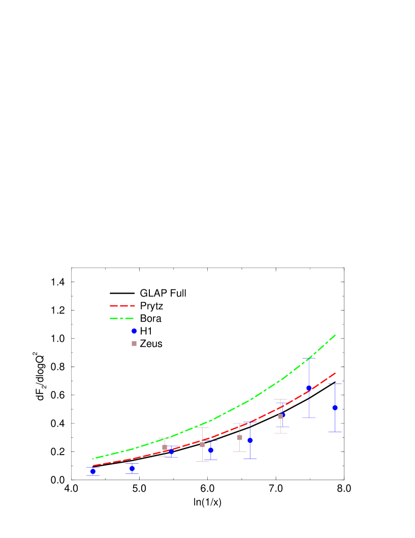
Figure 1:

Figure 2:

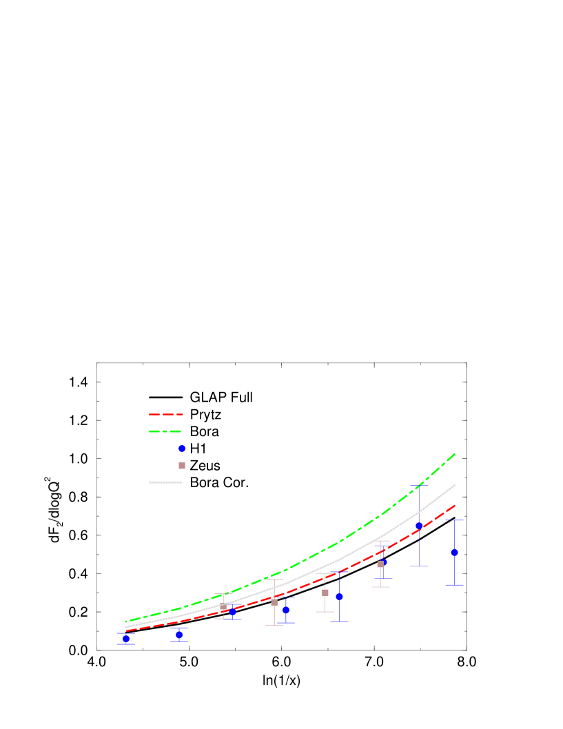
Figure 3:

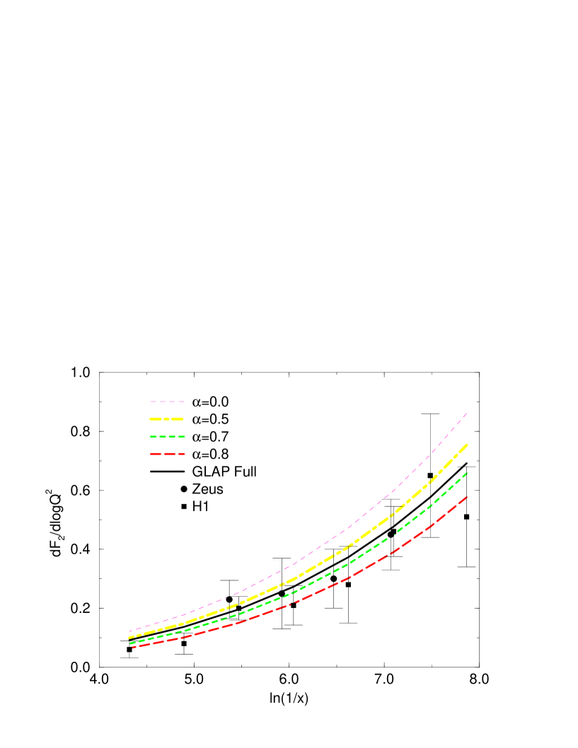
Figure 4:

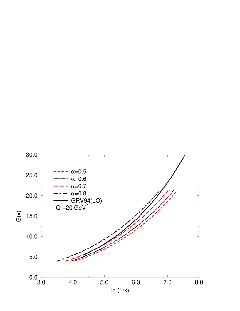
Figure 5:

References

- [1] C. A. Garcia Canal, M. B. Gay Ducati, J.A.M. Simões. Notes on Deep Inelastic Scattering. Strasbourg: Centre de Recherches Nucleaires et Université Louis Pasteur,1980. (Series des Cours et Conferences sur la Physique des Hautes Energies, 15).
- [2] R.G. Roberts. The Structure of the Proton. Cambridge University Press (1990).
- [3] E. Reya. Phys.Rep. 69C (1981) 195; G. Altarelli. Phys.Rep. 81C (1982) 1.
- [4] S. Aid et al.. Nucl. Phys. B449 (1995) 3.
- [5] A.D. Martin, R.G. Roberts and W.J. Stirling. Phys. Lett 354 (1995) 155.
- [6] M. Gluck, E. Reya and A. Vogt. Z. Phys. C67 (1995) 433.
- [7] Yu. L. Dokshitzer. Sov. Phys. JETP 46 (1977) 641; G. Altarelli and G. Parisi. Nucl. Phys. B126 (1977) 298; V. N. Gribov and L.N. Lipatov. Sov. J. Nucl. Phys 28 (1978) 822.
- [8] E.A. Kuraev, L.N. Lipatov and V.S. Fadin. Phys. Lett B60 (1975) 50; Sov. Phys. JETP 44 (1976) 443; Sov. Phys. JETP 45 (1977) 199; Ya. Balitsky and L.N. Lipatov. Sov. J. Nucl. Phys. 28 (1978) 822.
- [9] K. Prytz. Phys. Lett. B 311 (1993) 286; Phys. Lett. B 332 (1994) 393.
- [10] K. Bora and D.K. Choudhury. Phys. Lett. B354 (1995) 151.
- [11] S. Aid et al.. Phys. Lett. B354 (1995) 494.
- [12] M. Derrick et al. . Phys. Lett. B345 (1995) 576.
- [13] A. L. Ayala, M. B. Gay Ducati and E. M. Levin. QCD Evolution of the Gluon Density in a Nucleus. CBPF - NF - 020/96, hep-ph 9604383, April 1996.
- [14] L. V. Gribov, E. M. Levin and M. G. Ryskin. Phys.Rep. 100 (1983) 1.
- [15] S. Aid et al.. Nucl. Phys. B470 (1996) 3.
- [16] A.M. Cooper-Sarkar et al.. Z. Phys. C39 (1988) 281.
- [17] A. Vogt . Constraining the Proton’s Gluon Density by Inclusive Charm Electroproduction at HERA. hep-ph/9601352, January 1996.
- [18] M. G. Ryskin, A. G. Shuvaev and Yu. M. Shabelski. Z. Phys. C (in press). hep-ph/9512297, December 1995.