SUMMARY

Some of the new experimental results and theoretical developments presented at the Workshop on Deep Inelastic Scattering and Related Phenomena are reviewed.

1 Introduction

The present series of Workshops on deep inelastic scattering and related high-energy processes began in Durham in 1993. At that time results from the HERA $ep$ collider were beginning to appear, and a forum where experimentalists and theorists could get together to discuss these and other related measurements seemed appropriate. The meeting was a resounding success. The quality and quantity of the physics, together with the enthusiasm of the participants, all pointed towards the establishment of a ‘deep inelastic scattering’ workshop as an annual event. The Eilat (1994) and Paris (1995) meetings confirmed the Workshop as a truly international meeting, and one of the most important in the high energy physics calendar. This tradition has been continued in Rome, with a record number of participants and a wealth of interesting physics.

Although HERA provided the original motivation, one of the keys to the success of the DIS Workshops is the way they draw together the whole deep inelastic scattering community, with fixed-target experiments playing an equally important role. The hadron collider community has also been well represented, illustrating the complementarity of lepton-hadron and hadron-hadron collisions in providing information on hadron structure.

There have been four main strands to the physics discussed at this Workshop: (i) investigating the parton structure of the proton and photon as revealed in high-energy lepton-hadron and photon-hadron collisions respectively; (ii) understanding the origin of those events which are both deeply inelastic and diffractive; (iii) studying detailed QCD dynamics by means of particular hadronic final states (jets, heavy flavours, …); and (iv) unravelling the spin structure of the nucleon by means of polarized deep inelastic scattering experiments. In this brief review I will attempt to highlight some of the new results in these different areas, together with their theoretical implications. The choice is necessarily restricted (lack of space and personal expertise being the main constraints) and does not come close to doing justice to all the interesting physics which has been presented and discussed. Nevertheless, I hope it will give a flavour of what is without question one of the most important frontiers of particle physics today.

2 Proton structure

The traditional method of obtaining information on the parton structure of the nucleon is through measurements of deep inelastic structure functions. The key variables (for example, for the process ${\rm e}^{-}(k)+{\rm p}(p)\to{\rm e}^{-}(k^{\prime}=k-q)+X$) are $x$ and $Q^{2}$, where

$$Q^{2}=-q^{2}=-(k-k^{\prime})^{2}\;,\qquad x=Q^{2}/2p\cdot q\;.$$ (1)

Structure functions ${\cal F}_{i}(x,Q^{2})$ are then obtained from the differential scattering cross section, $d^{2}\sigma/dxdQ^{2}$. The main advance in recent years has been the dramatic increase in the range of $x$ and $Q^{2}$ covered by experiment. With improvements in luminosity and detectors, HERA has been able to measure $F_{2}^{ep}$ down to $x\sim 10^{-5}$. At the same time, the $Q^{2}$ range has been extended both at the upper and lower ends. For the former, this leads to an increase in quark substructure limits (see Section 2.6) and tests of perturbative QCD (pQCD) evolution. Data at low $Q^{2}$ are important for providing a bridge to the fixed-target data, and also for understanding the perturbative/nonperturbative transition. The region covered by the most recent HERA and fixed-target data is illustrated in Fig. 1.

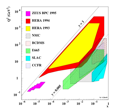
Figure 1: $x,Q^{2}$ phase space covered by various recent DIS experiments.

2.1 New structure function measurements

Two significant improvements have been reported at this Workshop $\!{}^{{\bf?},{\bf?}}$. The 1994 HERA $F_{2}$ data now overlap with the fixed-target data, in the region $Q^{2}\sim 10-100\;{\rm GeV}^{2}$, $x\sim 0.01-0.1$, and the total ranges now spanned are

$$1.5\lower 3.01385pt\hbox{$\;\stackrel{{\scriptstyle\textstyle<}}{{\sim}}\;$}Q^{2}\lower 3.01385pt\hbox{$\;\stackrel{{\scriptstyle\textstyle<}}{{\sim}}\;$}5000\;{\rm GeV}^{2},\qquad 3\times 10^{-5}\lower 3.01385pt\hbox{$\;\stackrel{{\scriptstyle\textstyle<}}{{\sim}}\;$}x\lower 3.01385pt\hbox{$\;\stackrel{{\scriptstyle\textstyle<}}{{\sim}}\;$}0.3\;.$$ (2)

As the kinematic region of the HERA $F_{2}$ data continues to grow, two notable features persist:

• $F_{2}$ rises at small $x$ for all $Q^{2}$;

• NLO DGLAP evolution provides an excellent description of the $Q^{2}$ dependence (see next Section).

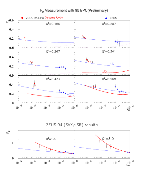
Figure 2: Preliminary ZEUS 1995 BPC $F_{2}$ measurements (top), together with ZEUS 1994 SVX/ISR data at higher $Q^{2}$ (bottom), from Ref. $\!{}^{{\bf?}}$. The predictions of the theoretical models from Refs. $\!{}^{{\bf?},{\bf?}}$ are also shown.

The kinematic range of the ZEUS data has been further extended by the installation in 1995 of a beam pipe calorimeter. This allows electron and positron scattering at smaller angles to be measured, which in turn leads, via Eq. (1), to smaller $Q^{2}$ values. Preliminary $F_{2}$ measurements, reported at the Workshop $\!{}^{{\bf?}}$, are shown in Fig. 2. The corresponding $x,Q^{2}$ range is

$$\mbox{ZEUS BPC}:\qquad 0.16\lower 3.01385pt\hbox{$\;\stackrel{{\scriptstyle\textstyle<}}{{\sim}}\;$}Q^{2}\lower 3.01385pt\hbox{$\;\stackrel{{\scriptstyle\textstyle<}}{{\sim}}\;$}0.57\;{\rm GeV}^{2},\qquad x\sim 10^{-5}\;.$$ (3)

Fig. 2 also illustrates the complementarity of the HERA and fixed-target structure function measurements. At the same low $Q^{2}$ values the E665 collaboration $\!{}^{{\bf?}}$ have measured $F_{2}^{\mu p}$ for $x\sim 10^{-3}-10^{-2}$, see Fig. 3. All these data are important for constraining models of structure functions at low $Q^{2}$. For example, the Donnachie-Landshoff Regge-based model $\!{}^{{\bf?}}$ appears to give a good description of the $Q^{2}\lower 3.01385pt\hbox{$\;\stackrel{{\scriptstyle\textstyle<}}{{\sim}}\;$}1\;{\rm GeV}^{2}$ data, interpolating between the ZEUS and E665 data with a slowly rising $F_{2}\sim x^{-0.08}$ form. However this model does not include pQCD $Q^{2}$ evolution, and therefore fails to describe the steepening of $F_{2}$ with increasing $Q^{2}$ which is apparent in the SVX/ISR data in Fig. 2. A comprehensive and critical review of models for $F_{2}$ at low $Q^{2}$ can be found in Ref. $\!{}^{{\bf?}}$

Figure 3: $F_{2}^{p}$ measurements by the E665 collaboration $\!{}^{{\bf?}}$, with various theoretical model predictions $\!{}^{{\bf?},{\bf?},{\bf?}}$.

Other new structure function data reported at the Workshop include updated measurements of $F_{2}^{p,d}$ and $F_{2}^{n}/F_{2}^{p}$ from the NMC collaboration $\!{}^{{\bf?}}$. These are particularly useful for constraining the medium-$x$ quark distributions (in particular the $u/d$ ratio) and will be incorporated in forthcoming ‘global fit’ analyses.

2.2 DGLAP evolution

One of the central tenets of perturbative QCD is that the $Q^{2}$ evolution of structure functions ${\cal F}_{i}(x,Q^{2})$ is determined by the DGLAP equations, provided that $Q^{2}$ is sufficiently large such that higher-twist ($\propto 1/Q^{2}$) contributions can be neglected. More precisely, the theory predicts the factorization scale dependence of the quark and gluon distributions, $q(x,\mu^{2})$ and $g(x,\mu^{2})$,

$$\mu^{2}{\partial\over\partial\mu^{2}}\;\left(\begin{array}[]{c}q\\ g\end{array}\right)\;=\;{\alpha_{s}(\mu^{2})\over 2\pi}\;\left(\begin{array}[]{cc}P_{qq}&P_{qg}\\ P_{gq}&P_{gg}\end{array}\right)\otimes\left(\begin{array}[]{c}q\\ g\end{array}\right)\;,$$ (4)

where $\otimes$ denotes a convolution integral and the splitting functions have a perturbative expansion

$$P_{ab}(x,\alpha_{s})=\alpha_{s}P_{ab}^{(0)}(x)+\alpha_{s}^{2}P_{ab}^{(1)}(x)+\ldots\;.$$ (5)

The structure functions are obtained as linear combinations of the parton distributions:

$${\cal F}_{i}(x,Q^{2}) = \int_{x}^{1}dy/y\left[\sum_{q}q(y,Q^{2})\otimes C_{q,i}(x/y,\alpha_{s}(Q^{2}))\right.$$ (6)

$$\left.+g(y,Q^{2})\otimes C_{g,i}(x/y,\alpha_{s}(Q^{2}))\right]\;.$$

For example, for ${\cal F}_{i}=x^{-1}F_{2}^{ep}$ the coefficient functions are $C_{q,i}(z,\alpha_{s})=e_{q}^{2}\delta(1-z)+O(\alpha_{s})$, $C_{g,i}(z,\alpha_{s})=O(\alpha_{s})$.

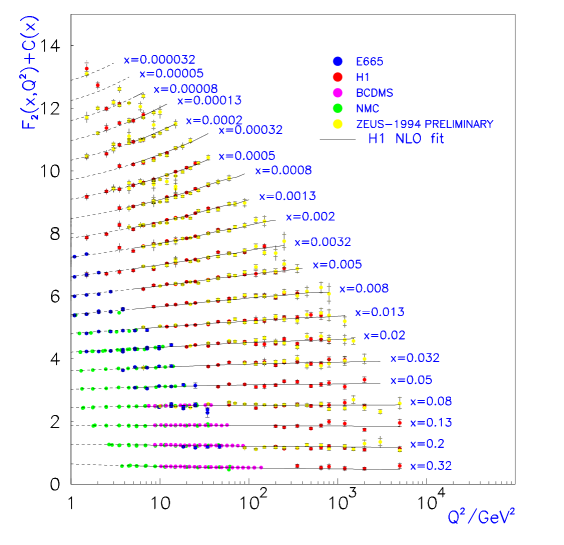
Figure 4: The $Q^{2}$ dependence of $F_{2}$ at small and medium $x$, together with a NLO QCD fit, from the H1 collaboration $\!{}^{{\bf?}}$.

Once the distributions $f_{i}(x,Q^{2})$ ($i=q,g$) and $\alpha_{s}$ are specified  at some ‘starting’ scale $Q_{0}^{2}$, the theory predicts the distributions at any $Q^{2}$ for which perturbation theory is valid. In practice the starting distributions are determined from the data by means of a global fit, see for example Refs. $\!{}^{{\bf?},{\bf?}}$. It is remarkable that only relatively simple functional forms are required, for example

$$xf_{i}(x,Q_{0}^{2})=A_{i}x^{-\lambda_{i}}(1+\epsilon_{i}\sqrt{x}+\gamma_{i}x)(1-x)^{\eta_{i}}\;.$$ (7)

The splitting and coefficient functions are known exactly at leading and next-to-leading order (see for example Ref. $\!{}^{{\bf?}}$ for a compilation and list of references). Truncating at this order defines the NLO DGLAP system of equations.

Several examples of NLO DGLAP fits to structure function data have been presented at the Workshop. Considering the wide range of processes and energies, the quality of the description is excellent. An example from the H1 collaboration $\!{}^{{\bf?}}$ is shown in Fig. 4. What information can be extracted from such fits? At large $x$ the DGLAP equation for $F_{2}$ reduces to $\partial F_{2}/\partial\ln Q^{2}\sim\alpha_{s}F_{2}\otimes P_{qq}$, and a precision measurement of $\alpha_{s}$ can be made, see Section 3 below. At small $x$ the gluon is the dominant parton and so $\partial F_{2}/\partial\ln Q^{2}\sim\alpha_{s}g\otimes P_{qg}$. Thus while $F_{2}$ directly measures the quark distribution at small $x$, its $Q^{2}$ variation measures the gluon.

The shape of the starting distributions (Eq. (7)) at small $x$ is determined by the parameters $\lambda_{i}$. The dominant partons here are the gluons and sea quarks, for which we may write

$$xg(x,Q_{0}^{2})\;\sim\;A_{g}x^{-\lambda_{g}}\;,\qquad xq_{S}(x,Q_{0}^{2})\;\sim\;A_{S}x^{-\lambda_{S}}\;.$$ (8)

It is interesting to see how $\lambda_{g}$ and $\lambda_{S}$, obtained from fits to data, have evolved with time. Table 1 shows these parameters for various recent MRS analyses. 

	set	$Q_{0}^{2}$	$\lambda_{S}$	$\lambda_{g}$
$<$1993		4	0	0
1993	D${}_{-}^{\prime}$	4	${\textstyle{1\over 2}}$	${\textstyle{1\over 2}}$
1994	A	4	0.3	0.3
1995	A′	4	0.17	0.17
1995	G	4	0.07	0.31
1996	R1	1	0.14	-0.41

Table 1: Evolution in time of the parameters determining the small-$x$ behaviour of the MRS quark and gluon distributions.

Before HERA data became available, it was traditional to assume Regge-motivated flat starting distributions ($\lambda\approx 0$). Subsequently, theoretical studies of the BFKL equation for resumming large logarithms of $1/x$ (see Section 2.4) suggested that the behaviour could in fact be much steeper ($\lambda\simeq 12\alpha_{s}\ln 2/\pi\approx 0.5$). The early HERA data showed a somewhat less steep rise at small $x$, with fits giving $\lambda\approx 0.3$. More recent HERA data show a preference for different $\lambda_{S}$ and $\lambda_{g}$ values. In fact in the most recent MRS fits $\!{}^{{\bf?}}$, where the minimum $Q^{2}$ of the fitted data is extended down to $1.5\;{\rm GeV}^{2}$, the gluon is ‘valence-like’ at the starting scale $Q_{0}^{2}=1\;{\rm GeV}^{2}$. Even more significant is the fact that the slope of the sea quark distribution is close to the Regge prediction obtained from fits to the energy dependence of total hadronic cross sections $\!{}^{{\bf?}}$:

$$xq_{S}\;\sim\;x^{1-\alpha_{\cal P}(0)\approx-0.08}\ \mbox{at}\ Q_{0}^{2}=O(1\;{\rm GeV}^{2})\;.$$ (9)

However the agreement between the fitted value of $\lambda_{S}$ and $\alpha_{\cal P}(0)-1$ should not be taken too literally. The former is an unphysical parameter, depending to some extent on the factorization scheme, the value chosen for $Q_{0}^{2}$, and the parametric form chosen for the starting distributions. Another problem with the Regge interpretation is that one would naively expect the gluon distribution to exhibit the same asymptotic behaviour for $x\to 0$. One can impose by hand the constraint $\lambda_{S}=\lambda_{g}$, in which case the common value $0.04$ (at $Q_{0}^{2}=1\;{\rm GeV}^{2}$) is obtained $\!{}^{{\bf?}}$, but the quality of the fit is worse than when the parameters are allowed to be different.

As Table 1 implies, the continual improvement in the structure function data requires a concomitant updating of the parton distributions derived from global fits. Thus ‘new’ data is able to discriminate between ‘old’ sets of partons. This is illustrated in Fig. 5, which shows recent HERA $F_{2}$ data compared with the 1995 MRS $\!{}^{{\bf?}}$ and 1994 GRV $\!{}^{{\bf?}}$ ‘dynamical parton’ predictions. Also shown is the new MRS(R₂) fit $\!{}^{{\bf?}}$ which includes these data. Notice how the MRS(G) and GRV(94) predictions are now disfavoured – they predict too strong a $Q^{2}$ dependence at small $x$. It will be interesting to see if the agreement between the dynamical parton model and the data can be restored by adjusting the parameters of the model, for example the value of the starting scale $\mu_{0}^{2}$ at which the distributions assume a valence-like form.

Figure 5: The description of the most recent HERA $F_{2}^{ep}$ data by the ‘old’ parton distributions of Refs. $\!{}^{{\bf?},{\bf?}}$, and the new MRS(R₂) fit $\!{}^{{\bf?}}$.

We can summarize the results of this section by the statement that the small-$x$ structure function data are consistent with DGLAP evolution starting from a soft input for both quarks and gluons at a scale of order $1\;{\rm GeV}^{2}$. The fact that the input is soft means that we can obtain a simple analytic approximation to the solutions of the evolution equation in the (double) asymptotic limit $Q^{2},\;1/x\to\infty$ $\!{}^{{\bf?}}$. In its simplest form, this result follows from the leading $x\to 0$ behaviour of the lowest-order splitting function matrix:

$$\mu^{2}{\partial\over\partial\mu^{2}}\;\left(\begin{array}[]{c}q\\ g\end{array}\right)\;\simeq\;{\alpha_{s}(\mu^{2})\over 2\pi}\;\left(\begin{array}[]{cc}0&0\\ {2C_{F}/x}&{2C_{A}/x}\end{array}\right)\otimes\left(\begin{array}[]{c}q\\ g\end{array}\right)\;,$$ (10)

which leads, for sufficiently soft starting distributions, to the prediction $\!{}^{{\bf?}}$

$$F_{2}\sim x\sum q\sim\exp\left[2\sqrt{{C_{A}\alpha_{s}\over\pi}\ln{Q^{2}\over Q_{0}^{2}}\ln{x_{0}\over x}}\right]\;.$$ (11)

Ball and Forte have extended this ‘double asymptotic scaling’ result to include subleading corrections and NLO contributions $\!{}^{{\bf?},{\bf?}}$. An example of a comparison between theory and experiment is shown in Fig. 6. Here $F_{2}$ has been rescaled by a factor which is essentially the right-hand side of (11), computed at NLO, in order to remove the leading asymptotic behaviour. The variables $\sigma,\rho$ are defined in terms of $x$ and $Q^{2}$ by

$$\sigma=\left[{\ln(x_{0}/x)\ln(t/t_{0})}\right]^{1/2}\;,\quad\rho=\left[{\ln(x_{0}/x)\over\ln(t/t_{0})}\right]^{1/2}\;,$$ (12)

where $t=\ln(Q^{2}/\Lambda^{2})$. The fact that the data lie approximately on universal, horizontal bands is a demonstration of the validity of double asymptotic scaling. A slight breaking of the scaling behaviour is evident at large and small $\rho$ in the lower plot, where, respectively, $Q^{2}$ becomes too small and $x$ becomes too large for the approximation to be valid. Here, however, the full NLO DGLAP prediction (indicated by the curves) gives a very good description.

Figure 6: H1 $F_{2}$ data compared with the ‘double asymptotic scaling’ prediction $\!{}^{{\bf?}}$. The curves are the full NLO best fit and have $\rho=2,3,4$ in the $\sigma$ plot, and $\sigma=1,1.2,1.4$ in the $\rho$ plot.

2.3 Beyond NLO DGLAP at small $x$

Why does NLO DGLAP evolution work so well? To attempt to answer this, we consider two types of correction which could in principle be important in particular regions of $x,Q^{2}$ space. First, we note that the statement that ‘perturbative QCD evolution describes the data down to $Q^{2}\sim 1\;{\rm GeV}^{2}$’ must be qualified by the condition ‘at small $x$’. At large $x$ it has been clearly shown that higher-twist (i.e. $1/Q^{2}$) contributions to the structure functions are important. In Ref. $\!{}^{{\bf?}}$, a combined leading-twist/higher-twist analysis of structure function data, using the empirical form

$$F_{2}^{(HT)}(x,Q^{2})=F_{2}^{(LT)}(x,Q^{2})\ {C(x)\over Q^{2}}\;,$$ (13)

gave $C\approx 0.3\;{\rm GeV}^{2}/(1-x)$ at large $x$ and $C\approx 0$ at small $x$. The factor $(1-x)^{-1}$ is not unexpected, since there are $j$ times more operators which contribute to the $j$th moment of $F_{2}^{(HT)}$ than to $F_{2}^{(LT)}$. Therefore at large $j$ the moments are expected to differ by a factor of $j$, corresponding to a factor $(1-x)^{-1}$ difference in the contributions to the structure function. Although the analysis of Ref. $\!{}^{{\bf?}}$ was restricted to fixed-target data with $x\lower 3.01385pt\hbox{$\;\stackrel{{\scriptstyle\textstyle>}}{{\sim}}\;$}0.1$ it would appear that the small-$x$ HERA structure functions with $Q^{2}\lower 3.01385pt\hbox{$\;\stackrel{{\scriptstyle\textstyle>}}{{\sim}}\;$}1.5\;{\rm GeV}^{2}$ are also relatively free from higher-twist contributions. In fact a global fit to the HERA ($Q^{2}>1.5\;{\rm GeV}^{2}$) $F_{2}$ data which includes a phenomenological higher-twist contribution of the form $(a^{2}/Q^{2})F_{2}^{(LT)}$ gives a value for $a^{2}$ consistent with zero $\!{}^{{\bf?}}$.

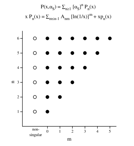
Figure 7: Pattern of $\ln(1/x)$ coefficients in the splitting functions at small $x$.

A second important correction to NLO DLGAP evolution at small $x$ comes from higher-order terms on the right-hand side of (5). As $x\to 0$, large $L_{x}\equiv\ln(1/x)$ logarithms appear in the splitting functions and spoil the convergence. The theory and phenomenology of these logarithms have been extensively discussed at this Workshop $\!{}^{{\bf?}}$. In general one can show that there are at most $n-1$ large logarithms in the $n$th order splitting function, i.e.

$$xP^{(n)}(x)=A_{n,n-1}L_{x}^{n-1}+A_{n,n-2}L_{x}^{n-2}+\ldots+A_{n,0}+xp^{(n)}(x)\;,$$ (14)

where $p^{(n)}$ is finite in the limit $x\to 0$. The full splitting function is then

$$xP(x,\alpha_{s})=\sum_{n=1}^{\infty}\left({\alpha_{s}\over 2\pi}\right)^{n}\left[\sum_{m=0}^{n-1}A_{n,m}L_{x}^{m}+xp^{(n)}(x)\right]\;.$$ (15)

This expression holds for all four splitting functions, $P_{gg}$, $P_{qg}$, $P_{gq}$ and $P_{qq}$. The pattern of the coefficients is illustrated in Fig. 7. The horizontal rows represent the complete splitting function at a given order in perturbation theory, for example LO$(n=1$), NLO$(n=2)$, etc. The leading diagonal with $n=m+1$ represents the set of leading $L_{x}$ contributions, and so on.

Of particular phenomenological importance is the $P_{qg}$ function, since at small $x$ $\partial F_{2}/\partial\ln Q^{2}\sim\alpha_{s}P^{qg}\otimes g$. To illustrate the importance of the higher-order contributions, it is convenient to take moments, $\gamma(\omega)=\int_{0}^{1}dx\;x^{\omega}\;P(x)$, so that $xP(x)\sim L_{x}^{n-1}\Rightarrow\gamma(\omega)\sim\Gamma(n)/\omega^{n}$. The leading behaviour as $\omega\to 0$ (equivalently $x\to 0$) of $\gamma^{qg}$ is found to be $\!{}^{{\bf?}}$ (with $\bar{\alpha}_{s}=3\alpha_{s}/\pi$)

$$\gamma^{qg}(\omega)=n_{f}{\bar{\alpha}_{s}\over 9}\left[\left(1+\ldots\right)+\bar{\alpha}_{s}\left({2.17\over\omega}+\ldots\right)+\bar{\alpha}_{s}^{2}\left({2.30\over\omega^{2}}+\ldots\right)+\ldots\right]\;,$$ (16)

where at each order in perturbation theory subleading terms down by one or more powers of $\omega$ have been suppressed. In fact beyond NLO only the leading $\bar{\alpha}_{s}(\bar{\alpha}_{s}/\omega)^{n}$ coefficients are known. In the limit $\bar{\alpha}_{s}L_{x}\gg 1$ they resum to give the characteristic BFKL ‘perturbative pomeron’ behaviour $\!{}^{{\bf?}}$

$$xP_{qg}\sim x^{-4\ln 2\;\bar{\alpha}_{s}}\;.$$ (17)

This asymptotic limit is, however, not relevant for the HERA structure function data. The interesting question is how important in practice are the contributions beyond NLO in (16). Certainly the leading logarithm part of these contributions appears to be large. This is illustrated in Fig. 8, which compares the exact leading- and next-to-leading-order contributions with the leading-logarithm part of the first five orders in perturbation theory.

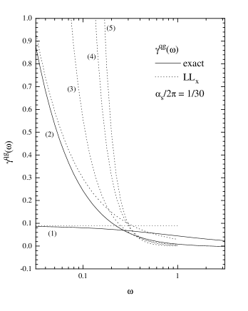
Figure 8: The anomalous dimension $\gamma^{qg}(\omega)$, showing the exact first- and second-order contributions, together with the leading-logarithm parts of the first five orders.

It would appear from Fig. 8 that the higher-order terms could be phenomenologically important. On the other hand, retaining only the leading terms at each order (as in the phenomenological analyses performed so far) could well overestimate their importance. This is evidently true of the LO and NLO contributions in the region $0.1\lower 3.01385pt\hbox{$\;\stackrel{{\scriptstyle\textstyle<}}{{\sim}}\;$}\omega\lower 3.01385pt\hbox{$\;\stackrel{{\scriptstyle\textstyle<}}{{\sim}}\;$}1$. Certainly, there is no evidence that the data require such contributions. One can quantify this statement $\!{}^{{\bf?}}$ by replacing $\ln(1/x)$ in the leading-logarithm expansion by $\ln(x_{0}/x)\theta(x_{0}-x)$, and regarding $x_{0}$ as a parameter to be determined by the data. Note that this replacement has the effect of artificially introducing sub-leading logarithms, since $L_{x}^{n}\to L_{x}^{n}+n\ln(x_{0})L_{x}^{n-1}+\ldots\;$. Fig. 9 shows the $\chi^{2}$ of the fit to the HERA $F_{2}$ data as a function of $x_{0}$ (in various resummation schemes, see $\!{}^{{\bf?},{\bf?}}$).

Figure 9: $\chi^{2}$ of various resummed $\ln(1/x)$ fits to the HERA $F_{2}$ data versus $x_{0}$, from Ref. $\!{}^{{\bf?}}$.

In each scheme the minimum value of $\chi^{2}$ is attained for $x_{0}\to 0$, indicating that the data prefer fits without the higher-order leading $\ln(1/x)$ contributions.

2.4 ‘BFKL’ description of $F_{2}$

In the double asymptotic limit discussed in Section 2.2, the evolution equation sums leading powers of $[\alpha_{s}\ln(1/x)\ln Q^{2}]^{n}$ generated by multigluon emission, and the distributions increase faster than any power of $\ln(1/x)$ as $x\rightarrow 0$, see (11). The dominant region of phase space is where the gluons have strongly-ordered transverse momenta, $Q^{2}\gg k^{2}_{Tn}\gg...\gg k^{2}_{T1}$. However such evolution does not include all the leading terms in the small-$x$ limit. It neglects those terms which contain the leading power of $\ln(1/x)$ but which are not accompanied by the leading power of $\ln Q^{2}$. The BFKL equation $\!{}^{{\bf?}}$, on the other hand, sums the leading $\ln(1/x)$ terms while retaining the full $Q^{2}$ dependence. The integration is taken over the full $k_{T}$ phase space of the gluons, not just the strongly-ordered part. The result is most conveniently established for the gluon distribution unintegrated over $k_{T}$,

$$xg(x,Q^{2})=\int^{Q^{2}}dk_{T}^{2}\;{\cal G}(x,k_{T}^{2}),$$ (18)

and is

$${\cal G}(x,k_{T}^{2})\;\;\sim\;\;h(k_{T}^{2})x^{-\lambda},$$ (19)

where $h\sim(k_{T}^{2})^{-1/2}$ at large $k_{T}^{2}$ and $\lambda$ is the the maximum eigenvalue of the kernel $K$ of the BFKL equation

$${\partial{\cal G}\over\partial L_{x}}=\int d^{2}k_{T}^{\prime}\;K(\vec{k}_{T},\vec{k}_{T}^{\prime})\;{\cal G}(x,k_{T}^{\prime 2})\;.$$ (20)

For fixed $\alpha_{s}$, $\lambda=12\ln 2\alpha_{s}/\pi\approx 0.5$. The prediction for $F_{2}$ is obtained by using the $k_{T}$-factorization theorem $\!{}^{{\bf?}}$

$$F_{2}(x,Q^{2})=\int_{x}^{1}{dx^{\prime}\over x^{\prime}}\int{dk_{T}^{2}\over k_{T}^{4}}{\cal G}\left({x\over x^{\prime}},k_{T}^{2}\right)\overline{F}_{2}(x^{\prime},k_{T}^{2},Q^{2}),$$ (21)

where $\overline{F}_{2}$ denotes the quark-box contribution $\gamma g\to q\bar{q}$ for the scattering of a photon of virtuality $Q^{2}$ off a gluon with longitudinal momentum fraction $x^{\prime}$ and transverse momentum $k_{T}$.

Figure 10: Constrained CCFM description of $F_{2}$ at small $x$ $\!{}^{{\bf?}}$.

In recent years there have been several numerical analyses of the solution of the BFKL equation and of the corresponding predictions for $F_{2}$, based on the above results (for a review see $\!{}^{{\bf?}}$). The ‘naive’ BFKL prediction,

$$F_{2}(x,Q^{2})=C(Q^{2})x^{-\lambda}+F_{2}^{\rm NP},$$ (22)

where $\lambda\approx 0.5$ and $F_{2}^{\rm NP}$ is a non-perturbative background contribution which is constant at small $x$, would appear to give too steep a rise in $x$. However there has been significant recent progress, reported at this Workshop $\!{}^{{\bf?}}$, towards a ‘unified’ treatment which incorporates both DGLAP and BFKL dynamics, embodied in the so-called CCFM equation, together with appropriate kinematic constraints. A reasonable description of the HERA data is obtained $\!{}^{{\bf?}}$, see Fig. 10. Here the continuous curves are the CCFM predictions with and without the kinematic constraints. From a theoretical point of view, the attraction of the BFKL approach is that it attempts to explain the shape of the small-$x$ structure function from first principles. However, at present one cannot discriminate between the DGLAP and BFKL predictions on the basis of the $x$ and $Q^{2}$ dependence of $F_{2}$ alone. Furthermore, it is not clear how much truly ‘BFKL’ dynamics remains in the kinematically-constrained CCFM equation applied to the HERA kinematic region. A key test would appear to be provided by more exclusive quantities, such as the average transverse hadronic energy in deep inelastic events (which is predicted to be larger in the BFKL approach) and the cross section for producing forward, moderate $E_{T}$ jets $\!{}^{{\bf?}}$.

2.5 Gluon determinations

Deep inelastic structure functions directly measure the quark distribution functions. The precision is set by the experimental measurements, and is at the level of a few percent over a wide range in $x$, at least for the $u$ and $d$ quarks. The gluon is much less well determined: a variety of hard scattering processes provide measurements in particular $x$ regions at different $Q^{2}$ scales, and momentum conversation pins down the first moment to a few percent.

Several new results on the gluon determination have been reported at this Workshop. An overview is given in Ref. $\!{}^{{\bf?}}$. We will concentrate here on those new results which are ‘theoretically precise’, i.e. are performed using cross sections calculated to next-to-leading order. This allows the gluon to be defined and extracted according to a particular factorization scheme (e.g. $\overline{\mbox{MS}}$), as for the quark distributions.

For $x\lower 3.01385pt\hbox{$\;\stackrel{{\scriptstyle\textstyle<}}{{\sim}}\;$}0.01$, the $Q^{2}$ dependence of $F_{2}$ is dominated by the gluon contribution to the right-hand side of the evolution equation,

$$\frac{\partial F_{2}(x,Q^{2})}{\partial\ln Q^{2}}\simeq\frac{\alpha_{s}(Q^{2})}{\pi}\sum_{q}e^{2}_{q}\;\int^{1}_{x}\frac{dy}{y}\left(\frac{x}{y}\right)P_{qg}\left(\frac{x}{y}\right)yg(y,Q^{2})\;.$$ (23)

The uncertainty in the gluon obtained from the HERA data in this way has steadily decreased in the last few years. As an example, Fig. 11 shows the gluon obtained from the H1 NLO QCD fit $\!{}^{{\bf?}}$.

Figure 11: The gluon distribution obtained by H1 from a global NLO QCD fit $\!{}^{{\bf?}}$.

The shaded band represents the combined systematic and statistical error – approximately $\pm 20\%$ over the range in $x$ ($10^{-4}-10^{-2}$) where there is sensitivity. It is interesting to compare the gluon of Fig. 11 with that obtained from a global fit. Fig. 12 shows the gluons at $5\;{\rm GeV}^{2}$ from the latest MRS(R) series of fits $\!{}^{{\bf?}}$, together with several ‘old’ gluons.

Figure 12: Gluon distributions at $Q^{2}=5\;{\rm GeV}^{2}$ from the latest MRS(R) fits $\!{}^{{\bf?}}$.

At small $x$ ($\sim 10^{-4}$) there is good agreement with the H1 gluon, and the spread of the new MRS gluons is similar to the uncertainty band in Fig. 11. However for $x\lower 3.01385pt\hbox{$\;\stackrel{{\scriptstyle\textstyle>}}{{\sim}}\;$}10^{-2}$ the MRS gluon distributions are systematically smaller than the H1 gluon. This is due to the extra constraints (principally from momentum conservation and from prompt photon production) imposed in the global fit.

There has been considerable discussion at this Workshop about the new large $E_{T}$ jet data from CDF and D0 $\!{}^{{\bf?}}$. It is not yet clear whether the apparent excess of data over theory seen in the CDF data for $E_{T}\lower 3.01385pt\hbox{$\;\stackrel{{\scriptstyle\textstyle>}}{{\sim}}\;$}200\;{\rm GeV}$ is a real effect, and if so whether it is due to harder parton distributions than previously estimated $\!{}^{{\bf?},{\bf?}}$ or to some ‘new physics’ contribution. What is clear is that the jet data for $E_{T}\lower 3.01385pt\hbox{$\;\stackrel{{\scriptstyle\textstyle<}}{{\sim}}\;$}200\;{\rm GeV}$ have considerable potential for constraining the gluon distribution ($qg\to qg$ is the dominant subprocess) and $\alpha_{s}$. The CTEQ collaboration have already incorporated the CDF jet data into their global fits $\!{}^{{\bf?}}$. As an example, Fig. 13 shows a series of CTEQ gluon distributions obtained assuming different $\alpha_{s}(M_{Z}^{2})$ values in the range $[0.105,0.122]$. The effect of the jet data is seen in the difference between the new gluons and the CTEQ(3M) gluon in the $x\sim 0.1-0.3$ range. Notice also the correlation with the $\alpha_{s}$ value. From such analyses, one may conclude that the uncertainty in the gluon  has now been reduced to $O(\pm 10\%)$ over a broad range in $x$, rising to $O(\pm 20\%)$ at small $x\sim 10^{-4}$. This represents considerable progress!

Figure 13: New CTEQ gluon distributions at $5\;{\rm GeV}^{2}$ from fits incorporating CDF jet data$\!{}^{{\bf?}}$.

The gluon distribution can also be determined at HERA from the ‘$2+1$’ jet cross section, i.e. the cross section for producing an additional hard hadronic jet in addition to the current and beam remnant jets. Preliminary results had already been reported in Paris last year, but what is new this year is that the analysis can now be done consistently to next-to-leading order in perturbation theory. The key here is the recent availability of NLO QCD Monte Carlo programs such as PROJET $\!{}^{{\bf?}}$ and MEPJET $\!{}^{{\bf?}}$. At leading order the cross section is, schematically,

$$\sigma(2+1)=\sum_{q}\left[q\otimes\hat{\sigma}(\gamma^{*}q\to qg)\;+\;g\otimes\hat{\sigma}(\gamma^{*}g\to q\bar{q})\right]\;.$$ (24)

Note that the subprocess cross sections are $O(\alpha_{s})$, and in fact this allows a reasonably precise determination of the strong coupling, see Section 3. The parton distributions in (24) are probed at $x=x_{\rm Bj}(1+M^{2}_{jj}/Q^{2})$, where $M^{2}_{jj}$ is the invariant mass of the final-state jet pair. In practice, the range covered at HERA is approximately $0.01\lower 3.01385pt\hbox{$\;\stackrel{{\scriptstyle\textstyle<}}{{\sim}}\;$}x\lower 3.01385pt\hbox{$\;\stackrel{{\scriptstyle\textstyle<}}{{\sim}}\;$}0.1$. The importance of this is that it ‘fills in’ the gap between the small-$x$ scaling violation and large-$x$ prompt photon methods for determining the gluon. Both the H1 $\!{}^{{\bf?}}$ and ZEUS $\!{}^{{\bf?}}$ collaborations have reported new results on the gluon distribution from $\sigma(2+1)$ at this Workshop. Fig. 14 shows the gluon distribution at $20\;{\rm GeV}^{2}$ extracted by H1. The band corresponds to the combined systematic and statistical error. Note that there is good agreement with the standard gluons obtained from global fits. With a further reduction in the statistical and systematic errors, this method of determining the gluon will play an important role in the overall constraint picture.

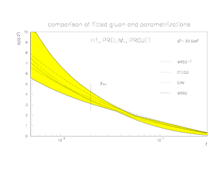
Figure 14: H1 $2+1$ jet gluon distribution $\!{}^{{\bf?}}$.

Finally, we should mention also a new method of determining the gluon distribution from diffractive ${\rm J}/\psi$ electro- (and photo-) production: ${\rm e}+{\rm p}\to{\rm e}+{\rm J}/\psi+{\rm p}$. For sufficiently high $W^{2}$ the scattering amplitude can be calculated perturbatively $\!{}^{{\bf?}}$, reducing (at lowest order) to the scattering of the $c\bar{c}$ system off the proton via two gluon colour-singlet exchange. The lowest-order result is

$${d\sigma\over dt}(\gamma^{*}p\to J/\psi p)={\Gamma_{ee}M_{\psi}^{2}\pi^{3}\alpha_{s}(\overline{Q}^{2})^{2}\over 48\alpha\overline{Q}^{6}}\;\left[\bar{x}g(\bar{x},\overline{Q}^{2})\right]^{2}\;\left(1+{Q^{2}\over M_{\psi}^{2}}\right)\;,$$ (25)

where

$$\overline{Q}=(Q^{2}+M_{\psi}^{2})/4\;,\qquad\bar{x}=4\overline{Q}^{2}/W^{2}\;.$$ (26)

At higher orders, and when $\bar{x}$ is small, two gluon exchange is replaced by a generalized ‘BFKL’ gluon ladder, i.e. the unintegrated gluon distribution ${\cal G}(x,k_{T}^{2})$ discussed in Section 2.4, but the basic structure remains the same $\!{}^{{\bf?}}$. Phenomenological studies based on the above theoretical approach have recently been performed $\!{}^{{\bf?},{\bf?}}$. The $W^{2}$ dependence of the cross section is a direct measure of the shape of the gluon distribution, and the sensitivity is enhanced by the fact that it enters squared in the expression for the cross section. Fig. 15 $\!{}^{{\bf?}}$ compares the predictions based on various gluon distributions with recent fixed-target and HERA data. Note that the theoretical calculations do not yet include the complete $O(\alpha_{s})$ corrections to the cross sections, and cannot therefore distinguish gluons corresponding to different factorization schemes. In view of the potential of this method for constraining the gluon at small $x$, the calculation of the NLO corrections would be very worthwhile.

Figure 15: Diffractive $J/\psi$ photoproduction cross section data compared with theoretical predictions based on various gluon distributions $\!{}^{{\bf?}}$.

2.6 High $Q^{2}$

Over most of the measured $Q^{2}$ range in Fig. 1, the deep inelastic cross section is dominated by the neutral current contribution, Fig. 16(a).

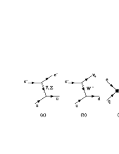
Figure 16: (a) Neutral current, (b) charged current and (c) contact interaction contributions to electron–quark scattering at high $Q^{2}$.

With increased statistics at high $Q^{2}$ ($\lower 3.01385pt\hbox{$\;\stackrel{{\scriptstyle\textstyle>}}{{\sim}}\;$}10^{4}\;{\rm GeV}^{2}$), HERA can also measure the structure of the proton as seen by the charged weak current, Fig. 16(b). The corresponding deep inelastic cross section is

$${d^{2}\sigma^{CC}\over dxdQ^{2}}={(1-\lambda_{e})\pi\alpha^{2}\over 8\sin^{4}\theta_{W}(Q^{2}+M_{W}^{2})^{2}}\sum_{i,j}\left[|V_{u_{i}d_{j}}|^{2}u_{i}(x)+(1-y)^{2}|V_{u_{j}d_{i}}|^{2}d_{i}(x)\right],$$ (27)

where $\lambda_{e}$ is the helicity of the electron, $u_{i}$ and $d_{i}$ refer to up- and down-type quarks respectively, and the $V_{u_{i}d_{j}}$ are the elements of the CKM matrix. In principle this allows a different combination of parton distributions to be measured. Some preliminary results have been reported at this Workshop $\!{}^{{\bf?}}$. The data clearly show the convergence of the charged and neutral current cross sections at very high $Q^{2}$, $d\sigma^{CC}/dxdQ^{2}\sim d\sigma^{NC}/dxdQ^{2}\sim Q^{-4}$, see Fig. 17. The fact that the high-$Q^{2}$ cross sections agree with the DGLAP–based extrapolations enables limits to be placed on possible contact interactions, as expected on general grounds in composite models.

Figure 17: Charged and neutral current deep inelastic cross sections from H1 at HERA $\!{}^{{\bf?}}$.

The convention (see for example $\!{}^{{\bf?}}$) is to parametrize such interactions using the Lagrangian

$$\Delta{\cal L}={4\pi\eta\over\Lambda^{2}}\;\sum_{q,l}({\bar{q}}\gamma^{\mu}q)_{L,R}\;({\bar{l}}\gamma_{\mu}l)_{L,R}\;,$$ (28)

which leads to additional contributions to the cross section of order $Q^{-2}\Lambda^{-2}$ and $\Lambda^{-4}$. The parameter $\Lambda$ is a measure of the compositeness scale, and $\eta$ determines whether the interference with the Standard Model cross section is constructive or destructive. An example of how the data can be used to constrain $\Lambda$ is shown in Fig. 18 from ZEUS $\!{}^{{\bf?}}$. Here a particular (left–right) helicity structure has been assumed for the lepton–quark contact interaction.

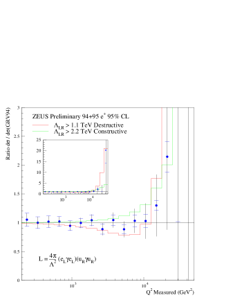
Figure 18: Limits on lepton–quark contact interactions from high-$Q^{2}$ neutral current DIS data, from ZEUS $\!{}^{{\bf?}}$.

The actual lower limits on $\Lambda$ depend slightly on this structure, and are typically $O(1\;{\rm TeV})$ and $O(2\;{\rm TeV})$ for destructive and constructive interference respectively. Note that somewhat higher limits ($3-4\;{\rm TeV}$) are obtained from Drell-Yan ($q\bar{q}\to l^{+}l^{-}$) lepton-pair production at the Fermilab Tevatron collider $\!{}^{{\bf?}}$.

3 $\alpha_{s}$ measurements

Deep inelastic scattering has traditionally provided some of the most precise measurements of the strong coupling $\alpha_{s}$. There are three basic methods:

• scaling violations of structure functions,

• structure function sum rules,

• jet cross sections.

Some of the high-precision values  obtained using these methods are listed in Table 2.

measurement	experiment	$\langle Q\rangle$	pQCD	$\alpha_{s}^{\overline{\rm MS}}(M_{Z}^{2})$
$\partial F_{2}^{lN}/\partial\ln Q^{2}$	SLAC/BCDMS $\!{}^{{\bf?}}$	$7.1$	NLO	$0.113\pm 0.005$
$\partial F_{2}^{\nu N}/\partial\ln Q^{2}$	CCFR $\!{}^{{\bf?}}$	$5.0$	NLO	$0.111\pm 0.006$
$\int_{0}^{1}dx(F_{3}^{\nu N}+F_{3}^{\bar{\nu}N})$	CCFR $\!{}^{{\bf?}}$	$1.73$	NNLO	$0.108^{+0.006}_{-0.009}$
$\int_{0}^{1}dx(g_{1}^{p}-g_{1}^{n})$	SLAC/EMC/SMC $\!{}^{{\bf?}}$	$1.58$	NNLO	$0.122^{+0.005}_{-0.009}$
$\sigma^{\gamma^{*}p}(2+1\;\mbox{jet})$	H1, ZEUS $\!{}^{{\bf?}}$	$22.1$	NLO	$0.118\pm 0.009$

Table 2: Some deep inelastic scattering $\alpha_{s}$ measurements.

The errors are between 5% and 10%, with the highest accuracy coming from the scale variation of the structure functions. More importantly, all the results agree within errors. These ‘deep inelastic’ $\alpha_{s}$ measurements also have a significant weight in the overall world average value, which is currently $\!{}^{{\bf?}}$

$$\alpha_{s}(M_{Z}^{2})=0.116\pm 0.005\;.$$ (29)

The value of $\alpha_{s}$ obtained from scaling violations has been discussed widely at this Workshop, especially in connection with new information coming from the HERA $F_{2}$ data. It is important to recall that the ‘gold-plated’ values in Table 2 come from the high-precision fixed-target data. In particular, in the analysis of Ref. $\!{}^{{\bf?}}$, which includes lower energy SLAC data and a phenomenological contribution from higher-twists, the resolving power on $\alpha_{s}$ comes from data with $0.3\lower 3.01385pt\hbox{$\;\stackrel{{\scriptstyle\textstyle<}}{{\sim}}\;$}x\lower 3.01385pt\hbox{$\;\stackrel{{\scriptstyle\textstyle<}}{{\sim}}\;$}0.5$ (see Fig. 19) and $10\lower 3.01385pt\hbox{$\;\stackrel{{\scriptstyle\textstyle<}}{{\sim}}\;$}Q^{2}\lower 3.01385pt\hbox{$\;\stackrel{{\scriptstyle\textstyle<}}{{\sim}}\;$}100\;{\rm GeV}^{2}$. In this kinematic region, higher-order perturbative and higher-twist corrections should be very small.

Figure 19: Logarithmic $Q^{2}$ derivative of the $F_{2}$ structure function measured off hydrogen and deuterium targets compared to NLO predictions, from Ref. $\!{}^{{\bf?}}$.

In the last year it has become clear that the HERA structure function data prefer a slightly larger $\alpha_{s}$ value than the fixed-target data at higher $x$, a result first pointed out in Ref. $\!{}^{{\bf?}}$. For example, in the NLO analysis of the 1993 data reported in Ref. $\!{}^{{\bf?}}$, the value $\alpha_{s}(M_{Z}^{2})=0.120\pm 0.005({\rm exp.})\pm 0.009({\rm th.})$ was obtained (for an update see Ref. $\!{}^{{\bf?}}$), with the theory error dominated by the variation with respect to the renormalization and factorization scale. In the new MRS analysis $\!{}^{{\bf?}}$, which includes the new 1994 HERA data, fits are performed with two $\alpha_{s}$ values, $0.113$ and $0.120$. The latter value is motivated by (a) the preference of the LEP/SLC three-jet and total $Z$ hadronic width data for a larger $\alpha_{s}$ value (see for example Ref. $\!{}^{{\bf?}}$), and (b) the fact that the Fermilab inclusive medium–$E_{T}$ jet data is slightly steeper than the theoretical prediction using partons with $\alpha_{s}\simeq 0.113$ $\!{}^{{\bf?},{\bf?}}$. Table 3 shows the $\chi^{2}$ values for the MRS fits $\!{}^{{\bf?}}$ to the H1 and ZEUS data with the two different $\alpha_{s}$ values. Both experiments show a clear preference for the larger value.

expt.	$\chi^{2}({\rm R}_{1})$	$\chi^{2}({\rm R}_{2})$
	$\alpha_{s}=0.113$	$\alpha_{s}=0.120$
H1 (193 pts)	182	168
ZEUS (210 pts)	391	362

Table 3: $\chi^{2}$ values for the new MRS(R₁,R₂) fits to the HERA $F_{2}$ data $\!{}^{{\bf?}}$.

What could be responsible for this apparent difference in the small- and large-$x$ $\alpha_{s}$ values (if one ignores the fact that within the overall errors there is no significant disagreement!)? So far there has been no proper study of the dependence of the $\alpha_{s}$ value on the way the charm contribution to $F_{2}$ is treated. This is almost certainly insignificant at large $x$, but could make a slight difference at small $x$ where the charm contribution is expected to be a more significant fraction of the total structure function, and where the threshold $Q^{2}$ dependence of $F_{2}^{c}$ could perhaps ‘fake’ a stronger DGLAP $Q^{2}$ variation. Second, we have already seen that higher-order contributions to DGLAP evolution become more and more important as $x\to 0$. It could well be that the larger $\alpha_{s}$ value at small $x$ is an indication that the (as yet unknown) NNLO corrections are not negligible. A complete calculation of the third-order splitting functions would almost certainly settle this issue.

New analyses of $\alpha_{s}$ from the deep inelastic $2+1$ jet cross section (Eq. (24)) by H1 and ZEUS have also been reported at this Workshop $\!{}^{{\bf?},{\bf?}}$. It appears that there may have been a slight problem with the previous analyses $\!{}^{{\bf?}}$ arising from a mismatch of the jet algorithm used in the NLO theoretical calculation and that employed in the experimental analyses. In general, jets are defined using a cluster algorithm which is applied to hadrons and partons in the experimental and theoretical analyses respectively. One defines a dimensionless ‘metric’ between two hadrons (say), $y_{ij}=s_{ij}/M^{2}$, and merges the hadrons into a single cluster if $y_{ij}<y_{\rm cut}$, where $y_{\rm cut}$ is a fixed (small) number. Various choices for $s_{ij}$ ($=2E_{i}E_{j}(1-\cos\theta_{ij})$ [JADE], $={\rm min}\,k_{Tij}^{2}$ [Durham/$k_{T}$], …) and $M^{2}$ ($=Q^{2},W^{2},\ldots$) are possible, but in each case the theoretical calculation must be matched to the experimental definition – the NLO corrections are in general different for the different jet definitions. The new MEPJET theory Monte Carlo $\!{}^{{\bf?}}$ allows an arbitrary algorithm to be used, and can therefore be tuned to the experimental analysis. Although there are still some questions to be answered (the effect of hadronization, the correlation of $\alpha_{s}$ with the gluon distribution, the sensitivity to the jet cuts, etc.), it is already clear that this is a potentially powerful method for measuring the strong coupling at HERA in the future. It will be very interesting to see if the value thus obtained agrees with the scaling violation value. 

4 Spin physics

Polarized deep inelastic scattering experiments provide information about how the spin of the hadron is shared among its parton constituents. As for unpolarized scattering, the cross section can be related to two structure functions, $g_{1}$ and $g_{2}$. The former is analogous to $F_{1}$, and in the parton model is given by a sum over polarized quark distribution functions:

$$g_{1}(x)={\textstyle{1\over 2}}\sum_{q}e_{q}^{2}[\Delta q(x)+\Delta\bar{q}(x)]\;.$$ (30)

with $\Delta q=q^{\uparrow}-q^{\downarrow}$. In perturbative QCD, the distributions $\Delta q$ and $\Delta g$ acquire a scale dependence given by the polarized versions of the DGLAP equations ($\Delta$DGLAP). The first moments, $\int_{0}^{1}dx\Delta q_{i}$ and $\int_{0}^{1}dx\Delta g$, represent the net spin carried by the various partons. The former can be related to axial-vector couplings measured in hyperon decay. In addition, the Bjorken sum rule ($\int_{0}^{1}dx(g_{1}^{p}-g_{1}^{n})={1\over 6}|{g_{A}/g_{V}}|[1+O(\alpha_{s})]$) provides a fundamental test of the theory.

There are currently several important theoretical issues:

• How much of the spin is carried by each type of parton; in particular, how much is carried by strange quarks and gluons?

• Is the observed $Q^{2}$ dependence of the structure functions consistent with $\Delta$DGLAP evolution?

• How large is $g_{2}$ and is it consistent with model calculations?

• Can the theory predict the $x\to 0$ behaviour of the polarized distributions, as for unpolarized distributions (see Section 2.4)?

Answers to all of these questions require precision input from experiments. The last few years have seen a rapid growth in the amount of data available. At this Workshop, the SMC collaboration $\!{}^{{\bf?}}$ have reported new measurements of $g_{1}^{d}$, $g_{2}$ and the semi-inclusive process $\mu N\to NhX$. The SLAC E-143 collaboration $\!{}^{{\bf?}}$ have reported new measurements of $g_{2}$ and the $Q^{2}$ dependence of $g_{1}^{p,d}$. But perhaps the most significant development has been the first results from the HERMES experiment at DESY $\!{}^{{\bf?}}$. Fig. 20 shows preliminary results on $g_{1}^{n}$. The results are in agreement with published SLAC-E142 measurements $\!{}^{{\bf?}}$ which cover approximately the same kinematic range. One of the advantages of the HERMES experiment is the ability to measure semi-inclusive processes, i.e. $e^{\uparrow\downarrow}p^{\uparrow\downarrow}\to e+h+X$. The cross section for this is, schematically,

$$\Delta\sigma^{h}(x,z)\sim\sum_{q}\Delta q(x)D_{\Delta q\to h}(z)\;.$$ (31)

The identification of the charge and flavour of hadrons in the final state therefore gives a more powerful handle on the various $\Delta q$, in particular the separation between valence and sea quarks. Quantitative results from HERMES are expected soon.

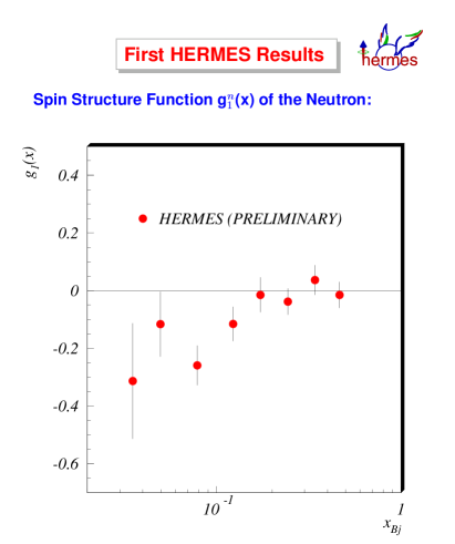
Figure 20: The spin structure function $g_{1}^{n}(x)$ from HERMES $\!{}^{{\bf?}}$.

New theoretical developments have also been reported at this Workshop. The major advance in the last year has been the calculation of the two-loop ($O(\alpha_{s}^{2})$) polarized splitting functions $\!{}^{{\bf?}}$,

$$\Delta P_{ab}(x,\alpha_{s})=\alpha_{s}\Delta P_{ab}^{(0)}(x)+\alpha_{s}^{2}\Delta P_{ab}^{(1)}(x)+\ldots\;.$$ (32)

This allows a consistent NLO $\Delta$DGLAP analysis of the polarized structure function data. Already several groups have performed global fits to determine the parton distributions $\Delta q_{i}$ and $\Delta g$ $\!{}^{{\bf?},{\bf?},{\bf?}}$. While the data can indeed be described by a simple set of starting distributions, there is not yet sufficient experimental information to determine the full quark flavour structure. With data on $g_{1}^{p}$ and $g_{1}^{n}$, only the valence $\Delta u$ and $\Delta d$ quark distributions are well constrained. Further assumptions have to be made to extract the ($\Delta q_{S}$) sea quark and gluon distributions (for example, SU(3) flavour symmetry for the sea, and Regge behaviour for the $x\to 0$ behaviour of $\Delta q_{S}$ and $\Delta g$). As for the unpolarized distributions, weak information on the gluon distribution is obtained from the $Q^{2}$ dependence of the structure functions. Fig. 21 shows an example of polarized distributions at $Q_{0}^{2}=4\;{\rm GeV}^{2}$ obtained from a global fit $\!{}^{{\bf?}}$. The three sets of lines labelled (A), (B), and (C) correspond to fits with different assumptions about the form of $\Delta g$ at large $x$.

Figure 21: Polarized quark and gluon distributions obtained from a NLO QCD fit $\!{}^{{\bf?}}$.

For the future, more data are urgently needed to further constrain the parton distributions. Improved precision on the $Q^{2}$ dependence of $g_{1}$ at small $x$ will help to determine $\Delta g$ and the semi-inclusive measurements of $\pi^{\pm}$ and $K^{-}$ will constrain $\Delta q_{V}$ and $\Delta s$ respectively. The measurement of $\Delta g$ at medium and large $x$ presents a real challenge. As for the unpolarized distribution, what is needed is a process in which the gluon enters at lowest order. In this context, processes such as

$${\rm e}^{\uparrow\downarrow}{\rm p}^{\uparrow\downarrow} \to e\;+\;\mbox{jets}\;+\;X\;,$$

$$\gamma^{\uparrow\downarrow}{\rm p}^{\uparrow\downarrow} \to {\rm J}/\psi\;(\mbox{or}\;c\bar{c})\;+\;X\;,$$

$${\rm p}^{\uparrow\downarrow}{\rm p}^{\uparrow\downarrow} \to (\gamma,\;\mbox{jets},\;\dots)\;+\;X$$

have been discussed at the Workshop, see for example Ref. $\!{}^{{\bf?}}$. An important point to remember is that for any such process, one must be sure that the collision energies, luminosities, cuts etc. are high enough that the unpolarized gluon distribution can be reliably extracted from the corresponding unpolarized scattering process.

Finally, the behaviour of $g_{1}$ as $x\to 0$ has been discussed, in the context of a ‘BFKL-type’ resummation of large $\ln(1/x)$ logarithms $\!{}^{{\bf?},{\bf?},{\bf?}}$. As for the unpolarized (singlet) structure function, the behaviour of (singlet) $g_{1}^{S}$ at small $x$ is controlled by the $t$-channel exchange of a generalized gluon ladder. However there are important qualitative differences in the resulting behaviour. In the unpolarized case, both $t$-channel gluons are longitudinally polarized and the resulting behaviour is $F_{2}^{S}(x,Q^{2})\sim xg\sim(1/x)^{O(\alpha_{s})}\sim(1/x)^{0.5}$, as shown in Section 2.4. In the polarized case, this leading polarization configuration cancels, and the leading behaviour has one gluon transversely polarized. The predicted small-$x$ behaviour, obtained from resumming the terms proportional to $[\alpha_{s}\ln^{2}(1/x)]^{n}$ to all orders, is now the less singular $g_{1}^{S}(x,Q^{2})\sim(1/x)^{O(\sqrt{\alpha_{s}})}$. A detailed calculation $\!{}^{{\bf?}}$ gives a value $\lambda=3.45\sqrt{N\alpha_{s}/(2\pi)}\approx 1.0$ for the power of $1/x$. It will be interesting to see whether such behaviour can be measured experimentally. The same calculation gives the leading $\ln(1/x)$ contributions to the polarized splitting functions at all orders in perturbation theory, cf. Section 2.3. The impact of these on the standard $\Delta$DGLAP evolution at small $x$ has been studied in Ref. $\!{}^{{\bf?}}$. As for the unpolarized case, it is found that, in practice, subleading logarithms are likely to play an important role.

5 Photoproduction

The high collision energies available at HERA allow photoproduction processes to be studied at very short distances. Hard scattering processes such as jet and charm production yield tests of perturbative QCD at next-to-leading order and provide information about the quark and gluon structure of the photon. Since the very first measurements of photoproduction cross sections at HERA in 1993, progress in this area has been steady. The new results of the past year are summarized in the report of the Photoproduction Working Group in these Proceedings. Here I will briefly mention two of these results which are particularly interesting.

Large $E_{T}$ dijet photoproduction proceeds at leading order via the ‘direct’ scattering processes $\hat{\sigma}(\gamma q\to qg)\otimes q^{p}$ and $\hat{\sigma}(\gamma g\to q\bar{q})\otimes g^{p}$, and at higher orders through the ‘resolved’ processes $\hat{\sigma}(qq\to qq)\otimes q^{\gamma}\otimes q^{p}$, $\hat{\sigma}(gq\to gq)\otimes g^{\gamma}\otimes q^{p}$, etc. The latter are particularly important at small $E_{T}$. At leading order, the momentum fraction of the photon constituent can be reconstructed from the transverse energies and rapidities of the dijets,

$$x_{\gamma}={E_{T1}\exp(-\eta_{1})+E_{T2}\exp(-\eta_{2})\over 2E_{\gamma}}\;.$$ (33)

Thus direct scattering events have $x_{\gamma}\approx 1$ and resolved scattering events have $x_{\gamma}<1$.

The angular distribution of the dijets probes the structure of the hard scattering process. In particular, small angle scattering is sensitive to the spin of the $t$-channel exchange particle. In this respect there is an important difference between the direct and resolved scattering cross sections, which are mediated by spin$-{\textstyle{1\over 2}}$ (quark) and spin$-1$ (gluon) exchange respectively. Thus

$${d\sigma^{\rm dir}\over d\cos\theta^{*}} \sim g^{p}\otimes\hat{\sigma}(\gamma g\to q\bar{q})+\ldots\ \longrightarrow\ {1\over 1-|\cos\theta^{*}|}$$

$${d\sigma^{\rm res}\over d\cos\theta^{*}} \sim q^{\gamma}\otimes q^{p}\otimes\hat{\sigma}(qq\to qq)+\ldots\ \longrightarrow\ {1\over\left(1-|\cos\theta^{*}|\right)^{2}}\;,$$ (34)

where $\theta^{*}$ is the scattering angle in the dijet centre-of-mass frame. In Fig. 22, from the ZEUS collaboration $\!{}^{{\bf?}}$, a cut in $x_{\gamma}$ $(0.75)$ is used to separate the events into the two ‘direct’ and ‘resolved’ classes.

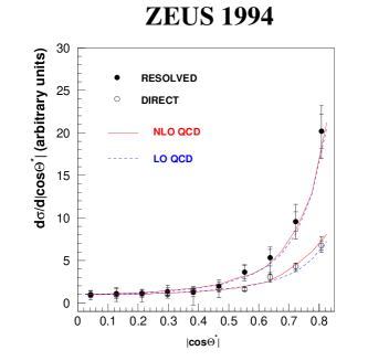
Figure 22: Dijet angular distribution, from Ref. $\!{}^{{\bf?}}$.

The expected difference in the distribution as $|\cos\theta^{*}|\to 1$ between the ‘direct’ and ‘resolved’ samples is clearly seen, and in both cases there is good agreement with NLO QCD predictions.

Another interesting result concerns the first quantitative measurements at HERA of large $p_{T}$ photon photoproduction $\!{}^{{\bf?}}$. At leading order, this proceeds via the Compton scattering of a photon off a quark:

$$d\sigma\;\sim\;\sum_{q}e_{q}^{4}\;q^{p}\otimes\hat{\sigma}(\gamma q\to\gamma q)+\ldots\;.$$ (35)

At higher orders there are also contributions from resolved processes such as $qg\to\gamma q$. Fig. 23 shows the distribution in $x_{\gamma}$ for direct photon events from the ZEUS collaboration. A clear excess at large $x_{\gamma}$ is seen, signalling the direct Compton scattering process. The interesting feature of the Compton process is that it is proportional to the fourth power of the quark charge, and therefore probes a different linear combination of quark distributions in the proton than the deep inelastic structure function $\!{}^{{\bf?}}$. The photon angular distribution of the Compton process should again exhibit a characteristic $(1-|\cos\theta^{*}|)^{-1}$ form at small angles.

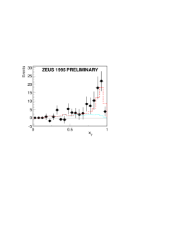
Figure 23: Distribution in $x_{\gamma}$ of prompt photon events at HERA, from Ref. $\!{}^{{\bf?}}$.

6 Diffractive deep inelastic scattering

The observation of ‘diffractive’ deep inelastic events with a large rapidity gap $\!{}^{{\bf?}}$ has spawned a new field of interest at HERA in the last few years. At this Workshop, as last year, there was much lively discussion about the measurement and interpretation of these events.

The focus of attention so far is the diffractive structure function $F_{2}^{D}$. This is obtained from a subclass of DIS events in which there is a large rapidity gap (H1, ZEUS) or from the observed excess of events with small $M_{X}$ (the invariant mass of hadrons in the detector) over the expected non-exponentially-suppressed non-diffractive contribution (ZEUS). The ZEUS collaboration have also identified energetic, small-angle protons in the Leading Proton Spectrometer (LPS), consistent with the interpretation that $ep\to epX$ is the underlying process.

The forward proton momentum can be parametrized in terms of the (small) momentum transfer $t$ and the longitudinal momentum fraction $1-x_{p}\approx 1$. One can then define a diffractive structure function $F_{2}^{D(4)}(x_{\rm Bj},Q^{2};x_{p},t)$ or equivalently $F_{2}^{D(4)}(\beta,Q^{2};x_{p},t)$ where $\beta=x_{\rm Bj}/x_{p}\simeq Q^{2}/(Q^{2}+M_{X}^{2})$. If $t$ is unmeasured and therefore integrated over, one can define a corresponding $F_{2}^{D(3)}(\beta,Q^{2};x_{p})$ function. The crucial experimental observations are that $F_{2}^{D(4)}$ is a leading twist structure function, indicating deep inelastic scattering off point-like objects, and that there is an approximate factorization property:

$$F_{2}^{D(3)}\sim x_{p}^{-n}{\cal F}(\beta,Q^{2})\;.$$ (36)

At the Paris Workshop last year, the values $n=1.19\pm 0.06({\rm stat.})\pm 0.07({\rm sys.})$ (H1 $\!{}^{{\bf?}}$) and $n=1.30\pm 0.08({\rm stat.}){+0.08\atop-0.14}({\rm sys.})$ (ZEUS $\!{}^{{\bf?}}$) were reported. This year, with new data, H1 have measured $n$ as a function of $\beta$ and $Q^{2}$, see Fig. 24.

Figure 24: Measurement of the parameter $n$, where $F_{2}^{D(3)}\sim x_{p}^{-n}$, from H1 $\!{}^{{\bf?}}$.

A clear dependence on $\beta$ (but not on $Q^{2}$) is observed. ZEUS have also reported new values: $n=1.46\pm 0.10$ from $F_{2}^{D(2)}$ defined by the $M_{X}$ distribution $\!{}^{{\bf?}}$, and $n=1.28\pm 0.17$ from the LPS data $\!{}^{{\bf?}}$. Note that these are not in contradiction, since the $\langle\beta\rangle$ averages are different for the two samples. However, as last year, they do appear to be slightly larger than the H1 values.

The most attractive theoretical interpretation of these diffractive DIS events is that they correspond to the structure function of the pomeron (${\cal P}$), rather than the proton (for a review see Ref. $\!{}^{{\bf?}}$). In its simplest version, this model would predict

$$F_{2}^{D(4)}(\beta,Q^{2};x_{p},t) = f_{{\cal P}}(x_{p},t)\;F_{2}^{{\cal P}}(\beta,Q^{2})\;,$$

$$\quad f_{{\cal P}}(x_{p},t)=F_{{\cal P}}(t)x_{p}^{2\alpha_{{\cal P}}(t)-1}\;, F_{2}^{{\cal P}}(\beta,Q^{2})=\beta\sum_{q}e_{q}^{2}q_{{\cal P}}(\beta,Q^{2})\;,$$ (37)

i.e. a factorized structure function with $n\approx 2\alpha_{{\cal P}}(0)-1\approx 1.16$. This model is based on the notion of ‘parton constituents in the pomeron’ first proposed by Ingelman and Schlein $\!{}^{{\bf?}}$ and supported by data from UA8. In such a model, a modest amount of factorization breaking could be accommodated by invoking a sum over Regge trajectories, each with a different intercept and structure function:

$$F_{2}^{D(4)}(\beta,Q^{2};x_{p},t)=\sum_{{\cal R}}\;F_{{\cal R}}(t)x_{p}^{2\alpha_{{\cal R}}(t)-1}\;F_{2}^{{\cal R}}(\beta,Q^{2})\;,$$ (38)

which would yield an effective $n$ which depends on $\beta$ but is approximately independent of $Q^{2}$.

The above approach has been put on a firmer theoretical footing in Ref. $\!{}^{{\bf?}}$, where the general concept of ‘diffractive parton distributions’ is introduced. In particular it is shown that an operator product definition exists, and that the diffractive distributions should satisfy DGLAP evolution equations. There has been a number of analyses based on DGLAP fits to diffractive structure function data in the last year. At this Workshop the H1 collaboration has presented a new measurement of $F_{2}^{(D)}$ (i.e. integrated over both $x_{\cal P}$ and $t$) and a new NLO QCD fit, see Fig. 25.

Figure 25: The diffractive structure function $F_{2}^{(D)}$ measured by H1 $\!{}^{{\bf?}}$, together with the result of a NLO QCD fit.

The resulting parton distributions at $Q^{2}=5\;{\rm GeV}^{2}$ are shown in Fig. 26.

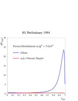
Figure 26: Parton distributions obtained from the fit to the data shown in Fig. 25 $\!{}^{{\bf?}}$.

Evidently the ‘pomeron’ (more precisely, the aggregate of the colour-singlet exchanges in Eq. (38)) is a predominantly gluonic object. Although the structure function only directly measures the quark distributions, a very hard gluon distribution is needed to give an approximate scaling (in $Q^{2}$) behaviour at large $\beta$, see Fig. 25.

From a purely phenomenological point of view, the above model has many attractive features. It enables predictions to be made, for example for the charm content of the diffractive structure function $\!{}^{{\bf?}}$ and the rate of jet production in diffractive DIS events $\!{}^{{\bf?}}$. With a further assumption of universality of diffractive parton distributions, which lacks any theoretical proof at present however, one can make quantitative predictions for diffractive hard scattering processes in photon-hadron and hadron-hadron collisions $\!{}^{{\bf?},{\bf?}}$.

Finally, we should mention a different approach to diffractive deep inelastic scattering based on perturbative QCD. In the microscopic colour dipole model $\!{}^{{\bf?}}$, a generalized ‘BFKL’ gluon ladder interacts with the $q\bar{q}$ Fock state of the virtual photon. In this model many features of $F_{2}^{D}$ can be predicted from QCD perturbation theory. The most striking features are the breaking of the Regge factorization of Eq. (37), and the qualitative differences between the longitudinal and transverse structure functions $\!{}^{{\bf?}}$:

$$F_{T}^{D}\sim g^{2}\left(x_{p},{m_{q}^{2}\over 1-\beta}\right)\;,\quad F_{L}^{D}\sim{1\over Q^{2}}g^{2}\left(x_{p},{Q^{2}\over 4}\right)\;.$$ (39)

Note that there is no $x_{p}-(\beta,Q^{2})$ factorization, and also no DGLAP evolution as $\beta\to 1$ at high $Q^{2}$, where $F_{T}^{D}$ dominates. The $x_{p}$ dependence is determined by the $x\to 0$ behaviour of the gluon distribution, and is generally steeper than the behaviour predicted by the simple (soft) pomeron model. For heavy quarks, a perturbatively hard scale is set by $m_{q}^{2}$, and infra-red safe predictions can be made from first principles  $\!{}^{{\bf?},{\bf?}}$. Like the soft pomeron model, the pQCD model is so far in good agreement with the data. Once again the conclusion is obvious: more data, not only on $F_{2}^{D(4)}(\beta,Q^{2};x_{p},t)$ but also on $F_{L}^{D}$, charm and jet production, are urgently needed to discriminate between these different approaches.

7 Conclusions

At this Workshop we have seen significant progress in almost all aspects of deep inelastic scattering physics. Advances in experimental measurements are matched by advances in theoretical calculations, and our understanding of the short-distance structure of hadrons steadily improves as a result. However, each new Workshop inevitably produces new questions to be answered. Some of these have been discussed in this summary: for example, why does NLO DGLAP work so well even at small $x$ and $Q^{2}$ values, can we push the uncertainty in the gluon distribution below the $10\%$ level, is there a systematic difference between the deep inelastic $\alpha_{s}$ values extracted from high and low $x$, how can the polarized gluon distribution be directly measured, and can the deep inelastic diffractive data really be understood in a simple ‘pomeron parton model’ or will the explicit factorization-breaking properties of the pQCD model be revealed? We look forward to some answers next year!

References

References

- [1] H1 collaboration: M. Klein, these Proceedings.
- [2] ZEUS collaboration: R. Yoshida, these Proceedings.
- [3] ZEUS collaboration: Q. Zhu, these Proceedings.
- [4] E665 collaboration: T. Carroll, these Proceedings.
- [5] A. Donnachie and P.V. Landshoff, Z. Phys. C61 (1994) 139.
- [6] M. Glück, E. Reya and A. Vogt, Z. Phys. C67 (1995) 433; A. Vogt, these Proceedings.
- [7] B. Badelek and J. Kwiecinski, Phys. Lett. B295 (1992) 263.
- [8] A. Levy, these Proceedings.
- [9] A. Milsztajn and M. Virchaux, Phys. Lett. B274 (1992) 221.
- [10] NMC collaboration: E.M. Kabuß, these Proceedings.
- [11] R.K. Ellis, W.J. Stirling and B.R. Webber, QCD and Collider Physics, Cambridge University Press, 1996.
- [12] R.G. Roberts, these Proceedings; A.D. Martin, R.G. Roberts and W.J. Stirling, Durham preprint DTP/96/44 (1996).
- [13] CTEQ collaboration: W.-K. Tung, these Proceedings.
- [14] H1 collaboration: U. Bassler, these Proceedings.
- [15] A.D. Martin, R.G. Roberts and W.J. Stirling, Phys. Lett. B354 (1995) 155.
- [16] A. De Rujula, S.L. Glashow, H.D. Politzer, S.B. Treiman, F. Wilczek and A. Zee, Phys. Rev. D10 (1974) 1649.
- [17] R.D. Ball and S. Forte, Phys. Lett. B335 (1994) 77; B336 (1994) 77.
- [18] S. Forte, these Proceedings.
- [19] R.G. Roberts, private communication.
- [20] See the contributions by J. Blümlein, S. Catani, S. Forte and R.S. Thorne to these Proceedings.
- [21] S. Catani and F. Hautmann, Nucl. Phys. B427 (1994) 475.
- [22] R.D. Ball and S. Forte, Phys. Lett. B351 (1995) 513.
-
[23]
E.A. Kuraev, L.N. Lipatov and V.S. Fadin, Phys. Lett.
B60 (1975) 50; Sov. Phys. JETP
44 (1976) 433; 45 (1977) 199.
Ya.Ya. Balitsky and L.N. Lipatov, Sov. J. Nucl. Phys. 28 (1978) 822. - [24] S. Catani, M. Ciafaloni and F. Hautmann, Phys. Lett. B242 (1990) 97; Nucl. Phys. B366 (1991) 657.
- [25] A.D. Martin, these Proceedings.
- [26] J. Kwiecinski, A.D. Martin and P.J. Sutton, Durham preprint DTP/96/02 (1996); see also Ref. .
- [27] See the contributions by A. De Roeck and V. Del Duca to these Proceedings.
- [28] R.C.E. Devenish and A.D. Martin, these Proceedings.
- [29] H1 collaboration: preprint DESY 96-093 (1996), see also Ref. .
-
[30]
CDF collaboration: C.E. Pagliarone, these Proceedings.
D0 collaboration: D. Elvira, these Proceedings. - [31] A.D. Martin, these Proceedings.
- [32] D. Graudenz, Phys. Rev. D49 (1994) 3291.
- [33] E. Mirkes and D. Zeppenfeld, Madison preprint MADPH-95-916 (1995); E. Mirkes, these Proceedings.
- [34] H1 collaboration: K. Rosenbauer, these Proceedings.
- [35] ZEUS collaboration: J. Repond, these Proceedings.
- [36] M.G. Ryskin, Z. Phys. C37 (1993) 89.
- [37] M.G. Ryskin, R.G. Roberts, A.D. Martin and E.M. Levin, Durham preprint DTP/95/96 (1995).
- [38] L. Frankfurt, W. Koepf and M. Strikman, Tel Aviv preprint TAUP-2290-95 (1995).
- [39] A.D. Martin, these Proceedings.
- [40] H1 collaboration: S. Aid et al., preprint DESY-96-046 (1996).
- [41] E. Eichten, I. Hinchliffe, K. Lane and C. Quigg, Rev. Mod. Phys. 56 (1984) 579.
- [42] A. Bodek, these Proceedings.
- [43] CCFR collaboration: P.Z. Quintas et al., Phys. Rev. Lett. 71 (1993) 1307.
- [44] CCFR-NuTeV collaboration: D.A. Harris et al., in Proc. 30th Rencontres de Moriond, Meribel les Allues, France, ed. J. Trân Thanh Vân, Editions Frontières, Gif sur Yvette (1996).
- [45] J. Ellis and M. Karliner, Phys. Lett. B341 (1995) 397.
-
[46]
H1 collaboration: T. Ahmed et al., Phys. Lett.
B346 (1995) 415.
ZEUS collaboration: M. Derrick et al., Phys. Lett. B363 (1995) 201. - [47] R.D. Ball and S. Forte, Phys. Lett. B358 (1995) 365.
- [48] R.D. Ball, these Proceedings.
- [49] H1 collaboration: I. Park, these Proceedings.
- [50] SMC collaboration: A. Witzmann, L.B. Betev, M. Rodriguez, these Proceedings.
- [51] SLAC-E143 collaboration: S. Rock, these Proceedings.
- [52] HERMES collaboration: M. Vetterli, D. de Schepper, K. Ackerstaff, these Proceedings.
- [53] SLAC-E142 collaboration: D.L. Anthony et al., Phys. Rev. Lett. 71 (1993) 959.
-
[54]
R. Mertig and W.L. van Neerven, Z. Phys. C70 (1996) 637.
W. Vogelsang, Rutherford Laboratory preprint RAL-TR-95-071 (1995), and these Proceedings. - [55] M. Glück, E. Reya, M. Stratmann and W. Vogelsang, Dortmund preprint DO-TH 95-13 (1995).
- [56] R.D. Ball, S. Forte and G. Ridolfi, preprint CERN-TH/95-266 (1995), and these Proceedings.
- [57] T. Gehrmann and W.J. Stirling, Phys. Rev. D53 (1996) 6100, and these Proceedings.
- [58] E. Mirkes, these Proceedings.
- [59] B.I. Ermolaev, S.I. Manayenkov and M.G. Ryskin, preprint DESY-95-017 (1995).
- [60] J. Blümlein and A. Vogt, Phys. Lett. B370 (1996) 149.
- [61] J. Bartels, B.I. Ermolaev and M.G. Ryskin, Z. Phys C70 (1996) 273; preprint DESY-96-025 (1996), and these Proceedings.
- [62] J. Blümlein and A. Vogt, preprint DESY-96-041 (1996), and these Proceedings.
- [63] ZEUS collaboration: L. Feld, these Proceedings.
- [64] ZEUS collaboration: P.J. Bussey, these Proceedings.
- [65] A.C. Bawa, M. Krawczyk and W.J. Stirling Z. Phys. C50 (1991) 293.
-
[66]
ZEUS collaboration: M. Derrick et al., Phys. Lett. B315 (1993) 481;
B332 (1994) 228; B338 (1994) 483.
H1 collaboration: T. Ahmed et al., Nucl. Phys. B429 (1994) 477. - [67] H1 collaboration: T. Ahmed et al., Phys. Lett. B348 (1995) 681.
- [68] ZEUS collaboration: M. Derrick et al., Z. Phys. C68 (1995) 569.
- [69] H1 collaboration: P.R. Newman, these Proceedings.
- [70] ZEUS collaboration: H. Kowalski, these Proceedings.
- [71] ZEUS collaboration: E. Barberis, these Proceedings.
- [72] P.V. Landshoff, these Proceedings.
- [73] G. Ingelman and P. Schlein, Phys. Lett. B152 (1985) 256.
- [74] A. Berera and D.E. Soper, Phys. Rev. D53 (1996) 6162, and these Proceedings.
- [75] T. Gehrmann and W.J. Stirling, Z. Phys. C70 (1996) 89.
- [76] H1 collaboration: J. Theissen, these Proceedings.
- [77] ZEUS collaboration: J. Puga Ortiz, these Proceedings.
- [78] Z. Kunszt and W.J. Stirling, these Proceedings.
- [79] M. Genovese, N.N. Nikolaev and B.G. Zakharov, J. Exp. Theor. Phys. 81 (1995) 625; Torino preprint DFTT 77/95, and these Proceedings.