Top quark loop corrections to the decay $H^{+}\rightarrow h^{0}W^{+}$
in the Two Higgs Doublet Model

Abstract

We calculate the decay width for the process $H^{+}\rightarrow h^{0}W^{+}$ up to order $g^{4}$ in the framework of the Two Higgs Doublet Model. We argue that for some reasonable choice of the free parameters the contribution from the one-loop graphs can be as large as 80%.

1 Introduction

Despite the enormous success of the $SU(2)\otimes U(1)$ Electroweak theory, the fundamental mechanism responsible for the gauge boson masses remains untested. This by itself justifies the study of extensions of the minimal model. Among these various extensions the most important one is the two-Higgs doublet model (2HDM). In fact, even without considering supersymmetry, the existence of more than one generation of scalar fields is a possibility that ought to be explored. (See ref.[1] for a general review).

The existence of charged scalar particles $H^{+},H^{-}$ is the cleanest signature for the 2HDM. so it is important to study the production and decays of these particles. The production of $H^{+}H^{-}$ is kinematically suppressed in lepton colliders. On the contrary, in hadron colliders one could produce a substantial number of charged Higgs via the reaction $g\bar{b}\rightarrow H^{+}\bar{t}$ [2]. After the production, the dominant decay channel is $H^{+}\rightarrow t\bar{b}$ which, unfortunately, due to the large QCD background, makes the detection very difficult. For this reason, the alternative channel $H^{+}\rightarrow h^{0}W^{+}$, where $h^{0}$ is the lightest of the neutral Higgs bosons, could be very important. The calculation of the top quark loops to the decay width of the process $H^{+}\rightarrow W^{+}h^{0}$ is our aim.

Previously, some of us [3, 4] have discussed the vacuum stability and the renormalization of the most general 2HDM with CP conservation. There are two kinds of potentials with only CP invariant minima and both dependent on seven real parameters. In here, we work with the following potential, denoted by $V(I)$ in ref.[2],

$$V=-\mu_{1}^{2}x_{1}-\mu_{2}^{2}x_{2}+\lambda_{1}x_{1}^{2}+\lambda_{2}x_{2}^{2}+\lambda_{3}x_{3}^{2}+\lambda_{4}x_{4}^{2}+\lambda_{5}x_{1}x_{2}$$ (1)

where

$$x_{1}=\phi_{1}^{+}\phi_{1},\qquad x_{2}=\phi_{2}^{+}\phi_{2},\qquad x_{3}=\mbox{Re}(\phi_{1}^{+}\phi_{2}),\qquad x_{4}=\mbox{Im}(\phi_{1}^{+}\phi_{2})$$ (2)

and $\phi_{i}$ are two complex scalar doublets with hypercharge Y=1.

To renormalize the model using on-shell prescription the seven real parameters of $V$ are replaced by the square of the vacuum expectation value $v^{2}=v_{1}^{2}+v_{2}^{2}$, the masses of the Higgs particles, $H^{+}$, $H^{-}$, $H^{0}$, $h^{0}$ and $A^{0}$, the ratio $\frac{v_{2}}{v_{1}}\equiv\tan\beta$ and the angle $\alpha$, which rotates the mass eigenstates $H^{0}$ and $h^{0}$ to the $SU(2)$ eigenstates.

2 The decay width

Let $q$ denote the 4-momentum of $H^{+}$, $q^{\prime}$ the 4-momentum of $h^{0}$ and $p=q-q^{\prime}$ the 4-momentum of $W^{+}$. Thus, at tree level the decay amplitude $H^{+}\rightarrow h^{0}W^{+}$ is

$$T=\varepsilon^{*}_{\mu}\Gamma_{0}^{\mu}$$ (3)

with

$$\Gamma_{0}^{\mu}=\frac{g}{2}\cos(\beta-\alpha)(q+q^{\prime})^{\mu}$$ (4)

This, in turn leads to the following expression to the decay width

$$\Gamma=\frac{g^{2}\cos^{2}(\beta-\alpha)}{64\,\pi M_{W}^{2}M_{H^{+}}^{3}}\,\left[\left(M_{H^{+}}^{2}-M_{h^{0}}^{2}-M_{W}^{2}\right)^{2}-4M_{h^{0}}^{2}M_{W}^{2}\right]^{\frac{3}{2}}$$ (5)

At one-loop order, the renormalized $H^{+}H^{0}W^{+}$ vertex $\Gamma^{\mu}_{1ren}$ is represented in fig. 1. Diagrams a) and b) are the unrenormalized proper vertex and its counterterm, respectively, and the remaining diagrams, where the crossed circles represent the renormalized two-point Greens functions, are corrections to the external legs.

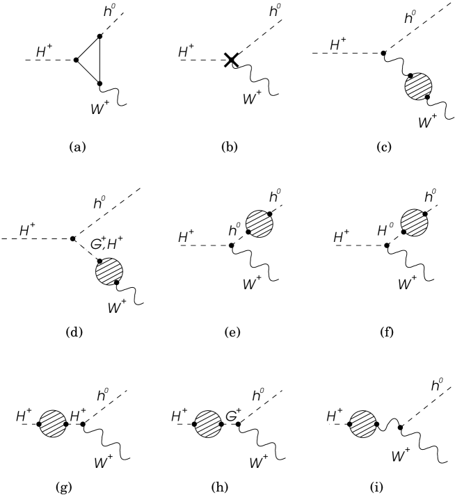
Figure 1: Feynman graphs at one-loop level

Using the on-shell renormalization prescription all these diagrams vanish, assuming, as we do, that the particles are on-shell. Without giving the details that can be found elsewhere [4, 5], let us simply make a few comments. Clearly the on-shell condition implies that diagram c) vanishes. Similarly, diagram d) is also zero, because, for an on-shell $W^{+}$, the mixed self-energy is proportional to $p^{\mu}$ and $\varepsilon\cdot p=0$.

Under renormalization, particles with the same quantum numbers get mixed. So the relation between the bare fields $h^{0}$ and $H^{0}$, for instance, and the renormalized ones is a matrix, i.e.,

$$\left[\begin{array}[]{l}H^{0}\\ h^{0}\end{array}\right]_{0}\,=\,\left[\begin{array}[]{ll}Z^{\frac{1}{2}}_{H^{0}H^{0}}&Z^{\frac{1}{2}}_{H^{0}h^{0}}\\ Z^{\frac{1}{2}}_{h^{0}H^{0}}&Z^{\frac{1}{2}}_{h^{0}h^{0}}\end{array}\right]\left[\begin{array}[]{l}H^{0}\\ h^{0}\end{array}\right],\quad M_{i0}^{2}=M_{i}^{2}+\delta M_{i}^{2},\quad i=H^{0},h^{0}.$$ (6)

Then the wave function renormalization constants are fixed by the following conditions, imposed on the renormalized self-energies

$$\left.\Sigma_{R}^{H^{0}H^{0}}(p^{2})\right|_{p^{2}=M_{H^{0}}^{2}}\,=\,0$$ (7a)

and

$$\left.\Sigma_{R}^{H^{0}h^{0}}(p^{2})\right|_{p^{2}=M_{h^{0}}^{2}}\,=\,0$$ (7b)

These conditions guarantee that diagrams e) and f) vanish, Similar conditions can be imposed on the renormalized self-energy of the charged Higgs and on the mixing self-energy $H^{+}G^{+}$ between the charged Higgs and the Goldstone boson $G^{+}$, i.e.

$$\left.\Sigma_{R}^{H^{+}H^{+}}(p^{2})\right|_{p^{2}=M_{H^{+}}^{2}}\,=\,0$$ (8a)

and

$$\left.\Sigma_{R}^{H^{+}G^{+}}(p^{2})\right|_{p^{2}=0}\,=\,0.$$ (8b)

This, in turn, guarantees that diagrams g) and h) are also zero. Now, the counterterm for the $H^{+}W^{+}$ is given without any further constraint by

$$-\frac{i}{2}p^{\mu}M_{W}\delta Z_{G^{+}H^{+}}$$ (9)

where $\delta Z_{G^{+}H^{+}}$ is the off diagonal term for the wave function renormalization matrix of the charged scalars. Then, the vanishing of diagram i) provides a consistency check of the calculation.

For the sake of completeness, we write the counterterm Lagrangian $\mbox{\cal{L}}_{CT}$ for the CP-even charged Higgs sector, namely

$$\mbox{\large\cal L}_{C.T.} = -\delta m_{H^{0}}^{2}+(q^{2}-m_{H^{0}}^{2})\delta Z_{H^{0}H^{0}}-\delta_{H^{0}H^{0}}$$

$$-\delta m_{h^{0}}^{2}+(q^{2}-m_{h^{0}}^{2})\delta Z_{h^{0}h^{0}}-\delta_{h^{0}h^{0}}$$

$$+\frac{1}{2}(q^{2}-m_{H^{0}}^{2})\delta Z_{H^{0}h^{0}}+\frac{1}{2}(q^{2}-m_{h^{0}}^{2})\delta Z_{h^{0}H^{0}}-\delta_{H^{0}h^{0}}$$

$$-\delta m_{H^{+}}^{2}+(q^{2}-m_{H^{+}}^{2})\delta Z_{H^{+}H^{+}}-\delta_{H^{+}H^{+}}$$

$$+q^{2}\delta Z_{G^{+}G^{+}}-\delta_{G^{+}G^{+}}$$

$$+\frac{1}{2}(q^{2}-m_{H^{+}}^{2})\delta Z_{H^{+}G^{+}}+\frac{1}{2}q^{2}\delta Z_{G^{+}H^{+}}-\delta_{H^{+}G^{+}}$$

where

$$\delta_{H^{0}h^{0}} = \frac{\sin 2\alpha}{v\sin 2\beta}\left(T_{H}\sin(\alpha-\beta)+T_{h}\cos(\alpha-\beta)\right)$$

$$\delta_{H^{0}H^{0}} = \frac{2}{v\sin 2\beta}\left(T_{H}(\cos^{3}\alpha\sin\beta+\sin^{3}\alpha\cos\beta)\right.$$

$$\qquad\qquad\qquad\left.+T_{h}\sin\alpha\cos\alpha\sin(\alpha-\beta)\right)$$

$$\delta_{h^{0}h^{0}} = \frac{2}{v\sin 2\beta}\left(T_{H}\sin\alpha\cos\alpha\cos(\alpha-\beta)\right.$$

$$\qquad\qquad\qquad\left.+T_{h}(\cos^{3}\alpha\cos\beta-\sin^{3}\alpha\sin\beta)\right)$$

$$\delta_{H^{+}G^{+}} = \frac{1}{v}\left(T_{H}\sin(\alpha-\beta)+T_{h}\cos(\alpha-\beta)\right)$$ (11)

$$\delta_{G^{+}G^{+}} = \frac{1}{v}\left(T_{H}\cos(\alpha-\beta)-T_{h}\sin(\alpha-\beta)\right)$$

$$\delta_{H^{+}H^{+}} = \frac{2}{v\sin 2\beta}\left((\cos^{3}\beta\sin\alpha+\sin^{3}\beta\cos\alpha)T_{H}\right.$$

$$\qquad\qquad\qquad\left.+(\cos^{3}\beta\cos\alpha-\sin^{3}\alpha\sin\beta)T_{h}\right)$$

$T_{H}$ and $T_{h}$ are the tadpole counterterms, fixed by the renormalization condition on the 1-particle Green function, as shown in fig.2.

Figure 2: tadpole renormalization condition.

The calculation of diagram a) is standard. There are several particles that can be included in the loop. However, in here we consider quark loops, assumed to be dominant due to the large top quark mass. Notice that this subset has to be finite by itself.

Diagram b) of fig. 1 has two main contributions. The first one comes from the parameter variation on the tree level coupling $H^{+}H^{0}W^{+}$ and it is

$$i\frac{g}{2}\,\cos(\beta-\alpha)\,(q+q^{\prime})^{\mu}\,\left[\;\frac{\delta g}{g}\;+\;\frac{1}{2}\delta Z_{H^{+}H^{+}}\;+\;\frac{1}{2}\delta Z_{h^{0}h^{0}}\right.$$ (12)

$$\qquad\qquad\qquad\qquad\qquad\quad\left.+\;\frac{1}{2}\delta Z_{WW}\;-\;\tan(\beta-\alpha)\delta(\beta-\alpha)\;\right]$$

The second contribution is due to the existence of other tree level couplings $H^{+}H^{0}W^{+}$ and $G^{+}h^{0}W^{+}$, that, due to wave function mixing, induced the vertex that we want, namely:

$$i\frac{g}{2}\,\sin(\beta-\alpha)\,(q+q^{\prime})^{\mu}\,\left[\frac{1}{2}\delta Z_{H^{+}G^{+}}-\frac{1}{2}\delta Z_{h^{0}h^{0}}\right]$$ (13)

Besides $\delta(\beta-\alpha)$, all parameter in eq.(12) and (13) are already fixed. In fact, like in the minimal standard model, $\delta g$ id fixed by the photon electron vertex. The interesting point to notice is that one requires a $\delta(\beta-\alpha)$ to obtain a renormalized finite result. In principle, in this model $\beta$ and $\alpha$ are two physical parameters that could be fixed independently. However, for illustrative purpose we have decided to renormalize the angle $(\beta-\alpha)$ using the similar process $H^{+}\rightarrow H^{0}W^{+}$ which at tree level is proportional to $\sin(\beta-\alpha)$. Then, $\delta(\beta-\alpha)$ is fixed imposing that the one-loop $H^{+}H^{0}W^{+}$ vertex vanishes for $q^{2}=M_{H^{+}}^{2}$, $q^{\prime 2}=M_{H^{0}}^{2}$ and $p^{2}=M_{W}^{2}$, i.e.

$$\left.\Gamma^{\mu}_{1ren}\left(H^{+}H^{0}W^{+}\right)\right|_{(M_{H^{+}}^{2},M_{H^{0}}^{2},M_{W}^{2})}\,=\,0$$ (14)

This implies that, in this model, without further measurements, the decay $H^{+}\rightarrow H^{0}W^{+}$ fixes the parameter $(\beta-\alpha)$ and $H^{+}\rightarrow h^{0}W^{+}$ checks the consistency of the theory at one-loop level. Clearly this implies a kinematical bound

$$M_{H^{+}}^{2}>M_{W}^{2}+M_{H^{0}}^{2}$$

It is interesting to point out that our calculation is similar to the study of the radiative decay $H^{+}\rightarrow\gamma W^{+}$ [6]. In that case, the main one-loop corrections are also due to top quark loops, but there is a major difference. As a consequence of the electromagnetic $U(1)$ invariance, there is no tree level contribution. Then, the proper vertex counterterm ( the equivalent of fig 1b) ) cancels with the counterterms of the external legs diagrams [7]. This means that the calculation can be done simply by summing all unrenormalized reducible and irreducible diagrams. This sum is finite and electromagnetic gauge invariant. On the contrary, the one-loop calculation for the decay width $H^{+}\rightarrow h^{0}W^{+}$ requires a detailed renormalization program for the 2HDM.

3 Results and discussion

For our numerical calculation we used a computer Maple[8] program[9]. All quark masses except $m_{t}=180$ GeV and $m_{b}=4.1$ GeV have been neglected. The values of the remaining parameters were taken from Particle Data Group[10], the CKM matrix element $V_{tb}$ was set equal to one and the angles $\beta$ and $\alpha$ were varied in the range $0<\beta<\frac{\pi}{2}$ and $-\frac{\pi}{2}<\alpha<\frac{\pi}{2}$. According to tree unitarity analysis [11] the Higgs boson masses are bounded from above as $M_{H^{+}}<870$ GeV, $M_{H^{0}}<710$ GeV and $M_{h^{0}}<500$ GeV. In our numerical examples we respect these bounds but no further constraints are imposed.

Figure 3: Decay width as a function of $\alpha$. One-loop means the contribution from the tree level plus the contribution from the one-loop graphs.

In fig. 3 we show the decay width for $M_{H^{+}}=600$ GeV, $M_{H^{0}}=500$ GeV, $M_{h^{0}}=400$ GeV and $\tan\beta=2$ as a function of $\alpha$. The dotted curve gives the tree level result, while the full curve includes also top quark loops. Depending on the value of $\alpha$, the one-loop result varies between 20% and 60% of the tree level result. Obviously this enhancement depends on the values of the parameters. The dashed curve shows the relative importance of the one-loop contribution in percentage. This curve grows to infinity when $\alpha=\beta-\frac{\pi}{2}$ which corresponds to a zero tree level result.

Figure 4: Decay width as a function of $\beta$.

The range that we have indicated is representative of reasonable values for the angles. However, very large enhancement can be obtained for small values of $\beta$. This is shown in fig. 4, where we plot the decay width as a function of $\beta$ for $M_{H^{+}}=500$ GeV, $M_{H^{0}}=200$ GeV, $M_{h^{0}}=100$ GeV and $\alpha=0.3\pi$. Notice that a small $\beta$ implies a very large coupling between the Higgs and the top quark. Obviously, at some point, perturbation theory breaks down.

Figure 5: Decay width as a function of $M_{H^{+}}$ for $\alpha=-0.1\pi$(dashed and dotted curve) and $\alpha=0.3\pi$(solid).

Finally in fig. 5 we show the variation of the decay width with the mass of the charged Higgs boson, for $M_{H^{0}}=150$ GeV, $M_{h^{0}}=100$ GeV, $\tan\beta=2$ and two values for $\alpha$, $\alpha=0.3\pi$ and $\alpha=-0.1\pi$. As we would expect, the decay width of $H^{+}\rightarrow h^{0}W^{+}$ grows with $M_{H^{+}}$ and the relative importance of the quark loop corrections also grows with $M_{H^{+}}$. In this figure, the right hand scale corresponds to the dashed and dotted curves which are the tree level(dotted) and tree plus one-loop (dashed) for $\alpha=-0.1\pi$. The solid curve has the scale on the left side and represents the tree level plus one-loop result for $\alpha=0.3\pi$. On the same scale, the tree level curve is almost coincident with the solid curve and for this reason it is not shown. We have also studied the dependence of the result in $M_{h^{0}}$. Leaving aside the phase space dependence, which is most important at threshold, the dependence is mild, and there is no point showing it. The same happens with the dependence on $M_{H^{0}}$.

The comparison of these two cases illustrates the following qualitative argument: the width is larger when $\alpha\approx\beta$, but in this case the loop corrections are smaller (about 1% for any value of $M_{H^{+}}$), on contrary, when $\beta$ and $\alpha$ are different the overall result is smaller but the quark loop corrections grow in relative importance, reaching in some cases 80% of the tree level contribution.

References

[1] J. Gunion, H. Haber, G. Kane, S. Dawson
The Higgs Hunter’s Guide, Addison Wesley (1990)
[2] J. Gunion, H. Haber, F. Paige, Wu-ki Tung
and S.S.D Willenbrock
Nucl. Phys. B294 (1987) 621
[3] J. Velhinho, R. Santos and A. Barroso
Phys. Lett. B322 (1994) 213
[4] A. Barroso and R. Santos, in preparation
[5] K. Aoki, Z. Hioki, R. Kawabe, M. Konuma, T. Muta
Suppl. Prog. Theor. Phys. 73 (1982) 1
[6] S. Raychaudhuri and A. Raychaudhuri,
Phys. Lett B297 (1992) 159
[7] J. Soares and A. Barroso
Phys.Rev. D39 (1989) 1973
[8] B. W. Char, K. O. Geddes, G. H. Gonnet, B. L. Leong,
M. B. Monagan, S. M. Watt: Maple V, Springer (1991)
[9] L. Brücher, J. Franzkowski, D. Kreimer.
Computer Physics Communication 85 (1995) 153-165
[10] L. Montanet et al.
Phys. Rev. D 50, 1173 (1994) and 1995 off-year partial
update for the 1996 edition
( available via WWW http://pdg.lbl.gov/ )
[11] S. Kanemura, T. Kubota and E. Takasugi,
Phys. Lett. B 313, 155 (1993);
J. Maalampi, J. Sirkka, I. Vilja,
Phys. Lett. B 265, 371 (1991).