SAGA–HE–108

August 16, 1996

$CP$ Violation and Baryogenesis
at the Electroweak Phase Transition

Koichi Funakubo

Department of Physics, Saga University, Saga 840

Abstract

We report a recent attempt to relate $CP$ violation in the electroweak theory with two Higgs doublets to the baryon asymmetry generated at the electroweak phase transition, after surveying the scenario of the electroweak baryogenesis.

1 Introduction

The evolution of the universe is well described by the standard hot big bang model and its early stage offers a common field for particle physics and astrophysics[1]. Not only have various observations in laboratories been clues to understand what occurred in the early universe, but new ideas have also led to resolutions of the problems concerning very early universe; e.g., grand unified models with strong first-order phase transitions led to the idea of inflation, and dark matter may be explained by new physics, which will be examined in the near future. On the other hand, astrophysical observations give constraints on models of particle physics which cannot be obtained from accelerator experiments[2]. The baryon asymmetry of the universe (BAU) is among these topics.

The BAU is one of the most obvious facts[1]: we do not observe any antimatter in our solar system, and high energy cosmic rays, which contain a small amount of anti-protons consistent as secondary products, are evidence of the baryon asymmetry on the galactic scale. The absence of hard $\gamma$ rays, which would be emitted on nucleon-antinucleon annihilation, from nearby clusters of galaxies, such as the Virgo cluster, implies that such a cluster consists of $(1\sim 100)M_{\rm galaxy}\simeq 10^{12\sim 14}M_{\odot}$ of either baryons or antibaryons only. While we have no evidence for baryon asymmetry on a larger scale, matter should be separated from antimatter on scale of, at least, $10^{12}M_{\odot}$. We characterize this manifest quantity by the ratio of the baryon number to entropy

$${{n_{B}}\over s}\equiv{{n_{b}-n_{\bar{b}}}\over s},$$ (1.1)

where $s$ is the entropy density and $n_{b}$($n_{\bar{b}}$) is the (anti)baryon number density. This remains constant in the absence of a baryon-number-changing process and entropy production, during the expansion of the universe. To explain the light-element abundances within the framework of the standard big-bang nucleosynthesis, it is required that $\eta\equiv n_{B}/n_{\gamma}=(1.5-6.3)\times 10^{-10}$[2]. As shown in Appendix A, the photon density $n_{\gamma}$ is related to $s$ by $s=7.04n_{\gamma}$ at present[1],  so that

$${{n_{B}}\over s}=(0.21-0.90)\times 10^{-10}.$$ (1.2)

This is very small but sufficient to form the present visible matter. Although one might think that matter and antimatter were separated on a scale of $10^{12}M_{\odot}$ in locally baryon-symmetric universe, the present BAU cannot be explained without any primordial asymmetry. The present baryons are those which survived the nucleon-antinucleon annihilation and which froze out at $T\simeq 20\mbox{MeV}$. Since starting from the baryon-symmetric universe $n_{b}/s\simeq n_{\bar{b}}/s\sim 7\times 10^{-20}$ after the freeze out, the BAU, which is about nine orders larger, could not be generated[1], To avoid this annihilation, suppose that some hypothetical mechanism separated nucleons and antinucleons before $T\simeq 38\mbox{MeV}$, when $n_{b}/s=n_{\bar{b}}/s\sim 8\times 10^{-11}$. At that time the matter contained in the causal region was only about $10^{-7}M_{\odot}\mathrel{<\kern-5.0pt<}10^{12}M_{\odot}$. Hence it is natural to assume that the universe had baryon asymmetry before it cooled down to $T\simeq 38\mbox{MeV}$.

To obtain the BAU starting from the symmetric universe, three conditions, first proposed by Sakharov[3], must be satisfied:

• baryon number violation,

• $C$ and $CP$ violation,

• departure from equilibrium.

Without condition (1), the symmetric universe remains baryon-symmetric, and it seems difficult to realize a locally asymmetric but globally symmetric universe, as we saw above. If $C$ and $CP$ were conserved, baryon number could not be generated in the symmetric universe. This is understood as follows. Suppose that the initial state of the universe is described by a density operator $\rho_{0}$ which is $C$- and $CP$-invariant. Since baryon number is odd under $C$ and $CP$, $\langle n_{B}\rangle_{0}={\rm Tr}[\rho_{0}n_{B}]=0$. If the hamiltonian of the system is $C$- or $CP$-invariant, the density operator $\rho$ at later time, whose time evolution is governed by the Liouville equation, is also invariant under $C$ or $CP$ transformation: $[\rho,{\cal C}]=0$ or $[\rho,{\cal CP}]=0$. Because of ${\cal C}B{\cal C}^{-1}=-B$ and $[B,{\cal P}]=0$, $\langle n_{B}\rangle={\rm Tr}[\rho n_{B}]={\rm Tr}[\rho\,{\cal C}n_{B}{\cal C}^{-1}]=-{\rm Tr}[\rho n_{B}]$, or $\langle n_{B}\rangle={\rm Tr}[\rho\,{\cal CP}n_{B}({\cal CP})^{-1}]=-{\rm Tr}[\rho n_{B}]$. Here ${\cal C}$(${\cal P}$) is the operator representing the charge conjugation (space inversion). In any case we have $\langle n_{B}\rangle=0$. Hence both $C$ and $CP$ must be violated to have nonzero $\langle n_{B}\rangle$. If baryon-number-changing processes are in chemical equilibrium, the chemical potential for the baryon number vanishes so that the equilibrium distribution of baryons coincides with that of antibaryons: $n_{b}=n_{\bar{b}}$. This implies that even if the universe was baryon-asymmetric at some time, the BAU vanishes after the universe experienced an equilibrium era when baryon-number changing processes were in effect.

As the models of particle interactions satisfying conditions (1) and (2), we now have electroweak theories, grand unified theories (GUTs), supersymmetric extensions of them and others. Among these, baryogenesis within GUTs was first extensively studied[4, 1]. In the framework of GUT-baryogenesis, the main process with baryon number violation is the out-of-equilibrium decay of the heavy bosons $X$, which are the gauge or Higgs bosons of mass $m_{X}\mathrel{\hbox{\raise 0.86108pt\hbox{$>$}\kern-7.5pt\raise-3.87495pt\hbox{$\sim$}}}10^{15}\mbox{GeV}$. Suppose that $X$ decays into two channels $qq$ ($\Delta B=2/3$) and $\bar{q}\bar{l}$ ($\Delta B=-1/3$) with branching ratio $r$ and $1-r$, respectively. $C$ and $CP$ are violated if $r$ is not equal to the branching ratio $\bar{r}$ of the process ${\bar{X}}\rightarrow{\bar{q}}{\bar{q}}$. Then the expectation value of the change in baryon number in the decay of $X$-$\bar{X}$ pairs is $\langle\Delta B\rangle={2\over 3}r-{1\over 3}(1-r)-{2\over 3}\bar{r}+{1\over 3}(1-\bar{r})=r-\bar{r}$. If $C$ or $CP$ is conserved, $r=\bar{r}$ so that $B$ is not generated.  At $T\simeq m_{X}$, the decay rate of $X$ bosons is roughly given by $\Gamma_{D}\simeq\alpha m_{X}$, where $\alpha=g^{2}/(4\pi)$ with $g$ being the coupling constant. ($\alpha\sim 1/40$ for the gauge boson, $\alpha\sim 10^{-6\sim-3}$ for the Higgs boson.) The Hubble parameter is $H\sim 1.7\sqrt{g_{*}}T^{2}/m_{Pl}$, where $g_{*}\simeq 10^{2\sim 3}$ is the effective massless degrees of freedom. (See Appendix A.) At temperatures near $m_{X}$, $\Gamma_{D}\simeq H$, so that the chemical equilibrium between the decay and the production of $X$ and $\bar{X}$ no longer holds. The Boltzmann equations are used to estimate the generated baryon number quantitatively[5].

Since the weak interaction incorporates $C$ and $CP$ violation, it and its extensions may be candidates to offer the BAU if they fulfill the other conditions (1) and (3). It is well known that in the standard model $B+L$ is violated by the axial $U(1)$ anomaly. This anomalous process can convert primordial $L$ into $B$. Hence if $L$ is generated by some $L$-violating interaction at the intermediate scale between the electroweak and GUTs scales, $B$ would be left after the electroweak phase transition. This might be another candidate for the baryogenesis. If the $B$-violating process occurs out of equilibrium at the electroweak scale, the BAU might be generated within the framework of the electroweak theory. This possibility is rather attractive, since it depends only on physics which could be tested by near future experiments. In this article, we review the attempt to realize this idea — electroweak baryogenesis, focusing on the relation between the BAU and $CP$ violation in the Higgs sector of the extensions of the standard model. For earlier works on this subject, see the review article, Ref. [6]. This paper is organized as follows. In § 2, we present the basic idea of the electroweak baryogenesis. In the following three sections, we study how it is realized in some detail. We summarize recent attempts to determine $CP$ violation at the electroweak phase transition in § 6. The final section is devoted to concluding remarks.

2 Overview of the electroweak baryogenesis

The axial anomaly in the electroweak theory nonperturbatively violates the sum of baryon number and lepton number $B+L$ and its probability is enhanced at high temperatures in the symmetric phase of the gauge symmetry, while suppressed at low temperatures in the broken phase, as we shall see in the next section. Near the electroweak phase transition (EWPT) temperature $\sim 100\mbox{GeV}$, the universe was expanding too slowly to make the anomalous process out of equilibrium. If the EWPT is first order accompanying formation and growth of bubbles of the broken phase in the symmetric phase, the $B+L$-violating process will deviate from equilibrium near the bubble walls. $C$ and $CP$ violation of electroweak theory may distinguish the effects of the expanding bubble on the fermions and antifermions leading to the generation of $B+L$. If the anomalous process is fully suppressed in the broken phase, the BAU is left after the EWPT. We shall refer to this scenario as ‘electroweak baryogenesis’. To investigate the possibility of this idea, we need a wide range of knowledge in theoretical physics; estimation of the nonperturbative $B+L$ violating ratio, finite-temperature field theory to determine the static properties of the EWPT, dynamics of the phase transition and model building of electroweak theory consistent with present experiments.

Before surveying each subject, we briefly introduce other attempts to produce the BAU by use of the anomalous $B+L$ violation. Since $B+L$ rather than $B$ is violated, $B+L$ is washed out if the anomalous process was in equilibrium. This implies that we need primordial $B-L$ to have the present BAU if the anomalous process had been in equilibrium until it froze out[7].  (We shall discuss this issue in the next section.) Then the GUTs which conserve $B-L$, such as the $SU(5)$ model, would be useless. As the origin of nonzero primordial $B-L$, one may consider a GUT which does not conserve this quantity. This assumes new physics at the GUT scale ($\sim 10^{16}\mbox{GeV}$), which could be tested by the proton decay experiments. The $L$-violation at the intermediate scale between the electroweak and GUTs scales with the Majorana neutrino might seed the primordial $B-L$[8].  For the $L$-violating process not to erase $L$ completely, some conditions on the masses are imposed, which could be checked by solar neutrino and other experiments. Supersymmetric extensions of the standard model contain the scalar superpartners with the same internal quantum number as the quarks and leptons. These scalar fields could have nonzero expectation values along the ‘flat directions’, which are typical in such models, leading to $B$ and/or $L$ violation at high temperatures. This mechanism is investigated in Refs.[9] and would be a probable origin if supersymmetry is discovered in the experiments. In addition to these, topological defects, such as strings and domain walls, formed at the electroweak scale, could create the baryon number when they move or decay[10].

The present BAU might be generated by one or some combination of these mechanisms, including the electroweak baryogenesis. In any case, the electroweak baryogenesis would be the last chance to generate the BAU if the anomalous process froze out after the EWPT, so that it might affect the baryon number already created until that time. Once a model of the electroweak theory is specified, the nature of $CP$ violation and the EWPT are, in principle, known, then the BAU generated can be evaluated. When quantitative study of the electroweak baryogenesis is developed, one can select a model to explain the present BAU and such a model can be confirmed by experiments in the near future. This is why much attention is paid to this subject and related subjects such as the finite-temperature phase transition of the gauge-Higgs system and the dynamics of the first-order phase transition.

3 Sphaleron process

3.1 Anomalous fermion number nonconservation

In the standard model and its extensions with the same fermion-gauge interaction, the current of $B+L$, suffers from the axial anomaly[11]:

$${\partial}_{\mu}j^{\mu}_{B+L} = {N_{f}\over{16\pi^{2}}}[g^{2}{\rm Tr}(F_{\mu\nu}\tilde{F}^{\mu\nu})-{g^{\prime}}^{2}B_{\mu\nu}\tilde{B}^{\mu\nu}],$$ (3.1)

$${\partial}_{\mu}j^{\mu}_{B-L} = 0,$$ (3.2)

where $N_{f}$ is the number of the generations, $g$ ($g^{\prime}$) and $F_{\mu\nu}$ ($B_{\mu\nu}$) are the gauge coupling and the field strength of the $SU(2)_{L}$ ($U(1)_{Y}$) gauge field $A_{\mu}(x)$ ($B_{\mu}(x)$), respectively, and the tilde denotes the Hodge dual, $\tilde{F}^{\mu\nu}\equiv{1\over 2}\epsilon^{\mu\nu\rho\sigma}F_{\rho\sigma}$. Integrating these equations over $(t,{\mib x})\in[t_{i},t_{f}]\otimes{\bf R}^{3}$, we obtain

$$B(t_{f})-B(t_{i}) = {{N_{f}}\over{32\pi^{2}}}\int_{t_{i}}^{t_{f}}d^{4}x\,\left[g^{2}{\rm Tr}(F_{\mu\nu}\tilde{F}^{\mu\nu})-{g^{\prime}}^{2}B_{\mu\nu}\tilde{B}^{\mu\nu}\right]$$ (3.3)

$$= N_{f}\left[N_{CS}(t_{f})-N_{CS}(t_{i})\right],$$

where $N_{CS}$ is the Chern-Simons number defined, in the Weyl gauge ($A_{0}=0$), by

$$N_{CS}(t)={1\over{32\pi^{2}}}\int d^{3}x\,\epsilon_{ijk}\left[g^{2}{\rm Tr}\left(F_{ij}A_{k}-{2\over 3}gA_{i}A_{j}A_{k}\right)-{g^{\prime}}^{2}B_{ij}B_{k}\right]_{t}.$$ (3.4)

The Chern-Simons number is not gauge-invariant but its difference (3.3) is apparently gauge-invariant. For a pure-gauge configuration, $F_{ij}=B_{ij}=0$, $N_{CS}$ takes an integer value. That is, the classical vacua of the gauge sector are labeled by the integer $N_{CS}$, which is the winding number corresponding to the homotopy group $\pi_{3}(SU(2))\simeq{\bf Z}$, since the $U(1)$ contribution in (3.4) always vanishes for a pure gauge. In the semiclassical approximation, the vacuum-to-vacuum amplitude with $\Delta N_{CS}=1$ in the $SU(2)$ gauge system is dominated by the instanton configuration[12],  which is a classical solution with finite euclidean action $S_{\rm inst}=8\pi^{2}/g^{2}$, and is given by $\sim\exp(-S_{\rm inst})$[13]. For a strong-coupling theory such as QCD, this amplitude is so large that the quantum vacuum is a superposition of these degenerate classical vacua known as the $\theta$-vacuum[14]. As for the $SU(2)$ gauge-Higgs system, there is no classical solution with a finite euclidean action, but the constrained instanton[15] or the valley instanton[16]  plays a similar role and yields the same suppression $\sim\exp(-S_{\rm inst})$ together with other factors. For the standard model, this suppression factor is so small, $\exp(-S_{\rm inst})=\exp(-2\pi\sin^{2}\theta_{W}/\alpha_{em})\simeq{e}^{-189}=10^{-82}$, that the vacuum-to-vacuum transition with $\Delta N_{CS}=1$ is not observable. That is, $B+L$ can hardly change in the vacuum at zero temperature.

The nonconservation of the current (3.1) indicates that $B+L$ associated with the quarks and leptons actually changes when the background gauge fields have nontrivial topology. The Atiyah-Singer index theorem says that the integral ${g^{2}\over{32\pi^{2}}}\int d^{4}{\rm Tr}[F\tilde{F}]$ — the Pontrjagin index — is related to the zero mode of the chiral fermion[17]. This can be seen more directly if one considers the Dirac equation in this background of the gauge fields. Regarding the euclidean time as a parameter, the solution to the Dirac equation for the left-handed fermion in the instanton background shows that the level in the Dirac sea moves to a positive-energy level, as the parameter goes from $-\infty$ to $\infty$[18].  This is known as the level crossing phenomenon.

3.2 Sphaleron transition

Our main concern is whether the anomalous process is enhanced at high temperatures. This possibility was first suggested when the energy barrier between the neighboring classical vacua labeled by $N_{CS}$ was found to be finite. The top of the barrier in Fig. 1 corresponds to the saddle point in the configuration space, which is a static saddle-point solution with finite energy of the $SU(2)$ gauge-Higgs system[19]. Such a solution is called a “sphaleron”.

Figure 1: Schematical view of the energy as a functional of the field configuration. The horizontal axis denotes the Chern-Simons number, which is a subspace of the configuration space.

In contrast to a topological soliton such as nonabelian monopoles and Skyrmions, it is unstable since the fluctuation spectrum around the solution contains one negative mode. It is a nontopological solution and has $N_{CS}=1/2$ in some gauge, in which the vacua divided by it have $N_{CS}=0$ and $1$. The negative mode represents the instability against decay to the neighboring vacua. Although a ‘sphaleron’ is not a topological soliton, its existence is related to the topology of configuration space of a field theory; some class of field theories having ‘noncontractible loop’ or its higher dimensional generalization may have such a saddle-point solution[19, 21]. Among these theories are the $1+1$-dimensional $U(1)$ gauge-Higgs system[22]  and the $1+1$-dimensional $O(3)$ nonlinear sigma model[23],  both of which also have instanton solutions. The static energy of the sphaleron in the system of $SU(2)$ gauge fields and a Higgs doublet is given by

$$E_{\rm sph}={{2M_{W}}\over{\alpha_{W}}}B\left({\lambda\over{g^{2}}}\right)\simeq 10\mbox{TeV},$$ (3.5)

where $\lambda$ is the Higgs self coupling, $\alpha_{W}=g^{2}/(4\pi)$ and $1.5\leq B\leq 2.7$ for $\lambda/g^{2}\in[0,\infty)$[20]. The sphaleron solution in the standard model with nonzero $\theta_{W}$ has been found and its energy is somewhat smaller[24].

For temperatures below the barrier height, the transition rate between the classical vacua was estimated semiclassically by Affleck[25],  whose classical statistical version had been formulated by Langer[26]. Affleck showed, in the WKB approximation of a quantum mechanical problem with metastable potential, that for lower temperature than $\omega_{-}/(2\pi)$, where $\omega_{-}$ is the negative-mode frequency at the top of the barrier, the transition rate is given by $\Gamma\simeq 2\,{\rm Im}\,F$, while for $T\mathrel{\hbox{\raise 0.86108pt\hbox{$>$}\kern-7.5pt\raise-3.87495pt\hbox{$\sim$}}}\omega_{-}/(2\pi)$,

$$\Gamma\simeq{{\omega_{-}}\over{\pi T}}{\rm Im}\,F.$$ (3.6)

Here the free energy $F\equiv-T\log{\rm Tr}[{e}^{-H/T}]$, expressed in the path-integral form, should be estimated around the dominant configurations, the bounce[27] at low temperatures and the top of the barrier (sphaleron) at high temperatures. In any case, the ‘imaginary part’ arises from the Gaussian integral around each configuration, which contains a contribution from one negative mode. At $T=0$, in the limit that the metastable vacuum becomes degenerate with the stable one, the bounce action approaches twice the instanton action, so that $\Gamma\sim\exp(-2S_{\rm inst})$, reproducing the instanton calculation. In field theories, the Gaussian integral contains contributions from positive modes as well as zero modes corresponding to global symmetries, such as translation and isospin, which are violated by the configuration.

The first estimation of the transition rate in the $SU(2)$ gauge-Higgs system was made by Arnold and McLerran[28]  and is given by

$$\Gamma_{\rm sph}^{(b)}\simeq k{\cal N}_{\rm tr}{\cal N}_{\rm rot}{{\omega_{-}}\over{2\pi}}\left({{\alpha_{W}(T)T}\over{4\pi}}\right)^{3}{e}^{-E_{\rm sph}/T},$$ (3.7)

where $\alpha_{W}(T)$ is the temperature-dependent fine structure constant, ${\cal N}_{\rm tr}$ (${\cal N}_{\rm rot}$) is the zero-mode contribution from translation (rotation), which is about $26$ ($5.3\times 10^{3}$) in the case $\lambda=g^{2}$, and $k$ denotes the contributions from the other modes. Here $\omega_{-}^{2}\simeq(1.8\sim 6.6)m_{W}^{2}$ for $10^{-2}\leq\lambda/g^{2}\leq 10$ and $k$ is shown to be $O(1)$[29].

All of these results are valid in the existence of the mass scale set by the vacuum expectation value of the Higgs, $v$. At $T>T_{C}$, where $T_{C}$ is the EWPT temperature, $v(T)=0$, so that the above results can no longer be applied. For such high temperatures, we have no theory but on the grounds of dimensional analysis[28],  we have

$$\Gamma_{\rm sph}^{(s)}\simeq\kappa(\alpha_{W}T)^{4}.$$ (3.8)

Although there is no sphaleron solution in the symmetric phase, we use the terminology ‘sphaleron transition’ for the anomalous process. The formula (3.8) was checked by classical Monte Carlo simulations. The outline of the simulation is as follows: First, an ensemble of the coordinate and momentum of the classical field on a cubic lattice is generated by usual Metropolis or heat bath methods, according to the statistical weight $\exp(-H/T)$, where $H$ is the classical hamiltonian. To avoid the Rayleigh-Jeans instability peculiar to thermodynamics of classical fields, the finite lattice spacing is adjusted at each temperature. Picking up one of the configurations in this ensemble as the initial condition, the classical equations of motion are solved numerically. Thus $\langle N_{CS}^{2}(t)\rangle$ is measured and is fitted to the expression for the random walk, $\langle N_{CS}^{2}(t)\rangle=2\Gamma Vt$ as $t\rightarrow\infty$. This program was executed for a $3+1$-dimensional $SU(2)$ gauge-Higgs system in the symmetric phase and produced the result $\kappa>0.4$[30], and for an $SU(2)$ pure gauge system[31], which may be good approximation of the symmetric phase of the gauge-Higgs system, and produced the result $\kappa=1.09\pm 0.04$.

3.3 Washout of $B+L$

As we noted in the previous section, an unsuppressed sphaleron transition is needed for the electroweak baryogenesis, but any generated baryon number may be washed out if the EWPT is second order or the sphaleron transition does not decouple after the EWPT[7]. For this decoupling to occur, the sphaleron rate should be smaller than the expansion rate of the universe. As we shall see in the next section, the EWPT took place at $T=T_{C}\simeq 100\mbox{GeV}$. At this temperature, the Hubble parameter is given by (see Appendix A)

$$H(T_{C})\simeq 1.7\sqrt{g_{*}}{{T_{C}^{2}}\over{m_{Pl}}}\simeq 10^{-13}\mbox{GeV},$$ (3.9)

where $g_{*}\sim 100$ is the effective massless degrees of freedom at this temperature. At $T>T_{C}$, since the sphaleron transition rate per unit time, which is $\Gamma_{\rm sph}^{(s)}$ in (3.8) multiplied by the particle density at that time, is much larger than the expansion rate,

$$\Gamma_{\rm sph}\simeq\kappa\alpha_{W}^{4}T\sim 10^{-4}\mathrel{>\kern-5.0pt>}H(T_{C}),$$ (3.10)

the $B+L$-changing process is in equilibrium in the symmetric phase. As we show later, if the Higgs mass is larger than some value, even the sphaleron rate in the broken phase is larger than the Hubble parameter, so that the primordial $B+L$ is washed out.

The relic baryon number after this washout is estimated by use of the relations among chemical potentials for the particles in the electroweak theory[32]. The particle number density for each degree of freedom at equilibrium is related to its chemical potential by

$$n_{+}-n_{-}=\int{{d^{3}{\mib k}}\over{(2\pi)^{2}}}\left[{1\over{{e}^{\beta(\omega_{k}-\mu)}\mp 1}}-{1\over{{e}^{\beta(\omega_{k}+\mu)}\mp 1}}\right]\simeq\left\{\begin{array}[]{ll}\displaystyle{{{T^{3}}\over 3}\,{\mu\over T}}\qquad\mbox{for bosons}\\ \displaystyle{{{T^{3}}\over 6}\,{\mu\over T}}\qquad\mbox{for fermions},\end{array}\right.$$ (3.11)

where $\omega_{k}=\sqrt{{\mib k}^{2}+m^{2}}$ and we used $m/T\mathrel{<\kern-5.0pt<}1$ and $\mu/T\mathrel{<\kern-5.0pt<}1$. Since the elementary processes in the standard model are in chemical equilibrium at high temperatures, there are relations among the chemical potentials. For example, the equilibrium of the gauge interaction imposes $\mu_{W}=\mu_{d_{L}}-\mu_{u_{L}}=\mu_{iL}-\mu_{i}=\mu_{-}+\mu_{0}$, where $\mu_{W}$ is the chemical potential for $W^{-}$, $\mu_{u_{L}}$ ($\mu_{d_{L}}$) for the left-handed up-type (down-type) quarks, $\mu_{iL,R}$ ($\mu_{i}$) for the $i$-th generation charged lepton (neutrino), and $\mu_{-}$ ($\mu_{0}$) for the charged Higgs $\phi^{-}$ (the neutral Higgs $\phi^{0}$). Consider the electroweak theory with $N_{f}$ generations and $m$ Higgs doublets. When the sphaleron process such as $|0\rangle\leftrightarrow u_{L}d_{L}d_{L}\nu_{L}$ is in equilibrium, $N_{f}(\mu_{u_{L}}+2\mu_{d_{L}})+\sum_{i}\mu_{i}=0$. Various quantum number densities, such as $B$, $L$, the electric charge $Q$, and the isospin ${\mib I}$ are expressed in terms of these chemical potentials of the particles. By use of the relations among the particle chemical potentials, one can express the quantum number densities in terms of $\mu_{W}$, $\mu_{u_{L}}$, $\mu_{0}$ and $\mu=\sum_{i}\mu_{i}$:

$$B = N_{f}(\mu_{u_{L}}+\mu_{u_{R}}+\mu_{d_{L}}+\mu_{d_{R}})=4N_{f}\mu_{u_{L}}+2N_{f}\mu_{W},$$ (3.12)

$$L = \sum_{i}(\mu_{i}+\mu_{iL}+\mu_{iR})=3\mu+2N_{f}\mu_{W}-N_{f}\mu_{0},$$ (3.13)

$$Q = {2\over 3}N_{f}(\mu_{u_{L}}+\mu_{u_{R}})\cdot 3-{1\over 3}N_{f}(\mu_{d_{L}}+\mu_{d_{R}})\cdot 3$$ (3.14)

$$\qquad-\sum_{i}(\mu_{iL}+\mu_{iR}-2\cdot 2\mu_{W}-2m\mu_{-}$$

$$= 2N_{f}\mu_{u_{L}}-2\mu-(4N_{f}+4+2m)\mu_{W}+(4N_{f}+2m)\mu_{0},$$

$$I_{3} = {1\over 2}N_{f}(\mu_{u_{L}}-\mu_{d_{L}})\cdot 3+{1\over 2}\sum_{i}(\mu_{i}-\mu_{iL})-2\cdot 2\mu_{W}-2\cdot{1\over 2}m(\mu_{0}-\mu_{-})$$ (3.15)

$$= -(2N_{f}+m+4)\mu_{W},$$

where we normalized the densities by $T^{2}/6$. In the symmetric phase ($T>T_{C}$), all the gauge symmetries are respected so that $Q=I_{3}=0$, which constrain two of the remaining chemical potentials. Then we have

$$B={{8N_{f}+4m}\over{22N_{f}+13m}}(B-L),\qquad L=-{{14N_{f}+9m}\over{22N_{f}+13m}}(B-L).$$ (3.16)

On the other hand, in the broken phase ($T<T_{C}$), because of $Q=0$ and $\mu_{0}=0$, we have, if the sphaleron process is in equilibrium,

$$B={{8N_{f}+4m+8}\over{24N_{f}+13m+26}}(B-L),\qquad L=-{{16N_{f}+9m+18}\over{24N_{f}+13m+26}}(B-L).$$ (3.17)

These equations imply that if the primordial $B-L$ is absent, we have no baryon number and lepton number. Hence to have nonzero BAU after the EWPT, starting from the baryon-symmetric universe,

• we must have $B-L$ before the sphaleron process decouples, or

• $B+L$ must be created at the first-order EWPT, and the sphaleron process must decouple immediately after that.

Case (i) may be realized by mechanisms, stated in the previous section, such as GUTs, models with Majorana neutrinos, and the Affleck-Dine mechanism. The possibility (ii) is our main subject.

It should be noted that to derive the above relations, we neglected the effects of mass in (3.11). In the standard model and its minimal supersymmetric extension, this mass effect can leave nonzero BAU starting with vanishing primordial $B-L$, if the model satisfies some constraints on the lepton-generation mixing or $R$-parity violation[33].

4 Electroweak phase transition

Gauge symmetries broken by expectation values of scalars in nontrivial representations of the gauge group are known to be restored at high temperatures[34]. The nature of the phase transition depends on the parameters in the theory. Our aim is to clarify the properties of the EWPT, especially its dynamics. As is well known from the phase transition of classical systems such as spin systems and liquid-vapor phase transition, the dynamics of phase transitions are studied by use of the free energy as a function of temperature and order parameters. Fist we shall review analytic and numerical studies of the EWPT, which focus on equilibrium properties, and then some attempts to understand the dynamics of the EWPT. These are indispensable to determine whether the electroweak baryogenesis is possible and to estimate generated baryon number quantitatively.

4.1 Static properties of the phase transition

As noted in the previous section, the sphaleron transition in the symmetric phase and other elementary interactions are in equilibrium at $T\sim T_{C}$, because of slow expansion rate of the universe. Hence static properties of the EWPT, such as the transition temperature, the order of the transition and the latent heat when the transition is first order, are described well by the equilibrium statistical mechanics. For this purpose, we calculate the effective potential, which is the free energy density, as a function of the order parameters and temperature. In the case of a first-order phase transition, the effective potential has the form depicted in Fig. 2, in which

$$\varphi_{C}\equiv\lim_{T\uparrow T_{C}}\varphi(T)\not=0$$ (4.1)

characterizes the order of the transition, with $\varphi(T)$ being the order parameter.

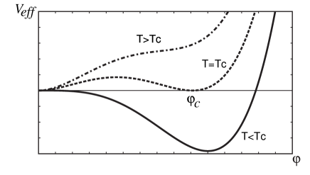
Figure 2: Qualitative form of the effective potential at several temperatures. The potential at $\varphi=0$ is normalized to be zero for all temperatures.

The first attempt to evaluate the effective potential was based on the loop expansion in finite-temperature field theory[34, 35, 36]. The effective potential in the minimal standard model (MSM), at the one-loop level, is given by

$$V_{\rm eff}(\varphi;T)=V_{\rm tree}(\varphi)+V^{(1)}(\varphi;T),$$ (4.2)

where $V_{\rm tree}(\varphi)$ is the tree-level potential,

$$V_{\rm tree}(\varphi)=-{1\over 2}\mu_{0}^{2}\varphi^{2}+{{\lambda_{0}}\over 4}\varphi^{4},$$ (4.3)

$V^{(1)}(\varphi;T)$ is the one-loop contribution

$$V^{(1)}(\varphi;T)=-{i\over 2}\sum_{A}c_{A}\int_{k}\log\det\left[i{\cal D}_{A}^{-1}(k;\varphi)\right]$$ (4.4)

and the order parameter $\varphi$ is introduced as the expectation value of the Higgs field as

$$\langle\Phi(x)\rangle={1\over{\sqrt{2}}}\pmatrix{0\cr\varphi\cr}.$$ (4.5)

Here $\mu_{0}^{2}$ and $\lambda_{0}$ are the bare parameters, which will be determined once one prescribes the renormalization. In(4.4), the subscript $A$ runs over all the species including the Faddeev-Popov ghosts, $c_{A}$ denotes the degrees of freedom of each particle and its statistics, that is, $c_{A}>0$ for bosons and $c_{A}<0$ for fermions, and ${\cal D}^{-1}$ is the inverse propagator, which is in general a matrix with Lorentz and internal symmetry indices and depends on $\varphi$ through its mass. The integration over the momentum should be understood as

$$\int_{k}\equiv iT\!\sum_{n=-\infty}^{\infty}\int{{d^{3}{\mib k}}\over{(2\pi)^{3}}}\qquad\mbox{with }k^{0}=\omega_{n}=\left\{\begin{array}[]{ll}2n\pi T&\mbox{ for bosons},\\ (2n+1)\pi T&\mbox{ for fermions}.\end{array}\right.$$ (4.6)

For example, $c_{W}=2$ and $i{{\cal D}^{-1}}_{W}^{\mu\nu}(k;\varphi)=(-k^{2}+m_{W}^{2}(\varphi))\eta^{\mu\nu}+(1-\xi^{-1})k^{\mu}k^{\nu}$ for $W$ boson in the $R_{\xi}$-gauge, where $m_{W}(\varphi)={1\over 2}g\varphi$, $c_{f}=-2$ and $i{\cal D}_{f}^{-1}(k;\varphi)=k\kern-5.50003pt\raise 0.60277pt\hbox{/}-m_{f}(\varphi)$ for a Dirac fermion with $m_{f}(\varphi)=y_{f}\varphi/\sqrt{2}$. The divergences in (4.4) are absorbed in the bare parameters by the renormalization at zero temperature. For the Higgs boson, $m^{2}_{H}(\varphi)=3\lambda\varphi^{2}-\mu^{2}$, so that $V^{(1)}(\varphi;T)$ becomes complex for small $\varphi$[35].  Since the free energy is originally a real quantity, this pathology will be caused by the loop expansion, which is invalid for small $\varphi$, and is expected to be cured if one takes the higher order contributions into account. At this point, we neglect the contributions from the Higgs and higher orders and discuss the structure of $V_{\rm eff}(\varphi;T)$. Now we consider only $W$ and $Z$ bosons and top quarks, since the contributions from the other fermions are negligible. Then the one-loop effective potential is

$$V_{\rm eff}(\varphi;T)=V_{0}(\varphi)+{\bar{V}}(\varphi;T),$$ (4.7)

where

$$V_{0}(\varphi) = -{1\over 2}\mu^{2}\varphi^{2}+{\lambda\over 4}\varphi^{4}+2Bv_{0}^{2}\varphi^{2}+B\varphi^{4}\left[\log\left({{\varphi^{2}}\over{v_{0}^{2}}}\right)-{3\over 2}\right],$$ (4.8)

$${\bar{V}}(\varphi;T) = {{T^{4}}\over{2\pi^{2}}}\left[6I_{B}(a_{W})+3I_{B}(a_{Z})-6I_{F}(a_{t})\right].$$ (4.9)

Here we follow the renormalization convention of Ref. [37], and

$$B = {3\over{64\pi^{2}v_{0}^{4}}}(2m_{W}^{4}+m_{Z}^{4}-4m_{t}^{4}),$$ (4.10)

$$I_{B,F}(a) = \int_{0}^{\infty}dx\,x^{2}\log\left(1\mp{e}^{-\sqrt{x^{2}+a^{2}}}\right),$$ (4.11)

where $v_{0}=246\mbox{GeV}$ is the minimum of $V_{0}(\varphi)$ and $a_{A}=m_{A}(\varphi)/T$.

For high temperatures $T>m_{W},m_{Z},m_{t}$, the integrals $I_{B,F}$ can be approximated by the high-temperature expansion[35]:

$$V_{\rm eff}(\varphi;T)\simeq D(T^{2}-T_{0}^{2})\varphi^{2}-ET\varphi^{3}+{{\lambda_{T}}\over 4}\varphi^{4},$$ (4.12)

where

$$D = {1\over{8v_{0}^{2}}}(2m_{W}^{2}+m_{Z}^{2}+2m_{t}^{2}),$$ (4.13)

$$E = {1\over{4\pi v_{0}^{3}}}(2m_{W}^{3}+m_{Z}^{3})\sim 10^{-2},$$ (4.14)

$$T_{0}^{2} = {1\over{2D}}(\mu^{2}-4Bv_{0}^{2}),$$ (4.15)

$$\lambda_{T} = \lambda-{3\over{16\pi^{2}v_{0}^{4}}}\left(2m_{W}^{4}\log{{m_{W}^{2}}\over{\alpha_{B}T^{2}}}+m_{Z}^{4}\log{{m_{Z}^{2}}\over{\alpha_{B}T^{2}}}\right.$$ (4.16)

$$\qquad\qquad\qquad\left.-4m_{t}^{4}\log{{m_{t}^{2}}\over{\alpha_{F}T^{2}}}\right)$$

with $\log\alpha_{B}=2\log\,4\pi-2\gamma_{E}$, $\log\alpha_{F}=2\log\,\pi-2\gamma_{E}$ and $\gamma_{E}=0.5772\cdots$ being the Euler constant. The effective potentials of other models which exhibit first-order phase transition will have a form similar to that of (4.12) with $E>0$, while each coefficient will be modified appropriately. By use of this approximate form, we see that at $T=T_{C}$, where the transition temperature $T_{C}$ is determined by

$$T_{C}^{2}={{T_{0}^{2}}\over{1-E^{2}/(\lambda_{T_{C}}D)}},$$ (4.17)

the effective potential has two degenerate minima at $\varphi=0$ and

$$\varphi_{C}={{2ET_{C}}\over{\lambda_{T_{C}}}}.$$ (4.18)

The presence of the $\varphi^{3}$-term with positive $E$ in the effective potential is essential for the EWPT to be first order. It originates from the zero-frequency mode of the bosons in the finite-temperature Feynman integral in (4.9). This can be seen as follows[37]. The zero-frequency contribution to $dV_{\rm eff}/d\varphi$ has the form of

$${{dV_{\rm eff}(\varphi;T)}\over{d\varphi}}\sim{{dm^{2}(\varphi)}\over{d\varphi}}\int{{d^{3}{\mib k}}\over{(2\pi)^{3}}}{1\over{{\mib k}^{2}+m^{2}(\varphi)}}=-{1\over{4\pi}}{{dm^{2}(\varphi)}\over{d\varphi}}\sqrt{m^{2}(\varphi)},$$ (4.19)

where the divergence which is absorbed by renormalization is dropped. Since this is proportional to $\varphi^{2}$, $V_{\rm eff}$ contains a $\varphi^{3}$-term upon integration. Note that within this approximation, the EWPT appears to be first order, since $V_{\rm eff}$ always has a $\varphi^{3}$-term whose coefficient has the correct sign.

Once the expectation value of the Higgs at $T_{C}$ is known, one can evaluate the sphaleron rate at $T_{C}$. Requiring that the sphaleron process decouples in the broken phase just after the EWPT imposes an upper bound on the Higgs mass[38]. This amounts to the condition that the sphaleron rate in the broken phase (3.7) multiplied by particle density $\sim T^{3}$ is smaller than the Hubble parameter (3.9), which yields

$${{\varphi_{C}}\over{T_{C}}}\mathrel{\hbox{\raise 0.86108pt\hbox{$>$}\kern-7.5pt\raise-3.87495pt\hbox{$\sim$}}}1.$$ (4.20)

This is converted to an upper bound on $\lambda$. Since the Higgs mass is given by $m_{H}={\sqrt{2}\lambda}v_{0}$ at the tree level, $m_{H}$ is bounded as

$$m_{H}\mathrel{\hbox{\raise 0.86108pt\hbox{$<$}\kern-7.5pt\raise-3.87495pt\hbox{$\sim$}}}46\mbox{GeV}.$$ (4.21)

This is obviously inconsistent with the present lower bound $m_{H}>58.4\mbox{GeV}$[2]. Although this upper bound may be a crude value, the decoupling of sphaleron process in general will require the Higgs be lighter than some bound. This upper bound will be relaxed if one extends the model to include extra bosons, which effectively enhance the $\varphi^{3}$-term.

Among these extended models are those with two Higgs doublets, including the minimal supersymmetric standard model (MSSM). We studied the massless two-Higgs-doublet model, in which the gauge symmetry is broken by the Coleman-Weinberg mechanism, without recourse to the high-temperature expansion. Our result shows that for the entire range of the parameters we considered, the EWPT is first order, the sphaleron decoupling condition is satisfied and the lightest Higgs scalar is as heavy as $63\mbox{GeV}$[39]. The more general two-Higgs-doublet model was studied by randomly scanning the vast parameter space[40]. For the parameters consistent with present experiments and allowing perturbation, the lightest Higgs scalar has mass $45\mathrel{\hbox{\raise 0.86108pt\hbox{$<$}\kern-7.5pt\raise-3.87495pt\hbox{$\sim$}}}m_{h}\mathrel{\hbox{\raise 0.86108pt\hbox{$<$}\kern-7.5pt\raise-3.87495pt\hbox{$\sim$}}}190\mbox{GeV}$. The upper bound on the Higgs mass in the MSSM was evaluated for various values of the soft supersymmetry-breaking parameters and was found to be near the experimental lower bound[41].  We note that all these results are based on the one-loop effective potential and the latter two works used the high-temperature expansion. In general, for these extended models, we have more chances to satisfy the bound on the Higgs mass consistent with experiments and to obtain first-order EWPT.

Here we shall comment on higher-order studies of the effective potential. The most dominant contributions are the daisy type diagrams, and summing up these gives a well-defined effective potential[35]. Since these diagrams correspond to infinite-order mass corrections, some authors evaluate the ‘improved’ effective potential simply by replacing $m^{2}$ of the particle in the loop with $m^{2}+\Pi(\varphi)$ in the one-loop effective potential, where $\Pi(\varphi)$ is the one-loop polarization. Although this prescription may somehow cure the pathology of complex effective potential for smaller $\varphi$, it does not yield correct answer[37].  The correct method gives a smaller value of $E$ in (4.12), which means a weaker first-order phase transition. Some two-loop calculations suggest the opposite situation. The two-loop corrections to the ring-improved one-loop effective potential were found to raise the lower bound derived from the sphaleron decoupling condition, while it still rules out the MSM[42]. The two-loop effective potential was shown to increase the strength of the first-order EWPT[44]. These two-loop corrections are so large that we still need more reliable evaluation for a definitive conclusion.

Besides these analytic investigations, the static properties of the EWPT have been studied numerically by the lattice simulations[45]. Since at present the electroweak theory cannot be put on the lattice completely, its subsystem, $SU(2)$ gauge-Higgs system with one Higgs doublet, has been taken, and two methods have been applied to the simulation. At high temperatures, fermions attain effective masses of $O(T)$ because of their antiperiodicity along the imaginary time direction, even if they are massless at zero temperature. This fact might justify this approximation neglecting all the fermions in the model at high temperatures. One of the simulations is the standard one on the periodic euclidean four-dimensional lattice. The other is that of the effective three-dimensional theory, which is obtained by taking the high-temperature limit. In this limit, the euclidean time period, $1/T$, is smaller and the system is reduced to that of the fields, which are zero modes of the Matsubara frequency in the original system. That is, the effective three-dimensional system is composed of an $SU(2)$ gauge field with one Higgs doublet and one Higgs triplet, which is the remnant of the time-component of the original gauge field. Correspondingly, the parameters come to have temperature-dependence, which are determined by evaluating finite temperature Green’s functions in both the original and the reduced theory and by matching them[46]. Because of Elitzur’s theorem, no local symmetry is broken on the lattice, so that $\langle\phi\rangle=0$[47]. The measured quantities are expectation values of the gauge invariant operators such as $\langle\phi^{\dagger}\phi\rangle$, its jump, transition temperature $T_{C}$, latent heat and surface tension. The latent heat is obtained by the derivative with respect to temperature of the difference of the free energy between the two phases, just as the continuum theory. There are three methods to measure the surface tension between the two phases. As for the comparison of the results of these simulations with the continuum analysis, see Ref. [48]. According to Ref. [48], the numerical results coincide with those of the continuum two-loop perturbation theory, up to the Higgs masses of about $70\mbox{GeV}$. For example, the three-dimensional reduced theory gives, with both perturbative and numerical methods, $T_{C}\simeq 93\mbox{GeV}$ and $\varphi_{C}/T_{C}\simeq 1.8$ for $m_{H}=35\mbox{GeV}$, $T_{C}\simeq 140\mbox{GeV}$ and $\varphi_{C}/T_{C}\simeq 0.7$ for $m_{H}=60\mbox{GeV}$, $T_{C}\simeq 155\mbox{GeV}$ and $\varphi_{C}/T_{C}\simeq 0.6$ for $m_{H}=70\mbox{GeV}$. It also yields the result that if we denote the surface tension by $\sigma$, $\sigma/T_{C}^{3}\simeq 0.84$ for $m_{H}=18\mbox{GeV}$, $\sigma/T_{C}^{3}\simeq 0.065$ for $m_{H}=35\mbox{GeV}$ and $\sigma/T_{C}^{3}\simeq 0.008$ for $m_{H}=49\mbox{GeV}$ by the four-dimensional simulation. From these results, the EWPT of the MSM is first order for $m_{H}\mathrel{\hbox{\raise 0.86108pt\hbox{$<$}\kern-7.5pt\raise-3.87495pt\hbox{$\sim$}}}70\mbox{GeV}$. The strength of the transition rapidly decreases as $m_{H}$ increases. For $m_{H}\geq 60\mbox{GeV}$, (4.20) is not satisfied, but the upper bound on $m_{H}$ might be weakened since temperature in the broken phase is lower than $T_{C}$ because of supercooling.

These quantities compared between analytic and numerical methods are those derived from the effective potential but not itself. One can, in principle, calculate the effective potential by numerical methods, but its form is always convex[36] so that it does not give quantities such as the height and width of the barrier of the effective potential dividing the two phases. Our aim is to obtain a ‘classical’ effective potential which offers information about the first-order phase transition. Such an effective potential should reproduce the results of the lattice simulations and have a shape like Fig. 2.

As we shall see in the next section, to have an efficient $CP$ violation, extension of the Higgs sector would be needed. Further, such extension would open the chance to fulfill the condition (4.20) within the present Higgs mass bound. Hence both analytic and numerical studies of such models would be desired.

4.2 Dynamics of the phase transition

To have nonzero BAU, we need a nonequilibrium state, which is realized by expanding bubbles created at the first-order EWPT. Whether the EWPT is a first-order transition accompanying nucleation and consecutive growth of bubbles of the broken phase in the symmetric phase will be determined by the form of the effective potential. If the EWPT proceeds with bubble nucleation and growth, the width and velocity of the bubble wall are essential to evaluate the baryon number generated. The nucleation rate of the bubbles is also crucial, since if their nucleation dominates over their growth, the total region which experiences nonequilibrium conditions will decrease.

A crude picture of how the EWPT proceeds can be gained as follows. Suppose that the effective potential at temperatures around $T_{C}$ is known. The nucleation rate per unit time and volume is given by[26]

$$I(T)=I_{0}{e}^{-\Delta F(T)/T},$$ (4.22)

where the prefactor $I_{0}$ is determined by temperature, viscosity and correlation length in the symmetric phase and $\Delta F$ is the change in the free energy caused by formation of a bubble. As long as the thin-wall approximation is valid, $\Delta F$ is approximately given by

$$\Delta F(T)={{4\pi}\over 3}r^{3}[p_{s}(T)-p_{b}(T)]+4\pi r^{2}\sigma,$$ (4.23)

where $p_{s(b)}$ is the pressure in the symmetric (broken) phase and is given by

$$p_{s}(T)=-V_{\rm eff}(0;T),\qquad p_{b}(T)=-V_{\rm eff}(\varphi(T);T).$$ (4.24)

In general, $p_{s}(T)<p_{b}(T)$ because of supercooling. $\sigma$ is the surface energy density given by $\sigma\simeq\int dz(d\varphi/dz)^{2}$, with $z$ being the coordinate perpendicular to the bubble wall. For smaller radius $r$, the second term on the right-hand side of (4.23) dominates so that the surface tension shrinks the bubbles. For larger $r$, the first term dominates and the bubble expands to lower the free energy. The critical bubble has a boundary radius between these bubbles, whose radius is

$$r_{*}(T)={{2\sigma}\over{p_{b}(T)-p_{s}(T)}}.$$ (4.25)

With the free energy $V_{\rm eff}(\varphi;T)$ known, one can calculate various thermodynamical quantities. For example, the entropy density is given by $s=-{\partial}V_{\rm eff}/{\partial}T$ and the energy density is $\rho=V_{\rm eff}-Ts$. The latent heat is the difference of the energy density between the two phases. How the phase transition proceeds may be characterized by the fraction of space which has been converted to the broken phase, $f(t)$. It obeys the integral equation

$$f(t)=\int_{t_{C}}^{t}dt^{\prime}\,I(T(t^{\prime}))[1-f(t^{\prime})]V(t^{\prime},t),$$ (4.26)

where $V(t^{\prime},t)$ is the volume of a bubble at $t$ which was nucleated at $t^{\prime}<t$. Here, the time $t$ and temperature $T$ are related by the scale factor of the universe $R$ at $t$, since $\rho\propto R^{-4}$ for the radiation-dominated universe and $\rho=(\pi^{2}/30)g_{*}T^{4}$. (See Appendix A.) $V(t^{\prime},t)$ is taken as

$$V(t^{\prime},t)={{4\pi}\over 3}\left[r_{*}(T(t^{\prime}))+\int_{t^{\prime}}^{t}dt^{\prime\prime}\,v(T(t^{\prime\prime}))\right]^{3},$$ (4.27)

where $v(T)$ is the wall velocity. This simple approach does not take into account interactions and fluctuations of the bubbles. The wall velocity and thickness are estimated by solving dynamical equation for $\varphi(x)$ with friction[49, 50]. In Ref.[51], (4.26) is numerically analyzed by use of the wall velocity given in Ref.[49] with the one-loop improved effective potential of the MSM for $m_{H}=60\mbox{GeV}$ and $m_{t}=120\mbox{GeV}$. The results show that if we measure the time after the temperature reached $T_{C}$, (1) at $6.5\times 10^{-14}\mbox{sec}$, bubbles began to nucleate, (2) at $6.87\times 10^{-14}\mbox{sec}$, the nucleation was turned off and then only about $10\%$ of the universe had been converted to the broken phase, then (3) the remaining $90\%$ of the universe is converted by the bubble growth with almost constant velocity of about $0.8$, and (4) the transition is completed at $7.05\times 10^{-14}\mbox{sec}$. Further if we denote the temperature at which the bubble nucleation begins by $T_{N}$, $(T_{C}-T_{N})/T_{C}\simeq 2.5\times 10^{-4}$, which means the EWPT shows small supercooling.

All these results are based on the effective potential of the MSM at the one-loop level or the improved version of it. As mentioned, the above estimation neglects the interactions of the bubbles and various fluctuations. For weak first-order transitions, thermal fluctuations might affect the dynamics of the transition. Then the barrier dividing the symmetric and broken phases of $V_{\rm eff}$ is so low that the two phases may be mixed by thermal fluctuations. In such a case, the EWPT might proceed not with nucleation of the critical bubbles but with that of the subcritical bubbles[52]  so that the simple analysis above may no longer be valid.

The numerical simulations as well as the two-loop effective potential suggest a stronger first-order transition in the MSM than the one-loop result. Extensions of the standard model with more Higgs scalars may also lead to a stronger transition, since the upper bound on the Higgs mass is raised somehow and since this also implies that $\varphi_{C}$ is larger for a given Higgs mass. In fact, our work on the two-Higgs-doublet model supports this fact and thinner bubble walls[39].

5 Mechanism of the electroweak baryogenesis

If the sphaleron process is in equilibrium in the symmetric phase and decouples in the broken phase at the EWPT, it is out of equilibrium around the moving bubble wall dividing the two phases. In this section, we review how the baryon number is generated by use of this nonequilibrium situation. Around the expanding bubble wall, the expectation value of the Higgs field is schematically depicted in Fig. 3, where $\varphi$ represents the absolute value of the Higgs scalar. $v_{0}$ is that in the broken phase and $v_{co}$ is the value above which the sphaleron process decouples.

Figure 3: Profile of the expanding bubble wall. In the region right to the vertical dashed line, the sphaleron process is effective. $v_{w}$ is the wall velocity.

There are two mechanisms of the electroweak baryogenesis; classical or adiabatic mechanism, which is called ‘spontaneous baryogenesis’ and quantum mechanical one, which is also called ‘charge transport scenario’. Although these two mechanisms may be responsible for baryogenesis at the same time, the former is effective for a thick bubble wall while the latter is effective for a thin wall, as we shall see below. Further both require extensions of the Higgs sector in the MSM, except for the scenario proposed by Farrar and Shaposhnikov[53]. The spontaneous scenario was proposed earlier than the charge transport mechanism. It, however, was pointed out that it would generate too small a number of baryons in its original form. After the charge transport scenario was proposed, the classical mechanism was revived by introducing a nonlocal effect, which is an advantage of the charge transport scenario.

5.1 Charge transport scenario

Fermions interact with the bubble wall through the Yukawa couplings, which in general contain $CP$ violation. If the $CP$ violation is not constant over spacetime, it cannot be rotated out by a biunitary transformation so that there remains a physical effect. This $CP$ violation discriminates between the interaction of the fermions and that of the antifermions with the bubble wall. That is, the reflection rate of the fermions does not coincide with that of antifermions so that the net current of some quantum number flows into the symmetric phase region, where the sphaleron process is effective. There the previous equilibrium state will be forced to shift to new state, which will contain baryon number excess. One can see how this occurs by solving the kinetic equations, which will contain various interactions of different time scales. Such equations are in general difficult to solve. When the bubble wall moves with constant velocity, the flux will bias the free energy along the baryon number to realize a stationary nonequilibrium state, as depicted in Fig. 4.

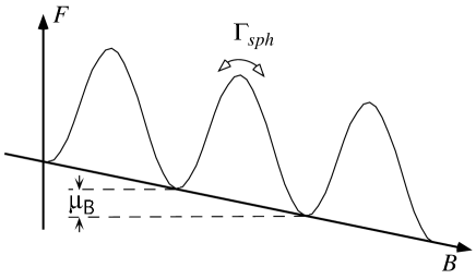
Figure 4: The free energy as a function of the baryon number is biased and a nonequilibrium stationary state is realized.

In this case, the constant flow of the flux will induce a nonzero chemical potential for the baryon number. Then the steady state produces the baryon number according to the equation

$${\dot{n}}_{B}\simeq-{{\mu_{B}\Gamma_{\rm sph}}\over T},$$ (5.1)

where $\Gamma_{\rm sph}$ is the sphaleron rate in the symmetric phase (3.8). For the derivation of this equation, see Appendix B.

Cohen, Kaplan and Nelson related the flux flowing into the symmetric phase to the generated baryon number as follows[54]. Suppose that a left(right)-handed fermion of species $i$ with charge $Q_{L(R)}^{i}$ is incident from the symmetric phase region. The expectation value of the injected charge in the symmetric phase, which has been brought by the reflection and transmission of the fermions, is given by

$$\Delta Q_{i}^{s} = [(Q_{R}^{i}-Q_{L}^{i})R^{s}_{L\rightarrow R}+(-Q_{L}^{i}+Q_{R}^{i}){\bar{R}}^{s}_{L\rightarrow R}$$ (5.2)

$$+(-Q_{L}^{i})(T^{s}_{L\rightarrow L}+T^{s}_{L\rightarrow R})-(-Q_{R}^{i})({\bar{T}}^{s}_{R\rightarrow L}+{\bar{T}}^{s}_{R\rightarrow R})]f^{s}_{Li}$$

$$+[(Q_{L}^{i}-Q_{R}^{i})R^{s}_{R\rightarrow L}+(-Q_{R}^{i}+Q_{L}^{i}){\bar{R}}^{s}_{L\rightarrow R}$$

$$+(-Q_{R}^{i})(T^{s}_{R\rightarrow L}+T^{s}_{R\rightarrow R})-(-Q_{L}^{i})({\bar{T}}^{s}_{L\rightarrow L}+{\bar{T}}^{s}_{L\rightarrow R})]f^{s}_{Ri},$$

where $R^{s}_{R\rightarrow L}$ (${\bar{R}}^{s}_{R\rightarrow L}$) is the reflection coefficient for the right-handed fermion (antifermion) incident from the symmetric phase region and reflected as the left-handed one, $T$’s are the transmission coefficients and $f^{s}_{L(R)}$ is the left(right)-handed fermion flux density in the symmetric phase, which will be given below. Here we have used ${\bar{f}}^{s}_{L}=f^{s}_{R}$. In a similar manner, the expectation value of the change of the charge brought by the transmission of the fermions incident from the broken phase region is

$$\Delta Q_{i}^{b} = Q_{L}^{i}(T^{b}_{L\rightarrow L}f^{b}_{Li}+T^{b}_{R\rightarrow L}f^{b}_{Ri})+Q_{R}^{i}(T^{b}_{L\rightarrow R}f^{b}_{Li}+T^{b}_{R\rightarrow R}f^{b}_{Ri})$$

$$+(-Q_{L}^{i})({\bar{T}}^{b}_{R\rightarrow L}f^{b}_{Li}+{\bar{T}}^{b}_{L\rightarrow L}f^{b}_{Ri})+(-Q_{R}^{i})({\bar{T}}^{b}_{R\rightarrow R}f^{b}_{Li}+{\bar{T}}^{b}_{L\rightarrow R}f^{b}_{Ri}).$$

By use of the unitarity

$$R^{s}_{L\rightarrow R}+T^{s}_{L\rightarrow L}+T^{s}_{L\rightarrow R}=1,\qquad\mbox{etc.}$$ (5.4)

and the reciprocity[55]

$$T^{s}_{R\rightarrow L}+T^{s}_{R\rightarrow R}=T^{b}_{L\rightarrow L}+T^{b}_{R\rightarrow L},\qquad\mbox{etc.}$$ (5.5)

the total expectation value of the change is

$$\Delta Q^{s}_{i}+\Delta Q^{b}_{i}=(Q_{L}^{i}-Q_{R}^{i})(f^{s}_{i}-f^{b}_{i})\Delta R,$$ (5.6)

where

$$\Delta R\equiv R^{s}_{R\rightarrow L}-{\bar{R}}^{s}_{R\rightarrow L},$$ (5.7)

and we have put $f^{s(b)}_{iL}=f^{s(b)}_{iR}\equiv f^{s(b)}_{i}$. The total charge injected into the symmetric phase can be obtained by integrating this in the rest frame of the bubble wall and going back to the rest frame of the medium,

$$F^{i}_{Q}={{Q_{L}^{i}-Q_{R}^{i}}\over{4\pi^{2}\gamma}}\int_{m_{0}}^{\infty}dp_{L}\int_{0}^{\infty}dp_{T}\,p_{T}\left[f_{i}^{s}(p_{L},p_{T})-f_{i}^{b}(-p_{L},p_{T})\right]\Delta R({{m_{0}}\over a},{{p_{L}}\over a}).$$ (5.8)

Here

$$f_{i}^{s}(p_{L},p_{T}) = {{p_{L}}\over E}{1\over{\exp[\gamma(E-v_{w}p_{L})/T]+1}},$$

$$f_{i}^{b}(-p_{L},p_{T}) = {{p_{L}}\over E}{1\over{\exp[\gamma(E+v_{w}\sqrt{p_{L}^{2}-m_{0}^{2}})/T]+1}},$$ (5.9)

are the fermion flux densities in the symmetric and broken phase, respectively, $m_{0}$ is the fermion mass in the broken phase, $v_{w}$ is the wall velocity, $\gamma=1/\sqrt{1-v_{w}^{2}}$, $E=\sqrt{p_{L}^{2}+p_{T}^{2}}$, $p_{T}$ being the transverse momentum with respect to the bubble wall. If we calculate $\Delta R$ with zero-temperature Dirac equation in the presence of the $CP$-violating potential, it is a function of $m_{0}/a$ and $p_{L}/a$, where $a^{-1}$ is the wall width.

$\Delta R$ contains the information of $CP$ violation for the model with which we are concerned. In the MSM, $CP$ violation enters only through the Kobayashi-Maskawa (KM) matrix in the charged-current interactions. Farrar and Shaposhnikov proposed that even in the MSM, the interactions of the quarks with the plasma of the gauge bosons and Higgs bosons, which modify the dispersion relations of the quasiparticles, may yield significant baryon number[53]. The effect of the KM matrix comes into the dispersion relations of $O(\alpha_{W})$ and there are claims that QCD damping effects, whose scale is shorter than that of other interactions, may bring quantum decoherence[56]. Hence to obtain enough BAU only via electroweak baryogenesis, we would have to employ an extra source of $CP$ violation, such as that in the Higgs sector in the two-Higgs-double model. The $CP$ violation in the Higgs sector affects the fermion propagation around the bubble wall at the tree level, so it was the first model considered in the charge transport scenario[54]. As for the quantum number injected in the symmetric phase, we must take that conserved there and satisfying $Q_{L}-Q_{R}\not=0$. One such charge is the weak hypercharge $Y$. Now let us see how the injected hypercharge biases baryon number.

As we stated above, the change of state caused by the injection of hypercharge would be described by the kinetic equations. Here we assume that the bubble wall is macroscopic and moves with almost constant velocity, and that the state shifts to a new steady state. Such a situation would be described by the chemical potentials for all the particles in equilibrium. This simple picture would be valid in the region far from the wall and in the case that the elementary processes are fast enough to realize a new stationary state. For simplicity, we consider only the third generation and the case that all the particles had been in equilibrium with $n_{B}=n_{L}=0$ through the gauge and Yukawa interactions before the injection of the hypercharge. Now we introduce the chemical potentials

$$\mu_{t_{L}},\mu_{b_{L}},\mu_{t_{R}},\mu_{b_{R}},\mu_{\tau_{L}},\mu_{\nu_{\tau}},\mu_{\tau_{R}},\mu_{W}\mbox{ for $W^{-}$},\mu_{0}\mbox{ for $\phi^{0}$},\mu_{-}\mbox{ for $\phi_{-}$}.$$

When the charged-current interaction is in chemical equilibrium,

$$\mu_{W}=\mu_{0}+\mu_{-}=-\mu_{t_{L}}+\mu_{b_{L}}=-\mu_{\nu_{\tau}}+\mu_{\tau_{L}},$$ (5.10)

and when the Yukawa interaction is in chemical equilibrium,

$$\mu_{0}=-\mu_{t_{L}}+\mu_{t_{R}}=-\mu_{b_{L}}+\mu_{b_{R}}=-\mu_{\tau_{L}}+\mu_{\tau_{R}}.$$ (5.11)

No further new equations are derived if the other elementary processes are in equilibrium. We also introduce the chemical potentials for quantum numbers which are conserved or almost conserved because of the slow processes:

$$\mu_{B-L},\quad\mu_{Y},\quad\mu_{I_{3}};\quad\mu_{B}.$$

Here we assume that the sphaleron process is out of equilibrium. Otherwise, $\mu_{B}$ vanishes so that the baryon number is not generated. The chemical potentials of the particles are expressed by these as

$$\mu_{t_{L}(b_{L})} = {1\over 3}\mu_{B}+{1\over 3}\mu_{B-L}+{1\over 6}\mu_{Y}+(-){1\over 2}\mu_{I_{3}},$$

$$\mu_{t_{R}} = {1\over 3}\mu_{B}+{1\over 3}\mu_{B-L}+{2\over 3}\mu_{Y},$$

$$\mu_{b_{R}} = {1\over 3}\mu_{B}+{1\over 3}\mu_{B-L}-{1\over 3}\mu_{Y},$$

$$\mu_{\tau_{L}(\nu_{\tau})} = -\mu_{B-L}-{1\over 2}\mu_{Y}+(-){1\over 2}\mu_{I_{3}},$$

$$\mu_{0(-)} = +(-){1\over 2}\mu_{Y}-{1\over 2}\mu_{I_{3}},$$

$$\mu_{W} = -\mu_{I_{3}}.$$ (5.12)

Because of (3.11), the baryon and lepton number densities are given by

$$n_{B} = 3\cdot{{T^{2}}\over 6}(\mu_{t_{L}}+\mu_{t_{R}}+\mu_{b_{L}}+\mu_{b_{R}})={{T^{2}}\over 3}(2\mu_{B}+2\mu_{B-L}+\mu_{Y}),$$ (5.13)

$$n_{L} = {{T^{2}}\over 6}(\mu_{\nu_{\tau}}+\mu_{\tau_{L}}+\mu_{\tau_{R}})={{T^{2}}\over 6}(-3\mu_{B-L}-2\mu_{Y}).$$ (5.14)

If $n_{B}=n_{L}=0$ before the injection of the hypercharge flux,

$$\mu_{B-L}=-{2\over 3}\mu_{Y},\qquad\mu_{B}={1\over 6}\mu_{Y},$$ (5.15)

hold because of (5.13) and (5.14). Then the hypercharge density, which is expressed by the chemical potentials of the particles, can be given, with the help of (5.12) and (5.15), by

$${Y\over 2} = {{T^{2}}\over 6}\left\{3\left[{1\over 6}(\mu_{t_{L}}+\mu_{b_{L}})+{2\over 3}\mu_{t_{R}}-{1\over 3}\mu_{b_{R}})\right]-{1\over 2}(\mu_{\nu_{\tau}}+\mu_{\tau_{L}})-\mu_{\tau_{R}}\right\}$$ (5.16)

$$\qquad+{{T^{2}}\over 3}{1\over 2}(\mu_{0}-\mu_{-})m$$

$$= {{T^{2}}\over 6}(m+{5\over 3})\mu_{Y},$$

where $m$ is the number of the Higgs doublets. From (5.15) and (5.16), we have

$$\mu_{B}={Y\over{2(m+5/3)T^{2}}}.$$ (5.17)

Thus the injected hypercharge biases the free energy along the direction of the baryon number. By use of (5.1), we have the generated baryon number density

$$n_{B}=-{{\Gamma_{\rm sph}}\over T}\int dt\,\mu_{B}=-{{\Gamma_{\rm sph}}\over{2(m+5/3)T^{3}}}\int dt\,Y.$$ (5.18)

If we denote the hypercharge density at distance $z$ from the bubble wall by $\rho_{Y}(z)$, the integral of $Y$ is estimated as

$$\int dt\,Y=\int_{-\infty}^{z/v_{w}}dt\,\rho_{Y}(z-v_{w}t)={1\over{v_{w}}}\int_{0}^{\infty}dz\,\rho_{Y}(z).$$ (5.19)

Since the hypercharge supplied from the wall would reach a finite distance when it is caught up with the wall, the last integral above will be approximated as

$${1\over{v_{w}}}\int_{0}^{\infty}dz\,\rho_{Y}(z)\simeq{{F_{Y}\tau}\over{v_{w}}},$$ (5.20)

where $\tau$ is the transport time within which the scattered fermions are captured by the wall. Hence the generated baryon asymmetry is

$${{n_{B}}\over s}\simeq{\cal N}{{100}\over{\pi^{2}g_{*}}}\cdot\kappa\alpha_{W}^{4}\cdot{{F_{Y}}\over{v_{w}T^{3}}}\cdot\tau T,$$ (5.21)

where ${\cal N}$ is a model-dependent constant of $O(1)$. $\tau$ may be approximated by the mean free time or diffusion time $D/v_{w}$ with the diffusion constant $D$ of the charge carrier, where $D\simeq 1/T$ for quarks and $D\simeq(10^{2}\sim 10^{3})/T$ for leptons[57]. It was shown that if the forward scattering is enhanced, even for the top quark, $\tau T\simeq 10\sim 10^{3}$ depending on $v_{w}$, where the maximum value is realized at $v_{w}\simeq 1/\sqrt{3}$[54]. For this optimal case,

$${{n_{B}}\over s}\simeq 10^{-3}\cdot{{F_{Y}}\over{v_{w}T^{3}}}.$$ (5.22)

Then the hypercharge flux $F_{Y}/(v_{w}T^{3})\sim O(10^{-7})$ would be sufficient to explain the present BAU. For leptons, $\tau T$ is much larger than that of quarks, since its propagation is not disturbed by strong interactions. As we shall see below, the hypercharge flux depends not only on the mass of the carrier but also the wall width and velocity.

Now we evaluate the chiral charge flux in (5.8). Here we assume that the simple zero-temperature Dirac equation describes the propagation of fermions well. This is justified when the mean free path of the fermion is larger than the bubble wall width. Since the dynamics of the EWPT in the extended models is not well established, we treat the wall width and velocity as parameters and calculate the flux as a function of them. The problem is to solve the Dirac equation in the background of the bubble wall. The bubble wall is composed of classical gauge and Higgs fields. As we shall see in the next section, its profile will be composed of the Higgs scalar only and the gauge fields are pure-gauge type so that we fix the gauge such that the gauge fields vanish. Then the Dirac equation to be solved is, for one flavor,

$$i{\partial}\kern-5.50003pt\raise 0.60277pt\hbox{/}\psi(x)-m(x)P_{R}\psi(x)-m^{*}(x)P_{L}\psi(x)=0,$$ (5.23)

where $P_{R}={{1+\gamma_{5}}\over 2}$,$P_{L}={{1-\gamma_{5}}\over 2}$ and $m(x)=-f\langle\phi(x)\rangle$ is a complex-valued function of spacetime, with $f$ being the Yukawa coupling. When the radius of the bubble is macroscopic and the bubble is static or moving with a constant velocity, we can regard $m(x)$ as a static function of only one spatial coordinate:

$$m(x)=m(t,{\mib x})=m(z).$$

Putting

$$\psi(x)={e}^{i\sigma(-Et+{\mib p}_{T}\cdot{\mib x}_{T})},\qquad(\sigma=+1\mbox{ or }-1)$$ (5.24)

(5.23) is reduced to

$$\left[\sigma(\gamma^{0}E-\gamma_{T}p_{T})+i\gamma^{3}{\partial}_{z}-m_{R}(z)-i\gamma_{5}m_{I}(z)\right]\psi_{E}({\mib p}_{T},z)=0,$$ (5.25)

where

$${\mib p}_{T} = (p^{1},p^{2}),\qquad{\mib x}_{T}=(x^{1},x^{2}),\qquad p_{T}=\left|{\mib p}_{T}\right|,\qquad$$

$$\gamma_{T}p_{T} = \gamma^{1}p^{1}+\gamma^{2}p^{2},$$

$$m(z) = m_{R}(z)+im_{I}(z).$$

If we denote $E=E^{*}\cosh\eta$ and $p_{T}=E^{*}\sinh\eta$ with $E^{*}=\sqrt{E^{2}-p_{T}^{2}}$, ${\mib p}_{T}$ in (5.25) can be eliminated by the Lorentz transformation $\psi\mapsto\psi^{\prime}={e}^{-\eta\gamma^{0}\gamma_{5}}\psi$:

$${\partial}_{z}\psi_{E}(z)=i\gamma^{3}\left[-\sigma E^{*}\gamma^{0}+m_{R}(z)+i\gamma_{5}m_{I}(z)\right]\psi_{E}(z).$$ (5.26)

This equation was first solved numerically in a finite region containing the bubble wall[54],  with the following potential

$$m(z)=m_{0}{{1+\tanh(az)}\over 2}\exp\left(-i\pi{{1-\tanh(az)}\over 2}\right).$$ (5.27)

The nontrivial $z$-dependence of the phase of $m(z)$ yields $CP$ violation in the Dirac equation. If it were independent of $z$, the phase could be eliminated by redefinition of the wave functions, so that it would yield no physical effect. We analyzed (5.26) by the perturbative method[55],  which can be applied when the imaginary part of the mass function is much less than $m_{0}$, as well as by numerical methods[58],  which solves (5.26) in the infinite region and gives the results with any precision. In Fig. 5, we show data for $\Delta R$ with the potential (5.27), which were obtained numerically[58].

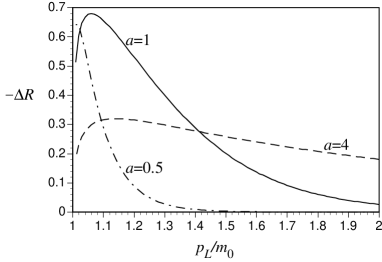
Figure 5: $\Delta R$ for the potential (5.27). We take $m_{0}=1$.

For higher incident energy, $\left|\Delta R\right|$ decreases exponentially. This is because for $p_{L}>m_{0}$, the wave function is obtained approximately by the WKB method, which infers that $R_{R\rightarrow L}$ and ${\bar{R}}_{R\rightarrow L}$ are exponentially small. $\left|\Delta R\right|$ can be $O(1)$ when the wall width is comparable to the Compton wave length of the carrier, i.e., $m_{0}/a\sim O(1)$. Note that larger Yukawa coupling does not always yield larger asymmetry in the reflection coefficients. The chiral charge flux, which is essential to determine the generated BAU, is evaluated by inserting $\Delta R$ into (5.8). We normalize it in a dimensionless form as

$${{F_{Q}}\over{uT^{3}(Q_{L}-Q_{R})}},$$ (5.28)

which enters in the baryon asymmetry of (5.21) or (5.22). The numerical results for the potential (5.27) are shown in Fig. 6, Fig. 7 and Fig. 8 for the wall velocities $v_{w}=0.1$, $v_{w}=1/\sqrt{3}\simeq 0.58$ and $v_{w}=0.98$, respectively, as functions of the carrier mass and the wall width. Here we take $T=100\mbox{GeV}$.

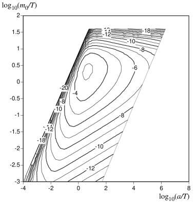
Figure 6: Contour plot of the chiral charge flux, normalized as $\log_{10}\left[-F_{Q}/(v_{w}T^{3}(Q_{L}-Q_{R}))\right]$ for the potential (5.27). Here we take $v_{w}=0.1$ and $T=100\mbox{GeV}$.

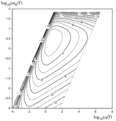
Figure 7: Contour plot of the chiral charge flux, normalized as $\log_{10}\left[-F_{Q}/(v_{w}T^{3}(Q_{L}-Q_{R}))\right]$ for the potential (5.27). Here we take $v_{w}=0.58$ and $T=100\mbox{GeV}$.

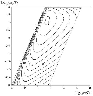
Figure 8: Contour plot of the chiral charge flux, normalized as $\log_{10}\left[-F_{Q}/(v_{w}T^{3}(Q_{L}-Q_{R}))\right]$ for the potential (5.27). Here we take $v_{w}=0.98$ and $T=100\mbox{GeV}$.

These figures suggest that the flux rapidly decreases for a heavier carrier and thicker wall and the region in which $-F_{Q}/(v_{w}T^{3}(Q_{L}-Q_{R}))>10^{-7}$ becomes broader for larger wall velocity. The maxima in these figures are realized at $a\sim T$, for which the wave length of the carrier is comparable to the wall thickness. For a thick bubble wall $a\simeq 40/T$, fermions of mass $0.1T<m_{0}<T$ can yield a flux larger than $10^{-7}$, while for a thin wall case $a\simeq 1/T$, fermions of mass $0.03T<m_{0}<10T$ can yield sufficient flux.

To calculate the flux, we assumed the form of the complex mass as (5.27). It yields no $CP$ violation in the broken phase so as to be free from any experimental limitations. However, the profile of the bubble wall should be determined dynamically. This is the subject of the next section, and it will also affect the other scenario of the electroweak baryogenesis.

5.2 Spontaneous baryogenesis

This scenario, in contrast to that in the previous subsection, is classical and effective for thick bubble walls. Although this scenario has several variants, the first proposed may be that by Shaposhnikov[38], That case depends on the existence of the condensation of the Chern-Simons number, which adds a $CP$-violating term in the effective action as

$$\Delta S_{\rm eff}=\mu N_{CS},$$ (5.29)

where $N_{CS}$ is defined by (3.4). This scenario fails in the MSM since it can induce at most $\mu=10^{-15}$ while $\mu=10^{-4}$ is needed to explain the BAU[38]. It is later elaborated by noting that in the two-Higgs-doublet extension of the MSM, the effective action takes the form as

$$\Delta{\cal L}_{\rm eff}=-{{g^{2}N_{f}}\over{24\pi^{2}}}\theta(x)F_{\mu\nu}(x){\tilde{F}}^{\mu\nu}(x),$$ (5.30)

where $\theta(x)$ is the relative phase of the two Higgs doublets[59], This term is $CP$-invariant since $\theta(x)$ is $CP$ odd, so that it is free from any constraint on $CP$ violation. A nontrivial evolution of $\theta(x)$ during the EWPT would induce asymmetry like $\mu$ in (5.29), upon integrated by parts. For high temperatures, the factor in front of the Chern-Simons number is accompanied by $(m_{t}/T)^{2}$ coming from the top quark loop[60]. Cohen et al. proposed a different approach, which utilizes the bias for the hypercharge in place of the Chern-Simons number, in the two-Higgs-doublet extension of the MSM[61], Their observation was that if the neutral component of the two Higgs scalar takes the form

$$\phi_{j}^{0}(x)=\rho_{j}(x){e}^{i\theta_{j}},\qquad(j=1,2)$$ (5.31)

where only $\phi_{1}$ is supposed to couple to the fermions, one can eliminate $\theta_{1}$ from the Yukawa coupling by an anomaly-free ($U(1)_{Y}$) rotation, which changes the fermion kinetic terms by

$$2{\partial}_{\mu}\theta_{1}(x)\left[{1\over 6}{\bar{q}}_{L}(x)\gamma^{\mu}q_{L}(x)+{2\over 3}{\bar{u}}_{R}(x)\gamma^{\mu}u_{R}(x)-{1\over 3}{\bar{d}}_{R}(x)\gamma^{\mu}d_{R}(x)\right.$$

$$\qquad\qquad\qquad\left.-{1\over 2}{\bar{l}}_{L}(x)\gamma^{\mu}l_{L}(x)-{\bar{e}}_{R}(x)\gamma^{\mu}e_{R}(x)\right],$$ (5.32)

where summation over generation is implicit. During the EWPT, $\theta_{1}(x)$ will behave nontrivially so that $\langle\dot{\theta}_{1}\rangle\not=0$. Then $\langle\dot{\theta}_{1}\rangle$ will play the role of ‘charge potential’. If this biases the hypercharge in the symmetric phase region, the same procedure to generate the baryon number as discussed in the charge transport scenario works here. They estimated the generated baryon asymmetry as

$${{n_{B}}\over s}\simeq 10^{-8}\Delta\theta,$$ (5.33)

where $\Delta\theta$ is the change of $\theta_{1}$ during the EWPT. None of these mechanisms rely on any quantum mechanical scattering, so that their effects are not weakened for thick bubble walls, in contrast to the charge transport scenario.

It was pointed out that these scenarioes cannot generate sufficient baryon asymmetry, because of an additional suppression factor in the charge potential[62]. Since in the symmetric phase the $CP$ violating angle $\theta_{i}$ does not affect the dynamics because of $\rho_{i}=0$, the charge potential will be zero there. The hypercharge current in (5.32) is the fermionic one, and taking correctly the contribution from the scalar parts, the generated term by the rotation is ${\partial}_{\mu}\theta_{1}j^{\mu}_{Y}$ with the total hypercharge current $j^{\mu}_{Y}$, which is conserved in the symmetric phase. On the other hand, its nonconservation in the broken phase leads to, at high temperatures,

$${\partial}_{\mu}\theta_{1}\cdot j^{\mu}_{Y}\propto{{m_{t}}^{2}\over T^{2}}F_{\mu\nu}{\tilde{F}}^{\mu\nu}.$$ (5.34)

However, the sphaleron process is enhanced in the symmetric phase and in a restricted region in the broken phase where the expectation value of the Higgs is so small that the sphaleron rate is large. In Fig. 3, such a region is that where $v<v_{co}$. Hence the estimate of the generated baryon number suffers from a suppression factor $(v_{co}/T)^{2}$, which could be as small as $O(10^{-6})$.

Later Cohen et al. found that the effects of diffusion can enhance the baryon asymmetry[63]. The diffusion may carry the charge asymmetry into deep symmetric phase region. They solved the diffusion equations for various charges, assuming the profile

$$\langle\phi(z)\rangle=v{{1-\tanh(az)}\over 2}\exp\left[-i\Delta\theta{{1-\tanh(az)}\over 2}\right]$$ (5.35)

with $\Delta\theta=\pi/2$, and found that the generated baryon asymmetry becomes enhanced by a factor of $O(1/\alpha_{W}^{4})\sim 10^{6}$ over the previous estimates, and that the baryon asymmetry is insensitive to the details of the bubble dynamics, such as the wall width $1/a$ and velocity $v_{w}$. Once diffusion is taken into account, generation of the baryon number is similar to that in the charge transport mechanism. In this sense, these scenarios are also called ‘nonlocal baryogenesis’. For recent and more elaborated studies on these subjects, which include the effects of diffusion, see Ref.[64].

As we saw in this section, to obtain enough BAU, some extensions of the MSM would be needed, in both mechanisms. How these mechanisms contribute to generate the BAU would be determined by the dynamics of the EWPT. We present some results based on the charge transport mechanism. For thicker bubble walls (smaller $a/T$), the other mechanism will come into effect, so that the flux for smaller $a/T$ may not damp so rapidly in practice. In the illustrative calculations above, the profiles of the $CP$ violating bubble wall, (5.27) and (5.35), were assumed without any reasoning. They should be determined by the dynamics. We need to relate $CP$ violation around the bubble wall to the parameters in the models of electroweak theory, to estimate quantitatively the generated baryon asymmetry.

6 $CP$-violating bubble wall

6.1 The model and the equations of motion

$C$ and $CP$ violation are among the requirements to generate baryon asymmetry starting from a baryon-symmetric universe. $C$ is violated in any chiral gauge theory such as the standard model, while $CP$ is violated only through the KM matrix in the MSM. As we saw in the previous section, some extension of the Higgs sector of the MSM would be needed to have a sufficient baryon asymmetry only by the electroweak baryogenesis. In practice, the amount that the baryon number is generated depends on the $CP$ violation of the model under consideration. As we noted, one of the most attractive features of the electroweak baryogenesis is that it relies exclusively on physics which can be verified by experiments in the near future. Our aim is to develop a formalism by which the generated baryon number can be evaluated quantitatively once one selects the model lagrangian for the electroweak theory. Here we concentrate on the two-Higgs-doublet models, which contain the minimal supersymmetric standard model (MSSM) as a special case and is the simplest model to incorporate the Higgs-sector $CP$ violation. Assuming the effective potential which gives the first-order EWPT, we determine the functional form of the $CP$ violating phase in the Higgs fields. For a review of this model and MSSM, see Ref. [65].

The most general renormalizable Higgs potential which is invariant under the $SU(2)_{L}\times U(1)_{Y}$ gauge transformation is

$$V_{0} = m_{1}^{2}\Phi_{1}^{\dagger}\Phi_{1}+m_{2}^{2}\Phi_{2}^{\dagger}\Phi_{2}+(m_{3}^{2}\Phi_{1}^{\dagger}\Phi_{2}+{\rm h.c.})$$ (6.1)

$$+ {1\over 2}\lambda_{1}(\Phi_{1}^{\dagger}\Phi_{1})^{2}+{1\over 2}\lambda_{2}(\Phi_{2}^{\dagger}\Phi_{2})^{2}+\lambda_{3}(\Phi_{1}^{\dagger}\Phi_{1})(\Phi_{2}^{\dagger}\Phi_{2})-\lambda_{4}(\Phi_{1}^{\dagger}\Phi_{2})(\Phi_{2}^{\dagger}\Phi_{1})$$

$$- \left\{{1\over 2}\lambda_{5}(\Phi_{1}^{\dagger}\Phi_{2})^{2}+\bigl{[}\lambda_{6}(\Phi_{1}^{\dagger}\Phi_{1})+\lambda_{7}(\Phi_{2}^{\dagger}\Phi_{2})\bigr{]}(\Phi_{1}^{\dagger}\Phi_{2})+{\rm h.c.}\right\},$$

where the charge assignment of the scalars are $({\bf 2},1)$ for $SU(2)_{L}\times U(1)_{Y}$. Here the hermiticity of $V_{0}$ requires $m_{1}^{2},m_{2}^{2},\lambda_{1},\lambda_{2},\lambda_{3},\lambda_{4}\in{\bf R}$ while in general $m_{3}^{2},\lambda_{5},\lambda_{6},\lambda_{7}\in{\bf C}$, three of their phases are independent and yield the explicit $CP$ violation. The Yukawa interactions are generally

$${\cal L}_{Y} = {\bar{q}}_{L}(f_{1}^{(d)}\Phi_{1}+f_{2}^{(d)}\Phi_{2})d_{R}+{\bar{q}}_{L}(f_{1}^{(u)}{\tilde{\Phi}}_{1}+f_{2}^{(u)}{\tilde{\Phi}}_{2})u_{R}$$ (6.2)

$$+{\bar{l}}_{L}(f_{1}^{(e)}\Phi_{1}+f_{2}^{(e)}\Phi_{2})e_{R}+\mbox{h.c.},$$

where ${\tilde{\Phi}_{i}}=i\sigma_{2}\Phi_{i}^{*}$ is the charge-conjugated Higgs fields and $f_{1,2}^{(u,d,e)}$ are the Yukawa couplings which are matrices with the generation indices. If we impose the discrete symmetry,

$$\Phi_{1}\mapsto\Phi_{1},\qquad\Phi_{2}\mapsto-\Phi_{2},$$

$$u_{R}\mapsto-u_{R},\qquad d_{R}\mapsto d_{R},\qquad e_{R}\mapsto e_{R}$$ (6.3)

or

$$\Phi_{1}\mapsto\Phi_{1},\qquad\Phi_{2}\mapsto-\Phi_{2},$$

$$u_{R}\mapsto u_{R},\qquad d_{R}\mapsto d_{R},\qquad e_{R}\mapsto e_{R}$$ (6.4)

which forbids the tree-level Higgs-mediated flavor-changing neutral current (FCNC) interactions[66]. the Yukawa interactions in (6.2) are restricted to the form of

$${\cal L}_{Y}={\bar{q}}_{L}f^{(d)}\Phi_{1}d_{R}+{\bar{q}}_{L}f^{(u)}{\tilde{\Phi}}_{2}u_{R}+{\bar{l}}_{L}f^{(e)}\Phi_{1}e_{R}+\mbox{h.c.}$$ (6.5)

or

$${\cal L}_{Y}={\bar{q}}_{L}f^{(d)}\Phi_{1}d_{R}+{\bar{q}}_{L}f^{(u)}{\tilde{\Phi}}_{1}u_{R}+{\bar{l}}_{L}f^{(e)}\Phi_{1}e_{R}+\mbox{h.c.},$$ (6.6)

and at the same time, in the Higgs potential, it is required $\lambda_{6}=\lambda_{7}=m_{3}^{2}=0$. One can introduce $m_{3}^{2}\not=0$, which breaks the discrete symmetry softly, since it does not induce divergent counterterms of the $\lambda_{6,7}$-type so that there is still no tree-level FCNC interactions.

In the MSSM, the tree-level Higgs potential is given by (6.1) with

$$\lambda_{1}=\lambda_{2}={1\over 4}(g^{2}+{g^{\prime}}^{2}),\qquad\lambda_{3}={1\over 4}(g^{2}-{g^{\prime}}^{2}),\qquad\lambda_{4}={1\over 2}g^{2},$$

$$\lambda_{5}=\lambda_{6}=\lambda_{7}=0,$$ (6.7)

and the Yukawa coupling is of the type (6.5), where $\Phi_{d}$ is identified with $\Phi_{1}$ and $\Phi_{u}$ with ${\tilde{\Phi}}_{2}$. The $m_{3}^{2}$-term in the MSSM comes from the soft supersymmetry breaking term and is generally complex.

When $m_{3}^{2},\lambda_{5},\lambda_{6},\lambda_{7}\in{\bf R}$, which is the case for the MSSM, $CP$ is not violated by the potential. However, $CP$ can be spontaneously broken if

$$\lambda_{5}<0,\qquad\left|{{\lambda_{6}v_{1}^{2}+\lambda_{7}v_{2}^{2}-2m_{3}^{2}}\over{2\lambda_{5}v_{1}v_{2}}}\right|<1,$$ (6.8)

where we parameterize the vacuum expectation value of the Higgs as

$$\langle\Phi_{1}\rangle=\pmatrix{0\cr{1\over{\sqrt{2}}}v_{i}{e}^{i\theta_{i}}\cr},\qquad\theta=\theta_{1}-\theta_{2}.$$ (6.9)

This is because, upon inserting (6.9) into (6.1), the $\theta$-dependent part of $V_{0}$ becomes

$$V_{0}=-{{\lambda_{5}}\over 2}v_{1}^{2}v_{2}^{2}\left[\cos\theta+{{\lambda_{6}v_{1}^{2}+\lambda_{7}v_{2}^{2}-2m_{3}^{2}}\over{2\lambda_{5}v_{1}v_{2}}}\right]+\cdots,$$ (6.10)

which takes the minimum at $\theta\not=n\pi\quad(n\in{\bf Z})$ if the condition (6.8) is satisfied. Although the MSSM does not admit the tree-level spontaneous $CP$-violation, the radiative corrections can induce the four-point couplings in such a way that (6.8) is fulfilled[69].  When some discrete symmetry is broken radiatively, one inevitably gets a pseudo-Goldstone boson, which is usually light because it acquires its mass only through radiative corrections[70]. In the case of spontaneous $CP$ violation in the MSSM, the light scalar mass is about $6\mbox{GeV}$ at most, which is phenomenologically forbidden[69].

We are interested in $CP$ violation at finite temperature, especially near the bubble wall created at the EWPT. The effective potential of the model at finite temperature, which depends on the expectation values of all the Higgs fields, would determine to what extent $CP$ is violated at $T\simeq T_{C}$ in the broken phase region. In fact, the one-loop calculation in the MSSM shows that $CP$ could be spontaneously violated at high temperature while unbroken at zero temperature, avoiding the light pseudo-Goldstone boson[71, 72, 73]. We expect that if we know the global structure of the effective potential, we could derive from it the profile of the bubble wall including $CP$ violation. Here the effective potential, which offers the first-order EWPT, should reproduce not only $T_{C}$ and $\varphi_{C}$ but also various properties of the EWPT such as the latent heat and surface tension, which are consistent with lattice results. Since we have no available information about the EWPT in the two-Higgs-doublet model, we assume some general form of the effective potential at $T_{C}$. We solve the classical equations of motion for the gauge-Higgs system of our model, with the potential replaced by the postulated effective potential, to determine the possible profiles of $CP$ violating bubble wall. The equations of motion are derived from the lagrangian

$${\cal L}=-{1\over 4}F^{a}_{\mu\nu}F^{a\,\mu\nu}-{1\over 4}B_{\mu\nu}B^{\mu\nu}+\sum_{i=1,2}\left(D_{\mu}\Phi_{i}\right)^{\dagger}D^{\mu}\Phi_{i}-V_{\rm eff}(\Phi_{1},\Phi_{2};T),$$ (6.11)

where

$$D_{\mu}\Phi_{i}(x)\equiv({\partial}_{\mu}-ig{{\tau^{a}}\over 2}A^{a}_{\mu}(x)-i{{g^{\prime}}\over 2}B_{\mu}(x))\Phi_{i}(x).$$

As long as the EWPT proceeds so that the bubble wall moves keeping the shape of the critical bubble with a constant velocity, the static solution connecting the two phases will describe the bubble wall profile. When the bubble is spherically symmetric or is macroscopic so that it is regarded as a planar object, the system is reduced to an effective one-dimensional one. Here we assume that the gauge fields of the solution are pure-gauge type

$$ig{{\tau^{a}}\over 2}A^{a}_{\mu}(x)={\partial}_{\mu}U_{2}(x)U_{2}^{-1}(x),\qquad i{{g^{\prime}}\over 2}B_{\mu}(x)={\partial}_{\mu}U_{1}(x)U_{1}^{-1}(x),$$ (6.12)

where $U_{2}$ and $U_{1}$ are elements of $SU(2)_{L}$ and $U(1)_{Y}$, respectively. This assumption would be justified because 1+1-dimensional gauge theories contain no dynamical degrees of freedom of gauge fields. Further if we find a solution based on this assumption, it will have the lowest energy, since it has no contribution from the gauge sector to the energy. Then we gauge away all the gauge fields, or, in other words, we fix the gauge in such a way all gauge fields vanish. Assuming that $U(1)_{em}$ is not broken anywhere, the classical Higgs scalars are parameterized as

$$\Phi_{i}(x)=\left(\begin{array}[]{c}0\\ {1\over{\sqrt{2}}}\rho_{i}(x){e}^{i\theta_{i}(x)}\end{array}\right).\qquad(i=1,2)$$ (6.13)

The static one-dimensional equations of motion are

$${{d^{2}\rho_{i}(z)}\over{dz^{2}}}-\rho_{i}(z)\left({{d\theta_{i}(z)}\over{dz}}\right)^{2}-{{{\partial}V_{\rm eff}}\over{{\partial}\rho_{i}}} = 0,$$ (6.14)

$${d\over{dz}}\left(\rho_{i}^{2}(z){{d\theta_{i}(z)}\over{dz}}\right)-{{{\partial}V_{\rm eff}}\over{{\partial}\theta_{i}}} = 0,$$ (6.15)

$$\rho_{1}^{2}(z){{d\theta_{1}(z)}\over{dz}}+\rho_{2}^{2}(z){{d\theta_{2}(z)}\over{dz}} = 0,$$ (6.16)

where $z$ is the coordinate perpendicular to the planar bubble wall and the last equation is the consistency condition for the pure-gauge ansatz, which may be viewed as the gauge-fixing condition. We introduce a dimensionless and finite-range variable by

$$y={1\over 2}\left(1-\tanh(az)\right),$$ (6.17)

where $a$ has a dimension of mass and its inverse characterizes the width of the wall. In terms of this variable, the equations of motion are written as

$$4a^{2}y(1-y){d\over{dy}}\left[y(1-y){{d\rho_{i}(y)}\over{dy}}\right]$$

$$\qquad\qquad-4a^{2}y^{2}(1-y)^{2}\rho_{i}(y)\left({{d\theta_{i}(y)}\over{dy}}\right)^{2}-{{{\partial}V_{\rm eff}}\over{{\partial}\rho_{i}}}=0,$$ (6.18)

$$4a^{2}y(1-y){d\over{dy}}\left[y(1-y)\rho_{i}^{2}(y){{d\theta_{i}(y)}\over{dy}}\right]-{{{\partial}V_{\rm eff}}\over{{\partial}\theta_{i}}}=0,$$ (6.19)

$$\rho_{1}^{2}(y){{d\theta_{1}(y)}\over{dy}}+\rho_{2}^{2}(y){{d\theta_{2}(y)}\over{dy}}=0.$$ (6.20)

In order to solve these equations, one must know the explicit form of $V_{\rm eff}$. Because of the gauge invariance, $V_{\rm eff}$ is a function of $\theta_{1}-\theta_{2}$. From this fact, (6.19) with $i=2$ is automatically satisfied as long as $\rho_{i}$ and $\theta_{i}$ satisfy (6.19) with $i=1$ and (6.20). We determine the effective potential by postulating that it is a gauge-invariant polynomial of $\rho_{1}$, $\rho_{2}\cos\theta$ and $\rho_{2}\sin\theta$ up to the fourth order, and that it has two degenerate minima, each corresponding to the symmetric and broken phase. Further, for simplicity, we assume that the modulus of the Higgs field, $\rho_{i}(z)$, has a kink shape and that $\rho_{1}$ and $\rho_{2}$ have the same order of width. This assumption may amount to that of the EWPT proceeding smoothly and accompanying the two Higgs fields which take nonzero values at about the same temperature. We expect that the effective potential of the model is equipped with these features if the EWPT it predicts is first order.

For the time being, we consider the case in which $CP$ is not explicitly violated in $V_{\rm eff}$, so that all parameters are real and $V_{\rm eff}$ depends on $\theta$ only through $\cos\theta$. We require that (6.18) has the kink-type solutions in the absence of $CP$ violation

$$\rho_{i}(y)=v_{i}(1-y),$$ (6.21)

where

$$v_{1}=v{\cos\beta},\qquad v_{2}=v{\sin\beta}.$$

Then the effective potential takes the form[74]

$$V_{\rm eff}(\rho_{1},\rho_{2},\theta)$$

$$= (2a^{2}-{1\over 2}m_{3}^{2}\tan\beta)\rho_{1}^{2}+(2a^{2}-{1\over 2}m_{3}^{2}\cot\beta)\rho_{2}^{2}+m_{3}^{2}\rho_{1}\rho_{2}\cos\theta$$

$$- \left\{A\rho_{1}^{3}+\left[-2A\cot\beta+D\tan^{2}\beta+{{4a^{2}}\over{v{\sin\beta}}}(3-{1\over{\cos^{2}\beta}})\right]\rho_{1}^{2}\rho_{2}(\cos\theta)\right.$$

$$\left.+\left[A\cot^{2}\beta-2D\tan\beta+{{4a^{2}}\over{v{\cos\beta}}}(3-{1\over{\sin^{2}\beta}})\right]\rho_{1}\rho_{2}^{2}(\cos\theta)+D\rho_{2}^{3}\right\}$$

$$+ {{\lambda_{1}}\over 8}\rho_{1}^{4}+{{\lambda_{2}}\over 8}\rho_{2}^{4}+{{\lambda_{3}-\lambda_{4}}\over 4}\rho_{1}^{2}\rho_{2}^{2}-{{\lambda_{5}}\over 4}\rho_{1}^{2}\rho_{2}^{2}\cos(2\theta)$$

$$- {1\over 8}\left\{\left[{3\over 2}\lambda_{1}\cot\beta-{{\lambda_{2}}\over 2}\tan^{3}\beta+\tilde{\lambda}_{3}\tan\beta-{{8a^{2}}\over{v^{2}{\sin\beta}{\cos\beta}}}(4-{1\over{\cos^{2}\beta}})\right]\rho_{1}^{3}\rho_{2}\right.$$

$$\left.+\left[-{{\lambda_{1}}\over 2}\cot^{3}\beta+{3\over 2}\lambda_{2}\tan\beta+\tilde{\lambda}_{3}\cot\beta-{{8a^{2}}\over{v^{2}{\sin\beta}{\cos\beta}}}(4-{1\over{\sin^{2}\beta}})\right]\rho_{1}\rho_{2}^{3}\right\}\cos\theta.$$

Here $\cos\theta$ in the $\rho^{3}$-terms is optional. All the parameters should be regarded as those including radiative and finite-temperature corrections. Hence even for the MSSM, these parameters could be induced in the presence of the soft supersymmetry breaking terms. With this potential, the equation for $\theta$ derived from (6.19) in the kink-background is

$$y^{2}(1-y)^{2}{{d^{2}\theta(y)}\over{dy^{2}}}+y(1-y)(1-4y){{d\theta(y)}\over{dy}}$$ (6.23)

$$= [b+c(1-y)^{2}-e(1-y)]\sin\theta(y)+{d\over 2}(1-y)^{2}\sin(2\theta(y)),$$

where the parameters are defined by

$$b \equiv -{{m_{3}^{2}}\over{4a^{2}{\sin\beta}{\cos\beta}}},$$

$$c \equiv {{v^{2}}\over{32a^{2}}}(\lambda_{1}\cot^{2}\beta+\lambda_{2}\tan^{2}\beta+2\tilde{\lambda}_{3})-{1\over{2\sin^{2}\beta\cos^{2}\beta}}$$

$$= {{v^{2}}\over{8a^{2}}}(\lambda_{6}\cot\beta+\lambda_{7}\tan\beta),$$

$$d \equiv {{\lambda_{5}v^{2}}\over{4a^{2}}}.$$

$$e \equiv {v\over{4a^{2}\sin^{2}\beta\cos^{2}\beta}}\left(A\cos^{3}\beta+D\sin^{3}\beta-{{4a^{2}}\over v}\right)$$ (6.24)

$$= -{v\over{4a^{2}}}\left({B\over{\sin\beta}}+{C\over{\cos\beta}}\right).$$

We refer to the solution of this equation as that with the ‘kink ansatz’. When $\theta(y)$ becomes of $O(1)$, actual solution will no longer satisfy the kink ansatz for $\rho(y)$, (6.21). Now we show some solutions found numerically for various boundary conditions[74, 75]. Similar attempts were made by Cline et al.[76]

6.2 Solutions with spontaneous $CP$ violation

The possible boundary conditions on $\theta(y)$ depend on the parameters $b,c,d$ and $e$. Since we concentrate on the potential without explicit $CP$ violation, the boundary condition in the broken phase ($y=0$) is either spontaneously generated $\theta_{0}\equiv\theta(y=0)\not=0$ or $\theta=n\pi$. The former case is realized when the parameters satisfy

$$d<0\quad\mbox{and}\quad\left|b+c-e\right|<-d,$$ (6.25)

which corresponds to (6.8). Then the boundary value $\theta_{0}$ is given by

$$\cos\theta_{0}=-{{b+c-e}\over d}.$$ (6.26)

Although one might consider that $\theta_{1}\equiv\theta(y=1)$ can take any value in the symmetric phase since the Higgs scalars vanish there, the finiteness of the energy density of the solution requires that $\theta_{1}=n\pi$.

We found several solutions, first assuming the power series solution, for these two types of boundary conditions. This assumption, which is not essential, somehow restricts the parameters in the potential. We present some of the numerical solutions.

(i) solution violating $CP$ spontaneously in the broken phase

When the condition (6.25) is satisfied, there could be a solution with the boundary condition $\theta_{0}\not=n\pi$ and $\theta_{1}=m\pi$. We found several solutions and two of them are depicted in Ref. [74]. Both of them satisfy $\theta_{1}=0$, while one of them has small $\theta_{0}\not=0$, which may be consistent with the present experimental bound. The other has $\theta_{0}=1$. Such a solution may be realized when the finite-temperature effects enhance spontaneously generated $CP$ asymmetry, which is restored at zero temperature as shown in the MSSM[71]. But the parameter space admitting such a possibility seems rather restricted[73],  so that the former case with small $\theta_{0}$ may be more likely to occur. We show the profile for $(b,c,e)=(3,7,7)$, $\theta_{0}=0.002$ and $d$ is determined by (6.26) in Fig. 9 and the chiral charge flux for the profile at $v_{w}=0.58$ and $T=100\mbox{GeV}$ in Fig. 10  calculated by the numerical method of Ref. [58]. This is almost a straight line, because for small $\theta_{0}$, $\theta(y)=\theta_{0}(1-y)$ is an approximate solution to the linearized version of (6.23).

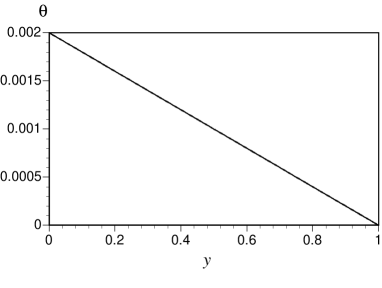
Figure 9: The numerical solution of $\theta(y)$ for $\theta(0)=0.002$ and $\theta(1)=0$. The parameters are $(b,c,e)=(3,7,7)$.

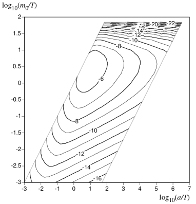
Figure 10: Contour plot of the chiral charge flux, normalized as $\log_{10}\left[-F_{Q}/(v_{w}T^{3}(Q_{L}-Q_{R}))\right]$ for the profile shown in Fig. 9. Here we take $v_{w}=0.58$ and $T=100\mbox{GeV}$.

As shown in Fig. 10, the magnitude of the chiral charge flux is reduced to about $O(10^{-3})$ of that in Fig. 7, which corresponds to the postulated profile (5.27) with maximal $CP$ violation. Hence, in this case, even if the forward-scattering is enhanced to give an extra factor of $O(10^{3})$ so that the baryon asymmetry is the optimal value (5.22), the parameter space is rather restricted to generate the present BAU only with the charge transport mechanism.

(ii) solution conserving $CP$ in the broken phase

In this case the boundary condition are $\theta_{0}=n\pi$ and $\theta_{1}=m\pi$. Then there are the trivial solution $\theta(y)=n\pi$ with the kink-type $\rho(y)$. Besides these, we found an interesting solution which violates $CP$ in the intermediate range near the bubble wall. If the effective potential admits the condition for the spontaneous $CP$ violation (6.8) to be satisfied for intermediate $v_{i}$, as shown in the contour plot of $V_{\rm eff}$ in Ref. [74], such a solution exists. Note that this condition is weaker than (6.25), which is required for spontaneous $CP$ violation in the broken phase region. Both conditions need $\lambda_{5}<0$. Unless the model has tree-level negative $\lambda_{5}$, it would be difficult to obtain negative $\lambda_{5}$ starting from $\lambda_{5}\geq 0$ at the tree-level, since only the fermions such as the gauginos in the MSSM contribute negatively to $\lambda_{5}$, while contributions from the bosons and fermions at finite temperature are positive. We present a solution of this type found in Ref. [74] and the chiral charge flux for it, in Fig. 11 and Fig. 12, respectively. This type of solution may exist for large $e$, which is the coefficient of $\rho^{3}\cos\theta$-term in the effective potential. As we noted earlier, the $\rho^{3}$-term arises from the boson loops whose mass at $\varphi=0$ vanishes. In the MSSM, the squark loop might give such a term if its mass is very small for $\varphi=0$.

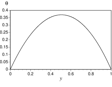
Figure 11: The numerical solution of $\theta(y)$ for $\theta(0)=\theta(1)=0$. The parameters are $(b,c,d,e)=(3,12.2,-2,12.2)$.

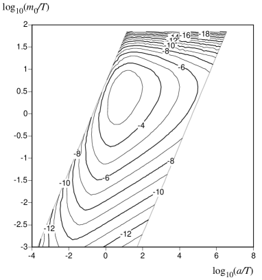
Figure 12: Contour plot of the chiral charge flux, normalized as $\log_{10}\left[-F_{Q}/(v_{w}T^{3}(Q_{L}-Q_{R}))\right]$ for the profile shown in Fig. 11. Here we take $v_{w}=0.58$ and $T=100\mbox{GeV}$.

Although the maximum of $\theta(y)$ is about $0.3$, the flux is comparable to that in Fig. 7, so that this profile could generate sufficient baryon asymmetry. Since this solution and the trivial solution $\theta(y)=0$ satisfy the same equation and the same boundary conditions, both would appear at the EWPT, but with different probabilities. One can determine the difference in the nucleation rate by comparing the free energy of the critical bubbles. The energy density per unit area of a bubble is given by

$${\cal E} = \int_{-\infty}^{\infty}dz\left\{{1\over 2}\sum_{i=1,2}\left[\left({{d\rho_{i}}\over{dz}}\right)^{2}+\rho_{i}^{2}\left({{d\theta_{i}}\over{dz}}\right)^{2}\right]+V_{\rm eff}(\rho_{1},\rho_{2},\theta)\right\}$$ (6.27)

$$= \int_{0}^{1}dy\left\{ay(1-y)\sum_{i=1,2}\left[\left({{d\rho_{i}}\over{dy}}\right)^{2}+\rho_{i}^{2}\left({{d\theta_{i}}\over{dy}}\right)^{2}\right]\right.$$

$$\qquad\qquad\qquad\left.+{1\over{2ay(1-y)}}V_{\rm eff}(\rho_{1},\rho_{2},\theta)\right\}.$$

The difference in the energy density is[74]

$$\Delta{\cal E}={\cal E}-\left.{\cal E}\right|_{\theta=0}=-2.056\times 10^{-3}\,av^{2}\sin^{2}\beta\cos^{2}\beta.$$ (6.28)

For the critical bubble of radius $R_{C}$, the $CP$-violating bubble will be nucleated with probability larger than the trivial one by the factor

$${\rm exp}\left(-{{4\pi R_{C}^{2}\Delta{\cal E}}\over{T_{C}}}\right).$$ (6.29)

According to the estimation in the massless two-Higgs-doublet model[39],  the radius of the critical bubble is given by $\sqrt{3F_{C}/(4\pi av^{2})}$, where $F_{C}$ is the free energy of the critical bubble and is found to be about $145T$. Then the exponent in (6.29) is $0.89\sin^{2}\beta\cos^{2}\beta$, irrespective of the wall width. For $\tan\beta=1$, the $CP$-violating bubbles are created about $1.22$ times more than the trivial ones.

Now we comment on the baryogenesis in the absence of explicit $CP$ violation. Since the effective potential is an even function of $\theta$, $-\theta(y)$ is also a solution to the equations of motion if $\theta(y)$ is. The energy densities of the both bubbles with $\theta(y)$ and $-\theta(y)$ — we refer to them as ‘positive bubble’ and ‘negative bubble’, respectively — are equal to each other. Thus their nucleation rates are also the same, so that the net generated baryon number will be zero on the average. This degeneracy of the energy density will be resolved once explicit $CP$ violation is taken into account. It was shown that in the MSSM, the explicit $CP$ violation in the soft supersymmetry breaking terms induces a $m_{3}^{2}$-type term proportional to $\sin\theta$ in the effective potential[72], If the difference in the free energy of the two bubbles is $\Delta F$, the ratio of their number will be

$${{N_{+}}\over{N_{-}}}={e}^{-\Delta F/T},$$ (6.30)

and the net baryon number is

$${{n_{B}}\over s}=\left({{n_{B}}\over s}\right)_{0}{{N_{+}-N_{-}}\over{N_{+}+N_{-}}}\simeq\left({{n_{B}}\over s}\right)_{0}{{\Delta F}\over T},$$ (6.31)

where $(n_{B}/s)_{0}$ is the baryon asymmetry generated by each bubble. Comelli et al. showed that the explicit $CP$ violation, which does not yield the neutron electric dipole moment beyond the experimental bound, splits the free energy as large as $\Delta F/T\simeq 10^{-2\sim-1}$[72]. If this is the case, the BAU is explained by the electroweak theory as long as $(n_{B}/s)_{0}\mathrel{\hbox{\raise 0.86108pt\hbox{$>$}\kern-7.5pt\raise-3.87495pt\hbox{$\sim$}}}10^{-9}$.

6.3 Solutions with explicit $CP$ violation

As we noted, explicit $CP$ violation is necessary to have nonzero baryon asymmetry. We found that even if it is very small, it nonperturbatively yields an energy gap between the positive and negative bubbles[75].

Here we consider only the phase in the $m_{3}^{2}$-term of the type $m_{3}^{2}({e}^{-i\delta}\Phi_{1}^{\dagger}\Phi_{2}+\mbox{h.c.})$, which is indeed induced in the MSSM. Then the equation for $\theta$ with the kink ansatz is now

$$y^{2}(1-y)^{2}{{d^{2}\theta(y)}\over{dy^{2}}}+y(1-y)(1-4y){{d\theta(y)}\over{dy}}$$

$$= b\sin(\delta+\theta(y))+\bigl{[}c(1-y)^{2}-e(1-y)\bigr{]}\sin\theta(y)+{d\over 2}(1-y)^{2}\sin(2\theta(y)),$$

where the parameters are defined by (6.24). Just as the case with spontaneous $CP$ violation above, the boundary conditions are determined by the parameters in the potential. We found two types of numerical solutions.

One type of solution is that of $\theta(y)=O(\delta)$ in the whole region and $\theta(1)=-\delta$. Note that $-\theta(y)$ is no longer a solution to (6.3). Hence there is no cancellation, but the generate baryon asymmetry would be the same order as that shown in Fig. 10, if $\delta=O(10^{-3})$.

The other solution is similar to that in Fig. 11, which connects $\theta(0)\simeq\delta$ and $\theta(1)=-\delta$ and grows to $\theta(y)\sim-0.6$ at $y\simeq 0.5$. For sufficiently small $\delta$ ($\sim 10^{-3}$), it has a partner satisfying the same boundary condition but with opposite sign in the intermediate region. For larger $\delta$, the partner can no longer exist. We calculated their energy density and found that for $\delta=0.0025$ and $(b,c,d,e)=(2.98005,12.178375,-2,12.2)$,

$$\Delta{\cal E}\equiv{\cal E}[\theta^{-}]-{\cal E}[\theta^{+}]=-1.917\times 10^{-2}av^{2}\sin^{2}\beta\cos^{2}\beta,$$ (6.33)

where $\theta^{-(+)}(y)$ denotes the solution with lower (higher) energy density. They are depicted in Fig. 13, which shows that $\theta^{\pm}(y)$ deviates from the solutions with $\delta=0$ by $O(0.1)$ near the bubble wall ($y\sim 0.5$) in spite of the small $\delta$.

Figure 13: The numerical solutions $\theta^{-}(y)$ (the dashed curve) and $\theta^{-}(y)$ (the dotted curve) for $\delta=0.0025$ and $(b,c,d,e)=(2.98005,12.178375,-2,12.2)$, which satisfy the boundary conditions, $\theta_{0}^{\pm}\simeq-0.311\delta$ and $\theta_{1}^{\pm}=-\delta$. The solid curves are the degenerate solutions for $\delta=0$ and $(b,c,d,e)=(3,12.2,-2,12.2)$ with $\theta_{0}=\theta_{1}=0$.

The ratio of the nucleation rates of the bubbles is

$${{N_{-}}\over{N_{+}}}=\exp\left(-{{4\pi R_{C}^{2}\Delta{\cal E}}\over{T_{C}}}\right)=8.05,$$ (6.34)

where we put $\tan\beta=1$. Then the net generated baryon asymmetry will be

$${{n_{B}}\over s}=\left({{n_{B}}\over s}\right)_{+}{{N_{+}}\over{N_{+}+N_{-}}}+\left({{n_{B}}\over s}\right)_{-}{{N_{-}}\over{N_{+}+N_{-}}}\simeq\left({{n_{B}}\over s}\right)_{+}{{N_{+}-N_{-}}\over{N_{+}+N_{-}}},$$ (6.35)

where we used $(n_{B}/s)_{-}\simeq-(n_{B}/s)_{+}$. Since the chiral charge flux for this profiles are expected to be the same order as that in Fig. 12, we will obtain sufficient baryon asymmetry.

All the solutions presented in this section are based on the kink ansatz. In fact, the solutions other than the trivial ones $\theta(y)=n\pi$ are not exact solutions to the full equations of motion. We also get solutions without this ansatz, which would have lower energy. In fact we found some numerical solutions, which have $\theta(y)$ of $O(1)$ so that $\rho_{i}(y)$ are no longer kink shape[77]. Such solutions may exist for a broader parameter region. We have concentrated on static solutions. If the EWPT accompanies exploding bubbles, we would need to solve the time-dependent equations, and if the viscosity of the medium cannot be ignored, we would have to solve the equations with frictions or random forces and then the wall profile might not give a monotonical $\rho$ like those obtained here. These extensions of the equations of motion are to be studied in the future.

7 Discussion

In this paper, we briefly reviewed the scenario of the electroweak baryogenesis. For it to be successful, some extensions of the MSM would be needed to have $CP$ violation in the Higgs sector. As one such model, we analyzed a two-Higgs-doublet model, including the MSSM, and tried to relate $CP$ violation to the baryon asymmetry generated at the EWPT. The main attraction of the electroweak baryogenesis is that it relies exclusively on physics which can be tested by present or near future experiments. In order to bridge the gap between detectable microphysics and the baryon asymmetry observed in the universe, we still have to know various aspects of the electroweak theory, in particular the EWPT and $CP$ violation in the model.

In principle, one can predict how much the baryon asymmetry is generated at the EWPT, once the renormalized lagrangian of the electroweak theory is given. From the lagrangian, one can construct the effective potential at finite temperature near the phase transition. One may use higher-order perturbation or nonperturbative methods such as the lattice simulation. As we saw in § 4, the studies have been limited to those of the MSM. We hope these efforts to be extended to the extended versions of the MSM. The effective potential gives information about the EWPT, such as its order, the transition temperature, and the latent heat and surface tension if it is first order. If the EWPT is not first order, the baryon number would be washed out except for the portion proportional to the primordial $B-L$. Even if the EWPT is first order, the unsuppressed sphaleron process would erase the baryon asymmetry. The Higgs mass is bounded from above, requiring that the EWPT be first order or that the sphaleron processes decouple after the EWPT. The upper bound seems inconsistent with the present lower bound of the Higgs scalar in the MSM. More detailed studies of the EWPT in the extended models will provide new constraints on the lightest Higgs boson. When the EWPT is first order, one can describe how the transition proceeds. If the phase transition accompanies nucleation and successive growth of the bubbles of the broken phase in the symmetric phase, the mechanisms presented in § 5 will yield the baryon asymmetry. The estimate of the generated baryon number depends on the velocity and thickness of the bubble wall and $CP$ violation around it, both of which should be dynamically determined.

When we analyzed the equations of motion for the Higgs fields in § 6, we did not completely fix the parameters in the potential. In practice, these are fixed once one chooses the model so that the type of profile is realized would also be determined. Under the assumptions made there, $\lambda_{5}<0$ might be necessary to have large $CP$ violation, while it may be a weaker condition for spontaneous $CP$ violation in the broken phase. Then a very small explicit $CP$ violation is needed to have nonzero net baryon asymmetry. In any case, if more detailed features of the EWPT in the two-Higgs-doublet model become available, one could calculate the generated baryon asymmetry, which in turn constrains some parameters in the model to explain the present BAU only with the help of the electroweak theory.

Appendix A Summary of the Big Bang Cosmology

In this appendix, we summarize the basics of the standard big bang cosmology and estimate various time scales at temperature near the electroweak phase transition. The most general form of homogeneous and isotropic space is the Friedmann-Robertson-Walker (FRW) metric, given by

$$ds^{2}=dt^{2}-R^{2}(t)\left[{{dr^{2}}\over{1-kr^{2}}}+r^{2}(d\theta^{2}+\sin^{2}\theta\,d\phi^{2})\right],$$ (A.1)

where $R(t)$ is the scale factor in the comoving coordinate. $k$ characterizes the topology of the space and $k=1,0,-1$ correspond to closed, flat and open space, respectively. The Einstein equation leads to

$$\left({{\dot{R}}\over R}\right)^{2}+{k\over{R^{2}}}-{\Lambda\over 3} = {{8\pi G_{N}}\over 3}\rho,$$ (A.2)

$${{\ddot{R}}\over R}-{\Lambda\over 3} = -{{4\pi G_{N}}\over 3}(\rho+3p),$$ (A.3)

where $\rho$ is the energy density, $p$ is the isotropic pressure, and $\Lambda$ is the cosmological constant. $\rho$ and $p$ are related by the equation of state; $p=\gamma\rho$, where $\gamma=1/3$ for a radiation-dominated universe and $\gamma\mathrel{<\kern-5.0pt<}1$ for a matter-dominated universe. Eliminating $\Lambda$ from (A.2) and (A.3), we have

$$(R^{3}\rho)^{\cdot}+3R^{2}{\dot{R}}p=0,$$ (A.4)

from which we obtain by use of the equation of state

$$\rho R^{3(\gamma+1)}=\mbox{constant}.$$ (A.5)

Because of

$$\int{{d^{3}{\mib k}}\over{(2\pi)^{3}}}\left|{\mib k}\right|{1\over{{e}^{\left|{\mib k}\right|/T}\mp 1}}=\left\{\begin{array}[]{l}\displaystyle{{{\pi^{2}}\over{30}}T^{4}},\\ \displaystyle{{7\over 8}{{\pi^{2}}\over{30}}T^{4}},\end{array}\right.$$ (A.6)

the energy density in a radiation-dominated universe is given by

$$\rho(T)={{\pi^{2}}\over{30}}g_{*}T^{4},$$ (A.7)

where $g_{*}$ represents the effective degrees of freedom at temperature $T$,

$$g_{*}\equiv\sum_{B}g_{B}+{7\over 8}\sum_{F}g_{F}.$$ (A.8)

Here $g_{B(F)}$ counts the spin and internal degrees of freedom of the bosons (fermions). For the standard model with $N_{f}$ generations and $m$ Higgs doublets,

$$g_{*}=24+4m+{7\over 8}\times 30N_{f},$$ (A.9)

so that $g_{*}=106.75$ for the MSM. In a radiation-dominated universe, the Hubble parameter is approximately given, from (A.2) with $\Lambda=0$, by

$$H\simeq\sqrt{{{8\pi G_{N}}\over 3}\rho}\simeq 1.66\sqrt{g_{*}}{{T^{2}}\over{m_{Pl}}},$$ (A.10)

where $m_{Pl}=\sqrt{G_{N}}=1.22\times 10^{19}\mbox{GeV}$ is the Planck mass.

The entropy density at present is related to the photon density as follows. As long as the local equilibrium is maintained, the law of thermodynamics implies

$$d(\rho_{i}V)=T_{i}dS_{i}-p_{i}dV+\mu_{i}dN_{i},$$ (A.11)

where the index $i$ denotes the particle species and $S_{i}$ is the entropy in a comoving volume $V$. This equation, together with the Gibbs-Duhem relation

$$S_{i}dT_{i}-Vdp_{i}+N_{i}d\mu_{i}=0,$$ (A.12)

lead to, up to a constant,

$$s_{i}\equiv{{S_{i}}\over{T_{i}}}={{\rho_{i}+p_{i}+\mu_{i}N_{i}/V}\over{T_{i}}}.$$ (A.13)

Neglecting the chemical potentials ($\mu_{i}\mathrel{<\kern-5.0pt<}T_{i}$), the entropy density is given by

$$s=\sum_{i}s_{i}=\sum_{i}{{\rho_{i}+p_{i}}\over T_{i}}.$$ (A.14)

Since the entropy is dominated by relativistic particles,

$$s={{2\pi^{2}}\over{45}}g_{*S}T^{3},$$ (A.15)

where

$$g_{*S}\equiv\sum_{B}g_{B}\left({{T_{B}}\over T}\right)^{3}+{7\over 8}\sum_{F}g_{F}\left({{T_{F}}\over T}\right)^{3}.$$ (A.16)

We can ignore the difference between $T_{i}$ and $T$ at high temperatures as shown below, while the difference is significant for $T<1\mbox{MeV}$. At such low temperatures, $\nu$-$\bar{\nu}$ annihilation decouples and the entropy in ${\rm e}^{\pm}$ pairs is transferred only to the photons. The entropy conservation implies

$$\left({{T_{\nu}}\over{T_{\gamma}}}\right)^{3}=g_{\gamma}/(g_{\gamma}+{7\over 8}g_{e})={4\over{11}}.$$ (A.17)

Hence today we have

$$g_{*S}=2+{7\over 8}\times{4\over{11}}\times 2\times 3=3.91,$$ (A.18)

which yields

$$s=7.04\cdot n_{\gamma}$$ (A.19)

with $n_{\gamma}$ being given by (A.21).

Now we shall estimate time scales of various interactions near $T_{C}\simeq 100\mbox{GeV}$ of the EWPT. Given a cross section $\sigma$ of some interaction, the mean free path $\lambda$ is estimated as

$$\lambda\cdot\sigma={1\over n},$$ (A.20)

where $n$ is the density of the particles which participate the interaction. At temperature $T$, $n$ of a massless particle whose degree of freedom is $g$ is

$$n=g\int{{d^{3}{\mib k}}\over{(2\pi)^{3}}}{1\over{{e}^{\left|{\mib k}\right|/T}\mp 1}}=\left\{\begin{array}[]{l}\displaystyle{{{\zeta(3)}\over{\pi^{2}}}gT^{3}},\\ \displaystyle{{3\over 4}{{\zeta(3)}\over{\pi^{2}}}gT^{3}},\end{array}\right.$$ (A.21)

where $\zeta(3)=1.2020569\cdots$. The mean free time $\bar{t}$ of a particle of mass $m$ and energy $E$ is given by

$${\bar{t}}={\lambda\over v}={\lambda\over{\sqrt{1-m^{2}/E^{2}}}}.$$ (A.22)

For $E\mathrel{>\kern-5.0pt>}m$, ${\bar{t}}\simeq\lambda$. Since the cross section of the interaction with the fine structure constant $\alpha$ at the center-of-mass energy $\sqrt{s}$ is $\sigma\simeq\alpha^{2}/s$, the mean free path at $T$ is

$$\lambda\simeq{{10}\over{g_{*}T^{3}}}\cdot{{T^{2}}\over{\alpha^{2}}}\simeq{1\over{10\alpha^{2}T}},$$ (A.23)

where we have used $g_{*}\simeq 100$ and $s\sim T^{2}$.

If we take $T=100\mbox{GeV}$,

$$\begin{array}[]{ll}\displaystyle{\lambda_{s}\simeq{1\over{10^{3}\alpha_{s}}}\sim 0.1\mbox{GeV}^{-1}}&\mbox{for strong interactions},\\ \displaystyle{\lambda_{EW}\simeq{1\over{10^{3}\alpha_{W}}}\sim 1\mbox{GeV}^{-1}}&\mbox{for electroweak interactions},\\ \displaystyle{\lambda_{Y}\simeq\left({{m_{W}}\over{m_{f}}}\right)^{4}\lambda_{EW}}&\mbox{for Yukawa interactions},\end{array}$$ (A.24)

where we have used $\alpha_{s}(m_{Z})=0.117\pm 0.005$ and $\alpha_{W}=\alpha_{QED}/\sin^{2}\theta_{W}\simeq 1/30$. At this temperature, the time scale of the universe expansion is, from (A.10),

$$H^{-1}(T)\simeq 10^{14}\mbox{GeV}^{-1}.$$ (A.25)

The time scale of the sphaleron process is

$${\bar{t}}_{\rm sph}\simeq(\Gamma_{\rm sph}/n)^{-1}\sim 10^{5}\mbox{GeV}^{-1}.$$ (A.26)

The thickness and velocity of the bubble nucleated at the EWPT are

$$l_{w}\simeq{{1\sim 40}\over T}\simeq 0.01\sim 0.4\mbox{GeV}^{-1}$$ (A.27)

and

$$v_{w}\simeq 0.1\sim 0.9,$$ (A.28)

respectively[49]. Although $l_{w}$ and $v_{w}$ are correlated, we adopt as the scale of the EWPT,

$$t_{\rm wall}={{l_{w}}\over{v_{w}}}\simeq 0.01\sim 4\mbox{GeV}^{-1}.$$ (A.29)

From these we see the following:

1. All the particles are in kinetic equilibrium at the same temperature, because of $H^{-1}\mathrel{>\kern-5.0pt>}{\bar{t}}_{EW}$, far from the bubble wall.

2. The Yukawa interactions of the light fermions ($m_{f}<0.1\mbox{GeV}$) are out of chemical equilibrium.

3. Some of the flavor-changing interactions are out of chemical equilibrium because of small KM matrix elements.

4. Since for the leptons $\lambda_{Y}>\lambda_{EW}\mathrel{>\kern-5.0pt>}l_{w}$, the leptons propagate almost freely before and after the scattering off the bubble wall.

5. Because of $t_{\rm wall}\mathrel{<\kern-5.0pt<}{\bar{t}}_{\rm sph}$, the sphaleron process is out of chemical equilibrium near the bubble wall.

Appendix B Derivation of the Baryon-Number-Changing Rate

Suppose that there are states with discrete labels, $i$. Let $P(i;t)$ be the probability to find the system in the state $i$ at time $t$, and $\Gamma_{i\rightarrow j}$ be the transition probability from state $i$ to $j$ per unit time. Then the following master equation holds:

$$P(i;t+\Delta t)=-\sum_{j\not=i}P(i;t)\Gamma_{i\rightarrow j}\Delta t+\sum_{j\not=i}P(j;t)\Gamma_{j\rightarrow i}\Delta t+P(i;t).$$ (B.1)

For a steady state, detailed balance is maintained, that is, $P(i;t)$ is independent of $t$; $P(i;t)=P_{\rm eq}(i)$ for any $t$. Then (B.1) is reduced to the detailed balance equation;

$$\sum_{j\not=i}P_{\rm eq}(i)\Gamma_{i\rightarrow j}=\sum_{j\not=i}P_{\rm eq}(j)\Gamma_{j\rightarrow i}.$$ (B.2)

This implies for the case of baryon number changing processes

$$\sum_{n=1}^{\infty}P_{\rm eq}(B)\left(\Gamma_{B\rightarrow B+n}+\Gamma_{B\rightarrow B-n}\right)$$ (B.3)

$$= \sum_{n=1}^{\infty}\left[P_{\rm eq}(B+n)\Gamma_{B+n\rightarrow B}+P_{\rm eq}(B-n)\Gamma_{B-n\rightarrow B}\right],$$

where $P_{\rm eq}(B)\propto{e}^{-F_{B}/T}$ with $F_{B}$ being the free energy of the state with baryon number $B$. The transition rates with $\Delta B=\pm 1$ are given by $\Gamma_{+}=\Gamma_{B\rightarrow B+1}$ and $\Gamma_{-}=\Gamma_{B\rightarrow B-1}$ and the others are approximated by $\Gamma_{B\rightarrow B+n}\simeq\Gamma_{+}^{n}$ and $\Gamma_{B\rightarrow B-n}\simeq\Gamma_{-}^{n}$. Since $F_{B+n}=F_{B}+n\mu_{B}$, (B.3) yields

$$\sum_{n=1}^{\infty}\left[\Gamma_{+}^{n}+\Gamma_{-}^{n}\right]\simeq\sum_{n=1}^{\infty}\left[({e}^{-\mu_{B}/T}\Gamma_{-})^{n}+({e}^{\mu_{B}/T}\Gamma_{+})^{n}\right].$$ (B.4)

If $\Gamma_{\pm}\mathrel{<\kern-5.0pt<}1$, only the contribution from $n=1$ in the sum is dominant so that $\Gamma_{+}+\Gamma_{-}\simeq{e}^{-\mu_{B}/T}\Gamma_{-}+{e}^{\mu_{B}/T}\Gamma_{+}$, which leads to

$${{\Gamma_{+}}\over{\Gamma_{-}}}\simeq{e}^{-\mu_{B}/T}.$$ (B.5)

By definition, ${\dot{n}}_{B}=\Gamma_{+}-\Gamma_{-}$ if we use $\Gamma_{\pm}$ as the rate per unit volume and unit time. That is approximately given by the sphaleron rate, $\Gamma_{+}\sim\Gamma_{-}\simeq\Gamma_{\rm sph}$. Hence we have

$${\dot{n}}_{B}=\Gamma_{-}\left({{\Gamma_{+}}\over{\Gamma_{-}}}-1\right)\simeq\Gamma_{\rm sph}({e}^{-\mu_{B}/T}-1)\simeq-{{\Gamma_{\rm sph}\mu_{B}}\over T}.$$ (B.6)

References

- [1] E.D. Kolb and M.S. Turner, The Early Universe (Addison-Wesley Publishing, 1990).
- [2] Particle Data Group, Phys. Rev. D50 (1994) 1173 and 1995 off-year partial update for the 1996 edition available on the PDG WWW pages (URL: http://pdg.lbl.gov/). Especially, see the ‘Astrophysics and Cosmology’ section in “Reviews, Tables, and Plots”.
- [3] A.D. Sakharov, JETP Lett., 5 (1967) 24.
- [4] M. Yoshimura, Phys. Rev. Lett. 41 (1978) 281, (E)42 (1978), 746.
- [5] E.D. Kolb and M.S. Turner, Ann. Rev. Nucl. Part. Sci., 33 (1983) 645 and references therein.
- [6] A. Cohen, D. Kaplan and A. Nelson, Ann. Rev. Nucl. Part. Sci.,43 (1993) 27.
- [7] V. A. Kuzmin, V. A. Rubakov and M. E. Shaposhnikov, Phys. Lett. 155B (1985) 36.
- [8] M. Fukugita and T. Yanagida, Phys. Lett. B174 (1986) 45.
-
[9]
I. Affleck and M. Dine, Nucl. Phys. B249 (1985) 361.
M. Dine, L. Randall and S. Thomas, Nucl. Phys. B458 (1996) 291. - [10] R. H. Brandenberger and A.-C. Davis, Phys. Lett. B308 (1993) 79.
- [11] For a review on the anomaly, see, R. Jackiw, Topological Investigations of Quantized Gauge Theories in Relativity, Groups and Topology II, Les Houches 1983, ed. B. S. DeWitt and R. Stora (North Holland, Amsterdam, 1984).
- [12] A. A. Belavin, A. M. Polyakov, A. S. Schwarz and Yu. S. Tyupkin, Phys. Lett. 59B (1975) 85.
- [13] G. ’t Hooft; Phys. Rev. D14 (1976) 3432, (E) D18 (1978) 2199; Phys. Rep.,142 (1986) 357.
- [14] R. Jackiw and C. Rebbi, Phys. Rev. Lett. 37 (1976) 172.
- [15] I. Affleck, Nucl. Phys. B191 (1981) 429.
- [16] V. V. Khoze and A. Ringwald, Nucl. Phys. B355 (1991) 351.
- [17] K. Fujikawa, Phys. Rev. Lett. 42 (1979) 1195.
-
[18]
C. Callan, R. F. Dashen and D. J. Gross,
Phys. Rev. D17 (1978) 2717.
J. Kiskis, Phys. Rev. D18 (1978) 3690.
N. Christ, Phys. Rev. D20 (1980) 1591.
J. Ambjorn, J. Greensite and C. Peterson, Nucl. Phys. B221 (1983) 381. - [19] N. S. Manton, Phys. Rev. D28 (1983) 2019.
- [20] F. R. Klinkhamer and N. S. Manton, Phys. Rev. D30 (1984) 2212.
- [21] R. Forgács and Z. Horváth, Phys. Lett. 138B (1984) 397.
- [22] A. I. Bocharev and M. E. Shaposhnikov, Mod. Phys. Lett., A2 (1987) 991.
-
[23]
E. Mottola and A. Wipf, Phys. Rev. D39 (1989) 588.
K. Funakubo, S. Otsuki and F. Toyoda, Prog. Theor. Phys. 83 (1990) 118. - [24] Y. Brihaye and J. Kunz, Phys. Rev. D50 (1994) 4175.
- [25] I. Affleck, Phys. Rev. Lett. 46 (1981) 388.
- [26] J. S. Langer, Ann. Phys. 41 (1967) 108; 54 (1969) 258.
- [27] C. G. Callan and S. Coleman, Phys. Rev. D16 (1977) 1762.
- [28] P. Arnold and L. McLerran, Phys. Rev. D36 (1987) 581.
-
[29]
T. Akiba, H. Kikuchi and T. Yanagida,
Phys. Rev. D40 (1989) 588.
L. Carson and L. McLerran, Phys. Rev. D41 (1990) 647.
L. Carson, X. Li and L. McLerran, Phys. Rev. D42 (1990) 2127. - [30] J. Ambjørn, T. Askgaard, H. Porter and M.E. Shaposhnikov, Nucl. Phys. B353 (1991) 346.
- [31] J. Ambjørn and A. Krasnitz, Phys. Lett. B362 (1995) 97.
- [32] J. Havey and M. S. Turner, Phys. Rev. D42 (1990) 3344.
-
[33]
H. Dreiner and G. G. Ross, Nucl. Phys. B410 (1993) 188.
T. Inui, T. Ichihara, Y. Mimura and N. Sakai, Phys. Lett. B325 (1994) 392. - [34] D. A. Kirzhnits and A. D. Linde, Ann. Phys. 101 (1976) 195.
- [35] L. Dolan and R. Jackiw, Phys. Rev. D9 (1974) 3320.
- [36] M. Sher, Phys. Rep., 179 (1989) 273.
- [37] M. Dine, R. G. Leigh, P. Huet, A. Linde and D. Linde, Phys. Rev. D46 (1992) 550.
- [38] M. E. Shaposhnikov, JETP Lett., 44 (1986) 465; Nucl. Phys. B287 (1987) 757; B299 (1988) 797.
- [39] K. Funakubo, A. Kakuto and K. Takenaga, Prog. Theor. Phys. 91 (1994) 341.
- [40] A. T. Davis, C. D. Froggatt, G. Jenkins and R. G. Moorhouse, Phys. Lett. B336 (1993) 464.
- [41] S. Myint, Phys. Lett. B287 (1992) 325.
- [42] P. Arnold and O. Espinosa, Phys. Rev. D47 (1993) 3546.
- [43] J. Kripfganz, A. Laser and M. G. Schmidt, Phys. Lett. B351 (1995) 266.
- [44] Z. Fodor and A. Hebecker, Nucl. Phys. B432 (1994) 127.
- [45] For a review of lattice simulation, see C. Rebbi, Lattice Gauge Theories and Monte Carlo Simulations (World Scientific, Singapore, 1983).
-
[46]
K. Kajantie, M. Laine, K. Rummukainen and
M. Shaposhnikov, Nucl. Phys. B458 (1996) 90.
K. Farakos, K. Kajantie, K. Rummukainen and M. Shaposhnikov, Nucl. Phys. B442 (1995) 317. - [47] S. Elitzur, Phys. Rev. D12 (1975) 3978.
- [48] K. Jansen, plenary talk given at LATTICE ‘95, Nucl. Phys. B (Proc. Suppl.), 47 (1996) 196.
- [49] B. Liu, L. McLerran and N. Turok, Phys. Rev. D46 (1992) 2668.
- [50] G. Moore and T. Prokopec, Phys. Rev. Lett. 75 (1995) 777.
- [51] M. E. Carrington and J. I. Kapsta, Phys. Rev. D47 (1993) 5304.
-
[52]
M. Gleiser, E. W. Kolb and R. Watkins,
Nucl. Phys. B364 (1991) 411.
G. Gelmini and M. Gleiser, Nucl. Phys. B419 (1994) 129.
M. Gleiser, Phys. Rev. Lett. 73 (1994) 3495.
T. Shiromizu, M. Morikawa and J. Yokoyama, Prog. Theor. Phys. 94 (1995) 795. - [53] G. R. Farrar and M. E. Shaposhnikov, Phys. Rev. Lett. 70 (1993) 2833; Phys. Rev. D50 (1994) 774.
- [54] A. E. Nelson, D. B. Kaplan and A. G. Cohen, Nucl. Phys. B373 (1992) 453.
- [55] K. Funakubo, A. Kakuto, S. Otsuki, K.Takanaga and F. Toyoda, Phys. Rev. D50 (1994) 1105; Prog. Theor. Phys. 93 (1995) 1067.
-
[56]
M. B. Gavela, M. Lozano, J. Orloff and O. Pène,
Nucl. Phys. B430 (1994) 345.
M. B. Gavela, P. Hernandez, J. Orloff, O. Pène and C. Quimbay, Nucl. Phys. B430 (1994) 382.
P. Huet and E. Sather, Phys. Rev. D51 (1995) 379. - [57] M. Joyce, T. Prokopec and N. Turok, Phys. Lett. B338 (1994) 269.
- [58] K. Funakubo, A. Kakuto, S. Otsuki and F. Toyoda, Prog. Theor. Phys. 95 (1996) 929.
- [59] N. Turok and J. Zadrozny, Phys. Rev. Lett. 65 (1990) 2331.
- [60] L. McLerran, M. Shaposhnikov, N. Turok and M. Voloshin, Phys. Lett. B256 (1991) 451.
- [61] A. G. Cohen, D. B. Kaplan and A. E. Nelson, Phys. Lett. B263 (1991) 86.
- [62] M. Dine and S. Thomas, Phys. Lett. B328 (1994) 73.
- [63] A. G. Cohen, D. B. Kaplan and A. E. Nelson, Phys. Lett. B336 (1994) 41.
- [64] M. Joyce, T. Prokopec and N. Turok, Phys. Rev. D53 (1996) 2930; D53 (1996) 2958.
- [65] J. F. Gunion, H. E. Haber, G. Kane and S. Dawson, The Higgs Hunter’s Guide, (Addison-Wesley Publishing, 1990).
- [66] S. L. Glashow and S. Weinberg, Phys. Rev. D15 (1977) 1958.
- [67] Y. L. Wu and L. Wolfenstein, Phys. Rev. Lett. 73 (1994) 1762; 73 (1994) 2809.
- [68] L. M. Krauss and S. J. Rey, Phys. Rev. Lett. 69 (1992) 1308.
- [69] N .Maekawa, Phys. Lett. B282 (1992) 392; Nucl. Phys. B (Proc. Suppl.), 37A (1994) 191.
- [70] H. Georgi and A. Pais, Phys. Rev. D10 (1974) 1246.
- [71] D. Comelli, M. Pietroni, Phys. Lett. B306 (1993) 67.
- [72] D. Comelli, M. Pietroni and A. Riotto, Nucl. Phys. B412 (1994) 441.
- [73] J. R. Espinosa, J. M. Moreno and M. Quirós, Phys. Lett. B319 (1993) 505.
- [74] K. Funakubo, A. Kakuto, S. Otsuki, K.Takanaga and F. Toyoda, Prog. Theor. Phys. 94 (1995) 845.
- [75] K. Funakubo, A. Kakuto, S. Otsuki and F. Toyoda, hep-ph/9606282, to be published in Prog. Theor. Phys. 96 No. 4.
- [76] J. M. Cline, K. Kainulainen, and A. P. Vischer, Phys. Rev. D54 (1996) 2451.
- [77] K. Funakubo, A. Kakuto, S. Otsuki and F. Toyoda, in preparation.