FERMILAB - CONF - 96 - 224 - T

GLUON DENSITY IN NUCLEI
A. L. Ayala F${}^{\underline{o}}$ ${}^{a)\,b)}$^∗ , M. B. Gay Ducati ^a)∗∗ and E. M. Levin ${}^{c)\,d)\,\dagger}$

^a)Instituto de Física, Univ. Federal do Rio Grande do Sul
Caixa Postal 15051, 91501-970 Porto Alegre, RS, BRAZIL
^b)Instituto de Física e Matemática, Univ. Federal de Pelotas
Campus Universitário, Caixa Postal 354, 96010-900, Pelotas, RS, BRAZIL
^c) Theory Division, Fermi National Accelerator Laboratory
Batavia, IL 60510 - 0500, USA

^d) Theory Department, Petersburg Nuclear Physics Institute
188350, Gatchina, St. Petersburg, RUSSIA
Talk, given by E.M. Levin at RHIC’96 Summer Study, BNL, LI, July 7 - 19, 1996

Abstract: In this talk we present our detail study ( theory and numbers ) [1] on the shadowing corrections to the gluon structure functions for nuclei. Starting from rather contraversial information on the nucleon structure function which is originated by the recent HERA data, we develop the Glauber approach for the gluon density in a nucleus based on Mueller formula [3] and estimate the value of the shadowing corrections in this case. Than we calculate the first corrections to the Glauber approach and show that these corrections are big. Based on this practical observation we suggest the new evolution equation which takes into account the shadowing corrections and solve it. We hope to convince you that the new evolution equation gives a good theoretical tool to treat the shadowing corrections for the gluons density in a nucleus and, therefore, it is able to provide the theoretically reliable initial conditions for the time evolution of the nucleus - nucleus cascade. The initial conditions should be fixed both theoretically and phenomenologically before to attack such more complicated problems as the mixture of hard and soft processes in nucleus-nucleus interactions at high energy or the theoretically reliable approach to hadron or/and parton cascades for high energy nucleus-nucleus interaction.

1 Introduction.

The main goal of this talk is to share with you our experience and results that we got during the last two years reconsidering the whole issue of the shadowing corrections ( SC ) to the gluon density in nuclei [1]. The title which reflects the key problems that we are going to discuss is: “ All ( theory and numbers ) about the SC to gluon density in nuclei”

It is well known that the gluon density is the most important physical observable that governs the physics at high energy (low Bjorken $x$) in deep inelastic processes [2]. Dealing with nucleus we have to take into account the shadowing correction (SC) due to rescattering of the gluon inside the nucleus, which is the main point of interest in this paper. We show that SC can be treated theoretically in the framework of perturbative QCD (pQCD) and can be calculated using the information on the behavior of the gluon structure function for the nucleon.

The outline of the talk looks as follows. We start with our motivation answering the question why we got interested in the SC for nucleus gluon density. In section 3 we will discuss the theory and numerics of the Glauber ( Mueller ) approach emphasizing it’s theory status and the estimates for the SC that came out of it. After short discussion in section 4 the first corrections to the Glauber approach we will present what we consider as a right way of doing, namely, the new evolution equation that sums all SC ( section 5 ). In section 6 we are going to discuss our next steps that we plan to do in a nearest future, while in section 7 we will give our answer to the hot question: and what ?, trying to collect all problems of RHIC physics that we will be able to answer using our approach.

2 Motivation.

Let us start with a brief summary of the HERA results for the nucleon structure functions ( parton densities in a nucleon). The experiment [4] shows that the deep inelastic structure function $F_{2}(x,Q^{2})$ increases in the region of small $x$ ( at high energies):

$$F_{2}(x,Q^{2})\,\,\propto\,\,\frac{1}{x^{0.2}}\,\,\,\,\,\,for\,\,\,\,\,\,10^{-2}\,\,>\,\,x\,\,>\,\,10^{-5}$$

at large and small ( $Q^{2}\,\approx\,1\,-\,2\,GeV^{2}$ ) values of the photon virtualities $Q^{2}$.

At first sight we can conclude from the analysis based on the DGLAP evolution equations undertaken through all the world R[6] [7] [8] that :

1. The DGLAP evolution equations work quite well and no other ingredients are needed to describe all the HERA data.

2. The parton cascade is rather deluted system of partons with small parton - parton interaction which can be neglected in a first approximation. In other words we do not need any SC to describe the experimental data.

3. The phenomenological input, namely, the quark and gluon distribution at initial virtuality $Q^{2}=Q^{2}_{0}$ can be chosen at sufficiently low values of $Q^{2}$ using the backward evolution of the experimental data in the region of $Q^{2}\,\approx\,4-5GeV^{2}$. Even more, the craziest parameterization that we have seen in our life - the GRV one [6] does it’s job perfectly well, starting with $Q^{2}_{0}=0.3GeV^{2}$ ?!.

What we have discussed is moreless common opinion of all experts in DIS and one can find it in many plenary and review talks during the last two years.

However we would like to draw your attention to several facts which do not fit to this common scheme:

1. The best parameterization of the HERA data is not the solution of the DGLAP equations but a simple formula [9]:

$$F_{2}(x,Q^{2})\,\,=\,\,a\,\,+\,\,m\,\log\frac{Q^{2}}{Q^{2}_{0}}\,\log\frac{x_{0}}{x}$$

with $a$ = 0.078 ; $m$ = 0.364 ; $x_{0}$ = 0.074 ; $Q^{2}_{0}$  = 0.5 $GeV^{2}$. It is clear that this simple formula cannot be a solution of the DGLAP evolution equations. To make obvious this remark it is enough to recalculate the gluon structure function from the above expression as it has been done in Ref.[9]. Indeed, $xG(x,Q^{2})$ turns out to be equal to

$$xG(x,Q^{2})\,\,=\,\,3\,\,\log\frac{x_{0}}{x}$$

without any $Q^{2}$ - dependence within the direct contradiction with the DGLAP evolution.

2. Using the HERA data we can evaluate the parameter which characterizes the value of the SC, namely [2]

$$\kappa\,\,=\,\,\frac{3\,\pi\,\alpha_{\rm S}}{Q^{2}\,R^{2}}\,\,xG(x,Q^{2})\,\,,$$ (1)

where $xG(x,Q^{2})$ is the gluon structure function and $R^{2}$ is the radius of area populated by gluons in a nucleon. The physical meaning of $\kappa$ becomes clear if we rewrite it in the form

$$\kappa\,\,=\,\,xG(x,Q^{2})\,\frac{\sigma(GG)}{\pi\,R^{2}}\,\,,$$

where $\sigma(GG)$ is the cross section of two gluon interaction in our parton cascade calculated by Mueller and Qiu [10], namely, $\sigma(GG)\,\,=\,\,\frac{3\pi^{2}\alpha_{\rm S}}{Q^{2}}$. The physical meaning of this formula is the probability of the gluon - gluon interaction inside the parton cascade. It looks very natural if we compare eq. (1) with the small parameter for proton - nucleus interaction. Indeed, the parameter which governs the value of the Glauber corrections for proton - nucleus interaction $\kappa_{pA}\,=\,A\frac{\sigma(pp)}{\pi R^{2}_{A}}$, where $A$ is the number of the constituents (nucleons) , $\sigma(pp)$ is the cross section of the interaction of our constituents and $\pi R^{2}_{A}$ is the area populated by nucleons. The question arises what is the value of $R$ in eq. (1)?

Figure 1: The $J/\Psi$ production without a) and with b) dissociation of the proton.

Using the new HERA data on photoproduction of J/$\Psi$ meson [11] we are able to estimate the value of $R^{2}$ in the definition of $\kappa$ (see eq. (1) ). To illustrate the point we picture in Fig.1 the process of J/$\Psi$ photoproduction in the additive quark model (AQM ). We see that we have two processes with different slopes ($B$ ) in $t$ ( or in $b^{2}_{\perp}$ ): the J/$\Psi$ production without ( Fig.1a ) ($B_{el}\,=\,5\,GeV^{-2}$) and with ( Fig.1b ) ( $B_{in}\,=\,1.66\,GeV^{-2}$ ) dissociation of the proton. The AQM gives us the simplest estimates for the resulting slope ( $R^{2}$ ) in eq. (1) if we neglect any slope from the Pomeron - J/$\Psi$ vertex in Fig.1, namely

$$\frac{1}{R^{2}}\,\,=\,\,\frac{1}{4}\,\{\,\frac{3}{2B_{el}}\,\,+\,\,\frac{1}{2B_{in}}\,\}\,\,\approx\,\,\frac{1}{5}\,GeV^{-2}\,\,.$$ (2)

Figure 2: Contour plot for $\kappa$ for $R^{2}=\,5Gev^{-2}$.

Fig.2 shows the contour plot for $\kappa$ using the GRV parameterization [6] for the gluon structure function and the value of $R^{2}=5GeV^{-2}$. One can see that $\kappa$ reaches $\kappa$ = 1 at HERA kinematic region, meaning shadowing corrections take place.

3. The situation looks even more contraversparameterizationial if we plot the average value of the anomalous dimension $<\gamma>\,\,=\,\,\partial\ln(xG(x,Q^{2}))/\partial\ln Q^{2}$ in the GRV parameterization. Fig.3 shows two remarkable lines: $<\gamma>=1$, where the deep inelastic cross section reaches the value compatible with the geometrical size of the proton, and $<\gamma>\,=\,1/2$, which is the characteristic line in whose vicinity both the BFKL Pomeron ( see Ref.[12] ) and the GLR equation [2] should take over the DGLAP evolution equations.We will discuss later what are the BFKL and the GLR equations, what we need to know right now, is only the fact that both equations give the signal of the new physics. The HERA data passed over the second line and even for sufficiently small values of $Q^{2}$ they crossed the first one without any indication of a strange behaviour near these lines.

Figure 3: Contours for $<\gamma>$ = 1 and $<\gamma$ = 1/2.

Concluding this brief summary of the HERA data and physics behind them we would like to repeat that to our taste the situation at HERA looks very controversial and the statement that the DGLAP evolution works is first but not the last outcome of the HERA data. On the other hand we have to develop the new approach to the SC, more general than the GLR one, which will allow us to give reliable estimates for the SC in the kinematic region to the left of the line $<\gamma>\,=\,1/2$. This is why we decided to reconsider everything that has been known about the SC, trying to forget everything that we knew about them, and to start our analisys of the SC from the very beginning. We also decide to choose the gluon density in a nucleus as a laboratory or training ground for the new approach to the problem of the SC.

We have three reasons for such a choice: (i) the nucleus DIS is easier to handle theoretically, as we will show in the main body of our talk;(ii) the previous analysis of the SC shows that this is mainly density effect in the parton cascade ( see review [13] for example ) and we anticipate larger gluon density for DIS with a nucleus; (iii) the RHIC is coming and the gluon density in nuclei will provide the initial condition for any phenomenological cascades for nucleus - nucleus interaction at high energies.

Figure 4: The structure of the parton cascade in the Glauber ( Mueller) formula. $A$ denotes the nucleus, N - the nucleon, $G^{*}(Q^{2})$ - the virtual gluon and $\sigma_{N}(r^{2}_{t})$ is the nucleon cross section.

3 The Glauber approach in QCD .

3.1 The Mueller formula.

The idea how to write the Glauber formula in QCD was originally formulated in two papers Ref.[14] and Ref. [3]. However, the key paper for our problem is the second paper of A. Mueller who considered the Glauber approach for the gluon structure function. Nevertheless, it is easier to explain the main idea considering the penetration of quark - antiquark pair, produced by the virtual photon, through the target. While the boson projectile is traversing the target, the distance $r_{\perp}$ between the quark and anti-quark can vary by amount $\Delta r_{\perp}\propto R_{A}\frac{k_{t}}{E}$ where $E$ denotes the energy of the pair in the target rest frame and $R_{A}$ is the size of the target (see Fig.4). The quark transverse momentum is $k_{t}\propto 1/r_{\perp}$. Therefore

$$\Delta\,r_{\perp}\,\propto\,R\,\,\frac{k_{t}}{E}\,\,\ll\,\,r_{\perp}\,,$$ (3)

and is valid if

$$\,r^{2}_{\perp}\,s\,\,\gg\,\,\,2\,m\,R\,,$$ (4)

where $s=2mE$. In terms of Bjorken $x$, the above condition looks as follows

$$x\,\,\ll\,\,\frac{1}{2\,m\,R}\,.$$ (5)

Therefore the transverse distance between quark and antiquark is a good degree of freedom [14][3][17]. As has been shown by A.Mueller, not only quark - antiquark pairs can be considered in a such way. The propagation of a gluon through the target can be treated in a similar way as the interaction of gluon - gluon pair with definite transverse separation $r_{t}$ with the target. It is easy to understand if we remember that virtual colorless graviton or Higgs boson is a probe of the gluon density.

The total cross section of the absorption of gluon($G^{*}$) with virtuality $Q^{2}$ and Bjorken $x$ can be written in the form:

$$\sigma^{A}_{tot}(\,G^{*}\,)\,\,=\,\,\int^{1}_{0}dz\,\,\int\,\frac{d^{2}r_{t}}{2\pi}\,\,\int\frac{d^{2}b_{t}}{2\pi}\Psi^{G^{*}}_{\perp}(Q^{2},r_{t},x,z)\,\,\sigma_{A}(x,r^{2}_{t})\,\,\,\,[{\Psi^{G^{*}}_{\perp}}(Q^{2},r_{t},x,z)]^{*}\,,$$ (6)

where $z$ is the fraction of energy which is carried by the gluon, $\Psi^{G^{*}}_{\perp}$ is the wave function of the transverse polarized gluon and $\sigma_{A}(x,r^{2}_{t})$ is the cross section of the interaction of the $GG$- pair with transverse separation $r_{t}$ with the nucleus. This cross section can be written in the form:

$$\sigma_{A}(x,r^{2}_{\perp})\,\,=\,\,2\,\int\,d^{2}b_{t}\,Ima(x,r_{\perp},b_{t})\,\,,$$ (7)

where $a$ is the elastic amplitude for which we have the $s$-channel unitarity constraint:

$$2\,\,Im\,a(x,r_{\perp},b_{t})\,\,=\,\,|a(x,r_{\perp},b_{t})|^{2}\,\,+\,\,G_{in}(x,r_{\perp},b_{t})\,,$$ (8)

where $G_{in}$ is the contribution of all the inelastic processes. Let us recall that two terms in eq. (8) have different physical meaning: the left hand side and the first term in the right hand side describe the interference between the incoming plane wave and outgoing spherical wave which amplitude is the elastic scattering amplitude ($a$). These two terms cannot be calculated using a classical approach or simple Monte Carlo - like model. The Quantum Mechanics of the interaction is mostly absorbed in these two terms while the last term has a simple probabilistic meaning, namely, the probability of any inelastic interactions, and can be treated almost classically and, for certain, in the probabilistic way, for example in Monte Carlo-like models. The unitarity establishes the correlation between two unknowns $a$ and $G_{in}$ and has the general solution:

$$a(x,r_{\perp},b_{t})\,\,=\,\,i\,\{\,\,1\,\,-\,\,e^{-\,\frac{1}{2}\,\Omega(x,r_{\perp},b_{t})}\,\,\}\,\,;$$ (9)

$$G_{in}(x,r_{\perp},b_{t})\,\,=\,\,1\,\,-\,\,e^{-\,\Omega(x,r_{\perp},b_{t})}\,\,.$$

One can see that $\Omega$ has a simple physical meaning, namely $e^{-\Omega}$ is the probability that $GG$-pair has no inelastic interaction during the passage through the target. The opacity $\Omega$ is an arbitrary real function, which can be specified only in more detail theory or model approach than the unitarity constraint. One of such specific model is Glauber approach or Eikonal model.

However, before we will discuss this model let us make one important remark on the strategy of the approach to the SC. We are trying to built a model or theory for the total cross section ( or for the gluon structure function ) not because the SC should be the strongest one in this particular observable, but because if we will be able to calculate opacity $\Omega$ we will have the theory or model for all inelastic processes. Indeed, using AGK cutting rules [15] we can calculated any inelastic process, if we know $\Omega$, in accordance with the $s$-channel unitarity. It is worthwhile mentioning that the inverse procedure does not work. If we know the SC in all details for a particular inelastic process, say for the inclusive production, we cannot reconstruct all other process and the total cross section in particular.

Now, let us built the Glauber approach. First, let us assume that $\Omega$ is small ($\Omega\,\,\ll\,\,1$ ) and it’s $b_{t}$ dependence can be factorised as $\Omega\,=\,\widetilde{\Omega}(x,r_{\perp})\,S(b_{t})$ with the normalization: $\int\,d^{2}b_{t}\,S(b_{t})\,=\,1$. Expanding eq. (9) and substituting it in eq. (7), one can obtain:

$$\sigma_{A}(x,r_{\perp})\,\,=\,\,\widetilde{\Omega}(x,r_{\perp})$$ (10)

At small $\Omega$ the cross section of the deep inelastic process with a nucleus is proportional to the number of nucleons in a nucleus ($A$), namely,

$$\sigma_{A}(x,r_{\perp})\,\,=\,\,A\,\sigma_{N}(x,r_{\perp}).$$

To calculate $\widetilde{\Omega}$ we need to substitute everything in eq. (6) and use the formula for $\sigma_{A}(\,G^{*})\,\,=\,\,\frac{4\pi^{2}}{Q^{2}}xG_{A}(x,Q^{2})$ as well as the expression for the wave function of the $GG$- pair in the virtual gluon probe. Such calculations has been done in Ref.[3] and we recapture here the result ( see for example Ref. [1] for more details ):

$$\widetilde{\Omega}\,\,=\,\,A\,\sigma_{N}(x,r_{\perp})\,\,=\,\,\frac{3\,\pi^{2}}{4}\,\,r^{2}_{\perp}\,xG(x,\frac{4}{r^{2}_{\perp}})\,\,.$$ (11)

The Glauber (eikonal ) approach is the assumption that $\Omega\,=\,\widetilde{\Omega}\,S(b_{t})$ with $\widetilde{\Omega}$ of eq. (11) not only in the kinematic region where $\Omega$ is small but everywhere. From the point of view of the structure of the final state this assumption means that the rich typical inelastic event was modeled as a sum of the diffraction dissociation of $GG$ - pair plus uniform in rapidity distribution of produced gluons. For example, we neglected in the Glauber approach all rich structure of the large rapidity gap events including the diffractive dissociation in the region of large mass.

Substituting everything in eq. (11) and eq. (6) and using the wave function calculated by Mueller in Ref.[3] we obtain the Glauber (Mueller) formula for the gluon structure function:

$$xG_{A}(x,Q^{2})=\frac{4}{\pi^{2}}\int_{x}^{1}\frac{dx^{\prime}}{x^{\prime}}\int_{\frac{4}{Q^{2}}}^{\infty}\frac{d^{2}r_{t}}{\pi r_{t}^{4}}\int_{0}^{\infty}\frac{d^{2}b_{t}}{\pi}2\left\{1-e^{{-{1\over 2}}\sigma_{N}^{GG}(x^{\prime},r^{2}_{t})S(b^{2}_{t})}\right\}$$ (12)

It is easy to see that the first term in the expansion of eq. (12) with respect to $\sigma$ gives the DGLAP equation in the region of small $x$.

To calculate the profile function $S(b_{t})$ we make the usual assumption that $<b^{2}_{t}>_{N}$ in the interaction of $GG$ - pair with the nucleon is much smaller than the nucleus radius ( $<b^{2}_{t}>\,\,\ll\,\,R_{A}$. Therefore, $S(b_{t})$ can be expressed through the nucleon wave function in a nucleus, namely

$$S_{A}(q_{z},b_{t})\,\,=\,\,\int\,\,dz_{1}\,\,e^{i\,q_{z}\,z_{1}}\,\Psi_{A}(z_{1},b_{t};r_{2},...r_{i},r_{A})\Psi^{*}(z_{1},b_{t};r_{2},...r_{i},r_{A})\,\prod^{A}_{i=2}\,d^{3}\,r_{i}\,\,,$$ (13)

where the wave function is normalized as

$$\int\,\Psi_{A}(z_{1},b_{t};r_{2},...r_{i},r_{A})\Psi^{*}(z_{1},b_{t};r_{2},...r_{i},r_{A})\,\prod^{A}_{i=1}\,d^{3}\,r_{i}\,\,=\,\,A\,\,.$$ (14)

Assuming that there is no correlation between nucleons in a nucleus and the simple Gaussian form of a single nucleon wave wave function we derive the Gaussian parameterization for $S(b_{t})$, namely

$$S_{A}(q_{z},b^{2}_{t})\,\,=\,\,\frac{A}{\pi\,R^{2}_{A}}\,e^{-\,\frac{b^{2}_{t}}{R^{2}_{A}}\,-\,\frac{R^{2}_{A}}{4}\,q^{2}_{z}}\,\,,$$ (15)

where the mean radius $R^{2}_{A}$ is equal to

$$R^{2}_{A}\,\,=\,\,\frac{2}{5}\,R^{2}_{WS}$$

and $R_{WS}$ is the size of the nucleus in the Wood-Saxon parameterization. We choose $R_{WS}\,=\,r_{0}\,A^{\frac{1}{3}}$ with $r_{0}\,=\,1.3\,fm$ in all our calculation. We are doing all calculation in the rest frame of the nucleus where we can neglect the change of energy for the recoil nucleon in the nonrelativistic theory for the nucleus. Indeed, its energy is $E_{p^{\prime}}\,=\,m\,+\,\frac{q^{2}}{2m}$ and $\frac{q^{2}}{2m}\,\ll\,q_{z}$. At high energy ( small $x$ ) we can neglect also the $q_{z}$-dependance ( see Ref.[1] for details).

Using Gaussian parameterization for $S(b_{t})$ ( see eq. (15) ) we can take the integral over $b_{t}$ and obtain the answer ($N_{c}=N_{f}=3$)

$$xG_{A}(x,Q^{2})=\frac{2R_{A}^{2}}{\pi^{2}}\int_{x}^{1}\frac{dx^{\prime}}{x^{\prime}}\int^{\frac{1}{Q^{2}_{0}}}_{\frac{1}{Q^{2}}}\frac{dr_{t}^{2}}{r_{t}^{4}}\left\{C+ln(\kappa_{G}(x^{\prime},r_{t}^{2}))E_{1}(\kappa_{G}(x^{\prime},r_{t}^{2}))\right\}$$ (16)

where $C$ is the Euler constant and $E_{1}$ is the exponential integral (see Ref.[23] Eq. 5.7.11) and

$$\kappa_{G}(x^{\prime},r_{t}^{2})=\frac{3\alpha_{\rm S}A\pi r^{2}_{t}}{2R_{A}^{2}}x^{\prime}G_{N}^{DGLAP}(x^{\prime},\frac{1}{r^{2}_{t}})$$ (17)

The eq. (12) is the master equation of this section and it gives a way to estimate the value of the SC. We would like to stress that we have only adjusted the approach of Ref. [3] to the rescattering in a nucleus. It means that we did nothing except that we share the responsibility with A. Mueller for eq. (12).

One can see that the Mueller formula of eq. (12) depends only on $\kappa$. If $\kappa$ is small ( $\kappa\,\ll\,1$ ), we can expand eq. (16) and obtain the DGLAP evolution equation for the gluon structure function. If $\kappa\,\gg\,1$, we can use the asymptotic formula for $E_{1}$ and obtain:

$$xG_{A}(x,Q^{2})\,\,=\,\,\frac{2R_{A}^{2}}{\pi^{2}}\int_{x}^{1}\frac{dx^{\prime}}{x^{\prime}}\int^{\frac{1}{Q^{2}_{0}}}_{\frac{1}{Q^{2}_{0}(x^{\prime})}}\frac{dr^{2}_{\perp}}{r^{4}_{\perp}}\left\{C+ln(\kappa_{G}(x^{\prime},r^{2}_{\perp})\right\}\,\,,$$

where $Q^{2}_{0}(x^{\prime})$ is the solution of the equation:

$$\kappa_{G}(x^{\prime},r^{2}_{t}\,=\,\frac{1}{Q^{2}_{0}(x^{\prime})})\,\,=\,\,1\,\,.$$ (18)

In Fig.5 are plotted the contours of $\kappa$ for a nucleon target that give an idea in which kinematic region we expect big SC.

Figure 5: The contours of $\kappa$ for Nucleon, Ca and Au.

3.2 Theory status of the Mueller formula.

In this section we shall recall the main assumptions that have been made to obtain the Mueller formula.

1. The gluon energy ($x$) should be high (small) enough to satisfy eq. (1) and     $\alpha_{\rm S}ln(1/x)\leq 1$. The last condition means that we have to assume the leading $ln(1/x)$ approximation of perturbative QCD for the nucleon gluon structure function.

2. The DGLAP evolution equations hold in the region of small $x$ or, in other words, $\alpha_{\rm S}ln(1/r^{2}_{\perp})\leq 1$. One of the lessons from HERA data is the fact that the GLAP evolution can describe the experimental data.

These two assumptions mean that we describe the gluon emission in so called Double Log Approximation ( DLA) of perturbative QCD, or in other words, we extract from each Feynman diagram of the order $\alpha_{\rm S}^{n}$ the contribution of the order $(\,\alpha_{\rm S}\,\ln 1/x\,\ln Q^{2}/Q^{2}_{0}\,)^{n}$, neglecting all other contributions of the same diagram. In terms of the DGLAP evolution, we have to assume that the DGLAP evolution equations describe the gluon emission in the region of small $x$. However, the first assumption is very important for the whole picture, since it allows us to treat successive rescatterings as independent and simplifies all formulae reducing the problem to an eikonal picture of the classical propagation of a relativistic particle with high energy ($E\gg\mu^{-1}$, where $\mu$ is the scattering radius in the nuclear matter) through the nucleus. The second one simplifies calculations but we can consider the BFKL evolution [12] instead of the DGLAP one.

3. Only the fastest partons ($GG$ pairs) interact with the target. This assumption is an artifact of the Glauber approach, which looks strange in the parton picture of the interaction. Indeed, in the parton model we rather expect that all partons not only the fastest ones should interact with the target. In the next section we will show that corrections to the Glauber approach due to the interaction of slower partons are essential in QCD too.

4. There are no correlations (interaction) between partons from the different parton cascades (see Fig.4 ). This assumption means that even the interaction of the fastest $GG$-pair was taken into account in the Mueller formula only approximately and we have to assume that we are dealing with large number of colours to trust the Mueller formula. Indeed, it has been proven that correlations between partons from different parton cascades lead to corrections to the Mueller formula of the order of $1/N^{2}_{c}$, where $N_{c}$ is the number of colours ( see Ref.[1] and references therein for detail discussions on this subject).

5. There are no correlations between different nucleons in a nucleus.

6. The average $b_{t}$ for $GG$ pair-nucleon interaction is much smaller than $R_{A}$.

The last two are usual assumptions to treat nucleus scattering. We have used the specific Gaussian parameterization for $b_{t}$ dependence. Also, one can easily generalize our formula in more general case, as Wood-Saxon parameterization [18].

3.4 The modified Mueller formula.

The next step of our approach is to give an estimate of the SC using the Mueller formula. However, before doing so, we have to study how well works the DLA of perturbative QCD which was heavily used in the derivation of the Mueller formula. Let us recall that the solution of the DGLAP evolution equations can be easily found in the moments space. For any function $f(x)$ we define the moment $f(\omega)$ as

$$f(\omega)\,\,=\,\,\int^{1}_{0}\,\,dxx^{\omega}\,f(x)\,\,.$$

Note that the moment variable $\omega$ is chosen such that the $\omega=0$ moment measures the number of partons, and the moment $\omega=1$ measures their momentum. An alternative moment variable $N=\omega-1$ is often found in the literature. The $x$-distribution can be reconstructed by considering the inverse Mellin transform, which for the gluon distribution reads:

$$xG(x,Q^{2})\,\,=\,\,\frac{1}{2\,\pi\,i}\,\int_{C}\,d\,\omega\,\,g_{in}(\omega,Q^{2}_{0})\,\,e^{\omega\,\ln(1/x)\,\,+\,\,\gamma(\omega)\,\ln(Q^{2}/Q^{2}_{0})}\,\,,$$ (19)

where the contour of integration $C$ is taken to the right of all singularities and function $g_{in}$ is defined by the initial gluon distribution at $Q^{2}=Q^{2}_{0}$. The anomalous dimension $\gamma(\omega)$ has to be calculated in perturbative QCD and can be written in the form:

$$\gamma(\omega)\,\,=\,\,\frac{\alpha_{\rm S}N_{c}}{\pi}\cdot\frac{1}{\omega}\,\,+\,\,\frac{2\alpha_{\rm S}^{4}N^{4}_{c}\zeta(3)}{\pi^{4}}\cdot\frac{1}{\omega^{4}}\,\,+\,\,O(\frac{\alpha_{\rm S}^{5}}{\omega^{5}})\,\,+\,\,O(\alpha_{\rm S})\,\,.$$ (20)

In the DLA we take only the first term of this series, namely,

$$\gamma^{DLA}\,\,=\,\,\frac{\alpha_{\rm S}N_{c}}{\pi}\cdot\frac{1}{\omega}\,\,;$$

In the BFKL evolution equation all terms of the order $(\frac{\alpha_{\rm S}}{\omega})^{n}$ have to be taken into account. They generate the BFKL anomalous dimension of the form:

$$\gamma^{BFKL}(\omega)\,\,=\,\,\frac{\alpha_{\rm S}N_{c}}{\pi}\cdot\frac{1}{\omega}\,\,+\,\,\frac{2\alpha_{\rm S}^{4}N^{4}_{c}\zeta(3)}{\pi^{4}}\cdot\frac{1}{\omega^{4}}\,\,+\,\,\sum^{\infty}_{n=5}c_{n}\,(\frac{\alpha_{\rm S}}{\omega})^{n}\,\,|_{\omega\,\rightarrow\omega_{L}}\,\rightarrow\,\,\frac{1}{2}\,\,+\,\,\sqrt{\frac{\omega\,-\,\omega_{L}}{\Delta}}\,\,,$$

where $\gamma^{BFKL}(\omega=\omega_{L})\,=\,1/2$. The main qualitative property of the BFKL anomalous dimension is the fact that it cannot exceed the value 1/2.

The momentum conservation means that $\gamma(\omega=1)\,=\,0$. None of the DLA or the BFKL anomalous dimension satisfies this equation, because they give the good approximation to the full anomalous dimension only in the region of small values of $\omega$ or, in other words, in the region of small $x$.

The DLA anomalous dimension leads to the simple evolution equation:

$$\frac{\partial^{2}xG(x,Q^{2}}{\partial\ln(1/x)\,\partial\ln Q^{2}}\,\,=\,\,\frac{\alpha_{\rm S}\,N_{c}}{\pi}\,xG(x,Q^{2})\,\,.$$ (21)

Now let us estimate how well works the DLA. In all our numerical estimates we use the GRV parameterization [6] for the nucleon gluon distribution, which describes all available experimental data quite well, including recent HERA data at low $x$. Moreover, GRV is suited for our purpose because (i) the initial virtuality for the GLAP evolution is small ($Q_{0}^{2}\approx 0.25GeV^{2}$) and we can discuss the contribution of the large distances in MF having some support from experimental data; (ii) in this parameterization the most essential contribution comes from the region where $\alpha_{s}lnQ^{2}\approx 1$ and $\alpha_{s}ln1/x\approx 1$. This allows the use of the double leading log approximation of pQCD, where the MF is proven [3]. It should be also stressed here, that we look at the GRV parameterization as a solution of the DGLAP evolution equations, disregarding how much of the SC has been taken into account in this parameterization in the form of the initial gluon distribution.

However, in spite of the fact that the GLAP evolution in the GRV parameterization starts from very low virtuality ( $Q^{2}_{0}\,\sim\,0.25GeV^{2}$) it turns out that the DLA still does not work quite well in the accessible kinematic region ($Q^{2}\,>1GeV^{2},x\,>\,10^{-5}$). To illustrate this statement we plot in Fig.5 the ratio:

$$\frac{<\frac{\alpha_{\rm S}N_{c}}{\pi}>}{\frac{\alpha_{\rm S}N_{c}}{\pi}}\,\,=\,\,\frac{\frac{\partial^{2}xG^{GRV}(x,Q^{2})}{\partial\ln(1/x)\,\partial\ln Q^{2}}}{xG^{GRV}(x,Q^{2})}\,\,.$$

This ratio is equal to 1 if the DLA holds. From Fig.5 one can see that this ratio is rather around 1/2 even at large values of $Q^{2}$.

Figure 6: The ration $\frac{<\alpha_{\rm S}>}{\alpha_{\rm S}}$ for different values of $Q^{2}$ in the GRV parameterization

We can understand why the corrections to the DLA is so big modeling the complicated expression for $\gamma$ of eq. (20) by simple formula [19] :

$$\gamma(\omega)\,\,=\,\,\frac{\alpha_{\rm S}N_{c}}{\pi}\cdot\,\{\,\,\frac{1}{\omega}\,\,-\,\,1\,\,\}\,\,.$$ (22)

Eq. (22) has correct the DLA limit at small $\omega$ and it satisfies the momentum conservation ( $\gamma(\omega=1)\,=\,0$). The typical values of $\omega$ in all available parametrizations,even in the GRV , which is the closest to the DLA, is $<\omega>\,\approx\,0.5$. Therefore, we have about 50% correction to the DLA. Therefore, the DLA cannot provide a reliable estimates for the gluon structure function.

On the other hand, our master equation (see eq. (12)) is proven in DLA. Willing to develop a realistic approach in the region of not ultra small $x$ ($x\,>\,10^{-4})$ we have to change our master equation ( eq. (12) ). We suggest to substitute the full DGLAP kernel ( the full expression of eq. (20) ) in the first term of the r.h.s. This procedure gives

$$xG_{A}(x,Q^{2})\,\, = \,\,xG_{A}(x,Q^{2})(\,{eq.~{}(\ref{MF})}\,)\,\,+\,\,AxG^{GRV}_{N}(x,Q^{2})\,\,$$ (23)

$$- \,\,A\,\frac{\alpha_{\rm S}N_{c}}{\pi}\,\int^{1}_{x}\,\int^{Q^{2}}_{Q^{2}_{0}}\,\,\frac{dx^{\prime}}{x^{\prime}}\,\frac{dQ^{\prime 2}}{Q^{\prime 2}}\,x^{\prime}G^{GRV}_{N}(x^{\prime},Q^{\prime 2})\,\,.$$

The above equation includes also $AxG^{GRV}_{N}(x,Q^{2}_{0})$ as the initial condition for the gluon distribution and gives $AxG^{GRV}_{N}(x,Q^{2})$ as the first term of the expansion with respect to $\kappa_{G}$. Therefore, this equation is an attempt to include the full expression for the anomalous dimension for the scattering off each nucleon, while we use the DLA to take into account all SC. Our hope, which we will confirm by numerical calculation, is that the SC are small enough for $x\,>\,10^{-3}$ and we can be not so careful in the accuracy of their calculation in this kinematic region. Going to smaller $x$, the DLA becomes better and eq. (23) tends to our master equation (12).

The gluon structure function for nucleon (A = 1 ).

In this subsection we are going to check how eq. (23) describes the gluon structure function for a nucleon, which is our main ingredient in the Mueller formula. We calculate first the ratio

$$R^{N}_{1}\,\,=\,\,\frac{xG^{A}(x,Q^{2})({eq.~{}(\ref{FINANS})})}{xG^{GRV}_{N}(x,Q^{2})}\,\,,$$ (24)

for $A=1$, which is shown in Fig.7. From this ratio we can see the general behavior of the SC as a function of $ln(1/x)$ and $Q^{2}$. In the region of the HERA data, $3\,<\,ln(1/x)\,<10$, and $Q^{2}>2\,GeV^{2}$[4], the SC are not bigger than $15\,\%$. The SC give a contribution bigger than $20\,\%$ only at very small value of $x$, where we have no experimental data.

Figure 7: The SC for nucleon (A=1) as a function of $ln(1/x)$ and $Q^{2}$, where ratio $R_{1}$ compares $xG^{A}$ with $xG\,\,(GRV)$ distribution.

In the semiclassical approach (see [2]), the nucleon structure function is supposed to have $Q^{2}$ and $x$ dependence as

$$xG^{N}(x,Q^{2})\,\,\propto\,\,\{Q^{2}\}^{<\gamma>}\,\,\{\frac{1}{x}\}^{<\omega>}\,\,.$$ (25)

We can calculate both exponents using the definitions

$$<\omega>\,\,=\,\,\frac{\partial\ln(xG^{N}(x,Q^{2}))}{\partial\ln(1/x)}\,\,.$$ (26)

$$<\gamma>\,\,=\,\,\frac{\partial\ln(xG^{N}(x,Q^{2}))}{\partial\ln(Q^{2}/Q^{2}_{0})}\,\,;$$ (27)

The eq.(26) gives the average value of the effective power $<\omega>$ of the gluon distribution, $xG(x,Q^{2})\propto x^{-<\omega>}$, which is suitable to study the small $x$ behavior of the gluon distributions. Fig.8 shows the calculation of $<\omega>$ the nucleon distribution for eq. (23) and for GRV gluon distribution, both as functions of $ln(1/x)$ for different values of $Q^{2}$. From the figure, we can see that the effective powers of $xG^{A}(A=1)$ and $xG(GRV)$ have the same general behavior in the small $x$ limit but the nucleon distribution is slightly suppressed.

Figure 8: The effective power $<\omega>$ calculated for $xG^{A}(A=1)$ and the GRV distribution.

We calculate also, in the same kinematical region, the exponent $<\gamma>$, given by eq (27). This is the average value of the anomalous dimension, which describes the effective dependence of the distribution in $Q^{2}$ variable. Figs.9 shows $<\gamma>$ for the nucleon and GRV distributions, indicating that the $Q^{2}$ dependence is slightly soften by the SC.

Figure 9: The effective power of $Q^{2}$ dependence calculated for $xG^{A}(A=1)$ and the GRV distribution.

Comparing figures 8 and 9, we can conclude that even these more detailed characteristic of the gluon structure function have not been seriously affected by the SC in the nucleon case.

We also use the DGLAP evolution equations to predict the value of the deep inelastic structure function $F_{2}$ from the $xG^{A}$ gluon distribution. Summing the DGLAP evolution equations for each quark flavor, the function $F_{2}$ may be written [20]

$$F_{2}=\frac{\alpha_{\rm S}(Q^{2})}{\pi}\sum_{q}e_{q}^{2}\int^{{Q}^{2}}_{{Q}^{2}_{0}}\frac{dQ^{\prime 2}}{Q^{\prime 2}}\int^{1-x}_{0}[z^{2}+(1-z)^{2}]\frac{x}{1-z}G^{N}(\frac{x}{1-z},{Q^{\prime}}^{2})$$ (28)

where the sea quark distributions have been neglected in comparison with the gluon distribution. Fig.10 shows the prediction for $F_{2}$ from $xG^{A}$ and from the GRV distribution, compared with experimental data. As we can see, the magnitude of the suppression due to the SC is less than $10\%$ in the region of the HERA data and this suppression is smaller than the experimental error.

Figure 10: $F_{2}$ from $xG^{A}$ and the GRV distribution, compared with experimental data [4].

From the above results we can conclude that eq. (23) gives a good description for the gluon structure function for nucleon and describes the available experimental data. Therefore, it can be taken as a correct first approximation in the approach to the nucleus case.

3.6 The gluon structure function for nucleus.

In the framework of perturbative approach it is only possible to calculate the behavior of the gluon distribution at small distances. The initial gluon distribution should be taken from the experiment. Actually the initial virtuality $Q_{0}^{2}$ should be big enough to guarantee that we are dealing with the leading twist contribution. Our main assumption is that we start the QCD evolution with a small value of $Q_{0}^{2}$ considering that the MF is a good model for high twist contributions in DIS off nucleus.

The scale of the SC governs by the value of $\kappa_{A}$, namely they are big for $\kappa_{A}\,>\,$1 and small for $\kappa_{A}\,<\,$ 1. Fig.4 shows the plot of $\kappa_{A}$ = 1 for different nuclei. One can see that the SC should be essential for heavy nuclei starting from Ca at the accessible experimentally kinematic region.

Now we extend the definition of $R_{1}$ for the nucleus case

$$R_{1}\,\,=\,\,\frac{xG^{A}(x,Q^{2})}{AxG^{GRV}_{N}(x,Q^{2})}\,\,,$$ (29)

where the numerator is calculated using eq.(23). Figure 11 shows the results for the calculations of $R_{1}$ as a function of the variables $ln(1/x)$, $lnQ^{2}$ and $A^{1/3}$. Fig.11a presents the ratio $R_{1}$ for two different values of $Q^{2}$ and for different nuclei. The suppression due to the SC increases with $ln(1/x)$ and is much bigger than for the nucleon case. For $A=40$ (Ca) and $Q^{2}=10\,GeV^{2}$, the suppression varies from $4\,\%$ for $ln(1/x)=3$ to $25\,\%$ for $ln(1/x)=10$. For $A=197$ (Au) the suppression is still bigger, going from $6\%$ to $35\%$ in the same kinematic region. Fig. 11b shows the same ratio for different values of $Q^{2}$ for the gold. The suppression decreases with $Q^{2}$. Figs. 11c and d show the $R_{1}$ ratio as a function of $A^{1/3}$ and $x$ for a fixed value of $Q^{2}$. As expected, the SC increases with $A$. An interesting feature of this figure is the fact that the curves tend to straight lines as $x$ increases. It occurs because, as $x$ grows, the structure function $xG(GRV)$ becomes smaller, and the correction term of (23) proportional to $\kappa$ dominates. Since $\kappa$ is proportional to $A^{1/3}$, the curves behave as straight lines. The decrease of suppression with $Q^{2}$ is illustrated in more detail in Figs. 11e and f which presents $R_{1}$ as a function of $\ln Q^{2}$ for different values of $x$ for Ca and Au, respectively. The effect is pronounced for small $Q^{2}$ and $x$ and diminishes as $lnQ^{2}$ increases.

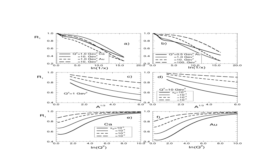
Figure 11: $R_{1}$ as a function of $ln(1/x)$, $lnQ^{2}$ and $A^{1/3}$: a) $R_{1}$ as a function of $ln(1/x)$ for different nucleus and different values of A; b) $R_{1}$ as a function of $lnQ^{2}$ for different values of $x_{B}$ for Au; c) and d) $R_{1}$ as a function of $A^{1/3}$ for different $Q^{2}$; e) and f) $R_{1}$ dependence on $Q^{2}$ for Ca and Au.

Table 1: Values of $R_{1N}$ and $\alpha$ for parameterization $R_{1}\,=\,R_{1N}\,A^{-\,\alpha}$.

	$Q^{2}=1GeV^{2}$		$Q^{2}=10GeV^{2}$
$x$	$R_{1N}$	$\alpha$	$R_{1N}$	$\alpha$
$10^{-2}$	0.94	0.0416	0.98	0.014
$10^{-3}$	0.92	0.0616	0.94	0.034
$10^{-4}$	0.88	0.094	0.92	0.0563
$10^{-5}$	0.8	0.145	0.86	0.093

This picture ( Fig.11 ) shows also that the gluon structure function is far away from the asymptotic one. The asymptotic behavior $R_{1}\,\rightarrow 1$ ( see Figs.11e and f ) occurs only at very high value of $Q^{2}$ as well as in the GLR approach ( see ref. [25] ). The asymptotic $A$-dependence ( $R_{1}\,\propto\,A^{-\frac{1}{3}})$ ) has not been seen in the accessible kinematic range of $Q^{2}$ and $x$ ( see Figs. 11c and d and Table 1 ). This result also has been predicted in the GLR approach [24]. We want also to mention that parameterization $R_{1}\,=\,R_{1N}\,A^{-\alpha}$ does not fit the result of calculations quite well for $1Gev^{2}\,\leq\,Q^{2}\,\leq\,20GeV^{2}$ and $10^{-2}\,\leq\,x\,\leq\,10^{-5}$. For $x\,\sim\,10^{-2}$ the parameterization $R_{1}\,=\,R_{1N}\,-\,R^{\prime}\,A^{\frac{1}{3}}$ with parameters $R_{1N}$ and $R^{\prime}$ for each value of $Q^{2}$, works much better reflecting that only the first correction to the Born term is essential in the Mueller formula.

We extend also the calculation of the exponents $<\omega>$ and $<\gamma>$ of the semiclassical approach for the nuclear case. We calculate the effective power of the nuclear gluon distribution $<\omega>$ using the expression

$$<\omega>\,\,=\,\,\frac{\partial\ln(xG^{A}(x,Q^{2}))}{\partial\ln(1/x)}\,\,.$$ (30)

Fig.12 shows the results as functions of $ln(1/x)$ for different values of $Q^{2}$ and different nucleus. The SC decreases the effective power of the nuclear distribution, giving rise to a flattening of the distribution in the small $x$ region.

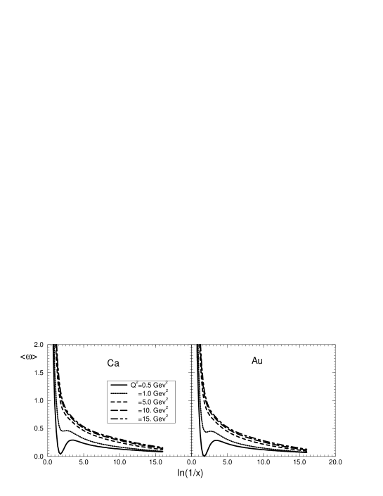
Figure 12: $<\omega>$ for different values of $Q^{2}$ and $A$.

It is also interesting to notice that at small values of $Q^{2}$, the effective power tends to be rather small, even in the nucleon case, at very small $x$. However it should be stressed that the effective power remains bigger than the intercept of the so called ”soft” Pomeron [21], even in the case of a sufficiently heavy nucleus (Au), for $Q^{2}\,>\,1GeV^{2}$. Nowadays, many parameterizations [22] with matching of ”soft” and ”hard” Pomeron have appeared triggered by new HERA data on diffraction dissociation [26]. These parameterization used Pomeron-like behavior namely, $xG(x,Q^{2})\propto x^{-\omega(Q^{2})}$. However, if the Pomeron is a Regge pole, $\omega$ cannot depend on $Q^{2}$, and the only reasonable explanation is to describe $\omega(Q^{2})$ as the result of the SC. Looking at Fig.12 we can claim the SC from the MF cannot provide sufficiently strong SC to reduce the value of $\omega$ to $0.08$, a typical value for the soft Pomeron [21], at least for $Q^{2}\geq 1GeV^{2}$.

The calculation of the effective value of the anomalous dimension $\gamma$ may help us to estimate what distances work in the SC corrections. This effective exponent is given by

$$<\gamma>\,\,=\,\,\frac{\partial\ln(xG^{A}(x,Q^{2}))}{\partial\ln(Q^{2}/Q^{2}_{0})}\,\,.$$ (31)

Figure 13: $<\gamma>$ for different $Q^{2}$ and $A$.

Fig.13 shows the results as functions of $ln(1/x)$ for different values of $Q^{2}$ and for two nuclei. We see that the values of $\gamma$ at $ln(1/x)\,\leq\,5$, for both Ca and Au, is very close to the results for GRV and for nucleon case. At smaller values of $x$, the anomalous dimension presents a sizeable reduction, which increases with A. For $ln(1/x)\,>\,15$, $<\gamma>$ tends to zero unlike in the DGLAP evolution equations ( see Fig.10 for the GRV parameterization). Analysing the $Q^{2}$ dependence, we see that $<\gamma>$ is bigger than $1$ only for $Q^{2}=0.5\,GeV^{2}$. For $Q^{2}=1.0\,GeV^{2}$, the anomalous dimension is close to $1/2$, and for $Q^{2}>5.0\,GeV^{2}$ it is always smaller than $1/2$.

Using semiclassical approach, we see that

$$\kappa\propto\frac{1}{Q^{2}}(Q^{2})^{\gamma}\,,$$ (32)

and if $\gamma\geq 1$, the integral over $r_{t}$ in the master equation (23) becomes divergent, concentrating at small distances.

If $1\,>\,\gamma\geq 1/2$, only the first SC term, namely, the second term in expansion of the master equation, is concentrated at small distances, while higher order SC are still sensitive to small $r_{\perp}$ behavior. Fig.13 shows that this situation occurs for $Q^{2}\,>\,1\,GeV^{2}$, and even for $Q^{2}=1GeV^{2}$ at very small values of $x$. We will return to discussion of these properties of the anomalous dimension behavior in the next section.

3.7 The gluon life time cutoff.

In the DIS the incident electron penetrates the nucleus and radiates the virtual photon whose lifetime $\tau_{\gamma^{*}}\,\propto\,\frac{1}{mx}$ [27]. We can recover three different kinematic regions:

1. $\tau_{\gamma^{*}}\,=\,\frac{1}{mx}\,\,<\,\,R_{NN}$, where $R_{NN}$ is the characteristic distances between the nucleons of the nucleus. This virtual photon can be absorbed only by one nucleon and the total cross section is $\sigma(\gamma^{*}A)\,=\,A\,\sigma(\gamma^{*}p)$.

2. $R_{A}\,\,>\,\,\tau_{\gamma^{*}}\,=\,\frac{1}{mx}\,\,>\,\,R_{NN}$, where $R_{A}$ is the nucleus radius. In this kinematic region the virtual photon can interact with the group of nucleons. However, $\sigma(\gamma^{*}A)$ is still proportional to $A$ since the number of nucleons in a group is much less than $A$.

3. $\tau_{\gamma^{*}}\,=\,\frac{1}{mx}\,\,>\,\,R_{A}$. Here, before reaching the front surface of the nucleus, the virtual photon “decomposes” in the developed parton cascade which then interacts with the nucleus. It can be shown [28] that the absorption cross section of the virtual photon will now be proportional to the surface area of the nucleus $\sigma(\gamma^{*}A)\,\propto\,A^{\frac{2}{3}}$, because the wee partons of the parton cascade are absorbed at the surface and do not penetrate into the centre of the nucleus.

Everything that we have discussed have been calculated in the third kinematic region. For the RHIC energies we have to develop some technique how to penetrate into the second one. To do this we have to remember that the opacity ( or $\kappa_{G}$ ) actually depends on the longitudinal part of the momentum transfer ( $q_{z}$ ) which could be calculated in terms of $x$ and $x^{\prime}$ of our master equation (12) , namely, $q_{z}\,=\,(x+x^{\prime})m$ ( see Ref.[1] ). Recalling that opacity $\Omega\,\propto\,r^{2}_{\perp}xG(x,q_{z},\frac{1}{r^{2}_{\perp}})\,\,S(b_{t},q_{z})$ we see that $q_{z}$ - dependence enters to two factors: to gluon structure function and to the nucleon profile function. We know how to take into account the $q_{z}$ - dependence of the gluon structure function ( see Ref. [2] where the DGLAP equation for $q_{z}\,\neq\,0$ is written ). However we neglected this effect in our present estimates, hoping that this dependence occurs on the hadron scale and cannot change too much the dependence of the SC on the number of collisions during the passage through the nucleus.

The dependence of the profile function $S(b_{t},q_{z})$ on $q_{z}$ have been discussed and in the Gaussian parametrization it can be factor out in the form:

$$S(b_{t},q_{z})\,\,=\,\,S(b_{t})\,\cdot\,L(q_{z})\,\,=\,\,S(b_{t})\,\cdot\,e^{-\,\frac{R^{2}_{A}}{4}\,q^{2}_{z}}\,\,.$$ (33)

This $q_{z}$ - dependence takes into account the fact that the virtual gluon can interact with the target only during the finite time $\tau\,=\,1/mx$ undergoing $\rho\,\tau\,<\,\rho\,R_{A}$ collisions. Using eq. (33), we can obtain:

$$x\,G_{A}(x,Q^{2})\,\,=\,\,A\,x\,G_{N}(x,Q^{2})\,\,-\,\,A\,\frac{\alpha_{\rm S}\,N_{c}}{\pi}\int^{1}_{x}\,\,\int\,\frac{dx^{\prime}}{x^{\prime}}\,\frac{dQ^{\prime 2}}{Q^{\prime 2}}\,\,L(q_{z})\,\,x^{\prime}\,G_{N}(x^{\prime},Q^{\prime 2})$$ (34)

$$+\,\,\frac{2R^{2}_{A}}{\pi^{2}}\,\int^{1}_{x}\,\frac{dx^{\prime}}{x^{\prime}}\,\int^{\frac{1}{Q^{2}_{0}}}_{\frac{1}{Q^{2}}}\,\frac{dr^{2}_{t}}{r^{4}_{t}}\,\,\{\,C\,+\,\ln(L(q_{z})\,\kappa_{G}(x^{\prime},r^{2}_{t}))+\,\,E_{1}(L(q_{z})\,\kappa_{G}(x^{\prime},r^{2}_{t})\,)\}\,\,.$$

Fig. 14 shows the result of our calculations. Comparing Fig.11 with this picture, one can see that the finite life time of the virtual gluon affects the behavior of the gluon structure function only at sufficiently large $x$ ( $x\,\geq\,10^{-2}$ ) diminishing the value of the SC in this kinematic region. This effect turns out to be very important for the RHIC energies and has to be studied in more details.

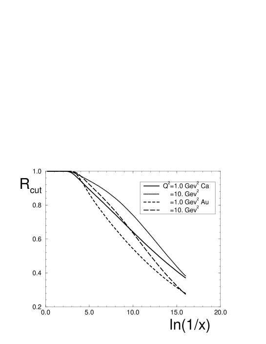
Figure 14: $R_{1}$ for CA and Au with gluon life time cutoff.

4 First corrections to the Glauber ( Mueller) Approach.

In this section we discuss the corrections to the Glauber approach (the Mueller formula of eq. (12) . To understand how big could be the corrections to the Glauber approach we calculate the second iteration of the Mueller formula of eq. (12). As has been discussed,eq. (12) describes the rescattering of the fastest gluon ( gluon - gluon pair ) during the passage through a nucleus ( see Fig.1 ). In the second iteration we take into account also the rescattering of the next to the fastest gluon. This is a well defined task due to the strong ordering in the parton fractions of energy in the parton cascade in leading $ln(1/x)$ approximation of pQCD that we are dealing with. Namely:

$$x_{B}\,\,<\,\,x_{n}\,\,<\,\,...\,\,<x_{1}\,\,<\,\,1\,\,;$$ (35)

where 1 corresponds to the fastest parton in the cascade.

Therefore, in the second interaction we include the rescatterings of the gluons with the energy fraction $1$ and $x_{1}$ ( see Fig.15 ). Doing the first iteration we insert in eq. (12) $G_{N}(x,Q^{2})\,=\,G^{GRV}_{N}(x,Q^{2})$. For the second iteration we calculate the gluon structure function using eq. (12) substituting

$$x\,G_{N}\,\,=\,\,\frac{xG^{1}_{A}(x,Q^{2})}{A}\,\,-\,\,x\,G^{GRV}_{N}(x,Q^{2})\,\,;$$ (36)

where $xG^{1}_{A}$ is the result of the first iteration of eq. (12) that has been discussed in details in section 3.

Figure 15: The interaction with nucleons that is taken into account in the second iteration of M ueller formula.

Fig.16 shows the need to subtract $xG^{GRV}_{N}$ in eq. (36) making the second iteration. Indeed, in the second iteration we take into account the rescattering of gluon $1^{\prime}$ - gluon $2^{\prime}$ pair off a nucleus. We picture in Fig.16 the first term of such iteration in which $G_{1^{\prime}}G_{2^{\prime}}$ pair has no rescatterings. It is obvious that it has been taken into account in our first iteration, so we have to subtract it to avoid a double counting.

Figure 16: The first term of the second iteration of eq. (36).

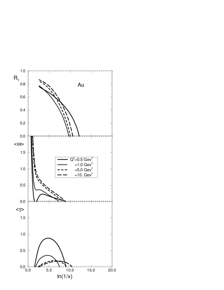
Figure 17: Second iteration calculations for $R_{1}$, $<\omega>$, and $<\gamma>$ for Ca and Au.

One can see in Figs.17 that the second iteration gives a big effect and changes crucially $R_{1}$, $<\gamma>$, and $<\omega>$. The most remarkable feature is the crucial change of the value of the effective power $\omega(Q^{2})$ for the “Pomeron” intercept which tends to zero at HERA kinematic region, making possible the matching with “soft” high energy phenomenology. It is also very instructive to see how the second iteration makes more pronounced all properties of the behavior of the anomalous dimension ( $<\gamma>$) that we have discussed. The main conclusions which we can make from Figs.17 are: (i) the second iteration gives a sizable contribution in the region $x\,\,<\,\,10^{-2}$ and for $x\,\,\leq\,\,10^{-3}$ it becomes of the order of the first iteration; (ii) for $x\,\,<\,\,10^{-3}$ we have to calculate the next iteration. It means that for such small $x$ we have to develop a different technique to take into account rescatterings of all the partons in the parton cascade which will be more efficient than the simple iteration procedure for eq. (12). However, let us first understand why the second iteration becomes essential to establish small parameters that enter to our problem.

As has been discussed, we use the GLAP evolution equations for gluon structure function in the region of small $x$. It means, that we sum the Feynman diagrams in pQCD using the following set of parameters:

$$\alpha_{\rm S}\,\,\ll\,\,1\,\,;\,\,\,\,\,\,\,\,\,\,\alpha_{\rm S}\,\ln\frac{1}{x}\,\,<\,\,1\,\,;\,\,\,\,\,\,\,\,\,\,\alpha_{\rm S}\,\ln\frac{Q^{2}}{Q^{2}_{0}}\,\,<\,\,1\,\,;\,\,\,\,\,\,\,\,\,\,\alpha_{\rm S}\,\,\ln\frac{Q^{2}}{Q^{2}_{0}}\,\,\ln\frac{1}{x}\,\,\approx\,\,1\,\,.$$ (37)

The idea of the theoretical approach of rescattering that has been formulated in the GLR paper [2] is to introduce a new parameter :

$$\kappa\,\,=\,\,\frac{N_{c}\,\alpha_{\rm S}\,\pi\,A}{2\,Q^{2}\,R^{2}_{A}}\,xG(x,Q^{2})$$ (38)

and sum all Feynman diagrams using the set of eq. (37) and $\kappa$ as parameters of the problem, neglecting all contributions of the order of: $\alpha_{\rm S}$, $\alpha_{\rm S}\,\kappa$, $\alpha_{\rm S}\ln(1/x)$, $\alpha_{\rm S}\ln(1/x)\,\kappa$, $\alpha_{\rm S}\ln(Q^{2}/Q^{2}_{0})$ and $\alpha_{\rm S}\ln(Q^{2}/Q^{2}_{0})\,\kappa$. It should be stressed that Mueller formula gives a solution for such approach. Indeed, eq. (12) depends only on $\kappa$ absorbing all
$(\,\alpha_{\rm S}\,\ln(Q^{2}/Q^{2}_{0})\,\ln(1/x)\,)^{n}$ contributions in $xG(x,Q^{2})$. However, it is not a complete solution. To illustrate this point let us compare the value of the second term of the expansion of eq. (12) with respect to $\sigma(r^{2}_{t})$ with the first correction due to the second iteration in the first term of such an expansion. In other words we wish to compare the values of the diagrams in Fig.18 b and Fig.18a. The contribution of the diagram of Fig.18a is equal:

$$\Delta xG(x,Q^{2})\,(\,Fig.\ref{fig.18}a\,)\,\,=\,\,\frac{R^{2}_{A}}{2\,\pi^{2}}\,\,\int\frac{dx^{\prime}}{x^{\prime}}\,\int\,dQ^{\prime 2}\,\,\kappa^{2}(x^{\prime},\frac{Q^{\prime 2}}{4})\,\,,$$ (39)

where $x^{\prime}$ and $Q^{\prime 2}$ are the fraction of energy and the virtuality of gluon $1$ in Fig.18a

The diagram of Fig.18b contains one more gluon and its contribution is:

$$\Delta xG(x,Q^{2})\,(\,Fig.\ref{fig.18}b\,)\,\,=\,\,\frac{R^{2}_{A}}{\pi^{2}2}\,\,\frac{N_{c}\alpha_{\rm S}}{\pi}\int\,\,\frac{dx^{\prime}}{x^{\prime}}\,\,\frac{dQ^{\prime 2}}{Q^{\prime 2}}\,\,\int\frac{dx"}{x"}\,\int\,dQ"^{2}\,\,\kappa^{2}(x",\frac{Q"^{2}}{4})$$

$$\propto\,\,\frac{\alpha_{\rm S}N_{c}}{\pi}\,\,\ln(1/x)\,\,\ln(Q^{2}/Q^{2}_{0})\,\,\Delta xG(x,Q^{2})(\,Fig.\ref{fig.18}a)\,)\,\,,$$ (40)

where $x^{\prime}$ ($x^{\prime\prime}$) and $Q^{\prime 2}$ ( $Q^{\prime\prime 2}$) are the fraction of energy and the virtuality of gluon $1$ ($1^{\prime}$) respectively in Fig.18b.

Figure 18: Corrections to the Glauber approach.

Therefore, eq. (40) gives the contribution which is of the order of eq. (39) in the kinematic region where the set of parameters of eq. (37) holds. It means also that we need to sum all diagrams of Fig.18b type to obtain the full answer. In the diagram of Fig.18b not only one but many gluons can be emitted. Such emission leads to so called “triple ladder” interaction, pictured in Fig.18c ( see ref.[2] ). This diagram is the first from so called “fan” diagrams of Fig. 18d. To sum them all we can neglect the third term in eq. (12) and treat the remained terms as an equation for $xG(x,Q^{2})$. It is easy to recognize that we obtain the GLR equation [2][10]. Generally speaking the GLR equation sums the most important diagrams in the kinematic region where $\alpha_{\rm S}\,\ln(1/x)\,\ln(Q^{2}/Q^{2}_{0})\,\,\gg\,\,1$ and $\kappa\,<\,1$.

5 The general approach.

5.1 Why equation?

We would like to suggest a new approach based on the new evolution equation to sum all SC. However, first of all we want to argue why an equation is better than any iteration procedure. To illustrate this point of view let us differentiate the Mueller formula with respect to $y\,=\,\ln(1/x)$ and $\xi\,=\,\ln Q^{2}$. It is easy to see that this derivative is equal to

$$\frac{\partial^{2}xG(x,Q^{2})}{\partial y\,\partial\xi}\,\,=\,\,\frac{4}{\pi^{2}}\,\int db^{2}_{t}\,\,\{\,\,1\,\,-\,\,e^{-\,\frac{1}{2}\,\sigma(x,r^{2}_{\perp}\,=\,\frac{1}{Q^{2}})\,S(b^{2}_{t})}\,\,\}\,\,.$$ (41)

The nice property of eq. (41) is that everything enters at small distances, therefore everything is under theoretical control. Of course, we cannot get rid of our problems changing the procedure of solution. Indeed, the nonperturbative effects coming from the large distances are still important but they are all hidden in the boundary and initial conditions to the equation. Therefore, an equation is a good ( correct ) way to separate what we know ( small distance contribution) from what we don’t ( large distance contribution).

5.2 The generalized evolution equation.

We suggest the following way to take into account the interaction of all partons in a parton cascade with the target. Let us differentiate the Mueller formula over $y\,=\,\ln(1/x)$ and $\xi=\ln(Q^{2}/Q^{2}_{0})$. It gives:

$$\frac{\partial^{2}xG_{A}(y,\xi)}{\partial y\partial\xi}\,\,=\,\,\frac{2\,R^{2}_{A}\,\,Q^{2}}{\pi^{2}}\,\,\{\,\,C\,\,+\,\,\ln\kappa\,\,+\,\,E_{1}(\kappa)\,\,\}\,\,.$$ (42)

Rewriting eq. (42) in terms of $\kappa$ given by

$$\kappa\,\,=\,\,\frac{N_{c}\alpha_{\rm S}\pi}{2Q^{2}R^{2}_{A}}\,xG_{A}(x,Q^{2})$$ (43)

we obtain:

$$\frac{\partial^{2}\kappa(y,\xi)}{\partial y\partial\xi}\,\,+\,\,\frac{\partial\kappa(y,\xi)}{\partial y}\,\,=\,\,\frac{N_{c}\,\alpha_{\rm S}\,}{\pi}\,\,\{\,\,C\,\,+\,\,\ln\kappa(y,\xi)\,\,+\,\,E_{1}(\kappa(y,\xi))\,\,\}\,\,\equiv\,\,F(\kappa)\,\,.$$ (44)

Now, let us consider the expression of eq. (44) as the equation for $\kappa$ This equation has the following nice properties:

1. It sums all contributions of the order $(\,\alpha_{\rm S}\,y\,\xi\,)^{n}$ absorbing them in $xG_{A}(y,\xi)$, as well as all contributions of the order of $\kappa^{n}$. Therefore, this equation solves the old problem, formulated in Ref.[2] and for $N_{c}\,\rightarrow\,\infty$ eq. (44) gives the complete solution to our problem, summing all SC;

2 .The solution of this equation matches with the solution of the DGLAP evolution equation in the DLA of perturbative QCD at $\kappa\,\rightarrow\,0$;

3. At small values of $\kappa$ ( $\kappa\,<\,1$ ) eq. (44) gives the GLR equation. Indeed, for small $\kappa$ we can expand the r.h.s of eq. (44) keeping only the second term. Rewriting the equation through the gluon structure function we have

$$\frac{\partial^{2}xG_{A}(y,\xi)}{\partial y\partial\xi}\,\,=\,\,\frac{\alpha_{\rm S}N_{c}}{\pi}\,xG(x,Q^{2})\,\,-\,\,\frac{\alpha_{\rm S}A^{2}}{2R^{2}_{A}}\,(xG(x,Q^{2}))^{2}\,\,,$$ (45)

which is the GLR equation [2] with the coefficient in front of the second term calculated by Mueller and Qiu [10].

4. For $\alpha_{\rm S}y\xi\,\approx\,1$ this equation gives the Glauber ( Mueller ) formula, that we have discussed in details.

5. This equation almost coincide with the equation that L.Mclerran with collaborators [29] derived from quite different approach and with different technique. We are sure that almost will disappear when they will do more careful averaging over transverse distances.

Therefore, the great advantage of this equation in comparison with the GLR one is the fact that it describes the region of large $\kappa$ and provides the correct matching both with the GLR equation and with the Glauber ( Mueller ) formula.

Eq. (44) is the second order differential equation in partial derivatives and we need two initial ( boundary ) conditions to specify the solution. The first one is obvious, namely, at fixed $y$ and $Q^{2}\,\rightarrow\,\infty$

$$\kappa\,\,\rightarrow\,\,\frac{N_{c}\,\alpha_{\rm S}\,\pi\,A}{2\,Q^{2}\,R^{2}_{A}}\,xG^{GLAP}_{N}(x,Q^{2})\,\,.$$

The second one we can fix in the following way: at $x=x_{0}\,\,(y=y_{0})$ which is small, namely, in the kinematic region where $\alpha_{\rm S}y\xi\,\leq\,1$

$$\kappa\,\,\rightarrow\,\,\kappa_{in}\,\,=\,\,\frac{N_{c}\,\alpha_{\rm S}\,\pi}{2\,Q^{2}\,R^{2}_{A}}\,xG_{A}(x,Q^{2})\,\,,$$ (46)

where $xG_{A}$ is given by the Mueller formula ( see eq. (12)). Practically, we can take $x_{0}\,=\,10^{-2}$, because corrections to the MF are small at this value of $x=x_{0}$.

5.3 The asymptotic solution.

First observation is the fact that eq. (44) has a solution which depends only on $y$. Indeed, one can check that $\kappa\,=\,\kappa_{asymp}(y)$ is the solution of the following equation:

$$\frac{d\kappa_{asymp}}{dy}\,\,=\,\,F(\,\kappa_{asymp}\,)\,\,.$$ (47)

The solution to the above equation is:

$$\int^{\kappa_{asymp}(y)}_{\kappa_{asymp}(y=y_{0})}\,\,\frac{d\kappa^{\prime}}{F(\kappa^{\prime})}\,\,=\,\,y-y_{0}\,\,.$$ (48)

It is easy to find the behavior of the solution to eq. (48) at large value of $y$ since $F(\kappa)\,\,\rightarrow\,\,\bar{\alpha}_{\rm S}\ln\kappa$ at large $\kappa$ ( $\bar{\alpha}_{\rm S}=\frac{N_{c}}{\pi}\,\alpha_{\rm S}$ ). It gives

$$\kappa_{asymp}\,\,\rightarrow\,\,\bar{\alpha}_{\rm S}y\,\ln(\bar{\alpha}_{\rm S}y)\,\,\,\,\,\,at\,\,\,\,\,\,\,\bar{\alpha}_{\rm S}y\,\,\gg\,\,1\,\,.$$ (49)

At small value of $y$, $F(\kappa)\,\,\rightarrow\,\,\bar{\alpha}_{\rm S}\kappa$ and we have:

$$\kappa_{asymp}\,\,\rightarrow\,\,\kappa_{asymp}(y=y_{0})\,\,e^{\bar{\alpha}_{\rm S}(y-y_{0})}\,\,.$$ (50)

The solution is given in Fig.19 for $\bar{\alpha}_{\rm S}=1/4$ in the whole region of $y$ for different nuclei in comparison with our calculations based on the MF. We chose the value of $\kappa_{asymp}(y=y_{0})$ from eq. (46). We claim this solution is the asymptotic solution to eq. (44) and will argue on this point a bit later.

For nuclei the SC incorporated in the asymptotic solution turn out to be much stronger than the SC in the Glauber approach for any $Q^{2}\,>\,1\,GeV^{2}$ at $x\,>\,10^{-2}$. In this kinematic region the solution of eq. (44) is drastically different from the Glauber one.

A general conclusion for Fig.19 is very simple: the amount of shadowing which was taken into account in the MF is not enough , at least for the gluon structure function in nuclei at $x\,<\,10^{-2}$ and we have to solve eq. (44) to obtain the correct behavior of the gluon structure function for nuclei.

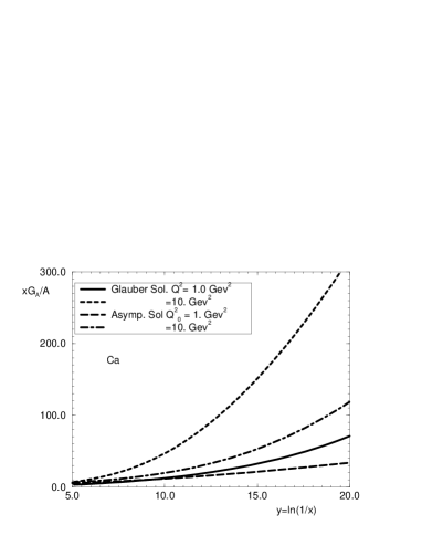
Figure 19: The Glauber approach and asymptotic solution for different nuclei.

Now, we would like to show that solution eq. (44) is the asymptotic solution of the new evolution equation. In order to check this we need to prove that this solution is stable. It means that if add a small function $\Delta\kappa$ and searching for the solution to the equation in the form $\kappa\,=\,\kappa_{asymp}\,+\,\Delta\kappa$, we have to prove that $\Delta\kappa$ turns out to be small.namely, $\Delta\kappa\,\ll\,\kappa$. The following linear equation can be written for $\Delta\kappa$:

$$\frac{\partial^{2}\Delta\kappa(y,\xi)}{\partial y\,\partial\xi}\,\,+\,\,\frac{\partial\Delta\kappa(y,\xi}{\partial y}\,\,=\,\,\frac{dF(\kappa)}{d\kappa}\,|_{\kappa=\kappa_{asymp}(y)}\,\,\Delta\kappa(y,\xi)\,\,.$$ (51)

In Ref.[1] was proven, that the solution of eq. (51) is much smaller than $\kappa$.

Therefore the asymptotic solution has a chance to be the solution of our equation in the region of very small $x$. To prove that the asymptotic solution is the solution to the equation we need to solve our equation in the wide kinematic region starting with our initial condition. We managed to do this only in semiclassical approach.

5.4 Semiclassical Approach.

The semiclassical approach has been adjusted to the solution of the nonlinear equation of eq.(44)-type in Refs. [2, 30, 31] ( for simplicity, we assume that $\alpha_{\rm S}$ is fixed ).

In the semiclassical approach we are looking for the solution of eq. (44) in the form

$$\kappa=e^{S}$$ (52)

where $S$ is a function with partial derivatives: $\frac{\partial S}{\partial y}=\omega$ and $\frac{\partial S}{\partial\xi}=\gamma$ which are smooth function of $y$ and $\xi$. It means that

$$\frac{\partial^{2}S}{\partial\xi\partial y}\ll\frac{\partial S}{\partial y}\cdot\frac{\partial S}{\partial\xi}=\omega\gamma$$ (53)

Using eq.(53), one can easily rewrite eq.(44) in the form

$$\frac{\partial S}{\partial y}\frac{\partial S}{\partial\xi}+\frac{\partial S}{\partial y}=e^{-S}F(e^{S})\equiv\Phi(S)$$ (54)

or

$$\omega(\gamma+1)=\Phi(S)$$ (55)

We are going to use the method of characteristics( see, for example, ref.[33]). For equation in the form

$$F(\xi,y,S,\gamma,\omega)=0$$ (56)

we can introduce the set of characteristic lines $(\xi(y),S(y),\omega(y),\gamma(y))$, which satisfy a set of well defined equations (see, for example, Refs. [30] [31] for the method and Ref [1] for detailed calculation). Using eq.(54) and eq.(55), we obtain the following set of equations for the characteristics:

$$\frac{d\xi}{dy}=\frac{\Phi(S)}{(\gamma+1)^{2}}\,;\,\,\,\,\,\frac{dS}{dy}=\frac{2\gamma+1}{(\gamma+1)^{2}}\Phi(S)\,;\,\,\,\,\frac{d\gamma}{dy}=\Phi^{\prime}_{S}\frac{\gamma}{\gamma+1}\,\,,$$ (57)

where $\Phi^{\prime}_{S}\,=\,\frac{\partial\Phi}{\partial S}$. The initial condition for this set of equations we derive from eq.(46), namely

$$S_{0}=ln\kappa_{in}(y_{0},\xi_{0})$$

$$\gamma_{0}=\left.\frac{\partial ln\kappa_{in}(y_{0},\xi)}{\partial\xi}\right|_{\xi=\xi_{0}}$$ (58)

The main properties of these equations have been considered in Ref.[1] analytically, however, here, we restrict ourselves mostly the numeric solution of these equations.

We set the initial condition $y=y_{0}=4.6$ ($x_{B}=10^{-2}$), where the shadowing correction is not big and the evolution starts from $\gamma<0$. In this case $d\gamma/dy>0$ and the value of $\gamma$ increases . At the same time $dS/dy<0$ and $S$ decreases if $\gamma_{0}<-1/2$. With the decrease of $S$, the value of $\Phi^{\prime}_{S}$ becomes smaller and after short evolution the trajectories of the nonlinear equation start to approach the trajectories of the DGLAP equations. We face this situation for any trajectory with $\gamma_{0}$ close to -1. If the value of $\gamma_{0}$ is smaller than $-\,\frac{1}{2}$ but the value of $S_{0}$ is sufficiently big, the decrease of $S$ due to evolution cannot provide a small value for $\Phi^{\prime}(S)$ and $\gamma$ increases until its value becomes bigger than $-\frac{1}{2}$ at some value of $y=y_{c}$. In this case for $y>y_{c}$ the trajectories behave as in the case with $\gamma_{0}\,>\,-\,\frac{1}{2}$. For $\gamma_{0}>-1/2$, the picture changes crucially. In this case, $dS/dy>0$ , $d\gamma/dy>0$ and both increase. Such trajectories go apart from the trajectories of the DGLAP equation and nonlinear effects play more and more important role with increasing $y$. These trajectories approach the asymptotic solution very quickly.

For the numerical solution we use the 4th order Runge - Kutta method to solve our set of equations with the initial distributions of eq. (58). The result of the solution is given in Figs.20 and 21. In these figures we plot the bunch of the trajectories with different initial conditions. For the nucleon ( Fig.20 ) we show also the dependence of $\gamma$ along these trajectories. One can notice that the trajectories behave in the way which we have discussed in our qualitative analysis. It is interesting to notice that the trajectories, which are different from the trajectories of the GLAP evolution equations, start at $y=y_{0}=4.6$ with the values of $Q^{2}$ between $0.5GeV^{2}$ and $2.5GeV^{2}$ for a nucleon. It means that, guessing which is the boundary condition at $Q^{2}=Q^{2}_{0}=2.5GeV^{2}$, we can hope that the linear evolution equations ( the DGLAP equations) will describe the evolution of the deep inelastic structure function in the limited but sufficiently wide range of $Q^{2}$.

In Figs. 20 and 21 we plot also the lines with definite value of the ratio $R\,=\,\frac{xG(x,Q^{2})(generalized\,\,\,equation)}{xG(x,Q^{2})(GLAP)}$ (horizontal lines). These lines give the way to estimate how big are the SC. One can see that they are rather big.

Figure 20: The trajectories and contour plot for the solution of the generalized evolution equation for N.   $R\,=\,\frac{xG(x,Q^{2})(generalized\,\,\,equation)}{xG(x,Q^{2})(GLAP)}$.

Figure 21: The trajectories and contour plot for the solution of the generalized evolution equation for Ca and Au.   $R\,=\,\frac{xG(x,Q^{2})(generalized\,\,\,equation)}{xG(x,Q^{2})(GLAP)}$.

We have discussed only the solution with fixed coupling constant which we put equal to $\alpha_{\rm S}=0.25$ in the numerical calculation. The problem how to solve the equation with running coupling constant is still open.

5.5 The generalized evolution equation versus the GLR equation.

In Ref.[1] we studied in detail the solution to the GLR equation in the same semiclassical approximation. Our conclusion is that the GLR equation gives much stronger SC than the generalized evolution equation. This difference we can see comparing the solution to the both equation in the region ultra small $x$.

Indeed, our asymptotic solution turns out to be quite different from the GLR one. The GLR solution in the region of very small $x$ leads to saturation of the gluon density [30, 31, 32]. Saturation means that $\kappa$ tends to a constant in the region of small $x$. The solutions of eq. (44) approach the asymptotic solution at $x\,\rightarrow\,0$, which does not depend on $Q^{2}$, but exhibits sufficiently strong dependence of $\kappa$ on $x$ ( see Fig.19 ), namely $\kappa\,\propto\,\alpha_{\rm S}\ln(1/x)\ln\ln(1/x)$. The absence of saturation does not contradict any physics since gluons are bosons and it is possible to have a lot of bosons in the same cell of the phase space. We should admit that A. Mueller first came to the same conclusion using his formula in Ref.[3].

6 Next steps.

Here, we list our problems that have to be solved to complete our study of the SC :

1. Calculation of $F^{A}_{2}(x,Q^{2})$ to compare our calculation of the SC with the available experimental data.

2. Recalculation of the SC using more reliable Wood-Saxon parameterization for profile function $S(b_{t})$ instead of the Gaussian one. The form of the profile function especially essential to obtain a reliable estimates for the SC in the region of the moderate $x\,\leq\,\frac{1}{2mR_{A}}$.

3. Solution of the generalized evolution equation for running $\alpha_{\rm S}$. The experience of solving the GLR equation tells us that there is a principal difference in the solutions for fixed and running $\alpha_{\rm S}$, namely, the critical line of the GRL equation appears only for running $\alpha_{\rm S}$ [2]. We think that it is very important to study the generalized equation with running $\alpha_{\rm S}$ and to compare this solution with the solution of the GRL equation.

4. We have discussed that for RHIC energies it is very important to study in more details the effect of the final life-time of th gluon in a nucleus. We plan to recalculate the SC replacing $xG(x,Q^{2})$ in our formulae by $xG(x,Q^{2},q_{z})$ for which the kernels of the evolution equations have been calculated in Ref.[2].

5. In all our calculations we neglected the parton interaction inside $GG+N$ scattering. Our estimates, which have been presented in section 2, shows that this interaction should be very important. Indeed, for example, in the Mueller formula we have to change the parameter $\kappa_{G}$ due to the parton interaction inside the nucleon. This change is simple, the only that we need to do is to replace the number of collisions $A/\pi R^{2}_{A}$ by

$$\frac{A}{\pi R^{2}_{A}}\,\,\rightarrow\,\,\frac{A}{\pi R^{2}_{A}}\,\,+\,\,\frac{1}{\pi R^{2}_{N}}$$

in the definition of $\kappa_{G}$ in eq. (12). It means that all results will be the same but nucleus with the new effective number of nucleons:

$$A^{\frac{1}{3}}_{eff}\,\,=\,\,A^{\frac{1}{3}}\,\,+\,\,\frac{R^{2}_{0}}{R^{2}_{N}}\,\,,$$

where $R_{A}=R_{0}\,A^{\frac{1}{3}}$. Using our estimates for $R^{2}_{N}=5GeV^{-2}$ we can see that effective A for the gold is $A^{\frac{1}{3}}_{eff}\,\,=9.6$ instead $A^{\frac{1}{3}}\,=\,6$. For light nuclei the change is even more essential. Therefore, we are planning to take into account the parton interaction inside a nucleon as soon as possible.

6. We have neglected all correlations between partons of the order $\frac{1}{N^{2}_{c}}$ which could be sizable in the case of the nucleus DIS. We suppose to study this problem using the technique that has been developed in Ref.[34].

7. Everywhere through the paper we used the DLA of perturbative QCD. However, the key assumption that simplify our theoretical approach was the $\alpha_{\rm S}\ln(1/x)\,\approx\,1$ approximation. We plan to develop our approach in the case of the BFKL dynamic and, therefore, to get rid of our assumption that $\alpha_{\rm S}\ln(Q^{2}/Q^{2}_{0})\,\,\approx\,\,1$. We consider this generalization as an important step, since our result that we have no saturation of the gluon density in nuclei even at ultra small $x$ could be an artifact our double log approximation of perturbative QCD.

7 And what?

We presented here our approach to the SC and a natural question arises:and what? What and how we can do for the RHIC physics. How our approach can help in creating of the reliable Monte Carlo code for nucleus - nucleus interaction at high energies.We are going to answer these hot question in this section.

Let us consider first the space time structure of the nucleus - nucleus interaction ( see Fig.22).

Figure 22: Four stages of nucleus - nucleus collision.

One can see four stages of this process:

1. For time smaller that $t_{0}$, where $t_{0}$ is the time of the first parton - parton interaction, we have a very coherent system of parton, confined in our both nuclei. We know almost nothing about this system.

2. At time $t_{0}$ the first parton - parton interaction occurs and we believe that this interaction destroys the coherence of our parton system at the very instant.

3. During time from $t_{0}$ till $t_{h}$, where $t_{h}$ is the hadronization time, we have a quark - gluon stage of the process. We believe that we can reach a simple and economic understanding this stage in framework of QCD. We also believe that new collective phenomena could be created in the nucleus - nucleus interaction during this stage of the process such as the Quark - Gluon Plasma mostly because of the high density of the produced gluons. For this stage we have the Monte Carlo codes based on QCD, the lattice calculation and a lot of beautiful ideas that has been discuss at this conference.

4. The last stage - hadronization is a black box. Nothing is known, but the success of the Local- Hadron-Parton Duality in the description of the LEP data allows us to hope that this stage could be not very important for our understanding of the nucleus - nucleus collisions.

Our approach can define the initial condition at $t=t_{0}$ for the third stage. What can we do?

1. We are able to calculate the inclusive cross section for gluons at $t=t_{0}$ or, in other words, define the gluon distribution at $t=t_{0}$. Actually, it has been done by C.Escola [35] and his collaborator and has been presented at this conference. We can only improve his treatment of the SC which was based on the GLR equation. However, let us discuss briefly the formula for the inclusive gluon cross section. It can be written using the factorization theorem [36] in the form:

$$\frac{d\sigma}{dy\,dp^{2}_{t}}\,\,=\,\,\propto\,\,\int\,dx_{1}dx_{2}\,x_{1}G_{A_{1}}(x_{1},p^{2}_{t})\,x_{2}G_{A_{2}}(x_{2},p^{2}_{t})\,\,\frac{\alpha_{\rm S}}{p^{4}_{t}}\,\,$$

where the last factor is the hard gluon - gluon cross section and $y$ and $p_{t}$ are rapidity and transverse momentum of produced gluon, respectively. One can see that this cross section is infrared unstable and diverges at small values of $p_{t}$. The SC provides a natural scale that cut off this divergence. A rough estimate for this new scale can be done from equation

$$\kappa_{G}(x,r^{2}_{\perp}=\frac{1}{Q^{2}_{0}(x)})\,\,=\,\,1\,\,$$

(see Fig.4 ). For $p_{t}\,<\,Q_{)}(x)$ the gluon structure function $xG(x,p^{2}_{t})\,\,\propto\,\,p^{2}_{t}$ and one can see that the number of gluon with transverse momenta smaller than $p_{t}=Q_{0}(x)$ turns out to be very small.

2. We can calculate also the double inclusive cross section which gives the two gluon correlation function at $t=t_{0}$. We would like to stress that for nucleus - nucleus collision this correlation function is big and have to be taken into account. Indeed, we have two different contribution to the double inclusive process, pictured in Fig.23: the production of two gluons from one parton cascade (see Fig.23a) and from two parton cascades ( see Fig.23b ). However, for nucleus - nucleus collisions the first contribution is proportional to $A_{1}A_{2}$ ( without the SC) while the second is much bigger and it is of the order of $A^{2}_{1}A^{2}_{2}\,\frac{R^{2}_{A_{1}}\,+\,R^{2}_{A_{2}}}{\pi R^{2}_{A_{1}}R^{2}_{A_{2}}}$ ( without the SC and for the Gaussian profile function). Using our approach we can calculate the two gluon correlation function within better acuraccy than the above simple estimates. We hope, that these two observables: gluon distribution and two gluon correlation function will be enough for reliable description of the initial condition for the QCD motivated cascade during the third stage of our process.

Figure 23: Double inclusive cross section in QCD.

3. We think that these two observables: multiplicity of gluons and two gluon correlation will be enough to define the initial condition for current Monte Carlo codes. However, we think that these codes are doing something wrong. Indeed, we learned from A. Mueller [17] that correct degrees of freedom for parton cascading looks in the simplest way and which could be used for a probabilistic interpretation and therefore, they are natural degrees of freedom for Monte Carlo simulations are not quark and gluons but colourless quark - antiquark dipoles. The gluon structure function is the probability to find a colourless dipole with the size $r_{\perp}\,\geq\,\frac{1}{Q}$. Therefore, we think that the code should be written for such dipoles and their interaction. We shall answer the questions:(i) how to calculated the average multiplicity of dipoles with the size $r_{\perp}$ and (ii) how to calculate the correlations between such dipoles. We are going to do this in the nearest future.

4. Now we want to discuss a hot question how to mix the ”soft” and ”hard” Pomerons. The common way of doing such a mixture is to use the Glauber formula and replace in this formula $\sigma(r^{2}_{\perp}\,\rightarrow\sigma_{soft}\,+\,\sigma_{hard}$. We think this is a correct procedure to obtain an estimate how important soft or/and hard processes. In section 3 we argued that this is the most economic way of doing which satisfies the $s$-channel unitarity. However, all Monte Carlo programs that we know use for the calculation of $\sigma_{hard}$ the factorization formula, namely

$$\sigma_{hard}\,\,=\,\,\frac{!}{2}\,\int_{p^{2}_{0}}\,dp^{2}_{t}\,x_{1}G(x_{2},p^{2}_{t})x_{2}G(x_{2},p^{2}_{t})\,\frac{\alpha_{\rm S}^{2}}{p^{4}_{t}}\,\,,$$

which describes really the inclusive production of gluons. The factor 1/2 in front does not help because to find $\sigma_{hard}$ we need to calculate the real multiplicity but not the number of gluon line in the Feynman diagram. In Fig.24 we picture the $\alpha_{\rm S}^{3}$ corrections to the hard cross section considering the scattering of two mesons made from heavy quarks. Perturbative QCD is certainly a good tool to study such processes. From this picture one sees that including the inclusive cross section in the place of the total we missed the radiative correction to the the partial cross section with four quarks i the final state.

Figure 24: Total cross section in $\alpha_{\rm S}^{2}$ and $\alpha_{\rm S}^{3}$ orders of perturbative QCD.

Our way of doing is the following. We will write the Mueller formula or our more sofisticated approach for dipole (with size $r_{\perp}$ scattering with a nucleus. To find the proton - nucleus cross section we need to calculate the integral:

$$\sigma(pA)\,\,=\,\,\int^{1}_{0}\prod^{3}_{1}dz_{i}\int\prod\frac{d^{2}r^{ik}_{\perp}}{2\pi}\Psi_{p}(z_{i},r^{ik}_{\perp}\,\,2\,\{\,\,1\,\,-\,\,e^{-\,\frac{1}{2}\sigma_{n}(r^{ik}_{\perp}S(b_{t})}\,\,\}\,\,\Psi^{*}(r^{ik}_{\perp},z_{i})\,\,.$$

To find the wave function of the nucleon we have to use a model,for example the constituent quark model or instanton liquid model. The nice feature of this formula that the typical $r^{ik}_{\perp}$ will be of the order 1 $GeV^{-1}$ due to the SC. It means that we need to know the wave function at sufficiently small distances where we have some control from lattice calculations and QCD sum rules. This formula takes into account correctly hard process and give the factorization formula for the inclusive production. We suppose to do an estimates using the model for the nucleon wave function. If they will show that we need some admixture of the soft processes we will add to $\sigma_{N}$ in the above formula in an usual phenomenologic way, using the model of, so called, soft Pomeron.

8 Conclusions.

We have two conclusions:

1. We hope that we convinced you that we are on the way from our Really Highly Inefficient Calculation to your RHIC. Much work is need to clarify the initial condition for the QCD phase of nucleus - nucleus interaction and this is the first and the most important task which we need to attack, since it will determine the correct degrees of freedom for further evolution of QCD cascades.

2. Everything that we have talked about satisfies the third law of theoretical physics:Any model is a theory which we apply to a kinematic region, where we cannot prove that this theory is wrong. We firmly believe that correct SC will provide the picture of the nucleus - nucleus interaction in which hard and semihard processes will play a crucial role with only small if any contamination of the soft contribution.

Acknowledgements:

One of us (E.M.L.) is very grateful to Sid Kahana for creation a stimulating atmosphere of discussion at RHIC’96 Workshop and for enlighting discussions of the difficult theoretical problems in the modeling heavy ion collisions. E.M.L. thanks all participant of the hard working group and especially Yu. Dokshitzer,C.Eskola, A. Mueller and M.Strikman for fruitful discussions on the subject of the talk and related topics. MBGD thanks A. Capella and D.Schiff for enlightening discussions. Work partially financed by CNPq, CAPES and FINEP, Brazil.

References

- [1] A.L.Ayala,M.B.Gay Ducati and E.M. Levin: CBPF-FN-020/96,hep-ph 9604383.
- [2] L. V. Gribov, E. M. Levin and M. G. Ryskin: Phys.Rep. 100 (1983) 1.
- [3] A.H. Mueller: Nucl. Phys. B335 (1990) 115;
-
[4]
H1 collaboration,T. Ahmed et al.: Nucl. Phys. B439 (1995) 471;
ZEUS collaboration, M. Derrick et al.: Z. Phys. C 69 (1995) 607; H1 collaboratrion, S. Aid et al.: DESY 96 - 039 (1996). - [5] V.N. Gribov and L.N. Lipatov: Sov. J. Nucl. Phys. 15 (1972) 438; L.N. Lipatov: Yad. Fiz. 20 (1974) 181; G. Altarelli and G. Parisi:Nucl. Phys. B 126 (1977) 298; Yu.L.Dokshitzer: Sov.Phys. JETP 46 (1977) 641.
- [6] M. Glück, E. Reya and A. Vogt: Z. Phys C67 (1995) 433.
- [7] A.D. Martin, R.G. Roberts and W.J. Stirling: Phys. Lett. B354 (1995) 155.
- [8] H.L. Lai et al, CTEQ collaboration: Phys. Rev. D51 (1995) 4763.
- [9] W. Buchmüller and D. Haidt: DESY 96-061, March 1996.
- [10] A.H. Mueller and J. Qiu: Nucl. Phys. B268 (1986) 427.
- [11] H1 collaboration, S. Aid et al.: DESY 96 - 037, March 1996.
- [12] E.A. Kuraev, L.N. Lipatov and V.S. Fadin: Sov. Phys. JETP 45 (1977) 199 ; Ya.Ya. Balitskii and L.V. Lipatov:Sov. J. Nucl. Phys. 28 (1978) 822; L.N. Lipatov: Sov. Phys. JETP 63 (1986) 904.
- [13] E. Laenen and E. Levin: Ann. Rev. Nucl. Part. 44 (1994) 199.
- [14] E.M. Levin and M.G.Ryskin: Sov. J. Nucl. Phys. 45 (1987) 150.
- [15] V.A. Abramovski, V.N. Gribov and O.V. Kancheli: Sov. J. Nucl. Phys. 18 (1973) 308.
- [16] M. Abramowitz and I.A. Stegun: “Handbook of Mathematical Functions”, Dover Publication, INC, NY 1970.
- [17] A.H. Mueller: Nucl. Phys. B415 (1994) 373.
- [18] H.A. Enge:“Introduction to nuclear physics”, Addisson-Wesley Publishing Company, Massachusetts,1971.
- [19] R.K. Ellis, Z. Kunst and E. M. Levin: Nucl. Phys. B420 (19() 94)517.
- [20] A.D. Martin, W.J. Stirling and R.G. Roberts: Phys. Lett. B354 (1995) 155.
- [21] A. Donnachie and P.V. Landshoff: Phys. Lett. B185 (1987) 403, Nucl. Phys. B311 (1989) 509; E. Gotsman, E. Levin and U. Maor: Phys. Lett. B353 (1995) 526.
- [22] H. Abramowicz et al.: Phys. Lett. B269 (1991) 465 and references therein; A. Capella et al.: Phys. Lett. B343 (1995) 403, Phys. Lett. B345 (1995) 403; K. Golec-Biernat and J. Kwiecinski: Phys. Lett. B353 (1995) 329.
- [23] M. Abramowitz and I.A. Stegun: “Handbook of Mathematical Functions”, Dover Publication, INC, NY 1970.
- [24] E. M. Levin and M. G. Ryskin: Sov. J. Nucl. Phys. 41 (1985) 300.
- [25] J. Qiu: Nucl. Phys. B291 (1987) 746.
-
[26]
ZEUS collaboration, M. Derrick et al.: Phys. Lett. B315 (1993) 481, Phys. Lett. B332 (1994) 228, Phys. Lett. B338 (1994) 483;
H1 collaboration, T. Ahmed et al.: Nucl. Phys. B429 (1994) 477,DESY 95 - 036. - [27] V.N. Gribov, B.L. Ioffe and I. Ya. Pomeranchuk: Yad. Fiz. 2 (1965) 768; B.L. Ioffe: Phys. Rev. Lett. 30 (1970) 123.
- [28] V.N. Gribov: Sov. Phys. JETP 30(1970) 600; ZhETF 57 (1969) 1306.
- [29] Jamal Jullian-Marian, Alex Kovner, Larry McLerran and Herbert Weigert: HEP-MINN-96-1429.
- [30] J.C. Collins and J. Kwiecinski: Nucl. Phys. B335 (1990) 89.
- [31] J. Bartels, J. Blumlein and G. Shuler: Z. Phys. C50 (1991) 91.
- [32] J. Bartels and E. Levin: Nucl. Phys. B387 (1992) 617.
- [33] I.N. Sneddon:“Elements of partial differential equations”, Mc.Craw-Hill, NY 1957.
- [34] Laenen and E. Levin: Nucl. Phys. B451 (1995) 207.
- [35] C. Eskola: Talk at RHIC’96 Workshop.
- [36] J. Collins, D.E. Soper and G. Sterman: Nucl. Phys. B308 (1988) 833; In “ Perturbative Quantum Chromodynamics”, ed. A. Mueller, Singapure, WS 1989 and reference therein.latex rhic.txt