COVARIANT SOLUTIONS OF THE BETHE-SALPETER EQUATION

There is a need for covariant solutions of bound state equations in order to construct realistic QCD based models of mesons and baryons. Furthermore, we ideally need to know the structure of these bound states in all kinematical regimes, which makes a direct solution in Minkowski space (without any 3-dimensional reductions) desirable. The Bethe-Salpeter equation (BSE) for bound states in scalar theories is reformulated and solved for arbitrary scattering kernels in terms of a generalized spectral representation directly in Minkowski space (K. Kusaka et al., PRD 51, 7026 ’95). This differs from the conventional Euclidean approach, where the BSE can only be solved in ladder approximation after a Wick rotation.

1 Introduction

The Bethe-Salpeter Equation (BSE) $\!{}^{{\bf?}}$ describes the 2-body component of bound-state structure relativistically and in the language of Quantum Field Theory. It has applications in, for example, calculation of electromagnetic form factors of 2-body bound states and in studies of relativistic 2-body bound state spectra and wavefunctions.

BSEs have been solved previously for separable kernels and for ladder scattering kernels. Solutions for BSEs have also been obtained for QCD-based models of meson structure in Euclidean space; these solutions must be analytically continued to Minkowski space. If we solve the BSE with a non-ladder scattering kernel or dressed propagators for the constituent bodies, the validity of this procedure (known as the Wick rotation $\!{}^{{\bf?}}$) is highly non-trivial, and so direct solution in Minkowski space without unnecessary approximations is preferable. Here we outline such a method for scalar theories, based on the Perturbation Theoretic Integral Representation (PTIR) of Nakanishi $\!{}^{{\bf?}}$.

The PTIR is a generalisation of the spectral representation for 2-point Green’s functions to $n$-point functions; for a particular renormalised $n$-point function, the PTIR is an integral representation of the corresponding infinite sum of Feynman graphs with $n$ external legs.

Our approach involves using the PTIR to transform the equation for the proper bound-state vertex, which is an integral equation involving complex distributions, into a real integral equation. This equation may then be solved numerically for an arbitrary scattering kernel $\!{}^{{\bf?}}$. We have to date applied this formalism to the case of a ladder kernel, as well as the so-called “dressed ladder” kernel in which we add self-energy corrections to the propagator of the exchanged particle. These results have been verified by direct comparison to those obtained in Euclidean space by previous authors $\!{}^{{\bf?}}$.

An example of one such scalar theory to which our formalism may be applied is the $\phi^{2}\sigma$ model, which has a Lagrangian density

$${\cal L}=\frac{1}{2}(\partial_{\mu}\phi\partial^{\mu}\phi-m^{2}\phi^{2})+\frac{1}{2}(\partial_{\mu}\sigma\partial^{\mu}\sigma-m_{\sigma}^{2}\sigma^{2})-g\phi^{2}\sigma,$$ (1)

where $g$ is the $\phi$-$\sigma$ coupling constant.

2 Formalism and PTIR

The Bethe-Salpeter equation in momentum space for a scalar-scalar bound state with scalar exchange is

$$\Phi(p,P)=-D(p_{1})D(p_{2})\int\frac{d^{4}q}{(2\pi)^{4}}\Phi(q,P)K(p,q;P),$$ (2)

where $\Phi$ is the Bethe-Salpeter (BS) amplitude, and where $K$ is the scattering kernel, which contains information about the interactions between the constituents of the bound state. We may also write this in terms of the bound state vertex $\Gamma$ as

$$\Gamma(p,P)=\int\frac{d^{4}q}{(2\pi)^{4}}D(p_{1})D(p_{2})K(p,q;P)\Gamma(q,P),$$ (3)

In Eq. (2), $p_{i}$ is the four-momentum of the $i^{\rm th}$ constituent. We also define $p\equiv\eta_{2}p_{1}-\eta_{1}p_{2}$, which is the relative four-momentum of the two constituents, and $P\equiv p_{1}+p_{2}$ is the total four-momentum of the bound-state. The real positive numbers $\eta_{i}$ are arbitrary, with the only constraint being that $\eta_{1}+\eta_{2}=1$. We will use $\eta_{1}=1/2=\eta_{2}$, which is a convenient choice when the constituents have equal mass.

In order to convert the BSE into a real integral equation, we will need to use the PTIR for both the proper bound-state vertex and the scattering kernel $\!{}^{{\bf?}}$. The bound-state vertex may be represented as

$$\Gamma(q,P)=\int_{0}^{\infty}d\alpha\int_{-1}^{1}dz\>\frac{\rho_{n}(\alpha,z)}{[\alpha+m^{2}-(q^{2}+zq\cdot P+\frac{P^{2}}{4})-i\epsilon]^{n}}.$$ (4)

The weight function $\rho_{n}(\alpha,z)$ of the vertex has support only for a finite region of the space spanned by the parameters $\alpha$ and $z$.

The representation for the vertex in Eq. (4) is for $s$-wave bound states. It is straightforward to generalise our arguments to higher partial waves $\!{}^{{\bf?},{\bf?}}$.

We have introduced a dummy parameter $n$, which will be of use in our numerical work since larger values of $n$ produce smoother weight functions. The fact that $n$ is arbitrary can be seen by integrating by parts with respect to $\alpha$; in this way weight functions for different values of $n$ may be connected $\!{}^{{\bf?}}$.

We may use the PTIR for the bound-state vertex to derive the PTIR for the Bethe-Salpeter amplitude, since the two are related via

$$\Phi(p,P)=iD(\frac{P}{2}+p)i\Gamma(p,P)iD(\frac{P}{2}-p).$$ (5)

We proceed by absorbing the two free scalar propagators into the expression for the vertex, Eq. (4), using Feynman parametrisation. After some algebra we obtain for the BS amplitude

$$\Phi(p,P)=-i\int_{-1}^{1}dz\int_{-\infty}^{\infty}d\alpha\frac{\varphi_{n}(\alpha,z)}{\left[m^{2}+\alpha-(p^{2}+zp\cdot P+\frac{P^{2}}{4})-i\epsilon\right]^{n+2}},$$ (6)

To include the most general form of the scattering kernel in our derivation, we use the PTIR for the kernel:

$$-iK(p,q;P) = \sum_{\rm ch}\int_{0}^{\infty}d\gamma\int_{\Omega}d\vec{\xi}\>$$

$$\frac{\rho_{\rm ch}(\gamma,\vec{\xi})}{\gamma-(a_{\rm ch}q^{2}+b_{\rm ch}p\cdot q+c_{\rm ch}p^{2}+d_{\rm ch}P^{2}+e_{\rm ch}q\cdot P+f_{\rm ch}p\cdot P)-i\epsilon},$$

where the kernel parameters $\{a_{\rm ch},\ldots,f_{\rm ch}\}$ are linear combinations of the Feynman parameters $\{\xi_{1},\ldots,\xi_{6}\}$, and $\Omega$ denotes the region of integration which is that imposed by the constraint $\sum_{i=1}^{6}\xi_{i}=1$. Here we have defined, similarly to before, $q\equiv(q_{1}-q_{2})/2$. The expression for the kernel contains a sum over three different channels, labelled by $st$, $tu$ and $us$.

3 Derivation of Equations for Scalar Models

We use the PTIR form of the kernel and vertex in Eq. (3), along with Feynman parametrisation, to derive a real, two-dimensional integral equation for the vertex weight function $\rho(\alpha,z)$. We use bare constituent propagators, and using the PTIR uniqueness theorem $\!{}^{{\bf?}}$, obtain the form of the equation that can be solved numerically,

$$\frac{1}{\lambda}\frac{\rho_{n}(\bar{\alpha},\bar{z})}{\bar{\alpha}^{n}}=\int_{0}^{\infty}d\alpha\int_{-1}^{1}dz\>{\cal K}_{n}(\bar{\alpha},\bar{z};\alpha,z)\>\frac{\rho_{n}(\alpha,z)}{\alpha^{n}}$$ (8)

We have defined here an eigenvalue $\lambda\equiv g^{2}/(4\pi)^{2}$, where $g$ is the $\phi$–$\sigma$ coupling. We solve Eq. (8) numerically by iteration to convergence for the modified weight function $\rho_{n}(\bar{\alpha},\bar{z})/\bar{\alpha}^{n}$. For the sake of brevity, we will not write down the explicit form of the kernel function ${\cal K}$ here. Note that ${\cal K}$ should not be confused with the scattering kernel, $K$, discussed earlier.

Figure 1: Eigenvalue spectrum for the scalar BSE. Here $\mu/m$ is the ratio of the exchange mass to the constituent mass, and $\eta$ is a parameter which describes the “fraction of binding”: $\eta\equiv({P^{2}/4m^{2}})^{\frac{1}{2}}$, which in the rest frame of the bound state reduces to $P^{0}/2m$.

As a test of our implementation of the formalism presented here, we have solved Eq. (8) with $n=2$ for a ladder kernel and for a dressed ladder kernel where we add a one-loop self-energy correction to the propagator of the exchange ($\sigma$) particle. Our eigenvalues agree with those obtained by Linden and Mitter $\!{}^{{\bf?}}$ in Euclidean space to typically 1 part in 10⁴ or better, for moderate numbers of grid points. We plot the eigenvalue spectrum for ladder exchange for various values of the exchange mass $\mu$ in Fig. 1. Fig. 2 illustrates the development of the modified weight function $\rho_{2}(\alpha,z)/\alpha^{2}$ obtained by solving the ladder BSE (with $\mu/m=0.5$) as we increase the value of the bound state mass squared, $P^{2}$, towards the instability threshold where $P^{2}=4m^{2}$. As $P^{2}$ increases towards threshold, the binding becomes weaker, i.e., $g$ decreases. Finally, in Fig. 3 we compare the weight functions for the ladder and dressed ladder cases (here the pole in the $\sigma$–propagator is located at $\mu/m=1.0$) when the binding is quite weak ($\sqrt{P^{2}/4m^{2}}=0.99$). We found that the one-loop correction enhances the binding very slightly (by a few percent or smaller), and does not have a significant effect on the weight function $\!{}^{{\bf?}}$, as is borne out by Fig. 3.

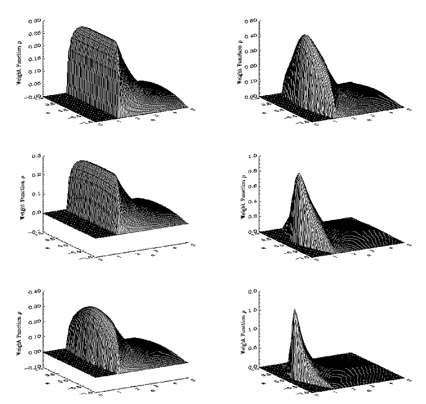
Figure 2: Development of the weight function as the bound state mass increases towards threshold. The left column contains the cases $\eta$=0,0.2 and 0.6, while the right hand column contains the cases $\eta$=0.8,0.95 and 0.99.

Figure 3: Comparison of the weight functions for a ladder kernel (top figure) and a dressed ladder kernel (bottom figure).

4 Conclusions and Outlook

We have formulated the BSE in Minkowski space for a completely general scattering kernel. This has been solved numerically for the ladder and dressed ladder kernels; both sets of results agree to high accuracy with results using more traditional Euclidean space methods.

We are currently implementing a kernel code which will enable us to numerically solve the scalar BSE for a completely general scalar kernel. As a first application of this code, we will solve for a “generalised ladder” kernel $\!{}^{{\bf?}}$. The Wick rotation is invalid in this case and so solution of the BSE in Minkowski space is essential in this instance.

To study problems of more general interest, it will be essential to extend the PTIR to theories containing fermions, and to find a way of incorporating confinement and derivative coupling into our approach. This will enable us to carry out studies of mesons in QCD, for example.

References

References

- [1]
- [2] E.E. Salpeter and H.A. Bethe, Phys. Rev. 84, 1232 (1951).
- [3] G.C. Wick, Phys. Rev. 96, 1124 (1954).
- [4] N. Nakanishi, Graph Theory and Feynman Integrals. Gordon and Breach, New York, 1971.
- [5] E. zur Linden and H. Mitter, Nuovo Cimento 61B, 389 (1969).
- [6] K. Kusaka and A.G. Williams, Phys. Rev. D 51, 7026 (1995).
- [7] K. Kusaka, K.M. Simpson and A.G. Williams, in preparation.