Abstract

We explore two possible interpretations for the CDF $ee\gamma\gamma+E_{T}\hskip-13.0pt/\quad$ event in the context of a recently proposed one-parameter no-scale supergravity model with a light gravitino. We delineate the region in parameter space consistent with the kinematics of the event interpreted either as selectron pair-production ($p\bar{p}\to\tilde{e}^{+}\tilde{e}^{-}\,X$, $\tilde{e}=\tilde{e}_{R},\tilde{e}_{L}$) or as chargino pair-production ($p\bar{p}\to\chi^{+}_{1}\chi^{-}_{1}\,X$). In the context of this model, the selectron interpretation requires $\tilde{e}=\tilde{e}_{R}$ and predicts comparable rates for $\ell^{\pm}\gamma\gamma+E_{T}\hskip-13.0pt/\quad$, whereas the chargino interpretation predicts comparable rates for $(\ell^{\pm}\ell^{{}^{\prime}+}\ell^{{}^{\prime}-},\ell^{+}\ell^{-},\ell^{+}\ell^{-}jj)\,\gamma\gamma+E_{T}\hskip-13.0pt/\quad$. We also consider the constraints from LEP 1.5 and the expectations for LEP 2. We point out that one of the acoplanar photon pairs observed by the OPAL collaboration at LEP 1.5 may be attributable to supersymmetry in the present model via $e^{+}e^{-}\to\chi^{0}_{1}\chi^{0}_{1}\to\gamma\gamma+E_{T}\hskip-13.0pt/\quad$. We also show how similar future events at LEP 2 may be used to deduce the neutralino mass.

1 Introduction

After the stunning confirmation of the Standard Model predictions at the Tevatron and LEP 1, the field of contenders for the much anticipated ‘new physics’ has, in the minds of most, been narrowed down to just one: supersymmetry. However, the many years elapsed since the invention of supersymmetry have produced abundant theoretical speculation as to the specific nature of supersymmetry, its origins, its breaking, and the spectrum of superparticles. Recent observations at the Tevatron, in the form of a puzzling $ee\gamma\gamma+E_{T}\hskip-13.0pt/\quad$ event [1], appear to indicate that experiment may have finally reached the sensitivity required to observe the first direct manifestations of supersymmetry [2, 3, 4]. If this event is indeed the result of an underlying supersymmetric production process, as might be deduced from the observation of additional related events at the Tevatron or LEP 2, it will herald a new era in elementary particle physics. The prima facie evidence for supersymmetry contains the standard missing-energy characteristic of supersymmetric production processes, but it also contains a surprising hard-photon component (as far as the Minimal Supersymmetry Standard Model is concerned), which eliminates all conceivable Standard Model backgrounds and may prove extremely discriminating among different models of low-energy supersymmetry.

The present supersymmetric explanations of the CDF event fall into two phenomenological classes: either the lightest neutralino ($\chi^{0}_{1}$) is the lightest supersymmetric particle, and the second-to-lightest neutralino decays radiatively to it at the one-loop level ($\chi^{0}_{2}\to\chi^{0}_{1}\gamma$); or the gravitino ($\widetilde{G}$) is the lightest supersymmetric particle, and the lightest neutralino decays radiatively to it at the tree level ($\chi^{0}_{1}\to\widetilde{G}\gamma$). The former ‘neutralino-LSP’ scenario requires a configuration of gaugino masses that precludes the usual gaugino mass unification relation of unified models, although it can occur in some restricted region of the MSSM parameter space. The latter ‘gravitino-LSP’ scenario requires only that the lightest neutralino has a photino component, as is typically the case in many supersymmetric models. The underlying process that leads to such final states has been suggested to be that of selectron pair-production ($q\bar{q}\to\widetilde{e}^{+}\widetilde{e}^{-}$, $\widetilde{e}=\widetilde{e}_{R},\widetilde{e}_{L}$), with subsequent decay $\widetilde{e}\to e\chi^{0}_{2}$ or $\widetilde{e}\to e\chi^{0}_{1}$ in the neutralino-LSP and gravitino-LSP scenarios respectively. In the gravitino-LSP scenario, the alternative possibility of chargino pair-production ($q\bar{q}\to\chi^{+}_{1}\chi^{-}_{1}$,$\chi^{\pm}_{1}\to e^{\pm}\nu_{e}\chi^{0}_{1}$) has also been briefly mentioned [5] (this possibility is not available in the neutralino-LSP scenario [6]).

Of these two classes of explanations, only the gravitino-LSP one has generated model-building efforts that try to embed such a scenario into a more fundamental theory at higher mass scales. These more predictive theories include low-energy gauge-mediated dynamical supersymmetry breaking [2, 7] and no-scale supergravity [4]. In this paper we study in detail the kinematics of the observed event in both the selectron and chargino interpretations in the context of our recently proposed one-parameter no-scale supergravity model [4]. We delineate the regions in parameter space that are consistent with the kinematical information, and then consider the rates for the various underlying processes that may occur within such regions of parameter space. Non-observation of related signals (e.g., $e\gamma\gamma+E_{T}\hskip-13.0pt/\quad$) that are predicted to occur at significantly higher rates than the presumably observed one (i.e., $ee\gamma\gamma+E_{T}\hskip-13.0pt/\quad$) imposes important constraints on the parameter space of the model. It should be noted that the possibility of observing supersymmetry at the Tevatron via weakly-interacting production processes had been shown early on to be particularly favorable in the context of no-scale supergravity [8]. We also consider the constraints from LEP 1.5 and the prospects for supersymmetric particle detection at LEP161 and LEP190. We show that one of the acoplanar photon pairs observed by the OPAL collaboration at LEP 1.5 may be attributable to supersymmetry in the present model via $e^{+}e^{-}\to\chi^{0}_{1}\chi^{0}_{1}\to\gamma\gamma+E_{T}\hskip-13.0pt/\quad$. We should remark that because of the rather restrictive nature of our one-parameter model, our experimental predictions are unambiguous and highly correlated.

This paper is organized as follows. In Section 2 we review the basic model predictions and expand on the motivation for our model and its significance in the context of no-scale supergravity, flipped SU(5), and extended supergravities. In Sec. 3 we consider the CDF event from the perspective of the selectron and chargino interpretation, delineate the allowed regions in parameter space, and contrast the rates for related processes that might have been observed. In Sec. 4 we determine the constraints from LEP 1.5, study in some detail the OPAL acoplanar photon events, and explore the prospects for particle detection at LEP 2. In Sec. 5 we summarize our conclusions.

2 The model

2.1 Motivation

Supergravity models are described in terms of two functions, the Kähler function $G=K+\ln|W|^{2}$, where $K$ is the Kähler potential and $W$ the superpotential; and the gauge kinetic function $f$. Specification of these functions determines the supergravity interactions and the soft supersymmetry-breaking parameters that arise after spontaneous breaking of supergravity, which is parametrized by the gravitino mass $m_{3/2}=e^{K/2}\,|W|$. In standard supergravity scenarios the choices for $G$ and $f$ may follow from symmetry considerations or may be calculated in certain weakly-coupled heterotic string vacua (such as orbifolds or free-fermionic constructions). In these cases one generically obtains soft-supersymmetry-breaking parameters (i.e., scalar and gaugino masses and scalar interactions) that are comparable to the gravitino mass: $m_{0},m_{1/2},A_{0}\sim m_{3/2}$, although the specific proportionality coefficients in these relations may vary in magnitude and may even be non-universal. In the context of unified models, such standard scenarios do not appear to be consistent with a supersymmetric explanation of the CDF $ee\gamma\gamma+E_{T}\hskip-13.0pt/\quad$ event because, either the implied gaugino mass unification is violated (neutralino-LSP scenario), or the required light gravitino mass (i.e., $m_{3/2}\ll 1\,{\rm GeV}$) would render all supersymmetric particles comparably light (gravitino-LSP scenario).

In the gravitino-LSP scenario, the main issue is that of decoupling the breaking of local supersymmetry (parametrized by $m_{3/2}$) from the breaking of global supersymmetry (parametrized by $m_{0},m_{1/2}$). This decoupling is achieved naturally in the context of no-scale supergravity [9, 10], where a judicious choice of the Kähler potential ($K$) yields $m_{0}=0m_{3/2}$ (and also $A_{0}=B_{0}=0$), which allows a very wide range of $m_{3/2}$ values. (No-scale supergravity is also obtained in weakly-coupled string models, as was shown early on by Witten [11] and has more recently been explored in great detail in Ref. [12].) Without this (scalar-sector) decoupling, sizeable values of $m_{0}$ (i.e., $m_{0}\sim M_{Z}$) cannot be obtained in the light gravitino scenario. As we discuss below, the selectron interpretation of the CDF event requires $m_{0}\ll M_{Z}$ [4], but there is no such requirement for the chargino interpretation. In this connection we should add that in unified models the possible values of $m_{0}/m_{1/2}$ are constrained by the proton decay rate via dimension-five operators. In the minimal SU(5) supergravity model one can show that $m_{0}/m_{1/2}>3$ is required [13], thus rendering this decoupling impossible. In contrast, in flipped SU(5) such operators are naturally suppressed, and $m_{0}=0$ is perfectly allowed [14].

2.2 A light gravitino

The remaining and crucial question is the decoupling in the gaugino sector, that depends on the choice of $f$, at least in traditional supergravity models. The gaugino masses are given by

$$m_{1/2}=m_{3/2}\left({\partial_{z}f\over 2{\rm Re}f}\right)\left({\partial_{z}G\over\partial_{zz^{*}}G}\right)\ ,$$ (1)

where $z$ represents the hidden sector (moduli) fields in the model, and the gaugino mass universality at the Planck scale is insured by a gauge-group independent choice for $f$. As remarked above, the usual expressions for $f$ (e.g., in weakly-coupled string models) give $m_{1/2}\sim m_{3/2}$. This result is however avoided by considering the non-minimal choice $f\sim e^{-Az^{q}}$, where $A,q$ are constants [15]. Assuming the standard no-scale expression $G=-3\ln(z+z^{*})$, one can then readily show that [15]

$$m_{1/2}\sim\left({m_{3/2}\over M}\right)^{1-{2\over 3}q}M\ ,$$ (2)

where $M\approx 10^{18}\,{\rm GeV}$ is the rescaled Planck mass. The phenomenological requirement of $m_{1/2}\sim 10^{2}\,{\rm GeV}$ then implies ${3\over 4}\raisebox{-4.0pt}{$\,\stackrel{{\scriptstyle\textstyle{>}}}{{\sim}}\,$}q\raisebox{-4.0pt}{$\,\stackrel{{\scriptstyle\textstyle{>}}}{{\sim}}\,$}{1\over 2}$ for $10^{-5}\,{\rm eV}\raisebox{-4.0pt}{$\,\stackrel{{\scriptstyle\textstyle{<}}}{{\sim}}\,$}m_{3/2}\raisebox{-4.0pt}{$\,\stackrel{{\scriptstyle\textstyle{<}}}{{\sim}}\,$}10^{3}\,{\rm eV}$. Note that $q={3\over 4}$ gives the relation $m_{3/2}\sim m^{2}_{1/2}/M\sim 10^{-5}\,{\rm eV}$, which was obtained very early on in Ref. [16] from the perspective of hierarchical supersymmetry breaking in extended N=8 supergravity. The recent theoretical impetus for supersymmetric M-theory in 11 dimensions may also lend support to this result, as N=1 in D=11 corresponds to N=8 in D=4.

More specifically, the needed decoupling between the local and global breaking of supersymmetry, that we have advocated above in order to insure a light gravitino, appears to be realized in strongly coupled heterotic strings [17], which are best understood in terms of 11-dimensional supergravity. Moreover, the no-scale supergravity structure appears to also emerge in strongly-coupled strings [18, 17] and to take on a crucial role in suppressing the cosmological constant at the classical [9, 10] and quantum levels [17, 19], as well as avoiding flavor-changing neutral currents [18, 19]. These general remarks should sufficiently motivate our present phenomenological study.

2.3 The spectrum

Our model effectively fits within the usual no-scale supergravity models with universal soft-supersymmetry-breaking parameters given by

$$m_{0}=A_{0}=B_{0}=0\ .$$ (3)

When the constraints from radiative electroweak symmetry breaking are imposed, the values of $|\mu|$ and $B(M_{Z})$ are determined (for the fixed value of $m_{t}=175\,{\rm GeV}$). Evolving the latter up to the Planck scale, and demanding that it reproduce the boundary condition $B_{0}=0$, determines the value of $\tan\beta$ in terms of the single parameter of the model ($m_{1/2}$). One can show that the sign of $\mu$ is also determined by this procedure [20].

The precise low-energy spectrum of the model further depends on the details of the evolution between the Planck scale and the electroweak scale. One may envision a traditional scenario where unification occurs at the usual GUT scale ($M_{\rm LEP}\sim 10^{16}\,{\rm GeV}$), while supersymmetry breaking is communicated to the observable sector at the Planck scale. Alternatively one may supplement the MSSM spectrum with intermediate-scale particles that delay unification up to the Planck scale [21]. A third and perhaps more realistic scenario combines both approaches and has been recently realized in flipped SU(5) [22], achieving a partial unification at $M_{\rm LEP}$ [SU(2)$\times$SU(3)$\to$SU(5)] and string unification at $M_{Pl}$. However, this scenario depends on various parameters which make the analysis more complicated that needs to be at this stage. Here we opt for the second scenario, where unification occurs in a single step at the Planck scale. We expect that our numerical results will remain qualitatively unchanged in any of these three possible unification scenarios.

The spectrum as a function of the lightest neutralino mass is given in Fig. 1 for the lighter particles (sleptons, lightest higgs boson, lighter neutralinos and charginos) and in Fig. 2 for the heavier particles (gluino, squarks, heavy higgs bosons, heavier neutralinos and charginos). The calculated value of $\tan\beta$ as a function of $m_{\chi^{0}_{1}}$ is displayed in Fig. 1. We also find that $|\mu|\approx m_{\chi^{0}_{3}}$, which can then be obtained from Fig. 2. These figures show that the lightest neutralino (which is mostly bino) is always the next-to-lightest supersymmetric particle (NSLP), followed by the right-handed sleptons ($\tilde{e}_{R},\tilde{\mu}_{R},\tilde{\tau}_{1}$), the lighter neutralino/chargino ($\chi^{0}_{2},\chi^{\pm}_{1}$), the sneutrino ($\tilde{\nu}$), and the left-handed sleptons ($\tilde{e}_{L},\tilde{\mu}_{L},\tilde{\tau}_{2}$). (The order of the second and third elements on this list is reversed for very light neutralino masses.) Note the splitting between the selectron/smuon masses and the stau mass due to the non-negligible value of the $\lambda_{\tau}$ Yukawa coupling. The lightest higgs boson crosses all sparticle lines and is in the range $m_{h}=(100-120)\,{\rm GeV}$. Also notable is that the average squark mass ($\tilde{q}$) is slightly below the gluino mass ($\tilde{g}$) and the lightest top-squark ($\tilde{t}_{1}$) is somewhat lighter than both of these.

As emphasized early on [15], the dominant decay of the lightest neutralino is via $\chi^{0}_{1}\to\gamma\widetilde{G}$, which has partial a width of [15, 5]

$$\Gamma(\chi^{0}_{1}\to\gamma\widetilde{G})={\kappa_{1\gamma}\over 48\pi}\,{m^{5}_{\chi^{0}_{1}}\over(M_{Pl}\,m_{\widetilde{G}})^{2}}=1.12\times 10^{-11}\,{\rm GeV}\kappa_{1\gamma}\left({m_{\chi^{0}_{1}}\over 100\,{\rm GeV}}\right)^{5}\left({m_{\widetilde{G}}\over 1\,{\rm eV}}\right)^{-2}\ ,$$ (4)

where $\kappa_{1\gamma}=|N_{11}\cos\theta_{W}+N_{12}\sin\theta_{W}|^{2}$ is the square of the photino admixture of the lightest neutralino. In our model $\kappa_{1\gamma}>0.5,0.6,0.7$ for $m_{\chi^{0}_{1}}>40,55,85\,{\rm GeV}$, with a maximum value of 0.74, attained asymptotically when the lightest neutralino approaches a pure bino. The decay $\chi^{0}_{1}\to Z\widetilde{G}$, accessible for $m_{\chi^{0}_{1}}>M_{Z}$, is greatly suppressed by the $\beta^{8}$ threshold behavior [5]; we find $\Gamma(\chi^{0}_{1}\to Z\widetilde{G})/\Gamma(\chi^{0}_{1}\to\gamma\widetilde{G})<0.03$. The decay $\chi^{0}_{1}\to h\widetilde{G}$ may also be accessible (for $m_{\chi^{0}_{1}}>120\,{\rm GeV}$) but it is completely negligible because of the above kinematical suppression and because of the gaugino nature of the neutralino. In sum, we expect $B(\chi^{0}_{1}\to\gamma\widetilde{G})\approx 100\%$ throughout the whole parameter space. One can also consider the probability for $\chi^{0}_{1}$ (with energy $E$) to travel a distance $x$ before decaying $P(x)=1-e^{-x/L}$, where the decay length is given by [5]

$$L=1.76\times 10^{-3}\,(\kappa_{1\gamma})^{-1}\left(E^{2}/m^{2}_{\chi^{0}_{1}}-1\right)^{1/2}\left({m_{\chi^{0}_{1}}\over 100\,{\rm GeV}}\right)^{-5}\left({m_{\widetilde{G}}\over 1\,{\rm eV}}\right)^{2}\,{\rm cm}\ .$$ (5)

The requirement $m_{3/2}\raisebox{-4.0pt}{$\,\stackrel{{\scriptstyle\textstyle{<}}}{{\sim}}\,$}250\,{\rm eV}$ ensures a visible neutralino decay within the CDF (or any other such) detector [3].

3 The CDF event

We now turn to the implications of the observed CDF $ee\gamma\gamma+E_{T}\hskip-13.0pt/\quad$ event, assuming that it is the result of an underlying supersymmetric production process in the context of our present model. The particulars of the event are listed in Table 1. We consider two interpretations (selectron and chargino pair production), in each case delineating the region in parameter space consistent with the observed kinematics of the event. We then determine the rate for such processes and for related processes with similar signatures that might have also been detected.

3.1 Selectron interpretation

In this interpretation one assumes that the underlying process is $q\bar{q}\to\widetilde{e}^{+}_{R}\widetilde{e}^{-}_{R}$ or $q\bar{q}\to\widetilde{e}^{+}_{L}\widetilde{e}^{-}_{L}$, as shown in Figs. 3(a) and 3(b) respectively. The selectrons subsequently decay via $\widetilde{e}^{\pm}_{R,L}\to e^{\pm}\chi^{0}_{1}$ [Fig. 3(e)] with $100\%$ branching ratio, and the neutralinos further decay via $\chi^{0}_{1}\to\gamma\widetilde{G}$ [Fig. 3(g)], also with $100\%$ branching ratio. The final state thus contains $e^{+}e^{-}\gamma\gamma\widetilde{G}\widetilde{G}$, with the (essentially) massless gravitinos carrying away the missing energy.

The kinematical data shown in Table 1 constrain the possible masses of the selectron ($m_{\tilde{e}_{R,L}}$) and neutralino ($m_{\chi^{0}_{1}}$). To obtain these constraints we perform a Monte Carlo simulation of the process in which we vary at random the three-momenta of the unobserved gravitinos, subject to the constraints of transverse momentum conservation (up the $E_{T}\hskip-13.0pt/\quad$ ‘vector’ given in Table 1) and equality of neutralino and selectron masses in each decay. We have considered the two possible pairings of the photons and electrons (i.e., which $e$ and $\gamma$ go with $\widetilde{e}^{+}$ and which go with $\widetilde{e}^{-}$) but find that only one pairing satisfies all consistency constraints. We thus obtain a $2\times 3-2-1-1=2$–dimensional solution space that parametrizes the two unknown masses. The resulting allowed region in $(m_{\tilde{e}_{R,L}},m_{\chi^{0}_{1}}$) space is found to be partially bounded, and with a sufficiently dense sample of Monte Carlo points one can determine its boundary, as shown in Fig. 4. The region in principle continues onto larger sparticles masses, but we have cut it off (vertical line) at $m_{\tilde{e}}=150\,{\rm GeV}$ because the predicted rates at the Tevatron become uninterestingly small beyond that point. Within the closed region we see that underlying $\widetilde{e}_{L}$ pair-production is disfavored. On the other hand, underlying $\widetilde{e}_{R}$ pair-production is perfectly consistent with the kinematics of the event, with the further constraints

$$m_{\tilde{e}_{R}}\approx(85-135)\,{\rm GeV}\ ,\quad m_{\chi^{0}_{1}}\approx(50-100)\,{\rm GeV}\ .$$ (6)

Model mass relations (see Fig. 1) then imply $m_{\chi^{\pm}_{1}}\approx(90-190)\,{\rm GeV}$.

Table 1: The kinematical information of the observed CDF $ee\gamma\gamma+E_{T}\hskip-13.0pt/\quad$ event. All momenta and energies in GeV. Also important are $E_{T}\hskip-13.0pt/\quad=52.81\,{\rm GeV}$ at $\phi=2.91\,{\rm rad}$.

Variable	$e_{1}\quad$	$e_{2}\quad$	$\gamma_{1}\quad$	$\gamma_{2}\quad$
$p_{x}$	$58.75$	$-33.41$	$-12.98$	$31.53$
$p_{y}$	$18.44$	$11.13$	$-29.68$	$-17.48$
$p_{z}$	$-167.24$	$21.00$	$-22.69$	$-34.77$
$E$	$178.21$	$41.00$	$39.55$	$50.09$
$E_{T}$	$61.58$	$35.21$	$32.39$	$36.05$

 

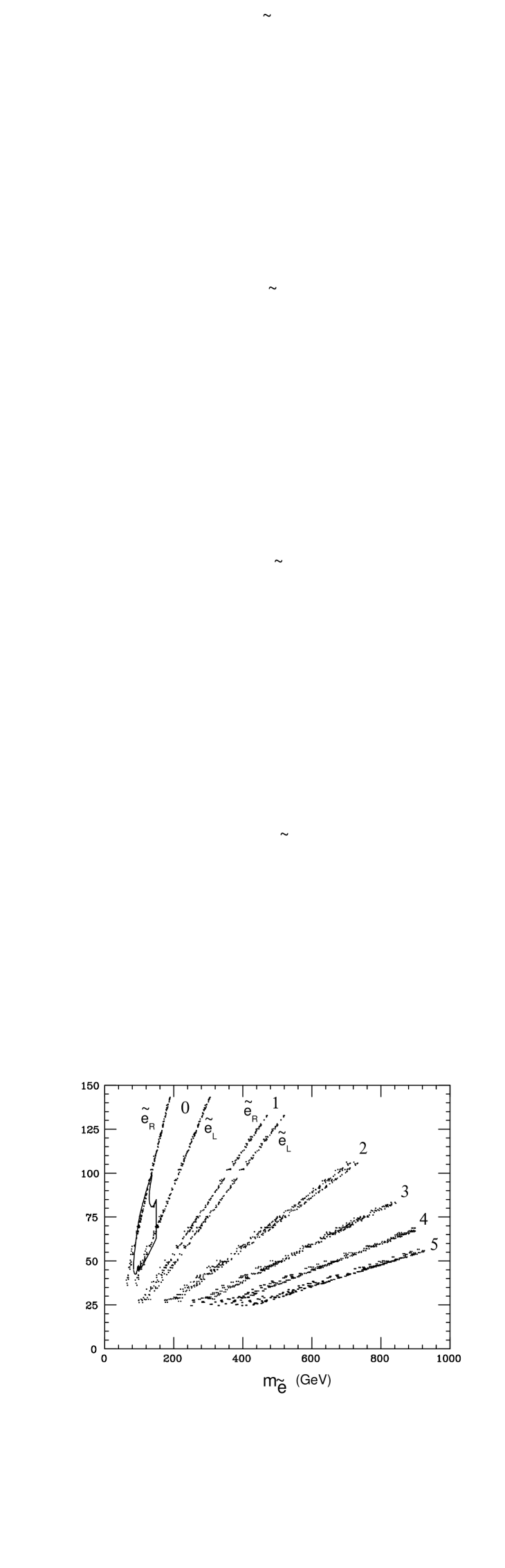
Figure 5: Calculated distribution of selectron ($\tilde{e}$) and lightest neutralino ($\chi^{0}_{1}$) masses in generic supergravity models for fixed values of the ratio $\xi_{0}=m_{0}/m_{1/2}=0,1,2,3,4,5$; and varying values of $\{m_{1/2},\tan\beta,A_{0}\}$. The area within the closed region is consistent with the kinematics and dynamics of the CDF $ee\gamma\gamma$ event. The branches for $\tilde{e}_{R}$ and $\tilde{e}_{L}$ are only distinguishable for $\xi_{0}=0,1$. Our model predicts $\xi_{0}=0$.

Before proceeding with the analysis, it is instructive to determine what other sets of standard supergravity parameters $\{m_{0},m_{1/2},A_{0},\tan\beta\}$ may also be consistent with the kinematics of the CDF event in the selectron interpretation. We have generated 10,000 different random four-parameter sets of this kind, and in each case determined the low-energy spectrum, in particular the $\chi^{0}_{1}$ and $\tilde{e}_{R,L}$ masses. As we just showed, the kinematics of the event singles out an allowed region in the $(m_{\tilde{e}},m_{\chi^{0}_{1}})$ plane (see Fig. 4). In Fig. 5 we show the distribution of models in this space, with the preferred region bounded by the solid line. For clarity, in the figure we restrict the choices of $\xi_{0}=m_{0}/m_{1/2}$ to the integer values shown (i.e., $0\to 5$), with the other three parameters allowed to vary at random. (The branches for $\tilde{e}_{R}$ and $\tilde{e}_{L}$ are only distinguishable for $\xi_{0}=0,1$.) This figure illustrates the fraction of the generic supergravity parameter space that is consistent with the kinematics of the CDF event. Moreover, our model prediction of $\xi_{0}=0$ clearly falls within the allowed region for both $\tilde{e}_{R}$ and $\tilde{e}_{L}$, whereas $\xi_{0}\geq 1$ is not allowed. Note that the actual model prediction for $\widetilde{e}_{L}$ (as shown in Fig. 4) has much less of an overlap with the allowed region than the generic $m_{0}=0$ result in Fig. 5. This is due to the additional model constraints that correlate all four parameters, leaving only one to vary freely.

We now turn to the dynamics of the selectron interpretation. We consider the production of the four slepton channels:

$$q\bar{q}\to\gamma,Z\to\widetilde{\ell}^{+}_{R}\widetilde{\ell}^{-}_{R},\widetilde{\ell}^{+}_{L}\widetilde{\ell}^{-}_{L}\to(\ell^{+}\chi^{0}_{1})(\ell^{-}\chi^{0}_{1})\to\ell^{+}\ell^{-}\gamma\gamma+E_{T}\hskip-13.0pt/\quad\$$ (7)

$$q\bar{q}^{\prime}\to W^{\pm}\to\widetilde{\ell}^{\pm}_{L}\widetilde{\nu}_{\ell}\to(\ell^{\pm}\chi^{0}_{1})(\nu_{\ell}\chi^{0}_{1})\to\ell^{\pm}\gamma\gamma+E_{T}\hskip-13.0pt/\quad,$$ (8)

$$q\bar{q}\to Z\to\widetilde{\nu}_{\ell}\widetilde{\nu}_{\ell}\to(\nu_{\ell}\chi^{0}_{1})(\nu_{\ell}\chi^{0}_{1})\to\gamma\gamma+E_{T}\hskip-13.0pt/\quad,$$ (9)

where $\ell=e,\mu,\tau$ [see Figs. 3(a,b,c,d)], and we have indicated the experimental signature in each case ($E_{T}\hskip-13.0pt/\quad$ includes the two gravitinos from $\chi^{0}_{1}\to\gamma\widetilde{G}$ decay and may also include neutrinos). We have calculated the corresponding hadronic cross sections using the parton-level differential cross sections given in Ref. [23], and integrated them over phase space and parton distribution functions. The resulting cross sections for $\ell=e$ are shown in Fig. 6 as a function of the selectron mass. The same result is obtained for $\ell=\mu$ or $\ell=\tau$, i.e., one would multiply the curves in Fig. 6 by a factor of 3 to obtain the cross section summed over the three flavors. We should note that because the slepton ($\widetilde{\ell}_{R},\widetilde{\ell}_{L},\widetilde{\nu}_{\ell}$) masses are correlated in the specific way shown in Fig. 1, the resulting relations between the different slepton rates differ from those naively obtained when the slepton masses of the same flavor are taken to be all equal. For instance, when $m_{\tilde{e}_{L}}=m_{\tilde{e}_{R}}$ one finds $\sigma(\tilde{e}_{L}\tilde{e}_{L})\approx 2.3\,\sigma(\tilde{e}_{R}\tilde{e}_{R})$, whereas in our case $\sigma(\tilde{e}_{L}\tilde{e}_{L})<\sigma(\tilde{e}_{R}\tilde{e}_{R})$ always.

As noted in Eqs. (7,8,9), the experimental signatures for these four channels differ in the number of charged leptons: 2,1,0 respectively. In Fig. 7 we show the correlation between the number of single-lepton versus the number of di-lepton events that are expected in ${\cal L}=100\,{\rm pb}^{-1}$ of data. At the one dilepton-event level, the expected number of single-lepton events (two) is still consistent with observation (zero). However, possible observation of more $ee\gamma\gamma+E_{T}\hskip-13.0pt/\quad$ events would need to be accompanied by many more $e\gamma\gamma+E_{T}\hskip-13.0pt/\quad$ events. On the top axis of the plot we show the corresponding selectron mass, which shows that one event is consistent with $m_{\tilde{e}_{R}}$ as high as 100 GeV. (However, one should realize $N(ee\gamma\gamma+E_{T}\hskip-13.0pt/\quad)$ in Fig. 7 includes both $\tilde{e}_{R}$ and $\tilde{e}_{L}$ sources, although the former dominates over the latter and the latter is kinematically inconsistent with the observed event.) It has been advocated that $1\over 2$ event should mark the minimum event rate consistent with the observations [7, 5], in this case we find the upper bound $m_{\tilde{e}_{R}}<115\,{\rm GeV}$. This limit may be weakened to $m_{\tilde{e}_{R}}<150\,{\rm GeV}$ by summing over slepton flavors, although it is not clear what the meaning of this procedure is.

In Fig. 7 we also show the number of diphoton (no-lepton) events, which is seen to be negligible at the one dilepton-event level, but should quickly overtake the number of dilepton events should more of these be observed. As a final comment on the viability of the selectron interpretation, we should remark that one must require a rather substantive chargino mass ($m_{\chi^{\pm}_{1}}>125\,{\rm GeV}$ [5]) so that the additional sources of $ee\gamma\gamma+E_{T}\hskip-13.0pt/\quad$ events from chargino/neutralino production (see Sec. 3.2) remain below the few-event level. Through the mass relations in this model (see Fig. 1), this requirement entails $m_{\tilde{e}_{R}}>100\,{\rm GeV}$ and $m_{\chi^{0}_{1}}>68\,{\rm GeV}$, which are still consistent with the selectron interpretation.

3.2 Chargino interpretation

One may envision an alternative interpretation of the $ee\gamma\gamma+E_{T}\hskip-13.0pt/\quad$ event wherein the underlying process is assumed to be $q\bar{q}\to\chi^{+}_{1}\chi^{-}_{1}$ as shown in Figs. 8(a,b). The charginos subsequently decay via $\chi^{\pm}_{1}\to e^{\pm}\nu_{e}\chi^{0}_{1}$ [see Fig. 9(c,d,e)] with some calculable branching ratio, and the neutralinos further decay via $\chi^{0}_{1}\to\gamma\widetilde{G}$ [Fig. 3(g)] with $100\%$ branching ratio. The final state thus contains $e^{+}e^{-}\gamma\gamma\nu_{e}\bar{\nu}_{e}\widetilde{G}\widetilde{G}$, with the (essentially) massless gravitinos and the neutrinos carrying away the missing energy.

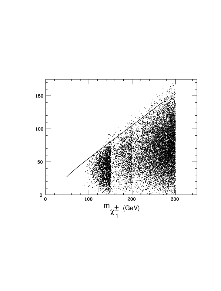
Figure 11: Region consistent with the kinematics of the CDF $ee\gamma\gamma+E_{T}\hskip-13.0pt/\quad$ event when interpreted as chargino ($\chi^{\pm}_{1}$) pair production: each chargino decays to $e\nu_{e}\chi^{0}_{1}$ and each neutralino decays to photon and gravitino ($\gamma\widetilde{G}$). Kinematics requires $m_{\chi^{\pm}_{1}}>95\,{\rm GeV}$. The solid line represents the model prediction, which is consistent with the kinematics of the event for $m_{\chi^{\pm}_{1}}>100\,{\rm GeV}$ and $m_{\chi^{0}_{1}}>55\,{\rm GeV}$.

In analogy with the selectron interpretation, the kinematical data shown in Table 1 constrain the possible masses of the chargino ($m_{\chi^{\pm}_{1}}$) and neutralino ($m_{\chi^{0}_{1}}$). (These constraints hold irrespective of the dynamics of the process, i.e., the underlying cross section and branching ratios.) However, in the chargino interpretation we have four missing momenta, and the constraints from tranverse momentum conservation and equality of neutralino and chargino masses in each decay allow a vast $4\times 3-2-1-1=8$–dimensional solution space. We find that both possible pairings of the photons and electrons (i.e., which $e$ and $\gamma$ go with $\chi^{+}_{1}$ and which go with $\chi^{-}_{1}$) satisfy all consistency constraints. The resulting allowed region in $(m_{\chi^{\pm}_{1}},m_{\chi^{0}_{1}}$) space is difficult to delineate, but as far as we can tell it is partially bounded requiring $m_{\chi^{\pm}_{1}}>95\,{\rm GeV}$, as shown in Fig. 11. The figure also shows that the model prediction (solid line) does intercept the kinematically allowed region, starting at $m_{\chi^{\pm}_{1}}\approx 100\,{\rm GeV}$ and $m_{\chi^{0}_{1}}\approx 55\,{\rm GeV}$. The dynamics of the event further restricts the allowed interval, as we discuss below.

We would like to digress briefly to comment on other sets of standard supergravity parameters $\{m_{0},m_{1/2},A_{0},\tan\beta\}$ that may also be consistent with the kinematics of the event in the chargino interpretation. Following the same procedure as in the selectron interpretation, we find the well-known result in supergravity models that $m_{\chi^{\pm}_{1}}\approx 2m_{\chi^{0}_{1}}$. Therefore, basically any standard supergravity model that allows $m_{\chi^{\pm}_{1}}>100\,{\rm GeV}$ will be consistent with the kinematical constraints of the event in the chargino interpretation. Of course the dynamics of the event (light gravitino, suitable cross section and branching ratios) will be a lot more discriminating. For instance, any value of $m_{0}$ would appear acceptable from the kinematics alone. However, $m_{0}$ affects the branching ratios and may not enhance the desired leptonic decays of the chargino. Also, as discussed in Sec. 2.1, a non-negligible value of $m_{0}$ is not attainable in supergravity models with a light gravitino.

We now turn to the dynamics of the chargino interpretation. We consider the production of the following chargino/neutralino channels:

$$q\bar{q}\to\chi^{+}_{1}\chi^{-}_{1}\to\left\{\begin{array}[]{l}(\ell^{+}\nu_{\ell}\chi^{0}_{1})(\ell^{-}\bar{\nu}_{\ell}\chi^{0}_{1})\to\ell^{+}\ell^{-}\gamma\gamma+E_{T}\hskip-13.0pt/\\ (\ell^{\pm}\nu_{\ell}\chi^{0}_{1})(q\bar{q}^{\prime}\chi^{0}_{1})\to\ell^{\pm}\,jj\,\gamma\gamma+E_{T}\hskip-13.0pt/\\ (q\bar{q}^{\prime}\chi^{0}_{1})(q^{\prime}\bar{q}\chi^{0}_{1})\to jjjj\,\gamma\gamma+E_{T}\hskip-13.0pt/\end{array}\right.$$ (13)

$$q\bar{q}^{\prime}\to\chi^{\pm}_{1}\chi^{0}_{2}\to\left\{\begin{array}[]{l}(\ell^{\pm}\nu_{\ell}\chi^{0}_{1})(\ell^{{}^{\prime}+}\ell^{{}^{\prime}-}\chi^{0}_{1})\to\ell^{\pm}\ell^{{}^{\prime}+}\ell^{{}^{\prime}-}\,\gamma\gamma+E_{T}\hskip-13.0pt/\\ (\ell^{\pm}\nu_{\ell}\chi^{0}_{1})(\nu_{\ell}\bar{\nu}_{\ell}\chi^{0}_{1})\to\ell^{\pm}\,\gamma\gamma+E_{T}\hskip-13.0pt/\\ (q\bar{q}^{\prime}\chi^{0}_{1})(\ell^{+}\ell^{-}\chi^{0}_{1})\to\ell^{+}\ell^{-}\,jj\,\gamma\gamma+E_{T}\hskip-13.0pt/\\ (\ell^{\pm}\nu_{\ell}\chi^{0}_{1})(q\bar{q}\chi^{0}_{1})\to\ell^{\pm}\,jj\,\gamma\gamma+E_{T}\hskip-13.0pt/\\ (q\bar{q}^{\prime}\chi^{0}_{1})(\nu_{\ell}\bar{\nu}_{\ell}\chi^{0}_{1})\to jj\,\gamma\gamma+E_{T}\hskip-13.0pt/\\ (q\bar{q}^{\prime}\chi^{0}_{1})(q\bar{q}\chi^{0}_{1})\to jjjj\,\gamma\gamma+E_{T}\hskip-13.0pt/\\ \end{array}\right.$$ (20)

$$q\bar{q}^{\prime}\to\chi^{\pm}_{1}\chi^{0}_{1}\to\left\{\begin{array}[]{l}\chi^{0}_{1}(\ell^{\pm}\nu_{\ell}\chi^{0}_{1})\to\ell^{\pm}\,\gamma\gamma+E_{T}\hskip-13.0pt/\\ \chi^{0}_{1}(q\bar{q}^{\prime}\chi^{0}_{1})\to jj\,\gamma\gamma+E_{T}\hskip-13.0pt/\\ \end{array}\right.$$ (23)

where $\ell,\ell^{\prime}=e,\mu,\tau$, and we have indicated the experimental signature in each case. We have not shown the $\chi^{0}_{2}\to h\chi^{0}_{1}$ decay channel [see Fig. 10(g)] as in our model it becomes kinematically accessible only for $m_{\chi^{0}_{2}}>m_{h}+m_{\chi^{0}_{1}}$ or $m_{\chi^{0}_{2}}>2m_{h}\approx 250\,{\rm GeV}$. Also, the additional production channels $q\bar{q}\to\chi^{0}_{i}\chi^{0}_{j}$ ($i,j=1,2$) shown in Fig. 8(e,f), proceed at much smaller rates: the $Z\chi^{0}_{i}\chi^{0}_{j}$ coupling is suppressed for our case of mostly gaugino-like neutralinos, and the $t$-channel diagrams are suppressed by heavy squark masses.

We have calculated the hadronic cross sections for the processes in Eqs. (13,20,23), and these are shown in Fig. 12 as a function of the chargino mass. We note that for not too small values of the chargino mass, the $\chi^{\pm}_{1}\chi^{0}_{2}$ and $\chi^{+}_{1}\chi^{-}_{1}$ channels dominate. However, $\chi^{\pm}_{1}\chi^{0}_{1}$ is not negligible and may give the dominant contribution to some signatures, as we discuss below.

The chargino and neutralino branching ratios are complicated functions of all model parameters, as the Feynman diagrams in Figs. 9 and 10 indicate. The numerical results as a function of the chargino mass are shown in Fig. 13, and may be understood as follows. In the case of the chargino decays, for low values of the chargino mass the $\ell^{\pm}\nu_{\ell}$ channel dominates, as the sneutrino-mediated decay [Fig. 9(d)] is enhanced by $m_{\tilde{\nu}}\approx m_{\chi^{\pm}_{1}}$ [see Fig. 1]. As the chargino mass increases the $W$-mediated decays become more important as the sneutrino becomes heavier than the chargino. Eventually the $W$-mediated decays fully dominate, and the expected branching ratios into leptons ($3/9$) and into quarks ($6/9$) are attained. (Note that in Fig. 13 we have summed over only two lepton families.)

In the case of neutralino decays, the pattern may also be understood in terms of the spectrum shown in Fig. 1. For low neutralino masses, the sneutrino-mediated decay [Fig. 10(f)] is on-shell and $\chi^{0}_{2}\to\nu_{\ell}\bar{\nu}_{\ell}\chi^{0}_{1}$ dominates. Soon thereafter the sneutrino goes off-shell, but the right-handed sleptons go on-shell and $\chi^{0}_{2}\to\ell^{+}\ell^{-}\chi^{0}_{1}$ dominates. This dominance continues until the decay $\chi^{0}_{2}\to Z\chi^{0}_{1}$ becomes accessible for $m_{\chi^{0}_{2}}\approx 2M_{Z}$ (as Fig. 13 shows). The influence of the $Z$-mediated channels continues until $m_{\chi^{0}_{2}}\approx 2m_{h}$, where the $\chi^{0}_{2}\to h\chi^{0}_{1}$ channel becomes accessible and completely dominant (such high values of $m_{\chi^{0}_{2}}$ are not shown in Fig. 13).

The actual signals are obtained by multiplying the cross sections times the branching ratios as indicated in Eqs. (13,20,23); these are shown in Fig. 14. This busy plot shows that the expected number of events without jets (solid lines) dominates over the number of events with 2 jets (dashed lines) or 4 jets (dotted line). The precise number of expected events depends on the experimental detection efficiencies for each of these signatures, and thus requires a detailed simulation including detector effects. One may get an idea of the number of expected events in ${\cal L}=100\,{\rm pb}^{-1}$ by simply assuming an across-the-board $10\%$ efficiency. In this approximation the numbers of expected events would be the numbers in Fig. 14 multiplied by $1/100$. These numbers of expected events should not exceed a few, as so far only one event of this kind has been observed at CDF. Consulting Fig. 14, it would appear reasonable to require $m_{\chi^{\pm}_{1}}>100\,{\rm GeV}$ (which implies $m_{\tilde{e}_{R}}>85\,{\rm GeV}$ and $m_{\chi^{0}_{1}}>55\,{\rm GeV}$). As discussed above (see Fig. 11), this lower bound is also required by the kinematics of the event. A reasonable upper bound in order to produce enough events would appear to be $m_{\chi^{\pm}_{1}}\approx 150\,{\rm GeV}$. Figure14 then shows that in this regime the dominant signals are $\ell^{\pm}\ell^{{}^{\prime}+}\ell^{{}^{\prime}-}+\gamma\gamma+E_{T}\hskip-13.0pt/\quad$ (including $e^{\pm}e^{+}e^{-},e^{+}e^{-}\mu^{\pm},e^{\pm}\mu^{+}\mu^{-},\mu^{\pm}\mu^{+}\mu^{-}$), $\ell^{+}\ell^{-}+\gamma\gamma+E_{T}\hskip-13.0pt/\quad$ (including $e^{+}e^{-},\mu^{+}\mu^{-}$), and $\ell^{+}\ell^{-}jj+\gamma\gamma+E_{T}\hskip-13.0pt/\quad$ (including $e^{+}e^{-}jj,\mu^{+}\mu^{-}jj$). Note that the single-flavor $3\ell$ and $2\ell$ signals (e.g., $e^{\pm}e^{+}e^{-}$ and $e^{+}e^{-}$) occur at nearly the same rate, as does the $\ell^{+}\ell^{-}jj$ signal given the uncertainty on the acceptances for these channels. (Decays involving $\ell=\tau$ are of course also expected to occur.)

Let us also remark on the importance of the $\chi^{\pm}_{1}\chi^{0}_{1}$ channel in Eq. (23), which contributes to the $1\ell$ and $2j$ signals in Fig. 14. Both these signals receive an additional contribution from $\chi^{\pm}_{1}\chi^{0}_{2}$, but only when the neutralino decays invisibly ($\chi^{0}_{2}\to\nu\bar{\nu}\chi^{0}_{1}$), which happens only for very light chargino masses [see Fig. 13]. For moderate chargino masses these signals receive contributions only from the otherwise unimportant $\chi^{\pm}_{1}\chi^{0}_{1}$ channel.

4 LEP constraints and prospects

We now turn to the experimental consequences of our model that may be observable at LEP 2. In either selectron or chargino interpretation, we have found that $m_{\tilde{e}_{R}}>80\,{\rm GeV}$ and more likely $m_{\tilde{e}_{R}}>100\,{\rm GeV}$ rendering the sleptons ($\tilde{\ell}_{R,L},\tilde{\nu}_{\ell}$) kinematically inaccessible at any LEP 2 energy presently being considered (i.e., $\sqrt{s}=161,175,190\,{\rm GeV}$). The same goes for the charginos, where $m_{\chi^{\pm}_{1}}>100\,{\rm GeV}$ is required. The only possibly observable channels are then $\chi^{0}_{1}\chi^{0}_{1}$ and perhaps also $\chi^{0}_{1}\chi^{0}_{2}$, with the former having a maximum neutralino mass reach of $\sqrt{s}/2$ and the latter of approximately $\sqrt{s}/3$ (using $m_{\chi^{0}_{2}}\approx 2m_{\chi^{0}_{1}}$).

4.1 Neutralino production

The neutralino production processes proceed via $s$-channel $Z$ exchange and $t$-channel selectron exchange, as shown in Fig. 15. The calculated cross section for the dominant $\chi^{0}_{1}\chi^{0}_{1}$ mode is shown in Fig. 16 as a function of the neutralino mass for several center-of-mass energies. This figure reveals several interesting features. First of all, our neutralinos are not exactly pure binos: their relatively small higgsino admixture decreases with increasing neutralino mass [see discussion after Eq. (4)]. This admixture is responsible for the significant cross section at the $Z$ peak via the $s$-channel exchange diagram in Fig. 15(a). The higgsino admixture is also responsible for a non-negligible destructive interference between the $s$- and $t$-channel diagrams (analogous to that in chargino pair production) for light neutralino masses: dropping the $s$-channel diagram we obtain a cross section twice as large. For heavier neutralino masses this effect diminishes quickly, but a new effect turns on, namely the $\beta^{3}$ threshold dependence expected for P-wave production of neutralinos [24]. We should also remark that the $\tilde{e}_{R}$ exchange diagram dominates over the $\tilde{e}_{L}$ exchange diagram because $m_{\tilde{e}_{R}}<m_{\tilde{e}_{L}}$, and more importantly because the coupling of selectrons to binos is proportional to the selectron hypercharge: $|Y_{\tilde{e}_{R}}/Y_{\tilde{e}_{L}}|=2$.

The only other channel of interest is $\chi^{0}_{1}\chi^{0}_{2}$, which leads to the following signals

$$e^{+}e^{-}\to\chi^{0}_{1}\chi^{0}_{2}\to\left\{\begin{array}[]{l}\chi^{0}_{1}(\nu_{\ell}\bar{\nu}_{\ell}\chi^{0}_{1})\to\gamma\gamma+E_{T}\hskip-13.0pt/\\ \chi^{0}_{1}(\ell^{+}\ell^{-}\chi^{0}_{1})\to\ell^{+}\ell^{-}\gamma\gamma+E_{T}\hskip-13.0pt/\\ \chi^{0}_{1}(q\bar{q}\chi^{0}_{1})\to jj\,\gamma\gamma+E_{T}\hskip-13.0pt/\end{array}\right.$$ (24)

From the neutralino branching ratios in Fig. 13 we can see that in the region of interest the dijet signal is negligible, while the other two signals do not occur simultaneously. The resulting cross sections times branching ratios are shown in Fig. 17.

Experimental constraints on beyond-the-standard-model contributions to acoplanar photon pairs at LEP 1.5 have been released by OPAL [25] and DELPHI [26], and they amount to upper bounds of 2.0 pb and 1.5 pb respectively. It is not clear whether these limits apply to only the $\chi^{0}_{1}\chi^{0}_{1}$ mode, or to the total $\gamma\gamma+E_{T}\hskip-13.0pt/\quad$ signal (that includes also contributions from $\chi^{0}_{1}\chi^{0}_{2}$). Moreover, these experimental limits are subject to angular cuts ($|\cos\theta|<0.7$) that we have not imposed on our signal. To be conservative we have applied these upper bounds to our total $\gamma\gamma+E_{T}\hskip-13.0pt/\quad$ signal. The total diphoton cross section is shown in Fig. 18, from which we see that at LEP 1.5 it exceeds 1.5 pb for $m_{\chi^{0}_{1}}<37\,{\rm GeV}$ (corresponding to $m_{\chi^{\pm}_{1}}<65\,{\rm GeV}$), which may then be excluded (subject to the caveats just mentioned). Note the kinks in the curves due to the $\chi^{0}_{1}\chi^{0}_{2}$ contribution going to zero (see Fig. 17). DELPHI has also quoted an upper bound on the beyond-the-standard-model diphoton cross section at $\sqrt{s}=161\,{\rm GeV}$ of 3.1 pb. This limit does not exclude any region of parameter space; it would have to be strengthened by a factor of 2 before it starts to exclude points in parameter space not excluded by LEP 1.5. This may be the case with OPAL, which has obtained an upper bound of 1.6 pb at $\sqrt{s}=161\,{\rm GeV}$ [27].

4.2 OPAL events

Even though runs at LEP 130-136 and at LEP 161 have not revealed any clear evidence for the diphoton signal that we have discussed above, it is possible that the desired signal may occur only rarely and then surrounded by considerable background events. The OPAL Collaboration [25] in its LEP 1.5 analysis identified six events with acoplanar photon pairs that warrant closer scrutiny to see if the kinematical information of the events may favor a signal rather than a background explanation. The particulars of these events are listed in Table 2. As OPAL noted, the first five events, with a missing invariant mass $M_{\rm miss}\approx M_{Z}$, appear quite likely to be from $e^{+}e^{-}\to Z\to\nu\bar{\nu}$, with an on-shell $Z$ boson obtained by the two photons realizing the “radiative return to the Z” scenario. A Monte Carlo simulation of the distribution of $M_{\rm miss}$ in this kind of background events shows that it indeed peaks near $M_{Z}$, with a sharp low-end cutoff at $M_{\rm miss}\approx 80\,{\rm GeV}$ [5]. The diphoton signal on the other hand has an essentially flat distribution in $M_{\rm miss}$. We are then led to consider the last event in Table 2 as a possible signal event.

The kinematical information on the chosen event can be used to obtain constraints on the neutralino mass as follows. The event is assumed to be $e^{+}e^{-}\to\chi^{0}_{1}\chi^{0}_{1}$ with subsequent decay $\chi^{0}_{1}\to\gamma\widetilde{G}$. In analogy with the exercises performed in Secs. 3.1 and 3.2, we vary the two three-momenta of the unobserved gravitinos and impose energy and momentum conservation plus equality of the decaying neutralino masses. This gives us a $2\times 3-1-3-1=1$ dimensional solution space, with the one degree of freedom parametrizing the possible values of $m_{\chi^{0}_{1}}$. This exercise yields the distribution shown in Fig. 19. One can see that a finite range of neutralino masses $m_{\chi^{0}_{1}}\approx(17-53)\,{\rm GeV}$ is consistent with the kinematics of the event, and perhaps more useful, the distribution is strongly peaked near its upper end. One could then assume that the event may have come from neutralino production with $m_{\chi^{0}_{1}}\approx 52\,{\rm GeV}$ (corresponding to $m_{\chi^{\pm}_{1}}\approx 100\,{\rm GeV}$). The cross section at this mass at $\sqrt{s}=130\,{\rm GeV}$ is 0.45 pb (see Fig. 16), and with an integrated luminosity of ${\cal L}=2.64\,{\rm pb}^{-1}$ one would expect 1.2 events. Taking into account a reasonable detection efficiency ($35\%$), we see that this event is quite consistent with the kinematics and dynamics of the signal.

This interpretation of the OPAL event is also consistent with the lower range of the chargino interpretation of the CDF event. However, it appears inconsistent with the corresponding selectron interpretation, once the constraints from non-excessive $e^{+}e^{-}\gamma\gamma+E_{T}\hskip-13.0pt/\quad$ events from chargino production are taken into account (see end of Sec. 3.1).

Repeating the above exercise for the remaining events in Table 2 yields similarly shaped distributions which are peaked at lower neutralino masses, ranging between 18 GeV (fourth event) and 34 GeV (third event). These events are quite consistent with the missing mass ($M_{\rm miss}$) expected from the background and, in any event, would correspond to neutralino masses which have been already excluded by LEP 1.5 ($m_{\chi^{0}_{1}}>37\,{\rm GeV}$).

Table 2: The kinematical information of the six acoplanar photon pair events observed by OPAL at LEP 1.5. Also shown is the missing invariant mass $M_{\rm miss}$. All momenta, masses, and energies in GeV, angles in radians.

$\sqrt{s}$	$E_{1}$	$E_{2}$	$\cos\theta_{1}$	$\cos\theta_{2}$	$\phi_{1}$	$\phi_{2}$	$M_{\rm miss}$
$130.26$	$31.9$	$2.9$	$-0.312$	$-0.928$	$1.818$	$4.411$	$90.0\pm 1.9$
$130.26$	$29.4$	$5.9$	$0.484$	$0.165$	$2.147$	$4.574$	$91.2\pm 1.7$
$136.23$	$35.2$	$4.8$	$0.465$	$0.413$	$1.413$	$2.484$	$88.3\pm 2.2$
$136.23$	$35.2$	$2.2$	$-0.230$	$-0.026$	$5.845$	$4.147$	$92.4\pm 2.0$
$136.23$	$36.1$	$2.4$	$-0.154$	$-0.505$	$4.104$	$4.799$	$90.0\pm 2.2$
$130.26$	$28.5$	$18.4$	$0.473$	$-0.926$	$4.064$	$1.172$	$81.3\pm 1.7$

 

4.3 Future acoplanar photon pairs

In anticipation of future acoplanar photon pair events that may have $M_{\rm miss}<80\,{\rm GeV}$, we have determined analytically the end points of the distribution of neutralino masses (as shown e.g., in Fig. 19), given the three-momenta of the observed photons. The neutralino mass is given by

$$m_{\chi^{0}_{1}}=2\sqrt{E_{1}\left({\sqrt{s}\over 2}-E_{1}\right)}\,\sin{\psi_{11^{\prime}}\over 2}\ ,$$ (25)

where $E_{1}$ is the energy of the most energetic photon and $E_{1^{\prime}}={\sqrt{s}\over 2}-E_{1}$ is the energy of the accompanying gravitino. The angle $\psi_{11^{\prime}}$ between these two particles is the one free parameter, which is however restricted by momentum conservation. This angle takes its minimum and maximum values when the momenta of the photon ($\vec{p}_{1}$) and the gravitino ($\vec{p}_{1^{\prime}}$) are coplanar with the sum of the two photon momenta ($\vec{p}_{1}+\vec{p}_{2}$). This can be visualized by considering the plane formed by the two gravitino momenta ($\vec{p}_{1^{\prime}},\vec{p}_{2^{\prime}}$) and $\vec{p}_{1}+\vec{p}_{2}$. On this plane all vectors and their directions are completely determined by momentum conservation. However, the plane defined by $\vec{p}_{1},\vec{p}_{2}$ may rotate around the $\vec{p}_{1}+\vec{p}_{2}$ axis. When the ($\vec{p}_{1},\vec{p}_{2}$) plane is coplanar with the original ($\vec{p}_{1^{\prime}},\vec{p}_{2^{\prime}},\vec{p}_{1}+\vec{p}_{2}$) plane, $\psi_{11^{\prime}}$ attains its extremal values:

$$\psi_{11^{\prime}}^{\rm min}=\pi-\psi_{1^{\prime}2^{\prime}}-\psi_{1,1+2}\,,\qquad\psi_{11^{\prime}}^{\rm max}=\pi-\psi_{1^{\prime}2^{\prime}}+\psi_{1,1+2}\ ,$$ (26)

where $\psi_{1^{\prime}2^{\prime}}$ is the angle between the gravitinos and $\psi_{1,1+2}$ is the angle between the most energetic photon and the sum of the photon momenta. These angles can be determined from

$$\cos\psi_{1^{\prime}2^{\prime}}={p^{2}_{\rm miss}+E^{2}_{1^{\prime}}-E^{2}_{2^{\prime}}\over 2p_{\rm miss}E_{1^{\prime}}}\,,\quad\cos\psi_{1,1+2}={p^{2}_{\rm miss}+E^{2}_{1}-E^{2}_{2}\over 2p_{\rm miss}E_{1}}\,,$$ (27)

with the missing momentum $p_{\rm miss}=|\vec{p}_{1}+\vec{p}_{2}|$, and the gravitino energies $E_{1^{\prime},2^{\prime}}={\sqrt{s}\over 2}-E_{1,2}$. For the sixth event in Table 2 we find $\psi_{1^{\prime}2^{\prime}}=110.3^{\circ}$ and $\psi_{1,1+2}=39.5^{\circ}$, giving $30.2^{\circ}<\psi_{11^{\prime}}<109.2^{\circ}$ and thus $0.26<\sin{1\over 2}\psi_{11^{\prime}}<0.81$ (compared to the naive range $0<\sin{1\over 2}\psi_{11^{\prime}}<1$ obtained by neglecting momentum conservation).

Should candidate acoplanar photon pair events be identified at LEP 2, the above analysis would determine the range of consistent neutralino masses, with their most likely value very near $m^{\rm max}_{\chi^{0}_{1}}$ (i.e, when $\psi_{11^{\prime}}\approx\psi^{\rm max}_{11^{\prime}}$).

5 Conclusions

Motivated by the puzzling CDF $ee\gamma\gamma+E_{T}\hskip-13.0pt/\quad$ event, we have studied two different interpretations within the context of our recently proposed one-parameter no-scale supergravity model with a light gravitino. We considered both a selectron pair-production interpretation and a chargino pair-production interpretation. The former is consistent with the kinematics and dynamics of the event only for $\tilde{e}_{R}$, with some further constraints. In the context of this model we do not expect that more such events should turn up, unless many more similar events with a single lepton are also identified. The chargino interpretation can explain the CDF event with more ease and further predicts additional signals that may also be detectable at the same level (including events with three leptons and two leptons plus two jets). Possible observation of any of these accompanying signals will support the model. We also find that LEP 2 is in an ideal position to confirm or disprove the model via the detection of an excess of acoplanar photon pair events. In fact, we have noticed that one such event with characteristics more of a signal than of a background may have already been detected by OPAL at LEP 1.5

To conclude let us remark that in the case of light enough gravitinos, direct gravitino production at colliders (e.g., $e^{+}e^{-}\to\chi^{0}_{1}\widetilde{G}\to\gamma+E_{T}\hskip-13.0pt/\quad$) should provide an additional signal that would have a much greater kinematical reach [28, 29].

Figure 1: The lighter members of the spectrum of our one-parameter model versus the lightest neutralino mass. All masses in GeV. When multiple labels $a,b$ are attached to a particular line that may be split, the mass ordering is $m_{a}\geq m_{b}$. The inset shows the variation of $\tan\beta$ with $m_{\chi^{0}_{1}}$.

Figure 2: The heavier members of the spectrum of our one-parameter model versus the lightest neutralino mass. All masses in GeV. When multiple labels $a,b,c$ are attached to a particular line that may be split, the mass ordering is $m_{a}\geq m_{b}\geq m_{c}$.

Figure 3: Feynman diagrams for slepton production at the Tevatron, including (a) $q\bar{q}\to\widetilde{e}^{+}_{R}\widetilde{e}^{-}_{R}$, (b) $q\bar{q}\to\widetilde{e}^{+}_{L}\widetilde{e}^{-}_{L}$, (c) $q\bar{q}\to\widetilde{\nu}_{e}\widetilde{\nu}_{e}$, (d) $q\bar{q}^{\prime}\to\widetilde{e}^{\pm}_{L}\widetilde{\nu}_{e}$. Also shown are the dominant decay channels: (e) $\widetilde{e}_{R,L}\to e\chi^{0}_{1}$, (f) $\widetilde{\nu}_{e}\to\nu_{e}\chi^{0}_{1}$, and (g) $\chi^{0}_{1}\to\gamma\widetilde{G}$, with $\widetilde{G}$ representing the essentially massless gravitino. Analogous sets of diagrams exist for $\widetilde{\mu},\widetilde{\nu}_{\mu}$ and $\widetilde{\tau},\widetilde{\nu}_{\tau}$ production and decay.

Figure 4: Region consistent with the kinematics of the CDF $ee\gamma\gamma+E_{T}\hskip-13.0pt/\quad$ event when interpreted as selectron ($\widetilde{e}_{R,L}$) pair production: each selectron decays to electron and lightest neutralino ($e\chi^{0}_{1}$) and each neutralino decays to photon and gravitino ($\gamma\widetilde{G}$). Region has been cutoff (vertical line) where predicted rate becomes uninterestingly small. Kinematics disfavors $\widetilde{e}_{L}$ pair-production and is consistent with $m_{\tilde{e}_{R}}\approx(85-135)\,{\rm GeV}$ and $m_{\chi^{0}_{1}}\approx(50-100)\,{\rm GeV}$. Model mass relations then imply $m_{\chi^{\pm}_{1}}\approx(90-190)\,{\rm GeV}$.

Figure 6: Cross sections (in fb) for production of sleptons at the Tevatron as a function of the selectron mass ($\widetilde{e}_{R}$). These final states entail the following signatures: $e^{+}e^{-}\gamma\gamma+E_{T}\hskip-13.0pt/\quad(\tilde{e}_{R,L}\tilde{e}_{R,L})$, $e^{\pm}\gamma\gamma+E_{T}\hskip-13.0pt/\quad(\tilde{e}_{L}\tilde{\nu}_{e})$, $\gamma\gamma+E_{T}\hskip-13.0pt/\quad(\tilde{\nu}_{e}\tilde{\nu}_{e})$. The same curves and analogous signatures hold for $\tilde{\mu},\tilde{\nu}_{\mu}$ and $\tilde{\tau},\tilde{\nu}_{\tau}$ production.

Figure 7: Number of $e^{\pm}\gamma\gamma+E_{T}\hskip-13.0pt/\quad$ and $\gamma\gamma+E_{T}\hskip-13.0pt/\quad$ events versus the number of $e^{+}e^{-}\gamma\gamma+E_{T}\hskip-13.0pt/\quad$ events expected from slepton production at the Tevatron in ${\cal L}=100\,{\rm pb}^{-1}$ of data. The top axis shows the corresponding selectron masses ($\tilde{e}_{R}$) in GeV.

Figure 8: Feynman diagrams for chargino/neutralino production at the Tevatron, including (a,b) $q\bar{q}\to\chi^{+}_{1}\chi^{-}_{1}$, (c,d) $q\bar{q}^{\prime}\to\chi^{\pm}_{1}\chi^{0}_{i}$, (e,f) $q\bar{q}\to\chi^{0}_{i}\chi^{0}_{j}$, where $i,j=1,2$. The squark-exchange diagrams (b,d,f) are small. The $s$-channel neutralino production diagram (e) is suppressed for gaugino-like neutralinos.

Figure 9: Feynman diagrams for chargino decay: (a,b) $\chi^{\pm}_{1}\to q\bar{q}^{\prime}\chi^{0}_{1}$, (c,d,e) $\chi^{\pm}_{1}\to\ell\nu_{\ell}^{\pm}\chi^{0}_{1}$ ($\ell=e,\mu,\tau$).

Figure 10: Feynman diagrams for neutralino decay: (a,b) $\chi^{0}_{2}\to q\bar{q}\chi^{0}_{1}$, (c,d) $\chi^{0}_{2}\to\ell^{+}\ell^{-}\chi^{0}_{1}$, (e,f) $\chi^{0}_{2}\to\nu_{\ell}\bar{\nu}_{\ell}\chi^{0}_{1}$ ($\ell=e,\mu,\tau$), (g) $\chi^{0}_{2}\to h\chi^{0}_{1}$.

Figure 12: The cross sections for the dominant chargino/neutralino production processes at the Tevatron versus the chargino mass.

Figure 13: The chargino ($\chi^{\pm}_{1}$) and neutralino ($\chi^{0}_{2}$) branching ratios as a function of the chargino mass (note that $m_{\chi^{\pm}_{1}}\approx m_{\chi^{0}_{2}}$). The $\ell^{\pm}\nu_{\ell}$ and $\ell^{+}\ell^{-}$ branching ratios include $\ell=e+\mu$.

Figure 14: The rates for the various ${\rm n}\ell\,{\rm m}j$ signals (with n charged leptons and m jets) obtained from chargino/neutralino production at the Tevatron versus the chargino mass. All indicated signals are accompanied by $\gamma\gamma+E_{T}\hskip-13.0pt/\quad$. The leptonic signals have been summed over $\ell=e+\mu$. One may estimate the number of expected events in $100\,{\rm pb}^{-1}$ of data to be $1/100$ of the indicated rates by assuming an experimental detection efficiency of $10\%$. Note that in the region of interest [$m_{\chi^{\pm}_{1}}\approx(100-150)\,{\rm GeV}$] events without jets (solid lines) dominate over events with 2 jets (dashed lines) or events with 4 jets (dotted line).

Figure 15: Feynman diagrams for neutralino production at LEP. The right-handed selectron ($\tilde{e}_{R}$) exchange $t$-channel diagram dominates for gaugino-like neutralinos.

Figure 16: The calculated cross section for lightest neutralino ($\chi^{0}_{1}$) production at LEP versus the neutralino mass for several center-of-mass energies.

Figure 17: The calculated cross section for $e^{+}e^{-}\to\chi^{0}_{1}\chi^{0}_{2}$ production at LEP times the corresponding $\chi^{0}_{2}$ branching ratio versus the neutralino mass for selected center-of-mass energies.

Figure 18: The total $\gamma\gamma+E_{T}\hskip-13.0pt/\quad$ signal at selected LEP energies versus the neutralino mass. This signal receives contributions from the $\chi^{0}_{1}\chi^{0}_{1}$ and $\chi^{0}_{1}\chi^{0}_{2}$ channels. The kinks in the curves reflect the $\chi^{0}_{1}\chi^{0}_{2}$ contribution going to zero.

Figure 19: Distribution of neutralino masses obtained by assuming that one of the acoplanar photon pairs observed by OPAL originates from $e^{+}e^{-}\to\chi^{0}_{1}\chi^{0}_{1}\to\gamma\gamma+E_{T}\hskip-13.0pt/\quad$.

References

- [1] S. Park, in Proceedings of the 10th Topical Workshop on Proton-Antiproton Collider Physics, Fermilab, 1995, edited by R. Raja and J. Yoh (AIP, New York, 1995), p. 62.
- [2] S. Dimopoulos, M. Dine, S. Raby, and S. Thomas, Phys. Rev. Lett. 76 (1996) 3494.
- [3] S. Ambrosanio, G. Kane, G. Kribs, S. Martin, and S. Mrenna, Phys. Rev. Lett. 76 (1996) 3498.
- [4] J. L. Lopez and D. V. Nanopoulos, hep-ph/9607220.
- [5] S. Ambrosanio, G. Kane, G. Kribs, S. Martin, and S. Mrenna, hep-ph/9605398.
- [6] S. Ambrosanio, G. Kane, G. Kribs, S. Martin, and S. Mrenna, hep-ph/9607414.
- [7] D. Stump, M. Wiest, and C.-P. Yuan, Phys. Rev. D 54 (1996) 1936; G. Dvali, G. Giudice, and A. Pomarol, hep-ph/9603238; S. Dimopoulos, S. Thomas, and J. Wells, hep-ph/9604452; K. Babu, C. Kolda, and F. Wilczek, hep-ph/9605408; A. Faraggi, hep-ph/9607296; A. Cohen, D. Kaplan, and A. Nelson, hep-ph/9607394; M. Dine, Y. Nir, and Y. Shirman, hep-ph/9607397.
- [8] J. L. Lopez, D. V. Nanopoulos, X. Wang, and A. Zichichi, Phys. Rev. D 48 (1993) 2062; J. L. Lopez, D. V. Nanopoulos, G. Park, X. Wang, and A. Zichichi, Phys. Rev. D 50 (1994) 2164.
- [9] E. Cremmer, S. Ferrara, C. Kounnas, and D. V. Nanopoulos, Phys. Lett. B 133 (1983) 61; J. Ellis, C. Kounnas, and D. V. Nanopoulos, Nucl. Phys. B 241 (1984) 406 and B 247 (1984) 373. For a review see A. Lahanas and D. V. Nanopoulos, Phys. Rep. 145 (1987) 1.
- [10] J. Ellis, A. Lahanas, D. V. Nanopoulos, and K. Tamvakis, Phys. Lett. B 134 (1984) 429.
- [11] E. Witten, Phys. Lett. B 155 (1985) 151.
- [12] J. L. Lopez and D. V. Nanopoulos, Int. J. Mod. Phys. A 11 (1996) 3439 and references therein.
- [13] J. Hisano, H. Murayama, and T. Yanagida, Nucl. Phys. B 402 (1993) 46; R. Arnowitt and P. Nath, Phys. Rev. Lett. 69 (1992) 725; P. Nath and R. Arnowitt, Phys. Lett. B 287 (1992) 89; R. Arnowitt and P. Nath, Phys. Rev. D 49 (1994) 1479; J. L. Lopez, D. V. Nanopoulos, and H. Pois, Phys. Rev. D 47 (1993) 2468; J. L. Lopez, D. V. Nanopoulos, H. Pois, and A. Zichichi, Phys. Lett. B 299 (1993) 262; J. Hisano, T. Moroi, K. Tobe, and T. Yanagida, Mod. Phys. Lett. A 10 (1995) 2267.
- [14] I. Antoniadis, J. Ellis, J. Hagelin, and D. V. Nanopoulos, Phys. Lett. B 194 (1987) 231; J. Ellis, J. Hagelin, S. Kelley, and D. V. Nanopoulos, Nucl. Phys. B 311 (1989) 1.
- [15] J. Ellis, K. Enqvist, and D. Nanopoulos, Phys. Lett. B 147 (1984) 99. See also, J. Ellis, K. Enqvist, and D. Nanopoulos, Phys. Lett. B 151 (1985) 357.
- [16] R. Barbieri, S. Ferrara, and D. V. Nanopoulos, Phys. Lett. B 107 (1981) 275.
- [17] See e.g., P. Horava, hep-th/9608019 and references therein.
- [18] T. Banks and M. Dine, hep-th/9605136.
- [19] J. L. Lopez and D. V. Nanopoulos, to appear.
- [20] J. L. Lopez, D. V. Nanopoulos, and A. Zichichi, Phys. Rev. D 49 (1994) 343 and Int. J. Mod. Phys. A 10 (1995) 4241.
- [21] I. Antoniadis, J. Ellis, S. Kelley, and D. V. Nanopoulos, Phys. Lett. B 272 (1991) 31; S. Kelley, J. L. Lopez, and D. V. Nanopoulos, Phys. Lett. B 278 (1992) 140; D. Bailin and A. Love, Phys. Lett. B 280 (1992) 26; G. Leontaris, Phys. Lett. B 281 (1992) 54.
- [22] J. L. Lopez and D. V. Nanopoulos, Phys. Rev. Lett. 76 (1996) 1566.
- [23] H. Baer, C. Chen, F. Paige, and X. Tata, Phys. Rev. D 49 (1994) 3283.
- [24] See e.g., J. Ellis and J. Hagelin, Phys. Lett. B 122 (1983) 303.
- [25] G. Alexander, et.al. (OPAL Collaboration), Phys. Lett. B 377 (1996) 222.
- [26] F. Barao, et.al. (DELPHI Collaboration), DELPHI 96-125 CONF 49 (submitted to ICHEP’96).
- [27] G. Wilson, private communication.
- [28] D. Dicus, S. Nandi, and J. Woodside, Phys. Rev. D 41 (1990) 2347, Phys. Rev. D 43 (1991) 2951, and Phys. Lett. B 258 (1991) 231.
- [29] J. L. Lopez, D. V. Nanopoulos, and A. Zichichi, to appear.