Abstract

To investigate the possible effects of a light hidden sector on Higgs boson detection, we discuss a model of scalar singlets coupled to the Standard Model. The model effectively makes the Higgs width a free parameter due to additional invisible decay modes. This width can become arbitrarily large. Theoretical and experimental bounds on model parameters are presented. It is shown, how Standard Model predictions change and that in the case of large coupling, Higgs signals will be diluted. We study, to which extent such a strongly coupled, hidden sector can be excluded by present and future Higgs search experiments.

1 Introduction

A major task of future high energy collider experiments is the search for the Higgs boson. Its detection would be the ultimate confirmation of the spontaneous symmetry breaking mechanism. In the popular standard scenarios of particle physics, the Standard Model (SM) and its minimal supersymmetric generalization (MSSM), lower bounds on the Higgs boson of the SM and the lightest CP–even Higgs scalar of the MSSM exist due to the LEP1 experiment [2]. If no events are found by LEP2, the SM Higgs bounds will be increased up to a mass of about ($\sqrt{s}-100)$ GeV with $\sqrt{s}$ somewhere between 175 and 205 GeV [1]. In the SM and MSSM the very small width of the Higgs boson, a few MeV, leads to sharply peaked resonances, if one plots the cross section as a function of the recoiling mass of the Higgs decay products [3]. The signal to background ratio in the resonance region is almost entirely determined by the experimental energy resolution, though initial state QED corrections play a role there, too. Thus, the detection of the Higgs boson inside these models is only a question of its mass.

In this paper we want to analyze, to which extent the Higgs mass bounds are affected by a light hidden sector. To this end we study a simple extension of the scalar sector of the SM, that can lead to a dilution of Higgs boson signals. We stress that such a hidden sector not only influences Higgs signals by nonstandard invisible Higgs decay but also by a broadening of the resonance, which considerably affects the signal to background ratio, $S/B$, in the case of large couplings. In order to discuss the consequences of the non-observation of a light Higgs we mention this point, because strong interactions are not usually believed to play a role at LEP/NLC energies. The invisible decays from Majoron or neutralino decay discussed in the literature are leading mainly to a modification of branching ratios and not to an increase of the Higgs width beyond the order of the experimental resolution, a few GeV.

In models, where the Higgs width is significantly enhanced, $S/B$ will unavoidably be reduced. By adding matter from a hidden sector to the SM and allowing for relatively strong couplings between the Higgs boson and the hidden matter, such an effect can be induced. To make quantitative statements we analyze an $O(N)$–symmetric scalar model of gauge singlets which shall serve as a toy model for all kinds of light hidden matter physics. To allow for nonperturbative couplings we use $1/N$ expansion techniques. The existence of such singlets would not at all effect present experimental results, because they do not couple to the known fermions. Gauge singlet fields occur already in Majoron models [4], MSSM plus singlet [5] and in models, where the baryon asymmetry of the universe is explained by electroweak physics [6].

In the next section our model will be introduced. We show, how lower bounds on the Higgs mass, due to vacuum instability and upper bounds, due to the Landau pole of the theory, depend on our model parameters. Afterwards we discuss, how signals which should lead to the detection of a kinematically allowed Higgs boson are modified by the model, how the non-observation of the Higgs boson at LEP1 already restricts the model parameters and how the LEP2 and NLC experiments will do so. To this end we have to compute the Higgs production cross section including the dominant background contributions for the most prominent signals. The analysis results in exclusion plots for the theoretically and experimentally allowed parameters. We determine the parameter region, where a kinematically allowed Higgs boson would be visible at LEP/NLC. The discussion on the phenomenology of the model will be closed by some remarks on invisible Higgs search at the LHC. The results are summarized resumed in a short conclusion.

2 The Higgs–$O(N)$-singlet model

To illustrate the consequences of a hidden sector coupled to the Higgs boson in a possibly strong way, we want to consider the case of scalar gauge singlets – let us call them ”Phions” for shortness – added to the SM. To deal with the case of strong interactions we introduce an $N$–plet of such Phions. This allows us to use nonperturbative $1/N$–methods. Neglecting all the fermions and gauge couplings for the moment, our model consists of the SM Higgs sector coupled to an $O(N)$–symmetric scalar model. Similar models can be found in Ref. [7]. Our Lagrangian density is:

$$L_{Scalar} = L_{Higgs}+L_{Phion}+L_{Interaction}$$

where

$$L_{Higgs} = -\partial_{\mu}\phi^{+}\partial^{\mu}\phi-\lambda_{0}\,(\phi^{+}\phi-\frac{v_{0}^{2}}{2})^{2}$$

$$L_{Phion} = -\frac{1}{2}\,\partial_{\mu}\vec{\varphi}\,\partial^{\mu}\vec{\varphi}-\frac{1}{2}m_{P0}^{2}\,\vec{\varphi}^{2}-\frac{\kappa_{0}}{8N}\,(\vec{\varphi}^{2})^{2}$$

$$L_{Inter.} = -\frac{\omega_{0}}{2\sqrt{N}}\,\,\vec{\varphi}^{2}\,\phi^{+}\phi$$ (1)

Here we use a metric with signature $(-+++)$. $\phi=(\sigma+v+i\pi_{1},\pi_{2}+i\pi_{3})/\sqrt{2}$ is the complex Higgs doublet of the SM with the vacuum expectation value $<0|\phi|0>=(v/\sqrt{2},0)$, $v=246$ GeV. Here, $\sigma$ is the physical Higgs boson and $\pi_{i=1,2,3}$ are the three Goldstone bosons. $\vec{\varphi}=(\varphi_{1},\dots,\varphi_{N})$ is a real vector with $<0|\vec{\varphi}|0>=\vec{0}$. $v_{0},\lambda_{0},\omega_{0},\kappa_{0},m_{P0}$ are bare parameters.If we would allow for a non-vanishing vacuum expectation value for the Phions, the mass matrix would become non-diagonal and Higgs–Phion mixings would occur. The lightest scalar of the gauged model would have a reduced coupling to the vector bosons by a cosine of a mixing angle. We will not discuss this possibility further, as we are mainly interested in the effects coming from the Higgs width. If we look at the gauged model we can choose the unitary gauge to rotate away the unphysical Goldstone bosons. This is gauge invariant, because in the following we only consider loops of gauge singlet particles. Note that the vacuum induced mass term for the Phions is suppressed by a factor $1/\sqrt{N}$.

In the case of large non standard couplings $\omega$ and $\kappa$, loop induced operators with external Higgs and Phion fields appear and are not negligible. They are only suppressed by powers of $1/N$. As we are only interested in operators with external Higgs legs, we classify these in types, with (a) and without (b) internal Higgs lines. Diagrammatically:

The former (a)with $k$ legs are formed by closing two Higgs lines of a $k+2$ operator of type (b). Because operators carrying a virtual Higgs inside a loop are suppressed, it is enough to focus on the latter. These we can sort with respect to the number of Higgs legs ($k$) and powers ($n$) of $N$. Every Higgs–Phion vertex counts $n=-1/2$, every $\kappa$–vertex counts $n=-1$ and every Phion loop counts $n=1$. The highest $n$ operators have $n=1/2$. They are

Both contributions to the Higgs propagator lead to a trivial renormalization of the bare parameters for any fixed value of $N$. The tadpole contribution is taken into account by using the experimental value of the vacuum expectation value (vev) $v=246\,GeV$, the constant self-energy term can be absorbed by a bare mass term for the complex Higgs doublet. The $n=0$ operators form an infinite sum of loop graphs, a so called bubble sum. They are

No other structures with $n=0$ are possible. Operators with higher $n$ are suppressed by factors of $(1/N)^{n}$, which can be made arbitrarily small by taking $N$ sufficiently large. We only want to discuss this large–$N$ case, the formal limit $N\rightarrow\infty$. The upper $n=0,\,k=3,4$ bubble sums are leading to a renormalization of the Higgs coupling $\lambda$, which we want to keep perturbative at the given experimental scale. Without this condition a Higgs boson would not be in reach for LEP or NLC, as long as $\sqrt{s}\leq 500$ GeV.

For the discussion of Higgs signatures, it is enough to focus on the Higgs-propagator.The Higgs self–coupling will not play a role for Higgs search. As shown above the propagator is modified by the Phions. In the leading order in $1/N$, which is found in the limit $N\rightarrow\infty$, the Higgs self-energy is given by an infinite sum of Phion bubble terms. Regularization of the divergent bubbles, i. e. absorbing the divergent and some constant contributions into the bare parameters, is done by subtraction of the logarithmically divergent part [8]. With this regularization, the Euclidean bubble integral

$$I_{Bubble}(s=-p^{2},m_{P}^{2})=\frac{1}{2}\int\frac{d^{4}k}{(2\pi)^{4}}\,\frac{1}{k^{2}+m_{P}^{2}}\,\frac{1}{(k+p)^{2}+m_{P}^{2}},$$

becomes above the Phion threshold

$$I(s,\mu^{2},m_{P}^{2})\quad=\quad I_{Bubble}(s,m_{P}^{2})-I_{Bubble}(0,\mu^{2})$$ (2)

$$=-\frac{1}{32\pi^{2}}\left(\log(\frac{m_{P}^{2}}{\mu^{2}})-2+\sqrt{1-\frac{4m_{P}^{2}}{s}}\left(\log\left(\frac{1+\sqrt{1-\frac{4m_{P}^{2}}{s}}}{1-\sqrt{1-\frac{4m_{P}^{2}}{s}}}\right)-i\pi\right)\right)$$

with the arbitrary renormalization scale $\mu$. In the case of massless Phions this simply reduces to $I(s,\mu^{2},0)=-1/(32\pi^{2})(\log(s/(e\mu)^{2})-i\pi)$. The bubble sum is the geometric series of the integral times a coupling.
Adding up all regularized terms gives the inverse Higgs propagator

$$D_{H}^{-1}(s,\mu^{2}) = -s+M_{H}^{2}-i\sqrt{s}\Gamma_{SM}(s)+\Sigma(s,\mu^{2})$$ (3)

$$\Sigma(s,\mu^{2}) = \frac{-\omega^{2}v^{2}I(s,\mu^{2},m_{P}^{2})}{1+\kappa I(s,\mu^{2},m_{P}^{2})}$$

Below the Phion threshold the self-energy is real valued and can be absorbed into the renormalization of the Higgs self-coupling . Above the Phion threshold, $s>4\,m_{P}^{2}$, $\Sigma$ develops an imaginary part which results in a Higgs width depending on the non standard parameters leading to observable effects. The independent SM Higgs-width is added, too. To find an explicit expression for the upper propagator, remember that inside the SM the Higgs mass, or better the quartic Higgs coupling, is a free parameter.

Defining the mass by the location of the resonance on the real $p^{2}$–axis fixes our renormalization scale $\mu$ by the equation

$$Re(\Sigma(M_{H}^{2},\mu^{2}))=0$$ (4)

Using this relation, the abbreviations $\tilde{\omega}^{2}=\omega^{2}/(32\pi^{2})$, $\tilde{\kappa}=\kappa/(32\pi^{2})$ and $r(x)=\sqrt{1-4\,m_{P}^{2}/x}$, one finds, after splitting the integral in its real and imaginary part

$$I(s,\mu^{2},m_{P}^{2})|_{\mu\,fixed} = a(s)+i\,b(s)$$

$$a(s) = (\sqrt{1-(2\pi\tilde{\kappa}r(M_{H}^{2}))^{2}}-1)/(2\tilde{\kappa})$$

$$+r(M_{H}^{2})\log(\frac{1+r(M_{H}^{2})}{1-r(M_{H}^{2})})-r(s)\log(\frac{1+r(s)}{1-r(s)})$$

$$b(s) = \pi\,r(s)\,,$$

an expression for the Higgs propagator, in terms of running quantities:

$$D_{H}^{-1}(s) = -s+M_{H}(s)^{2}-i\sqrt{s}\,\Gamma_{H}(s)$$ (5)

$$M_{H}(s)^{2} = M_{H}^{2}-\tilde{\omega}^{2}v^{2}\frac{a(s)+\tilde{\kappa}(a(s)^{2}+b(s)^{2})}{(1+\tilde{\kappa}\,a(s))^{2}+(\tilde{\kappa}\,b(s))^{2}}$$

$$\Gamma_{H}(s) = \Gamma_{SM}(s)+\frac{\tilde{\omega}^{2}v^{2}}{\sqrt{s}}\frac{b(s)}{(1+\tilde{\kappa}a(s))^{2}+(\tilde{\kappa}\,b(s))^{2}}$$

Remember that this expression is only valid above the Phion threshold.

For the definition of mass in the case of a large width a comment is in order. If one defines the pole mass and width of the propagator, Eqn. 3, by its zero in the complex energy plane, $p^{2}=-(m_{H}-i\gamma_{H}/2)^{2}$, as was done in [8], one finds a difference to the mass and width defined by the location and width of the resonance which was used above. The two descriptions are related to each other by the following formulae

$$m_{H}^{2}=M_{H}^{2}\,(1+\sqrt{1+\Gamma_{H}^{2}/M_{H}^{2})})/2 \gamma_{H}^{2}=2\,\Gamma_{H}^{2}/(1+\sqrt{1+\Gamma_{H}^{2}/M_{H}^{2}})$$ ,

$$\Leftrightarrow\hskip 71.13188ptM_{H}^{2}=m_{H}^{2}-\gamma_{H}^{2}/4 \Gamma_{H}^{2}=\gamma_{H}^{2}/(1-\gamma_{H}^{2}/(4m_{H}^{2}))$$ ,

$$\Rightarrow\hskip 136.5733pt\frac{\Gamma_{H}}{M_{H}} = \frac{\gamma_{H}}{m_{H}}\frac{1}{1-\gamma_{H}^{2}/(4m_{H}^{2})}$$ (6)

As long as $\Gamma<<M$ the two descriptions differ only slightly, because it is actually a higher loop effect. For small couplings the width is growing linearly with the squared coupling, and there is no significant deviation between the two definitions of mass and width. To illustrate the difference of the two mass and width descriptions we give a table of some limiting values neglecting the Phion mass and self-coupling and SM width.

$\omega$	$m_{H}/v$	$\gamma_{H}/v$	$\gamma_{H}/m_{H}$	$\Gamma_{H}/M_{H}$
$\rightarrow\,0$	$\rightarrow\sqrt{2\lambda}$	$\sim\omega^{2}/(32\pi^{2}\sqrt{2\lambda})$	$\rightarrow\,0$	$\rightarrow\,0$
$\rightarrow\infty$	$\sim\omega/(8\pi)$	$\sim\omega/(4\pi)$	$\rightarrow 2$	$\rightarrow\infty$

The width to mass ratio of the resonance, which is the experimentally important quantity, is not bounded as $\omega$ is increasing. For $\omega\rightarrow\infty$ we have $\gamma_{H}/m_{H}\rightarrow 2$ and $\Gamma_{H}/M_{H}\rightarrow\infty$, which proves that the Higgs resonance is generically smeared out, if there exist a strong decay channel into light hidden matter. The dependence of the width to mass ratio is demonstrated in Fig. (1), where we have plotted this ratio versus the Higgs Phion coupling for two values of $M_{H}$ and several values of $\kappa$. The dependence on $\kappa$ is only mild as long as $\kappa/(16\pi^{2})\sim O(0.1)$. A further increase of $\kappa$ would imply the presence of a Landau-pole already in the scalar sector.

Figure 1: The ratio $\gamma_{H}/m_{H}$ for several values of $\kappa$ and $m_{H}=50,100$ GeV. Lower lines for given $M_{H}$ belong to lower values of $\kappa$.

The crucial point of the model is that it makes the Higgs width essentially a free parameter because invisible decay modes are present. While in principle arbitrary couplings are possible the model allows very wide resonances which means extremely fast Higgs decay. The comparison of the Higgs width of the Phion model to the SM width is shown in Fig. (2).

Figure 2: Higgs width in comparison with the Standard Model.

3 Theoretical bounds

Before entering the discussion on experimental bounds we want to comment on theoretical restrictions on the model parameters. To this end we analyze the one–loop renormalization group equations (RGEs) of our model, because strongly interacting theories are usually contaminated by Landau pole singularities. On the other hand the vacuum instability of the Higgs sector terminates the validity of the model at some scale [11, 12]. Avoiding Landau poles and vacuum instabilities below a given scale $\Lambda$, we find theoretical bounds on our model parameters defined at a reference energy $\mu_{ref.}$. To this end we calculate the one–loop RGEs for our model including the top yukawa coupling $\lambda_{T}$ and the gauge couplings. Together with the well known RGEs [13] from the SM, one finds with $t=\log(\mu/\mu_{ref.}),\partial_{t}=\partial/\partial t$ in leading order in $1/N$

$$(4\pi)^{2}\partial_{t}\lambda = 24\lambda^{2}+\lambda(12\lambda_{T}^{2}-9g_{2}^{2}-3g_{1}^{2})$$

$$-6\lambda_{T}^{4}+(3g_{1}^{4}+6g_{1}^{2}g_{2}^{2}+9g_{2}^{4})/8+\omega^{2}$$

$$(4\pi)^{2}\partial_{t}\omega = \omega\,(24\lambda+\kappa+6\lambda_{T}^{2})$$

$$(4\pi)^{2}\partial_{t}\kappa = 8\omega^{2}+\kappa^{2}/3$$

$$(4\pi)^{2}\partial_{t}\lambda_{T} = 9/2\lambda_{T}^{3}-(8g_{3}^{2}+9/4g_{2}^{2}+17/12g_{1}^{2})\lambda_{T}$$

$$g_{i}^{-2}(t) = g_{i}^{-2}(0)+c_{i}/(8\pi^{2})t\,,\quad c_{i}=(-41/6,19/6,7)_{i},\,(i=1,2,3)$$

The evolution of the couplings is determined if we fix initial conditions at $t=0$. We took $\mu_{ref.}=2M_{Z}$ as initial point. We use the experimental data $\alpha=1/128.9$, $\sin^{2}\theta_{W}=0.2322$, $\alpha_{s}=0.124$, $m_{T}=175\,GeV$ [14]. One gets $\lambda_{T}(0)=m_{T}\sqrt{2}/v=1.006$, $g_{1}(0)^{2}=0.212$, $g_{2}(0)^{2}=0.420$, $g_{3}(0)^{2}=1.558$. To find an exclusion plot in the $(\omega,M_{H})$ plane, we vary the respective couplings for a fixed value of $\kappa$.

At some scale the validity of the one loop RGEs is spoiled by the appearance of the Landau-pole. There, some new physics has to appear to cancel the occurring divergences. Such a cutoff scale, $\Lambda$, can be determined, if one defines a condition for a regular behavior of the theory below that scale. To guarantee regularity, one chooses a coupling not to exceed a given value. If one of the couplings diverges, all beta functions which depend on that coupling will do so, too. Thus it is enough to impose a cutoff condition for one of the scalar sector couplings. We choose the Higgs self coupling. Because one assumes a nonperturbative Higgs sector for Higgs masses ($\sim\sqrt{2\lambda}v$) around $700GeV$, we demand an upper bound on $\lambda$. That condition leads to upper bounds on the couplings of the scalar sector. On the other hand, because of the large Top Yukawa coupling, the Higgs self coupling becomes negative in some parameter space, which signals the instability of the vacuum at some scale [11]. Avoiding that below a given scale gives constraints on the parameters. For the scalar couplings it leads to lower bounds. Thus we define a cutoff scale by the requirement

$$0<\lambda(t)/(4\pi)<1/3\,,\quad\mbox{for all}\quad t<\log(\Lambda/(2M_{Z}))$$ (8)

By calculating the RGEs, Eqn. 3, one obtains an allowed parameter region for the initial values of $M_{H},\,\omega,\,\kappa$ to a given cutoff scale. By putting $\kappa(2M_{Z})=0$, one finds a plot in the $(\omega,M_{H})$ plane, with contours belonging to the chosen scale. Such a plot is given in Fig. (3).

Figure 3: Theoretical limits on the parameters of the model in the $\omega$ vs. $M_{H}$ plane. The contour lines correspond to the cutoff scales $\Lambda=10^{19}$, $10^{6}$, $10^{4}$ and $10^{3}$ GeV.

One finds a region in the parameter space, where the model is valid up to the Planck energy, $\sim 10^{19}$ GeV. That is in accordance with lower bounds on the SM Higgs bosons of $\sim 145$ GeV found by other authors [12]. There, the effective potential was used to derive a lower bound on the Higgs mass by demanding a perturbative SM up to Planck energies. The non-minimal couplings partly cancel the negative contribution of the Top Yukawa coupling in the beta function of the quartic Higgs coupling. This reduces the lower bounds on the Higgs mass as $\omega$ increases, until the Landau pole terminates the validity of the model from above. Increasing the Top mass leads to a stronger vacuum stability bound but shifts the Landau pole to higher energies, too. The parameter space, valid for stable models, lies somewhat higher, but the allowed area is getting smaller. For a Top mass at its lower experimental bound, one finds, that one could have a stable model with the possibility of a Higgs boson of mass $>60$ GeV. If $M_{T}=175$ GeV, the lower bound is $M_{H}=105$ GeV. In the case of non vanishing $\kappa$, the bounds are more restrictive, because the Landau pole moves to lower energies as the coupling increases.

4 Phenomenological bounds

We now turn to the phenomenological implications of our model on the Higgs search at present and future colliders. At LEP1 the basic Higgs production mechanism is $e^{+}e^{-}\rightarrow Z\rightarrow Z^{*}H^{*}$ and one looks for the decay products of the off shell bosons. For this energy the Higgs boson mainly decays into a $b$–quark pair. Because of the large QCD background only the leptonic decays of the Z–boson ($e^{+}e^{-},\mu^{+}\mu^{-},\nu\bar{\nu}$) were looked for [2]. LEP1 not only provides us with a lower bound on the SM Higgs mass of about 60 GeV, but also with a bound on invisibly decaying Higgs bosons [15]. In the case of exclusively invisible decay the mass bound is 65 GeV. The bound is higher than in the visible case because one can also look for hadronic decays of the Z–boson. We claim, that for fast Higgs decay due to strong nonstandard interactions, this bound is not valid. In that case the smearing of the Higgs resonance leads to a dilution of the signal to background ratio. We calculated the cross section for invisible Higgs decay at LEP1 for our model, to quantify, how large width effects change the mass bounds. The differential cross section for the off shell bosons is given by

$$\frac{d^{2}\sigma}{ds_{I}\,ds_{Z}} = \frac{\pi\,(v_{e}^{2}+a_{e}^{2})}{192}\left(\frac{\alpha}{s_{W}^{2}c_{W}^{2}}\right)^{2}\rho_{Z}(s_{Z})\rho_{H}(s_{I})B_{Z\rightarrow f\bar{f}}(s_{Z})B_{H\rightarrow\varphi\varphi}(s_{I})$$

$$\frac{\sqrt{\lambda(M_{Z}^{2},s_{Z},s_{I})}\,(\lambda(M_{Z}^{2},s_{Z},s_{I})+12\,s_{Z}\,M_{Z}^{2})}{M_{Z}^{4}\,\Gamma_{Z}^{2}\,s_{Z}}$$

$$4m_{\varphi}^{2}\leq s_{H}\leq s\,,\quad 0\leq s_{Z}\leq(\sqrt{s}-\sqrt{s_{H}})^{2}\,,$$

where we have used the functions

$$\lambda(x,y,z) = x^{2}+y^{2}+z^{2}-2xy-2yz-2zx$$

$$\rho_{X}(x) = \frac{1}{\pi}\frac{\sqrt{x}\,\Gamma_{X}(x)}{(x-M_{X}^{2})^{2}+x\Gamma_{X}(x)^{2}}$$

The functions $B_{X}(x)$ are scale dependent branching ratios of the respective boson ($X=Z,H$). The vector and axial vector coefficients are normalized to $a_{e}=1$. To get a feeling for the smearing effect at LEP1 we present in Tab. (1) for some values of $\omega/$ the signal cross section for invisible Higgs production with a cut in the missing invariant mass, $\sqrt{s_{I}}=M_{H}\pm 5$ GeV. The Z boson is assumed to decay into electron, muons and quarks.

$\omega\backslash M_{H}$	20	30	40	50	60	70
0.0	36.31	14.68	5.57	1.81	0.44	0.058
0.1	36.00	14.51	5.47	1.76	0.44	0.055
0.3	32.47	13.51	5.24	1.72	0.42	0.055
0.5	23.58	11.03	4.51	1.54	0.39	0.054
1.0	7.85	4.57	2.20	0.85	0.24	0.037
2.0	1.97	1.20	0.61	0.25	0.07	0.012
4.0	0.49	0.30	0.15	0.06	0.019	0.003
8.0	0.12	0.07	0.04	0.02	0.005	0.001

Table 1: Cross section in pb of the $ee,\mu\mu,qq+E\!\!\!/$–signal for different values of $M_{H}$/GeV. The numbers are calculated with a cut on the invisible mass of $5$ GeV. The first line is the SM result for $ee,\mu\mu,qq+H$.

In Fig. (7) we indicated the excluded region in the $M_{H},\omega$ plane for our model by the dashed line. Neglecting the background, the exclusion level is defined by the demand, that fewer than three events in a $\pm 5\,GeV$ band around the resonance maximum in the missing mass distribution, are present. This is a typical resolution for a hadronic signal. To compare with Ref. [15], we assumed a luminosity of $50pb^{-1}$ with an efficiency of $50\%$. In deriving our bounds, we neglected the Phion mass, thereby obtaining the strongest bound, and the $\kappa$ dependence which is a small perturbation for not too large values of $\kappa$.

At LEP2 it should be possible to detect the Higgs boson of the SM up to masses of about $(\sqrt{s}-100)$ GeV by the Higgs Bremsstrahlung of a virtual Z boson, the Bjorken process [10]. The Higgs production by $WW$–fusion plays no role at LEP energies. The cross section has a reasonable size, only if the production of an on shell Higgs and Z boson is kinematically allowed. An irreducible background stems from $Z^{*}Z^{*}$–production. Assuming the reconstruction of a Z boson, one has to consider the background reactions $e^{+}e^{-}\rightarrow Zf\bar{f}$, where one distinguishes two types of graphs. These are shown together with the signal graph in Fig. (4).

Figure 4: Relevant Feynman graphs for invisible Higgs search at LEP2.

At LEP, the visible Higgs decays inside the SM are heavily suppressed even for small couplings to the hidden sector. This is due to the extreme small Higgs width of a few MeV at LEP energies. Even for a narrow invisible Higgs width of about 1 GeV the branching ratio into Phions is nearly one, as can be deduced from Fig. (2). Because the visible SM decays are well understood, we focus on the invisible ones in the following.

We first give a list of the used analytic expressions for the $d\sigma/ds_{I}$, where $s_{I}$ is the invariant mass squared of the invisible particles. In the formulae the three neutrino species are already taken into account.

$$\frac{d\sigma_{H}}{ds_{I}} = \frac{\pi(v_{e}^{2}+a_{e}^{2})}{192}\left(\frac{\alpha}{s_{W}^{2}c_{W}^{2}}\right)^{2}\frac{\sqrt{\lambda}\,(\lambda+12\,s\,M_{Z}^{2})}{s^{2}(M_{Z}^{2}-s)^{2}}\rho_{H}(s_{I})$$ (10)

$$\frac{d\sigma_{Z^{*}(c)}}{ds_{I}} = \frac{1}{512}(v_{e}^{4}+6\,v_{e}^{2}a_{e}^{2}+a_{e}^{4})(v_{f}^{2}+a_{f}^{2})\left(\frac{\alpha}{s_{W}^{2}c_{W}^{2}}\right)^{3}$$ (11)

$$\times\frac{s_{I}}{s^{2}\,((M_{Z}^{2}-s_{I})^{2}+s_{I}\Gamma_{Z}^{2})}\,G(s,s_{I},M_{Z}^{2})$$

$$\frac{d\sigma_{Z^{*}(a)}}{ds_{I}} = \frac{1}{512}(v_{f}^{4}+6\,v_{f}^{2}a_{f}^{2}+a_{f}^{4})(v_{e}^{2}+a_{e}^{2})\left(\frac{\alpha}{s_{W}^{2}c_{W}^{2}}\right)^{3}$$ (12)

$$\times\frac{1}{s\,(M_{Z}^{2}-s)^{2}}\,G(s_{I},s,M_{Z}^{2})$$

The indices for the background cross sections correspond to Fig. (4). The introduced function is:

$$G(x,y,z) = \frac{x^{2}+(y+z)^{2}}{x-y-z}\,\mbox{arctanh}\left(\frac{\sqrt{\lambda(x,y,z)}}{x-y-z}\right)-\sqrt{\lambda(x,y,z)}$$

Calculated from the upper formulae, the shape of the missing energy distribution depending on $\omega$ is shown in Fig. (5) for $M_{H}=105\,GeV,\sqrt{s}=205\,GeV$ . Event histograms for the same parameters look like Fig. (6). One recognizes that the Higgs peak is smeared out considerably, even for not unreasonably high values of $\omega$ ($<<(16\pi^{2})^{-1}$). To reduce the numbers of parameters we put $\kappa=0$ and neglected the Phion mass.

Figure 5: Example of a missing energy differential cross section at LEP2 with $M_{H}=105$ GeV, $\sqrt{s}=205$ GeV for several values of $\omega$.

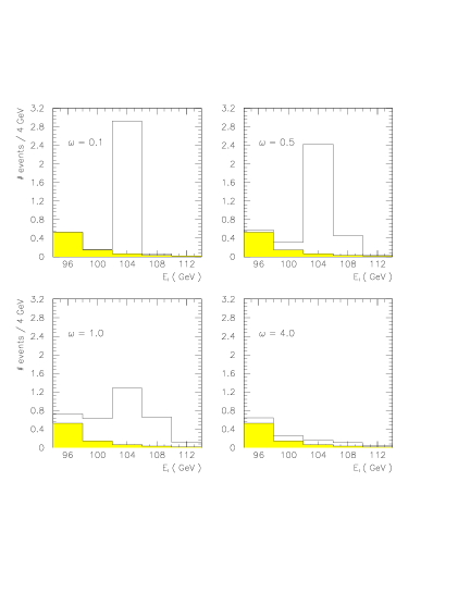
Figure 6: The event histograms belonging to Fig. (5) assuming an integrated luminosity of $300pb^{-1}$. The background is shaded.

To illustrate the dependence of the event rates and cross sections for invisible Higgs decay on the non standard coupling $\omega$ we give the expected number of signal and background events for beam energies of $\sqrt{s}=175,\,192,\,205$ GeV in the following. It should be noted, that the background is dominated by the resonating $Z^{*}$–conversion graph. It is considerably reduced by cutting away the energy region, where the cross section of the resonating $Z^{*}$ is big. This should be possible, as long as the Higgs peak is sharp and well separated from the $Z^{*}$ resonance. To define a Higgs signal for a given mass, we count only events near the resonance maximum, $M_{H}\pm\Delta$. We choose $\Delta=5\,GeV$ in the following, which corresponds to a typical detector resolution for hadronic energy at LEP. The number of events per year related to the signal $S$ and background $B$ depend on the expected luminosities:

$$S_{\Delta}(\sqrt{s},M_{H}) = L(\sqrt{s})\int\limits_{(M_{H}-\Delta)^{2}}^{(M_{H}+\Delta)^{2}}ds_{Y}\frac{d\sigma_{H}}{ds_{Y}}$$ (14)

$$B_{\Delta}(\sqrt{s},M_{H}) = L(\sqrt{s})\int\limits_{(M_{H}-\Delta)^{2}}^{(M_{H}+\Delta)^{2}}ds_{Y}\frac{d(\sigma_{Z(c)}+\sigma_{Z(a)})}{ds_{Y}}$$

The assumed LEP2 luminosities are given by L(175 GeV)=500/(pb y), L(192 GeV) = L(205 GeV) = 300/(pb y).

We list the number of events, $S$, of the $\mu\mu+E\!\!\!/$-signal in Tab. (2). Though a resolution of $4\,GeV$ for the leptonic signal is possible, we put $\Delta=10$ in the signal definition, Eqn. 14, because we do not want to loose events from a smeared Higgs resonance. To compare these numbers with the hadronic decays of the Z–boson, one simply has to multiply with $B(Z\rightarrow q\bar{q})/B(Z\rightarrow\mu\mu)\simeq 20$.

$\omega$	$S_{\Delta}(175,70)$	$S_{\Delta}(192,70)$	$S_{\Delta}(192,90)$	$S_{\Delta}(205,70)$	$S_{\Delta}(205,90)$	$S_{\Delta}(205,105)$
$B_{\Delta}$	0.1 ( 0.2)	0.1 (1.5)	4.1 (4.6)	0.1 (4.9)	4.7 (4.9)	0.4 (4.9)
.1	15.7 (15.7)	8.5 (8.5)	4.7 (4.8)	7.3 (7.3)	5.1 (5.1)	2.9 (2.9)
.5	15.4 (16.1)	8.4 (8.8)	4.8 (5.0)	7.2 (7.5)	5.2 (5.4)	3.0 (3.2)
1.0	12.4 (15.3)	6.8 (8.5)	4.1 (4.9)	5.8 (7.4)	4.4 (5.3)	2.6 (3.1)
2.0	5.5 (13.5)	3.1 (7.6)	2.1 (4.6)	2.6 (6.7)	2.4 (4.9)	1.4 (3.0)
4.0	1.5 ( 5.1)	0.8 (2.9)	0.6 (2.9)	0.7 (2.8)	0.6 (2.8)	0.4 (2.7)
8.0	0.4 ( 1.3)	0.2 (0.7)	0.1 (0.7)	0.2 (0.7)	0.2 (0.7)	0.1 (0.7)

Table 2: Number of events $S_{\Delta}$ of the $\mu\mu+E\!\!\!/$–signal at LEP2. The first line contents the background. The event rates are calculated with a cut on the missing mass of $\Delta=10$ GeV. In brackets we give the numbers without the cut.

Depending on our parameters in the $(M_{H},\omega)$–plane we present exclusion plots for several center of mass energies in Fig. (7). The $95\%$ confidence level is defined by Poisson statistics [1]. The depression for $M_{H}\sim M_{Z}$ stems from the larger background around the Z–resonance of the conversion graph. The large Higgs width leads to a restriction even for higher Higgs masses than kinematically allowed, because one probes the low energy tail of such a resonance. For a small Higgs width the bound is stronger than for a SM Higgs boson, because one can also use the hadronic decay of the $Z$–boson, as was already noticed for the LEP1 bounds above. Again the signal vanishes as the Higgs–Phion coupling is getting large.

Figure 7: Exclusion limits at LEP2 (full lines), and LEP1 (dashed). The region where $\omega$ is small is covered by the search for visible Higgs decay.

Fig. (7) reflects the fact that for a sufficiently large nonstandard coupling $\omega$, Higgs detection at LEP2 may not be possible even if it is light enough to be produced and its coupling to the Z–boson is not reduced by mixing effects. The bounds tell us the absolute size of nonperturbative effects from a light hidden sector which would forbid Higgs detection.

At the NLC the upper limits on the couplings in the present model come from the invisible decay too, as the branching ratio into visible particles drops with increasing $\varphi$–Higgs coupling ($\omega$). Because above the vector boson threshold the Higgs decay modes into SM particles are sizeable, as can be seen in Fig. (2), one has to consider visible Higgs decays, too. Since the main source for Higgs production, the $WW$–fusion process, can not be used to look for invisible Higgs decay, one is in principle left with the Higgs-Strahlung and $ZZ$–fusion reaction. For energies up to 500 GeV the Higgs-Strahlungs cross section is dominant and is of comparable size as the $ZZ$–fusion process even if one is folding in the branching ratio $B(Z\rightarrow e^{+}e^{-},\mu^{+}\mu^{-})$. The possibility to tag an on–shell Z boson via a leptonic system which is extremely useful for the discrimination of possible backgrounds makes Higgs-strahlung to be the preferred production mechanism. Thus we only have considered reactions containing an on shell Z boson with its decay into $e^{+}e^{-}$ or $\mu^{+}\mu^{-}$. One should be aware that a few events from the huge $WW$ background may survive, but that the $Z\nu\nu$ background is dominant after imposing the cuts defined below. A detailed discussion on possible backgrounds can be found in Ref. [17]. Then the signal cross section is the well known Higgs-Strahlungs cross section, Eqn. (10), modified by the non standard Higgs width due to Phion decay. We calculated the $Z\nu\nu$ background with the relevant set of graphs for Z production ($ZZ$–production, $WW$–fusion and Z initial, final state radiation) by a Monte Carlo program. The calculated amplitudes are identical to the result of Ref. [16]. To reduce the background we have used the fact that the angular distribution of the Z–boson for the signal has a peak for small values of $|\cos\theta_{Z}|$ in contrast to the background. Thus we imposed an angular cut $|\cos\theta_{Z}|<0.7$. Because we assume the reconstruction of the on–shell Z–boson we use the kinematical relation $E_{Z}=(s+M_{Z}^{2}-s_{I})/(2\sqrt{s})$ between the Z energy and the invariant mass of the invisible system to define a second cut. Since the differential cross section $d\sigma/ds_{I}$ contains the Higgs resonance at $s_{I}=M_{H}^{2}$, we impose the following condition on the Z energy

$$\frac{s+M_{Z}^{2}-(M_{H}+\Delta)^{2}}{2\sqrt{s}}<E_{Z}<\frac{s+M_{Z}^{2}-(M_{H}-\Delta)^{2}}{2\sqrt{s}}$$ (15)

which is equivalent to a cut on the invisible mass. As long as the Higgs width is small, one is allowed to use small $\Delta$, which reduces the background considerably keeping most of the signal events. But in the case of large $\varphi$–Higgs coupling, $\omega$, one looses valuable events. To compromise between both effects we took $\Delta=30$ GeV. Some cross sections are given in Tab. (3).

$\omega/M_{H}$	150	200	250	300	350	400
$B_{\Delta}$	2.51	4.73	10.01	21.44	44.85	39.10
.1	31.90	25.24	18.02	11.12	5.49	1.16
.3	31.89	25.11	17.98	11.12	5.48	1.16
.5	31.57	25.03	17.88	11.06	5.45	1.15
1.0	30.58	24.40	17.56	10.91	5.40	1.14
2.0	26.32	21.98	16.16	10.17	5.09	1.10
4.0	15.09	14.27	11.41	7.66	4.00	.93
8.0	4.61	4.85	4.32	3.22	1.88	.50
16.0	1.17	1.25	1.15	.89	.55	.16

Table 3: Cross sections of the $ee,\mu\mu,qq+E\!\!\!/$–signal at the NLC with $\sqrt{s}=500$ GeV in fb. $M_{H}$ is given in GeV. The numbers are calculated with cuts on the invisible mass, $M_{H}\pm 30$ GeV, and polar angle of the Z–boson, $|\cos(\theta_{Z})|\leq 0.7$ . The first line shows the background due to $Z\nu\nu$ reactions.

For the exclusion limits we assumed an integrated luminosity of $20\,fb^{-1}$. The result is given in Fig. 8. Again, one notices the somewhat reduced sensitivity for the mass region where $M_{H}\simeq M_{Z}$. For larger values of $M_{H}$ the limit stems from the other $Z\nu\nu$ backgrounds with $W$ bosons in the t–channel and from kinematical constraints. For large $\omega$ the signal ceases to dominate over the background because the Higgs peak is smeared out to an almost flat distribution.

Figure 8: Exclusion limits at the NLC due to Higgs searches. The dashed line corresponds to the invisible, the full line to all Higgs decay modes.

To end this section, we want to comment on invisible Higgs search at LHC. Below the two Z boson threshold the Bjorken process is the main production mechanism for Higgs bosons, too. But because of the unknown longitudinal momentum of the partons, the missing mass is not an observable. Without the possibility of reducing the background through an adequate cut, one is not able to exploit the kinematical potential of the collider. The authors of Refs. [18] give upper mass bounds for the detectability of an invisible decaying Higgs boson between 150 and 250 GeV assuming a high yearly luminosity of $100fb^{-1}$. For higher masses the cross section is simply to small. The most promising production mechanism for Higgs bosons with masses beyond the ZZ threshold, Higgs production by gluon fusion, cannot be used here due to the suppression of the branching ratio $B(H\rightarrow visible)$ in our model which is a small number in the case of strong Higgs–Phion interactions [9]. We see that the LHC is not competitive to $e^{+}e^{-}$ colliders for invisible Higgs search.

5 Conclusions

To understand and quantify the effect of light hidden matter on Higgs search at present and future colliders we introduced a scalar sector coupled to the SM Higgs sector. Explicit formulae for the modified Higgs-propagator were presented. We have shown that the main effect is that the Higgs width is becoming a free parameter. Our model is constrained by theoretical and phenomenological bounds on the parameters. First we determined the allowed region of the nonstandard couplings in respect to vacuum instability and the Landau pole by analyzing the RGEs of our model. Then we have discussed, how present experimental LEP1 data is restricting the model parameters already and how these bounds will be increased by LEP2 and NLC. We pointed out, that at LHC the presented bounds can not be extended. This is mainly because the invisible mass is not an observable. Comparing all results, we conclude that restrictive bounds on the a parameter region can be obtained by analyzing missing energy signals. But for sufficiently large coupling between the Higgs boson and the hidden sector particles the Higgs boson could escape detection, even if it is light enough to be produced. If no evidence for a SM Higgs boson occurs at these colliders, either by direct measurement of a Higgs below $\sim 700$ GeV, or through some Higgs remnant resonance in $W_{L}W_{L}$-scattering in the TeV range, strongly coupled light hidden matter could be the reason.

References

- [1] M. Carena, P.M. Zerwas (conv) et al., Higgs Physics, Proceedings of the Workshop Physics at LEP2, CERN Yellow Report 96–01.
-
[2]
OPAL Collab., D. Decamp et al., Phys. Rep. 216 (1992) 253;
OPAL Collab., preprint CERN-PPE/94-48 (1994);
DELPHI Collab., P. Abreu et. al., Nucl. Phys. B273 (1992) 3;
L3 Collab., O. Adriani et al., Phys. Lett. B303 (1993) 391;
ALEPH Collab., D. Buskulic. et al., Phys. Lett. B313 (1993) 299. -
[3]
S.L. Glashow, E.E. Jenkins, Phys. Letts. B206, (1988) 522 ;
D. Bardin, A. Leike, T. Riemann; preprint DESY 94–097. - [4] A.S. Joshipura, J.W.F. Valle, Nucl. Phys. B397, (1993) 105.
- [5] J. Ellis et. al., Phys. Rev. D39, (1989) 844.
- [6] V.A. Kuzmin, V.A. Rubakov, M.E. Shaposhnikov, Phys. Lett. B155 (1985).)
-
[7]
R.S. Chivukula, M. Golden, Phys. Lett. B267, (1991) 233;
R.S. Chivukula, M. Golden, D. Kominis, M.V. Ramana, Phys. Lett. B293, (1992) 400.
J. D. Bjorken, Int. J. Mod. Phys. A7, (1992) 4189. -
[8]
M.B. Einhorn; Nucl. Phys. B246, (1984) 75.
S. Coleman, R. Jackiw, H. D. Politzer; Phys. Rev. D10, (1974) 2491 .
L. F. Abbott, J. S. Kang, H. J. Schnitzer, Phys. Rev. 13,(1975) 2212 . - [9] T. Binoth, J.J. van der Bij, preprint Freiburg-THEP-94/26, hep–ph/9409332, proceedings of the eighth international seminar Quarks 94 (Vladimir, may 1994), 338.
- [10] J.D. Bjorken; Proc. SLAC Summer Institute (1976), SLAC Report No.198
-
[11]
M. Sher, Phys. Rep. C179, (1989) 273;
M. Lindner, Z. Phys. C31, (1986) 295. - [12] J.A. Casas, J.R. Espinosa, M. Quiros, Phys. Lett. B342, (1995) 171.
- [13] W.A. Bardeen, C.T. Hill, M. Lindner, Phys. Rev. D41, (1990) 1647.
-
[14]
R. Miquel, preprint CERN–PPE/94–70 (1994);
G. Altarelli, preprint CERN–TH.7464/94 (1994);
W. Hollik, preprint MPI–Ph/93–83 (1993). -
[15]
ALEPH Collab., D. Buskulic. et al., Phys. Letts B313,
(1993) 312;
A. Sopchak, preprint CERN–PPE/94–73 (1994). - [16] Ambrosanio S., Mele B., Nucl. Phys. B374, 3 (1992).
-
[17]
F. de Campos et. al., P.M. Zerwas (ed.),
collisions at 500 GeV:
The physics potential, Part C, DESY 93–123C, (1993) 55;
O.J.P. Éboli et al., Nucl. Phys. B421, (1994) 65. -
[18]
Choudhury D., D.P. Roy, Phys. Lett. B322, (1994) 368:
S.G. Frederikson, N. Johnson, G. Kane, J. Reid, Phys. Rev. D50, (1994) R4245;
J.F. Gunion, Phys. Rev. Lett. 72, (1994) 199.