SUSY GUTs contributions and model independent extractions of CP phases

Abstract

We consider the origin of new phases in supersymmetric grand unification model, and show how significant new contributions arise from the gluino mediated diagram. We then present a more general model independent analysis of various modes of B-decays suggested previously for measurement of the CKM phases and point out what they really measure. It is in principle possible to separate out all the phases.

We consider the origin of new CP violating phases from physics beyond the standard model (SM) and their effect on various measurements of CKM phases $\alpha$, $\beta$ and $\gamma$ proposed hitherto [1, 2, 3, 4]. Among new sources of CP violation are multi-Higgs models [5], the left-right model [6] and supersymmetry. In this note we focus on supersymmetry, which is very attractive from a grand unification viewpoint and provides many new sources of CP violation. One obvious source is the complex soft terms. Even when these are taken to be real, unification of right handed fields, like the left handed ones, can lead to a new source of CP violation. For example, a group like SO(10) [7, 8, 9] or models with intermediate gauge groups [10, 11] like $SU(2)_{L}\times SU(2)_{R}\times SU(4)_{c}$, $SU(2)_{L}\times SU(2)_{R}\times SU(3)_{c}\times U(1)_{B-L}$ have these extra phases. Supersymmetric contributions with new phases can be as large as the SM in the $B-{\bar{B}}$ mixing and loop processes that lead to $b\rightarrow s{\bar{q}}q$.

In this paper we make the first complete calculation of the gluino contribution to $\Delta m_{B}$ in a SUSY grand unified S0(10) theory. This calculation can easily be extended to the models with the intermediate gauge symmetry breaking scale considered in references [10, 11]. This calculation has been done previously by assuming same masses for the SUSY particles only for the low $\tan\beta$ scenario [8]. We consider two scenarios: (i) where the Yukawa couplings are unified (i.e. large $\tan\beta$ scenario) and (ii) a low $\tan\beta$ scenario. We show how the new contributions are large and can affect the interpretation of measurement of CKM phases. We then discuss the specific B-decay modes needed to extract the CKM phases even in the presence of new physics. This discussion actually uses model independent analysis that is valid in almost any kind of departure from the SM.

Since the soft SUSY breaking terms are gravity induced, we shall assume them to be universal at the scale $2.4\cdot 10^{18}GeV(M_{x})$ which is the reduced Plank scale. For simplicity we also assume the soft terms to be real. It has been shown that a grand unified model based on SO(10), which we will use in this paper, gives rise to flavor violating processes in both quark and lepton sectors. Consequently lepton flavor violating processes like $\mu\rightarrow e\gamma$ put bounds on the parameter space along with $b\rightarrow s\gamma$ [13]. For models with the intermediate gauge symmetry breaking scales, the soft terms can be universal even at the GUT scale and still give rise to these effects. The superpotential for the Yukawa sector at the weak scale for the SO(10) grand unification or for the grand unifying model with an intermediate scale can be written as [7, 8, 9, 11]:

$$W = Q{\bf\bar{\lambda}_{u}}{\bf U^{c}}H_{2}+Q{\bf V^{*}}{\bf\bar{\lambda}_{d}}{\bf S}^{2}{\bf V^{{\dagger}}}D^{c}H_{1}+E^{c}{\bf V_{G}^{*}}{\bf\bar{\lambda}_{L}}{\bf S}^{2}{\bf V_{G}^{{\dagger}}}LH_{1}\,,$$ (1)

where V is the CKM matrix, V_G is the CKM matrix at the GUT scale (for intermediate gauge symmetry breaking models G is replaced by I to denote the intermediate scale) and ${\bf S}$ is the diagonal phase matrix with two independent phases. The phases in the right handed mixing matrix for the down type quarks and the down type squarks can give rise to new phases in $\Delta m_{B}$ and $\Delta m_{K}$ through the gluino contribution.

The existing calculation [14] for $\Delta m_{B}$ using GUT model usually assumes that the soft terms are universal at the GUT scale($\sim 10^{16}$ GeV). Under that assumption it is found that charged Higgs has the dominant contribution. But with the universal boundary condition taken at the Planck or string scale there can be a large contribution from the gluino mediated diagram due to the fact that the fields that belong to the third generation have different masses compared to the other generation at the GUT scale due to the effect of the large top Yukawa coupling which gives rise to the non-trivial CKM like mixing matrix in the right handed sector. We first consider large $\tan\beta$ solution. In order to have a realistic fermion spectrum and the mixing parameters in the large $\tan\beta$ case, we use a maximally predictive texture developed in the reference [15]. We will look at a scenario where $\lambda_{t}(M_{G})=1$ and $\tan\beta=57.15$, which gives $m_{t}$=182 GeV and $m_{b}$=4.43 GeV. For the small $\tan\beta$ scenario we have used $\lambda_{t}(M_{G})=1.25$ and $\tan\beta=2$. Above the GUT scale we use one loop RGEs for the soft terms and the Yukawa couplings[8]. Below the GUT scale we will use the one loop RGEs in matrix form in the $3\times 3$ generation space for the Yukawa couplings and soft SUSY breaking parameters as found in Ref. [14, 16] rather than just running the eigenvalues of these matrices as is often done. Although doing this does not provide any new information when $\tan\beta$ is small, when $\tan\beta$ is large it allows one to know the relative rotation of squarks to quarks and sleptons to leptons. In the large $\tan\beta$ scenario to make sure that the electroweak symmetry is broken radiatively, we need a non zero value of the D-term usually referred as $m_{D}^{2}$, which gets introduced at the GUT scale due to the reduction of rank in the SO(10) [17]. This D-term is also bounded from above and below by requiring the pseudo scalar mass to be positive along with the squark and slepton masses[13].

We calculate $\Delta m_{B}$ using gluino contribution and compare it with the SM result. We have done the calculation in SO(10), though this calculation can easily be generalized to the models with the intermediate scale and other grand unifying models. We use the expression for $\Delta m_{K}$ given in the reference [18] (modified for the purpose of $B^{0}-{\bar{B}^{0}}$ mixing), because these expressions use the squark mass eigenstate basis derived from the full $6\times 6$ mass matrices, which automatically incorporates mixing between “right-handed” down squarks and right-handed down quarks as is inevitable with either large $\tan\beta$ or SO(10) grand unification. We plot the ratio $\Delta m_{{B}_{gluino}}$/$\Delta m_{{B}_{SM}}$ as a function of $\mu$ for different values of the gaugino masses ($m_{1/2}$) in Figure 1 for the large $\tan\beta$ case, where m₀ is 1 TeV for the entire plot. The gluino mass is related to the gaugino mass by the relation $m_{\tilde{g}}={{\alpha_{s}}\over{\alpha_{G}}}m_{1/2}$. We take $\alpha_{s}(M_{z})=0.121$ and $\alpha_{G}=1/23.9$ and the scale for grand unification to be $M_{G}=2\cdot 10^{16}$ GeV. Also in this scenario we have three variables: $m_{0}$ (the universal scalar mass), $m_{1/2}$ (the universal gaugino mass) and the $m_{D}^{2}$ (throughout our analysis we will assume the trilinear soft SUSY breaking scalar coupling $A^{0}=0$ at the Planck scale). The upper and the lower end of each curve correspond to the upper and the lower limit of the D-term respectively. As mentioned in the reference[13], the parameter space with $m_{0}$ less than 1 TeV as well as $\mu>0$ is restricted by the flavor changing neutral currents. In Figure 2 (small $\tan\beta$ case) we plot r($\equiv\Delta m_{{B}_{gluino}}$/$\Delta m_{{B}_{SM}}$) as a function of the gaugino mass ($m_{1/2}$) for different values of the scalar masses $m_{0}$, where $\tan\beta$ is assumed to be 2 and $\mu<0$. In the plot we have used the absolute value of $\Delta m_{B_{d}}$. We restrict ourselves to the parameter space allowed by the other flavor changing decays. We also make sure that $\mu$ is less than 800 GeV to avoid fine tuning. In both figures the SUSY contribution can be comparable to the SM. As a matter of fact in this parameter space the gluino contribution to the $b\rightarrow s\gamma$ is also large [12, 13]. From the graph one can see that for the scalar mass (or the right handed slepton mass) m₀=1 TeV and for the gaugino mass $m_{1\over 2}\geq 140$ GeV (or the gluino mass $\geq 405$ GeV), the SUSY contribution is small (less than 20 $\%$) compared to the SM in the large $\tan\beta$ scenario. In the low $\tan\beta$ scenario, for the gaugino mass $m_{1\over 2}\geq 200$ GeV (or the gluino mass $\geq 578$ GeV) and for the scalar mass (or the right handed slepton mass) m${}_{0}\geq 200$ GeV, the SUSY contribution becomes small (less than 20 $\%$) compared to the SM. For a complete SUSY calculation, there could be contributions from charged Higgs, chargino and neutralino. The charged Higgs contribution does not change significantly with the new boundary condition and has been found to be comparable to or even greater than the SM contribution when the soft SUSY breaking terms are taken at the GUT scale [14]. Also this contribution does not involve any right handed down type quark-squark mixing, so that it has the same phase structure as the SM does. Consequently, the CKM measurement is not affected from the charged Higgs contribution as we will discuss later. Chargino and neutralino contributions are usually small [14, 19] and have no effect on the CKM measurements.

The soft terms (e.g A and or $\mu$) can also be complex. In that case one can get phases in $\Delta m_{B}$ even without grand unification. The complex terms in the mass matrix for the squarks and sleptons are then responsible for the new phases which are somewhat restricted by the edm of electron or neutron [20], however large phases can appear when the scalar masses are in the TeV range [21]. There could also be an induced phase in A due to the phase in the Yukawa sector through renormalization, even when A is real at the GUT scale. The phase induced is really small and gives rise to the edm of electron well within the experimental limit for squarks and gluino masses O(100 GeV) [22]. It is possible to get comparable $\Delta m_{B_{d}}$ and $\Delta m_{K}$ from supersymmetric contribution with new phases [23] in a model based on the MSSM (without grand unification) with right handed mixing matrix in the up sector.

The contribution to the $\Delta m_{B_{d,s}}$ can be parameterized as :

$$\Delta m_{B_{d}} = A_{SM}+B_{SUSY}+C_{SUSY}e^{i\phi},$$ (2)

$$\Delta m_{B_{d}} = A_{B_{d}}V_{td}^{*^{2}}V_{tb}^{2}e^{i\phi_{B_{d}}}.$$ (3)

To make the analysis a most general one we have included $B_{SUSY}$ which has the same phase structure as A_SM. In our example, for $\Delta m_{B_{d}}$, the box diagram with the LRLR structure (helicities of the fermions in the external legs) has the mixing structure $\left|V_{td}\right|^{2}e^{i\phi}$, and RRRR type of box diagram has the mixing structure $V_{td}^{{}^{2}}e^{2i\phi}$ in the diagonal quark mass basis with just b squark in the loop, where $\phi$ arises from the matrix $S$. Note that even if $\phi$ is 0, both the RRRR type and LRLR type still have different phase structures compared to the SM. As a matter of fact any contribution from beyond the SM including multi-Higgs models and left-right models can be written as above. $A_{B_{d}}e^{i\phi_{B_{d}}}$ originates from the combination of the SM contribution and the new contribution. Similarly we have for $B_{s}-{\bar{B}_{s}}$ and $K-{\bar{K}}$ mixing:

$$\Delta m_{B_{s}}=A_{B_{d}}V_{ts}^{*^{2}}V_{tb}^{2}e^{i\phi_{B_{s}}},\;\Delta m_{K}=A_{K}V_{cs}^{*^{2}}V_{cd}^{2}e^{i\phi_{K}}.$$ (4)

Expressions for ${q/p}$ for each of these mesons are now:

$$\left({q\over p}\right)_{B_{d}}=\left({V_{tb}^{*}{V_{td}}\over{V_{tb}V_{td}^{*}}}\right)e^{-i\phi_{B_{d}}},\;\left({q\over p}\right)_{B_{s}}=\left({V_{tb}^{*}{V_{ts}}\over{V_{tb}V_{ts}^{*}}}\right)e^{-i\phi_{B_{s}}},\;\left({q\over p}\right)_{K}=\left({V_{cd}^{*}{V_{cs}}\over{V_{cd}V_{cs}^{*}}}\right)e^{-i\phi_{K}}.$$ (5)

In general $\phi_{B_{d}}$, $\phi_{B_{s}}$ and $\phi_{K}$ are unrelated. These phases are so defined that they are in addition to the phases present in the SM, and can be treated as separate observables. Charged Higgs mediated box diagram has $C=0$, and CKM measurements are unaltered. However, in our calculation $C$ is non-zero (the LRLR type and the RRRR type), and will affect CKM phase measurements.

The CKM phases are defined as: $\alpha=\mbox{Arg}\left(-{V^{*}_{tb}V_{td}/V_{ub}^{*}V_{ud}}\right),$ $\beta=\mbox{Arg}\left(-{V^{*}_{cb}V_{cd}/V_{tb}^{*}V_{td}}\right),$ $\gamma=\mbox{Arg}\left(-{V^{*}_{ub}V_{ud}/V_{cb}^{*}V_{cd}}\right)$. Based on the SM, many methods have been suggested for measuring these CKM phases using $B$ decays [1, 2, 3, 4]. The cleanest method involves time-dependent measurements of rate asymmetries in neutral $B$ decays to CP eigenstates [1], where one measures the time-dependent rate asymmetry $a_{f_{CP}}(t)$ which is a function of $\lambda\equiv\left({q/p}\right)_{i}\left({\bar{A}/A}\right)$, where $i$ denotes the corresponding mixing, i.e., $i=B_{d},B_{s}$, or $K$, and $A\equiv A(B^{0}\rightarrow f)$ and $\bar{A}\equiv\bar{A}(\bar{B}^{0}\rightarrow f)$ with CP eigenstate $f$.

We shall analyze the different CP eigenstates that have been suggested, and consider carefully what phases the measurements now yield. Our assumption for decay amplitudes is that, while the tree amplitudes have the SM phases, any loop process could have an additional unknown phase arising from beyond the Standard Model. Thus for penguin amplitudes we have

$${\bar{A}\over A}=\left({\bar{A}\over A}\right)_{SM}e^{i\phi_{peng}},$$ (6)

where $\phi_{peng}$ is a phase in addition to SM phase. The results of our analysis are presented in a convenient tabular form (Table I) modeled after a similar table in the SM given in [24]. Some of the modes have also been discussed in the reference [8] where only the SUSY grandunification contributions are retained. It is important to realize that with our definitions of additional phases as defined in Eqs. (4) and (6), these phases are measurable. Further, the analysis is essentially model independent, as these new phases can arise in any model beyond the SM.

In row (1) we consider $B_{d}\rightarrow\psi K_{S}$. This mode which is tree dominated has $Im\lambda$ given by:

$$Im\lambda = Im\left[\left({q\over p}\right)_{B_{d}}\left({q\over p}\right)_{K}\left({\bar{A}\over A}\right)\right]=Im\left[\left({V^{*}_{tb}V_{td}\over V_{tb}V^{*}_{td}}\right)e^{i\phi_{B_{d}}}\left({V_{cs}V^{*}_{cd}\over V^{*}_{cs}V_{cd}}\right)e^{i\phi_{K}}\left({V_{cb}V^{*}_{cs}\over V_{cb}^{*}V_{cs}}\right)\right]$$ (7)

$$= -\sin(2\beta+\phi_{B_{d}}+\phi_{K}).$$ (8)

Note that the mode $b\rightarrow c{\bar{c}}s$ has negligible penguin contribution. In the SM this measurement yields $\sin(2\beta)$. Similarly $B_{s}\rightarrow\psi\phi$, $\psi\eta$ would yield $\phi_{B_{s}}$ while in the SM there is no asymmetry. In row (2) and (4) we have pure penguin processes $b\rightarrow s{\bar{s}}s$ and $b\rightarrow d{\bar{d}}s$, respectively. These could have an additional weak phase $\phi_{peng}$ or $\phi_{peng}^{\prime}$ corresponding to each process. In row (2) the weak phases in $B_{s}$ and $B_{d}$ are the same $\phi_{peng}$ because they arise from the same quark subprocess. The processes in row (3) are generally not suitable as both tree and penguin amplitudes make comparable contributions to the final states. In row (5) tree amplitude dominates and although the modes are Cabibbo suppressed, they are useful. In row (6) it is assumed that in the SM top contribution dominates in the loop. The contributions from charm and up quarks are expected to be about 10% over most of the allowed range [25]. In row (7) tree contribution dominates and the small penguin admixture can be removed using isospin analysis [2]. Row (8) has processes dominated by tree diagrams and even though the mode $D^{0}K^{*}$ is not a CP eigenstate, an analysis of this mode can be used to determine $\gamma$ [3]. The charged $B$ decay mode $D^{0}K^{+}$ can be used alternatively, based on the same type of analysis [4].

It is clear from the table I that from $B_{d}$ decays we can extract the combination $\beta+\phi_{B_{d}}/2$ and $\phi_{K}$, $\phi_{peng}$ and $\gamma$. From $B_{s}$ decays it is possible to measure $\phi_{B_{s}}$, $\phi_{K}$, $\phi_{peng}$, $\phi_{peng}^{\prime}$ and $\gamma$ and the combination $\beta+\phi_{peng}^{\prime\prime}/2$. However, combining both measurements, it is possible in principle to extract all phases separately. Thus $\beta$ and $\gamma$ are determined and $\alpha$ can be solved for. Since all the measurements involve $sine$ of some angle, there exists some ambiguity in determination of a definite angle. However the analysis involved in the process $D^{0}K^{*}(892)$ is in principle expected to determine the definite value $\gamma$, if in addition one studies the exclusive processes $B_{d}\rightarrow D^{0}X^{0}$ ($X^{0}$ is $K^{+}\pi^{-}$, $K^{+}\pi^{-}\pi^{0}$, etc.) to remove discrete ambiguity [3].

We recall that in the SM with three generations, the sum of three CKM phases $\alpha$, $\beta$ and $\gamma$ must be equal to $\pi$. In order to check the validity of this unique feature, one would measure the CKM phases, for instance, through $B_{d}$ decay modes such as $\pi\pi$, $\psi K_{S}$ and $D^{0}K^{*}$(892) which are preferred experimentally and would yield $\alpha$, $\beta$ and $\gamma$, respectively, in the SM. However, as we can see from Table I, these modes would actually measure $\pi-(\beta+\gamma+\phi_{B_{d}}/2)$, $\beta+(\phi_{B_{d}}+\phi_{K})/2$ and $\gamma$, respectively. The sum of these three angles would give $\pi+\phi_{K}/2$ which can be a good indication for new physics unless $\phi_{K}$ turns out to be small. Even in case the experiments show the sum of these angles to be $\pi$, there is still room left for extra physics because of the possible existence of $\phi_{B_{d}}$ or $\phi_{B_{s}}$. Another interesting case is of multi-Higgs models, where SM phases might be absent. This corresponds to $\gamma=\beta=0$, $\alpha=\pi$. In that case, asymmetry in $B_{d}\rightarrow\psi K_{s}$ is opposite in sign to $B_{d}\rightarrow\pi\pi$, and $\gamma$ measurement will yield 0.

If we concentrate just on the $B_{d}$ decay modes, since these decay modes are more preferable from the experimental viewpoint, it is hard to extract all the CKM angles cleanly. But the angle $\gamma$ can still be measured without contamination of the extra phases. Since it seems to be very difficult to extract $\alpha$ and $\beta$ by using any $independent$ methods, we suggest that $\alpha$ and $\beta$ be determined using the unitarity triangle. Measuring the ratio of the CKM factors $|V_{ud}V_{ub}|/|V_{cd}V_{cb}|$ (e.g. by studying the spectra of charged leptons in the semileptonic processes $b\rightarrow u\bar{\nu}_{e}e$ and $b\rightarrow c\bar{\nu}_{e}e$) and using $\gamma$ when measured, one can construct the unitarity triangle completely, which enables one to determine the phases $\alpha$ and $\beta$ simultaneously. This angle $\beta$ should be compared with the angle measured in the $B_{d}$ decay modes such as $\psi K_{S}$ in order to extract information about new physics.

In conclusion, we have shown how the measurement of CKM phases as well as additional phases can be achieved when comparable contributions from beyond the standard model might be present.

This work was supported by Department of Energy grant DE-FG03-96ER 40969.

TABLE I.: $B$ decay modes for measuring CP angles.

	Quark Process	$B_{d}$ Modes	$B_{d}$ Angles	$B_{s}$ Modes	$B_{s}$ Angles
(1)	$b\rightarrow c\bar{c}s$	$\psi K_{S}$	$\beta+(\phi_{B_{d}}+\phi_{K})/2$	$\psi\eta$, $\psi\phi$,	$\phi_{B_{s}}/2$
				$D^{+}_{s}D^{-}_{s}$
(2)	$b\rightarrow s\bar{s}s$	$\phi K_{S}$	$\beta+(\phi_{B_{d}}+\phi_{K}+\phi_{peng})/2$	$\phi\eta$	$(\phi_{B_{s}}+\phi_{peng})/2$
(3)	$b\rightarrow u\bar{u}s$	$\pi^{0}K_{S}$, $\rho^{0}K_{S}$	$-$	$\phi\pi^{0}$, $K^{+}K^{-}$	$-$
(4)	$b\rightarrow d\bar{d}s$	$\pi^{0}K_{S}$, $\rho^{0}K_{S}$	$-$	$K^{0}\bar{K}^{0}$	$(\phi_{B_{s}}+\phi^{\prime}_{peng})/2$
(5)	$b\rightarrow c\bar{c}d$	$D^{+}D^{-}$, $\psi\pi^{0}$,	$\beta+\phi_{B_{d}}/2$	$\psi K_{S}$	$(\phi_{B_{s}}+\phi_{K})/2$
		$D^{0}\bar{D}^{0}$
(6)	$b\rightarrow s\bar{s}d$	$K^{0}\bar{K}^{0}$	$(\phi_{B_{d}}+\phi^{\prime\prime}_{peng})/2$	$\phi K_{S}$	$\beta+(\phi_{K}+\phi_{B_{s}}+\phi^{\prime\prime}_{peng})/2$
(7)	$b\rightarrow u\bar{u}d$,	$\pi\pi$, $\pi\rho$,	$\pi-(\beta+\gamma+\phi_{B_{d}}/2)$	$\rho^{0}K_{S}$, $\pi^{0}K_{S}$	$\gamma+(\phi_{B_{s}}+\phi_{K})/2$
	$d\bar{d}d$	$\pi a_{1}$
(8)	$b\rightarrow c\bar{u}s$,	$D^{0}_{CP}K^{*}$(892)	$\gamma$	$D^{0}_{CP}\phi$	$-$
	$u\bar{c}s$	$(D^{0}_{CP}K^{+})$

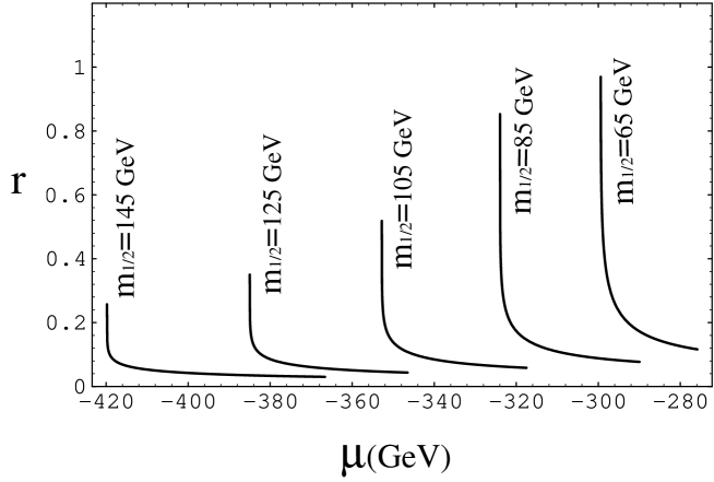
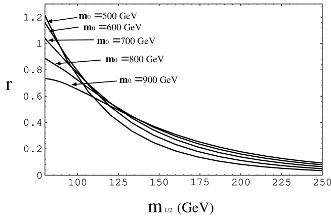
FIG. 1.: Plots of r($\equiv\Delta m_{{B}_{gluino}}$/$\Delta m_{{B}_{SM}})$ as a function of $\mu$ for different values of the gaugino masses ($m_{1/2}$). The scalar mass $m_{0}$=1 TeV for the entire plot.

FIG. 2.: Plots of r($\equiv\Delta m_{{B}_{gluino}}$/$\Delta m_{{B}_{SM}}$) as a function of the gaugino mass ($m_{1/2}$) for different values of the scalar masses $m_{0}$.

REFERENCES

- [1] For a review see, Y. Nir and H.R. Quinn, in , edited by S. Stone, p.520 (World Scientific, Singapore, 2nd ed., 1994); I. Dunietz, , p.550; A.J. Buras, Nuclear Instr. and Methods A368, 1 (1995); M. Gronau, , 21, and references therein; N.G. Deshpande, X.-G. He, Phys. Rev. Lett. 75, 3064 (1995); M. Gronau and J. Rosner, Phys. Rev. Lett. 76, 1200 (1996).
- [2] M. Gronau and D. London, Phys. Rev. Lett. 65, 3381 (1990).
- [3] I. Dunietz, Phys. Lett. B270, 75 (1991).
- [4] M. Gronau and D. Wyler, Phys. Lett. B265, 172 (1991).
- [5] T. D. Lee, Phys. Rev. D8, 1226 (1973); P. Sikivie, Phys. Lett. B65, 141 (1976); A. B. Lahanas and C. E. Vayonakis, Phys. ReV. D19, 2158 (1979); Y. L. Wu, L. Wolfenstein, Phys. Rev. Lett. 73, 1762 (1994); N.G. Deshpande, X.-G. He, Phys. Rev. D49, 4812 (1994).
- [6] G. Ecker and W. Grimus, Z. Phys. C30, (1986) 293; D. London and D. Wyler, Phys. Lett. B232, (1989) 503.
- [7] S. Dimopoulos and L. J. Hall, Phys. Lett. B344, 185 (1995).
- [8] R. Barbieri, L. J. Hall, and A. Strumia, Nucl. Phys. B449, 437 (1995).
- [9] R. Barbieri, L. J. Hall, and A. Strumia, Nucl. Phys. B445, 219 (1995).
- [10] N.G. Deshpande, B. Dutta, E. Keith, Phys. Rev. D54, 730 (1996).
- [11] N. G. Deshpande, B. Dutta, and E. Keith, hep-ph/9605386 (to appear in Phys. Lett. B).
- [12] B. Dutta and E. Keith, Phys. Rev. D52, 6336 (1995).
- [13] T. V. Duong, B. Dutta and E. Keith, Phys. Lett. B 378, 128 (1996).
- [14] S. Bertolini, F. Borzumati, A. Masiero, and G. Ridolfi, Nucl. Phys. B353, 591 (1991).
- [15] G. Anderson, S. Dimopoulos, L. Hall, S. Raby and G. Starkman. Phys. Rev. D49, 3660 (1994).
- [16] V. Barger, M. Berger, and P. Ohmann, Phys. Rev. D49, 4908 (1994).
- [17] A. Faraggi, J. S. Hagelin, S. Kelley and D. V. Nanopoulos, Phys. Rev. D45, 3272 (1992).
- [18] J.M. Gerard, W. Grimus, A. Raychaudhuri, G. Zoupanos, Phys. Lett. B140, 349 (1984).
- [19] G. Couture and H. Konig, Z. Phys. C69, 499 (1996); hep-ph/9511234.
- [20] J. Ellis, S. Ferrara, and D.V. Nanopoulos, Phys. Lett. 114B, (1982) 231; W. Buchmüller and D. Wyler, Phys. Lett. 121B, (1983) 321; J. Polchinski and M. Wise, Phys. Lett. 125B, (1983) 393; F. del Aguila, M. Gavela, J. Grifols, and A. Mendez, Phys. Lett. 126B, (1983) 71; D.V. Nanopoulos and M. Srednicki, Phys. Lett. 128B, (1983) 61; M. Dugan, B. Grinstein & L. Hall, Nucl. Phys. B255, 413 (1985).
- [21] Y. Kizukuri and N. Oshimo, Phys. Rev. D45, (1992) 1806; D46, (1992) 3025.
- [22] S. Bertolini, F. Vissani, Phys. Lett.B324, 164 (1994).
- [23] M. P. Worah, Phys. Rev. D54, 2198 (1996).
- [24] See article by H.R. Quinn, p.512, Particle Data Group, Phys. Rev. D50, (1996).
- [25] A.J. Buras and R. Fleischer, Phys. Lett. B341, 379 (1995).