UWThPh-1996-34

June 1996

CHIRAL PERTURBATION THEORY

Gerhard Ecker

Institut für Theoretische Physik, Universität Wien

Boltzmanngasse 5, A–1090 Wien, Austria

ABSTRACT

After a general introduction to the structure of effective field theories, the main ingredients of chiral perturbation theory are reviewed. Applications include the light quark mass ratios and pion–pion scattering to two–loop accuracy. In the pion–nucleon system, the linear $\sigma$ model is contrasted with chiral perturbation theory. The heavy–nucleon expansion is used to construct the effective pion–nucleon Lagrangian to third order in the low–energy expansion, with applications to nucleon Compton scattering.

Lectures given at the

V^th Workshop on Hadron Physics, Angra dos Reis, RJ, Brazil

April 15 - 20, 1996

To appear in the Proceedings

1 The Standard Model at Low Energies

These lecture notes consist of three parts. In the first lecture, some basic properties of chiral perturbation theory (CHPT) [1, 2, 3, 4] are reviewed. After a general classification of effective field theories, the nonlinear realization of spontaneously broken chiral symmetry is discussed. Effective chiral Lagrangians and the loop expansion are described as the two main ingredients of a systematic low–energy expansion. In the second lecture I discuss some applications in the purely mesonic sector. After a brief introduction to the phenomenology at next–to–leading order, I concentrate on our present knowledge of the light quark masses and on recent calculations of elastic $\pi\pi$ scattering to $O(p^{6})$, i.e. up to two loops. In the last lecture, nucleons and pions are treated together. The linear $\sigma$ model is contrasted with CHPT. The heavy–nucleon expansion is introduced to construct the effective pion–nucleon Lagrangian to third order in the low–energy expansion. As an instructive application, some aspects of nucleon Compton scattering are considered at the end. More extended treatments of CHPT can be found in recent reviews [5, 6, 7, 8].

1.1 Effective field theories

Effective field theories incorporate our intuitive knowledge that quantum gravity is irrelevant for understanding the pion–pion scattering phase shifts. They are the down–to–earth alternative to the Theory of Everything and they provide a theoretical framework for most of particle physics and for other fields as well. The notion of an effective theory comes with an energy scale $\Lambda$ that separates the regimes of effective and “fundamental” descriptions. Whenever we do not know the underlying theory, the effective field theory approach can be used to parametrize the unknown physics at smaller distances. But even if the “fundamental” theory is known it is often unnecessary to consider all dynamical degrees of freedom at the same footing. Instead, it may be more convenient for doing phenomenology at low energies to integrate out the heavy degrees of freedom that cannot be accessed directly at the energies in question. In many cases, the structure at small distances can be transferred to the effective level by the technique of “matching”. In other cases, this is not possible, usually because perturbation theory breaks down at the transition energy. In fact, these lectures deal with such a case: QCD in the confinement regime.

It is useful to distinguish two classes of effective field theories.

i. Decoupling effective field theories

This is the standard case where nothing much is happening in the transition from the fundamental to the effective level. As the heavy degrees of freedom are integrated out, only the light degrees of freedom already present in the theory remain. In terms of the light fields, the effective Lagrangian has the general form

$${\cal L}_{\rm eff}={\cal L}_{d\leq 4}+\sum_{d>4}\frac{1}{\Lambda^{d-4}}\sum_{i_{d}}g_{i_{d}}O_{i_{d}}~{}.$$ (1.1)

The first part ${\cal L}_{d\leq 4}$ contains the potentially renormalizable terms with operator dimension $d\leq 4$: the terms with $d<4$ are called relevant and those with $d=4$ marginal operators. The second part contains the so–called irrelevant operators with $d>4$; the $g_{i_{d}}$ are dimensionless coupling constants expected to be at most of $O(1)$, and the $O_{i_{d}}$ are monomials in the light fields with operator dimension $d$. At energies much below $\Lambda$, corrections due to the nonrenormalizable parts ($d>4$) are suppressed by powers of $E/\Lambda$. However, the usual nomenclature is sometimes misleading: in many cases of interest, some of which are listed below, it is precisely the “irrelevant” part of the effective Lagrangian that contains all the interesting physics.

There are many examples of this type:

• QED for $E\ll m_{e}$ [9].

• The Fermi theory of weak interactions for $E\ll M_{W}$. In both examples, all the interest is in the irrelevant parts of the effective Lagrangian starting with $d=8$ in the Euler–Heisenberg Lagrangian and $d=6$ for the Fermi theory.

• The Standard Model itself is in all likelihood an effective field theory. In this case, we neither know the scale $\Lambda$ nor have we caught any glimpse of the interesting “irrelevant” part yet.

• The scattering of light on neutral atoms for small photon energies can also be treated with an effective field theory. I refer to Ref. [10] for an explanation in field theory terms of why the sky is blue.

ii. Non–decoupling effective field theories

In this second case, the transition from the fundamental to the effective level occurs through a phase transition via the spontaneous breakdown of a symmetry generating Goldstone bosons that usually acquire a small mass ($M\ll\Lambda$) due to some explicit symmetry breaking (pseudo–Goldstone bosons). A spontaneously broken symmetry relates processes with different numbers of Goldstone bosons. Such a symmetry transformation is therefore nonlinear in the Goldstone fields and the distinction between renormalizable ($d\leq 4$) and nonrenormalizable ($d>4$) parts in the effective Lagrangian (1.1) would not be preserved under a symmetry transformation. There is no intrinsic difference between relevant, marginal and irrelevant operators in this case. Although we shall encounter a well–known exception in the form of the linear $\sigma$ model [11], the effective Lagrangian in the non–decoupling case is generically nonrenormalizable.

The Goldstone theorem [12] does not only predict the existence of massless excitations, but it also requires that the interactions of Goldstone bosons vanish as their energies tend to zero. This is the basis for a systematic low–energy expansion of effective Lagrangians of type ii: instead of the operator dimension as in (1.1), the number of derivatives (powers of momenta in momentum space) distinguishes successive terms in the Lagrangian.

The general structure of effective Lagrangians with spontaneously broken symmetries is largely independent of the specific physical realization. Two well–known examples in particle physics are the Standard Model without an explicit Higgs boson (heavy–Higgs scenario) where a gauge symmetry is spontaneously broken and QCD at energies below 1 GeV where the global chiral symmetry is spontaneously broken. The universality of Goldstone boson interactions implies that the scattering of longitudinal gauge vector bosons is in first approximation analogous to $\pi\pi$ scattering. The comparison between these two examples may carry an additional message. The Higgs sector of the Standard Model is modelled after the linear $\sigma$ model of low–energy hadron physics. As I will explain in the third lecture, we now know that the linear $\sigma$ model is not the effective field theory for QCD. The realistic effective field theory at low energies (CHPT) can do without an explicit scalar field. Could this be a lesson for the scalar sector at the Fermi scale?

1.2 Chiral symmetry

QCD with $N_{f}$ massless quarks exhibits a global symmetry

$$\underbrace{SU(N_{f})_{L}\times SU(N_{f})_{R}}_{\mbox{chiral group $G$}}\times U(1)_{V}\times U(1)_{A}~{}.$$

At the effective hadronic level, the quark number symmetry $U(1)_{V}$ is realized as baryon number. The axial $U(1)_{A}$ is not a symmetry at the quantum level due to the Abelian anomaly [13].

A classical symmetry can be realized in quantum field theory in two different ways depending on how the vacuum responds to a symmetry transformation (Wigner–Weyl vs. Nambu–Goldstone). There is a large body of theoretical and phenomenological evidence that the chiral group $G$ is spontaneously broken to the vectorial subgroup $H=SU(N_{f})_{V}$ [isospin for $N_{f}=2$, flavour $SU(3)$ for $N_{f}=3$]. The axial generators of $G$ are nonlinearly realized and there are $N_{f}^{2}-1$ massless pseudoscalar Goldstone bosons to be identified with the low–lying pseudoscalar mesons.

Spontaneous symmetry breaking $G\to H$ can be characterized by one or more order parameters. In quantum field theory, they take the form of vacuum expectation values

$$\langle 0|A|0\rangle$$ (1.2)

of operators $A$ that are invariant under the conserved subgroup $H$ but transform non–trivially under the full group $G$. If the vev (1.2) is non–vanishing, the vacuum cannot be invariant under $G$ signalling spontaneous symmetry breaking. Which are the possible order parameters for chiral symmetry breaking in QCD? The operators $A$ must be Lorentz scalar (even parity), colour singlet, $G$ non–invariant, but $SU(N_{f})_{V}$ invariant quark–gluon operators. Ordering the candidate operators according to their dimension, one finds a unique possibility with the smallest possible dimension $d=3$: $A={\overline{q}}q$ where $q=u,d(,s)$ for $N_{f}=2(3)$. The order parameters are called quark condensates:

$$\langle 0|{\overline{u}}u|0\rangle=\langle 0|{\overline{d}}d|0\rangle(=\langle 0|{\overline{s}}s|0\rangle)\neq 0~{}.$$ (1.3)

The equalities in (1.3) are a consequence of $SU(N_{f})_{V}$ invariance. Increasing the dimension, there is again a unique operator with $d=4$, the square of the gluon field strength that is however a $G$ singlet and therefore not relevant for an order parameter. Also for $d=5$, there is a single candidate ${\overline{q}}\lambda^{a}\sigma_{\mu\nu}G_{a}^{\mu\nu}q$ giving rise to the so–called mixed condensate. For $d\geq 6$, there are many more possibilities such as four–quark operators.

The original formulation of CHPT [2, 3] assumes that the quark condensates have the values extracted from many different applications of QCD sum rules [14] but also from lattice simulations [15], giving rise to the dominant contributions for the masses of the pseudoscalar mesons. These lectures deal with the standard formulation of CHPT. In the not very likely case that all the sum rule and lattice evidence is misleading and the quark condensates are much smaller or even zero, an alternative framework called Generalized CHPT [16] might become more appropriate. Occasionally, I will come back to this option.

There is a standard procedure how to implement a symmetry transformation on the Goldstone fields [17]. Geometrically, the Goldstone fields $\varphi$ can be viewed as coordinates of the coset space $G/H$. An element $g$ of the symmetry group $G$ induces in a natural way (by left translation) a transformation of $u(\varphi)\in G/H$:

$$u(\varphi)\stackrel{{\scriptstyle G}}{{\to}}gu(\varphi)=u(\varphi^{\prime})h(g,\varphi)~{}.$$ (1.4)

The so–called compensator field $h(g,\varphi)$ is an element of the conserved subgroup $H$ and it accounts for the fact that a coset element is only defined up to an $H$ transformation. For $g\in H$, the symmetry is realized in the usual linear way (Wigner–Weyl) and $h(g)$ does not depend on the Goldstone fields $\varphi$. On the other hand, for $g\in G$ corresponding to a spontaneously broken symmetry ($g\not\in H$), the symmetry is realized nonlinearly (Nambu–Goldstone) and $h(g,\varphi)$ does depend on $\varphi$.

For the special case of chiral symmetry $G=SU(N_{f})_{L}\times SU(N_{f})_{R}$, parity relates left– and right–chiral transformations. With a standard choice of coset representatives the general transformation (1.4) then takes the special form

$$u(\varphi^{\prime})=g_{R}u(\varphi)h(g,\varphi)^{-1}=h(g,\varphi)u(\varphi)g_{L}^{-1}$$ (1.5)

$$g=(g_{L},g_{R})\in G~{}.$$

Since the chiral coset space $SU(N_{f})_{L}\times SU(N_{f})_{R}/SU(N_{f})_{V}$, even though it is not a group, is homeomorphic to $SU(N_{f})$ as a manifold, $u(\varphi)\in SU(N_{f})$ is a matrix–valued field. Different forms (the most familiar one being the exponential parametrization) correspond to different coordinate systems. A field transformation amounts to a coordinate transformation in coset space.

For practical purposes, one never needs to know the explicit form of $h(g,\varphi)$, but only the transformation property (1.5). In the mesonic sector, it is often more convenient to work with the square of $u(\varphi)$. Because of (1.5), the matrix field $U(\varphi)=u(\varphi)^{2}$ has a simpler linear transformation behaviour:

$$U(\varphi)\stackrel{{\scriptstyle G}}{{\to}}g_{R}U(\varphi)g_{L}^{-1}~{}.$$ (1.6)

It is therefore frequently used as basic building block for chiral Lagrangians. When non–Goldstone degrees of freedom like baryons or meson resonances are included in the effective Lagrangians, the nonlinear picture with $u(\varphi)$ and $h(g,\varphi)$ is more appropriate. In the third part of these lectures, the abstract quantities introduced here will emerge naturally when we investigate the linear $\sigma$ model in some detail.

Before embarking on the construction of effective chiral Lagrangians, we recall that there is actually no chiral symmetry in nature. In addition to the spontaneous breaking, chiral symmetry is explicitly broken both by non–vanishing quark masses and by the electroweak interactions. Both conceptually and for practical purposes, the best way to keep track of the explicit breaking is through the introduction of external matrix fields [2, 3] $v,a,s,p$. The QCD Lagrangian ${\cal L}^{0}_{\rm QCD}$ for massless quarks is extended to

$${\cal L}={\cal L}^{0}_{\rm QCD}+\bar{q}\gamma^{\mu}(v_{\mu}+a_{\mu}\gamma_{5})q-\bar{q}(s-ip\gamma_{5})q$$ (1.7)

to include electroweak interactions of quarks with external gauge fields $v,a$ and to allow for nonzero quark masses by setting the scalar matrix field $s(x)$ equal to the diagonal quark mass matrix. One performs all calculations with a (locally) $G$ invariant effective Lagrangian in a manifestly chiral invariant manner. Only at the very end, one inserts the appropriate external fields to extract the Green functions of quark currents or matrix elements of interest. The explicit breaking of chiral symmetry is automatically taken care of by this spurion technique. In addition, electromagnetic gauge invariance is manifest. All Ward identities for Green functions of quark currents are guaranteed.

Although this procedure produces all Green functions for electromagnetic and weak currents, the method must be extended in order to include virtual photons (electromagnetic corrections) or virtual $W$ bosons (nonleptonic weak interactions).

1.3 Chiral Lagrangians

CHPT is based on a two–fold expansion. As a low–energy effective field theory, it is an expansion in small momenta. On the other hand, it is also an expansion in quark masses around the chiral limit. In full generality, the effective chiral Lagrangian is of the form

$${\cal L}_{\rm eff}=\sum_{i,j}{\cal L}_{ij}~{},\qquad\qquad{\cal L}_{ij}=O(p^{i}m^{j}_{q})~{}.$$ (1.8)

The two expansions become related by expressing the pseudoscalar meson masses in terms of the quark masses $m_{q}$. If the quark condensate is non–vanishing in the chiral limit, the squares of the meson masses start out linear in $m_{q}$ [cf. Eq. (1.12)]. Assuming the linear terms to give the dominant contributions to the meson masses, one arrives at the standard chiral counting [2, 3] with $m_{q}=O(p^{2})$ and

$${\cal L}_{\rm eff}=\sum_{d}{\cal L}_{d}~{},\qquad\qquad{\cal L}_{d}=\sum_{i+2j=d}{\cal L}_{ij}~{}.$$ (1.9)

As already mentioned, there are many indications in favour of the standard picture. In addition to QCD sum rules and lattice simulations, the Gell-Mann–Okubo mass formula (1.15) for the pseudoscalar meson masses can only be understood in a natural way if the squares of the meson masses are linear in the quark masses to a good approximation. In order to account for the logical possibility that the quark condensate would not give the main contributions to the meson masses, the proponents of Generalized CHPT [16] suggest a reordering of the effective Lagrangian. Through this reordering, more terms appear at a given order that are relegated to higher orders in the standard counting. Therefore, more unknown constants appear at any given order compared to the standard framework. Nevertheless, the effective chiral Lagrangian is the same in both approaches. In these lectures, I will adhere to the standard procedure, but I will refer once more to Generalized CHPT when discussing $\pi\pi$ scattering at the two–loop level.

The construction of the effective chiral Lagrangian for the strong interactions of mesons is now straightforward. In terms of the basic building blocks $U(\varphi)$ and the external fields $r_{\mu}=v_{\mu}+a_{\mu}$, $l_{\mu}=v_{\mu}-a_{\mu}$, $s$ and $p$ and with the standard chiral counting just described, the chiral invariant Lagrangian starts out at $O(p^{2})$ with

$${\cal L}_{2}=\frac{F^{2}}{4}\langle D_{\mu}UD^{\mu}U^{\dagger}+\chi U^{\dagger}+\chi^{\dagger}U\rangle$$ (1.10)

$$\chi=2B(s+ip)\qquad\qquad D_{\mu}U=\partial_{\mu}U-ir_{\mu}U+iUl_{\mu}$$

where $\langle\dots\rangle$ stands for the $N_{f}-$dimensional trace. The two low–energy constants (LECs) at $O(p^{2})$ are related to the pion decay constant and to the quark condensate in the chiral limit:

$$F_{\pi}=F[1+O(m_{q})]=92.4~{}{\rm MeV}$$ (1.11)

$$\langle 0|\bar{u}u|0\rangle=-F^{2}B[1+O(m_{q})]~{}.$$

Expanding the Lagrangian (1.10) to second order in the meson fields and setting the external scalar field equal to the quark mass matrix, one can immediately read off the pseudoscalar meson masses to leading order in $m_{q}$, e.g.,

$$M^{2}_{\pi^{+}}=(m_{u}+m_{d})B~{}.$$ (1.12)

As expected, the squares of the meson masses are linear in the quark masses to leading order if the quark condensate is non–vanishing in the chiral limit ($B\neq 0$). The full set of equations for the masses of the pseudoscalar octet gives rise to several well–known relations:

$$F_{\pi}^{2}M_{\pi}^{2}=-(m_{u}+m_{d})\langle 0|\bar{u}u|0\rangle$$ [18] (1.13)

$$B=\frac{M_{\pi}^{2}}{m_{u}+m_{d}}=\frac{M_{K^{+}}^{2}}{m_{s}+m_{u}}=\frac{M_{K^{0}}^{2}}{m_{s}+m_{d}}$$ [19] (1.14)

$$3M^{2}_{\eta_{8}}=4M_{K}^{2}-M_{\pi}^{2} \cite[cite]{[\@@bibref{}{GMO57}{}{}]}.$$ (1.15)

The effective chiral Lagrangian of the Standard Model is shown schematically in Table 1. The subscripts of the different parts of this Lagrangian denote the chiral dimension according to the standard counting and the numbers in brackets indicate the appropriate number of LECs. The notation even/odd refers to the mesonic Lagrangians without/with an $\varepsilon$ tensor (even/odd intrinsic parity). For instance, ${\cal L}_{4}^{\rm odd}(0)$ stands for the anomalous Lagrangian of the Wess–Zumino–Witten functional [21] that has no free parameters. I have grouped together those pieces of the Lagrangian that have the same chiral order as a corresponding loop amplitude ($L$ = 0, 1, 2). For a given $L$, the first line contains purely mesonic Lagrangians and the second one refers to the pion–nucleon system. The Lagrangians ${\cal L}_{n}^{\Delta S=1}$ and ${\cal L}_{n}^{\gamma}$ describe nonleptonic weak interactions and virtual photons, respectively. There are similar Lagrangians for the meson–baryon system which I have not included in the Table. In the meson–baryon sector only the pion–nucleon Lagrangian is included, i.e. $N_{f}=2$. On the other hand, the numbers of LECs in the purely mesonic Lagrangians are given for $N_{f}=3$. The theory has to be renormalized for $L\geq 1$. The parts of the effective chiral Lagrangian that have been completely renormalized are underlined in Table 1.

Table 1: The effective chiral Lagrangian of the Standard Model

${\cal L}_{\rm chiral\,\,dimension}$  ($\#$ of LECs)		loop order
${\cal L}_{2}(2)$ + ${\cal L}_{4}^{\rm odd}(0)$ + ${\cal L}_{2}^{\Delta S=1}(2)$  + ${\cal L}_{0}^{\gamma}(1)$		$L=0$
+ ${\cal L}_{1}^{\pi N}(1)$ + ${\cal L}_{2}^{\pi N}(7)$ + …
+ $\underline{{\cal L}_{4}^{\rm even}(10)}$ + $\underline{{\cal L}_{6}^{\rm odd}(32)}$  + $\underline{{\cal L}_{4}^{\Delta S=1}(22,{\rm octet})}$ +  $\underline{{\cal L}_{2}^{\gamma}(14)}$		$L=1$
+ $\underline{{\cal L}_{3}^{\pi N}(24)}$ + ${\cal L}_{4}^{\pi N}(?)$ + …
+ ${\cal L}_{6}^{\rm even}(111)$ + …		$L=2$

Why do we have to add special Lagrangians for the nonleptonic weak interactions and for virtual photons? After all, the strong chiral Lagrangian like (1.10) contains external photons and $W$ bosons. However, unlike for semileptonic processes where we can hook on a leptonic current (electromagnetic or weak) to the external gauge fields, the strong interactions cannot be disentangled from the electroweak interactions in the nonleptonic case. Put in another way, Green functions of quark currents are not sufficient to generate nonleptonic weak amplitudes or amplitudes with virtual photons.

Let us first consider the nonleptonic weak interactions. At the low energies relevant for CHPT, the correct procedure is to first integrate out the $W$ together with the heavy quarks to arrive at an effective Hamiltonian already at the quark level [22, 23]:

$${\cal H}_{\rm eff}^{\Delta S=1}=\frac{G_{F}}{\sqrt{2}}V_{ud}V_{us}^{*}\sum_{i}C_{i}(\mu)Q_{i}+{\rm h.c.}$$ (1.16)

The $C_{i}(\mu)$ are Wilson coefficients depending on the QCD renormalization scale $\mu$. The $Q_{i}$ are local four–quark operators if we limit the operator product expansion (1.16) to the leading $d=6$ operators. For the effective realization at the hadronic level, the explicit form of the $Q_{i}$ (or of the Wilson coefficients) is of no concern. All that is needed is the transformation property of ${\cal H}_{\rm eff}^{\Delta S=1}$ under chiral rotations:

$${\cal H}_{\rm eff}^{\Delta S=1}\sim(8_{L},1_{R})+(27_{L},1_{R})~{}.$$ (1.17)

The task is then to construct the most general chiral Lagrangian that has the same transformation property (1.17) under chiral transformations. As indicated in Table 1, the lowest–order Lagrangian is again of $O(p^{2})$ and it has two LECs, one for the octet piece and one for the 27–plet.

Integrating out the photons cannot be described by a local operator at low energies as in the case of the massive $W$ boson. In a first step, the electromagnetic field is made dynamical by including the appropriate kinetic term and by enlarging the external vector field $v_{\mu}$:

$$v_{\mu}\rightarrow v_{\mu}-eQA_{\mu}~{},$$ (1.18)

where $A_{\mu}$ is the dynamical photon field and the quark charge matrix $Q$ is given in (1.20). CHPT then generates automatically all diagrams with virtual (and real) photons. However, this is not the whole story. For instance, loop diagrams with virtual photons will in general be divergent requiring appropriate local counterterms. If we restrict our attention to single–photon exchange, we must add the most general chiral Lagrangian of $O(e^{2})$ that transforms as the product of two electromagnetic currents under chiral rotations. For $N_{f}=3$, the electromagnetic current is pure octet. The easiest method for constructing the appropriate chiral Lagrangian is based on the so–called spurion technique . One writes down the most general chiral invariant Lagrangian that is bilinear in octet spurion fields $Q_{L}(x),Q_{R}(x)$ with transformation properties

$$Q_{A}(x)\stackrel{{\scriptstyle G}}{{\to}}g_{A}Q_{A}(x)g^{-1}_{A},\qquad A=L,R~{}.$$ (1.19)

Identifying the spurion fields with the quark charge matrix,

$$Q_{A}(x)=Q=\mbox{ diag}(2/3,-1/3,-1/3)~{},$$ (1.20)

gives rise to the effective chiral Lagrangian of $O(e^{2})$ with the correct transformation properties. The lowest–order Lagrangian ${\cal L}_{0}^{\gamma}(1)$ is of $O(p^{0})$ in this case and it has a single coupling constant. We will come back to this Lagrangian in the discussion of $\pi\pi$ scattering in the second lecture.

1.4 Loop expansion

Now that we know how to construct effective chiral Lagrangians we can calculate tree–level amplitudes to any desired order in the low–energy expansion. Although in the sixties many proponents of effective Lagrangians argued that due to their nonrenormalizability such Lagrangians only make sense at tree level, it is clear that tree–level amplitudes cannot be consistent with sacred principles of quantum field theory like unitarity and analyticity (except at lowest order in the chiral expansion). For instance, unitarity requires for the forward elastic meson–meson scattering amplitude $T$

$$\Im m~{}T\geq|T|^{2}~{}.$$ (1.21)

Since the (real) amplitude starts at $O(p^{2})$, there must be an imaginary part at $O(p^{4})$. This imaginary part cannot come from a hermitian Lagrangian at tree level, but can only be due to loop diagrams. Thus, the loop expansion is essential for a consistent low–energy expansion.

Today, we view effective field theories on almost the same footing as “fundamental” gauge theories (see also Ref. [24]). They admit a perfectly well–defined loop expansion although they are nonrenormalizable. The nonrenormalizability manifests itself in the appearance of additional terms that are not present in the lowest–order Lagrangian. However, ${\cal L}_{\rm eff}$ is already the most general chiral Lagrangian with the appropriate transformation properties. Since the divergences can be absorbed by local counterterms that exhibit the same symmetries as the initial Lagrangian, ${\cal L}_{\rm eff}$ automatically includes all terms needed for renormalization to every order in the loop expansion.

Before we can renormalize the theory, we have to regularize it. In principle, any regularization that respects chiral symmetry is good enough. In practice, a mass independent regularization scheme like dimensional regularization is best suited for the purpose. In addition to respecting chiral symmetry, it very much simplifies the chiral counting and it avoids spurious quadratic or higher divergences.

To keep track of the chiral counting, it is convenient to define the chiral dimension of an amplitude. In the mesonic case with only pseudoscalar mesons in internal lines, the chiral dimension $D$ of a connected $L$–loop amplitude with $N_{d}$ vertices of $O(p^{d})$ ($d=2,4,\ldots)$ is given by [1]

$$D=2L+2+\sum_{d}(d-2)N_{d}~{},\qquad d=4,6,\ldots$$ (1.22)

As this formula shows, the number $N_{2}$ of vertices from the lowest–order Lagrangian (1.10) does not affect the chiral dimension. The following classification of amplitudes with chiral dimension up to $O(p^{6})$ is therefore independent of $N_{2}$:

$$D=2: L=0$$

$$D=4: L=0, N_{4}=1$$

$$L=1$$

$$D=6: L=0, N_{6}=1$$ (1.23)

$$L=0, N_{4}=2$$

$$L=1, N_{4}=1$$

$$L=2 ~{}.$$

The basic topological structures for $D=6$ are shown in Fig. 1. In any of these diagrams arbitrary tree structures from the lowest–order Lagrangian (1.10) can emerge from both the lines and the vertices. For instance, to find all diagrams contributing to $\pi\pi$ scattering at $O(p^{6})$ one hooks on four external pion lines to every skeleton diagram in Fig. 1 in all possible allowed ways. We come back to $\pi\pi$ scattering in the second lecture.

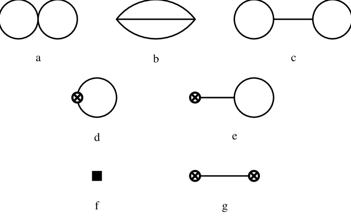
Figure 1: Skeleton diagrams of $O(p^{6})$. Normal vertices are from ${\cal L}_{2}$, crossed circles denote vertices from ${\cal L}_{4}$ and the square in diagram f stands for a vertex from ${\cal L}_{6}$. The propagators and vertices carry the full tree structure associated with the lowest–order Lagrangian ${\cal L}_{2}$.

For a given amplitude, the chiral dimension $D$ increases with $L$ according to Eq. (1.22). In order to reproduce the (fixed) physical dimension of the amplitude, each loop produces a factor $1/F^{2}$. Together with the geometric loop factor $(4\pi)^{-2}$, the loop expansion suggests

$$4\pi F_{\pi}=1.2\mbox{ GeV}$$ (1.24)

as the natural scale of the chiral expansion [25]. A more refined analysis leads to

$$4\pi F_{\pi}/\sqrt{N_{f}}$$ (1.25)

as the relevant scale for $N_{f}$ light flavours [26]. Restricting the domain of applicability of CHPT to momenta $|p|\stackrel{{\scriptstyle<}}{{{}_{\sim}}}O(M_{K})$, the natural expansion parameter of chiral amplitudes based on the naive estimate (1.24) is expected to be of the order

$$\frac{M_{K}^{2}}{16\pi^{2}F_{\pi}^{2}}=0.18~{}.$$ (1.26)

In addition, these terms often appear multiplied with chiral logarithms. It is therefore no surprise that substantial higher–order corrections in the chiral expansion are the rule rather than the exception for chiral $SU(3)$. On the other hand, for $SU(2)_{L}\times SU(2)_{R}$ and for momenta $|p|\stackrel{{\scriptstyle<}}{{{}_{\sim}}}O(M_{\pi})$ the chiral expansion is expected to converge considerably faster.

It is rather obvious that chiral invariant Lagrangians together with a chiral invariant regularization and renormalization procedure will produce amplitudes that respect all chiral Ward identities. It is expected, but highly non–trivial nevertheless, that the converse is also true. As shown by Leutwyler [4], the most general solution of chiral Ward identities can always be generated by a locally chiral invariant ${\cal L}_{\rm eff}$. The only exception is the chiral anomaly that requires a Wess–Zumino–Witten term [21], but the rest is gauge invariant (see also Ref. [27]).

2 The Physics of Mesons

2.1 Phenomenology at next–to–leading order

The Green functions and amplitudes of lowest order $p^{2}$ (current algebra level) are determined by the Lagrangian (1.10) at tree level. At next–to–leading order, $O(p^{4})$, there are three types of contributions [2, 3] in accordance with (1.23):

• Tree diagrams with a single vertex from the effective chiral Lagrangian ${\cal L}_{4}$ of $O(p^{4})$ given below and, as usual, any number of vertices from ${\cal L}_{2}$.

• One–loop diagrams with all vertices from ${\cal L}_{2}$.

• The Wess–Zumino–Witten functional [21] to account for the chiral anomaly [28].

For $N_{f}=3$, the effective chiral Lagrangian ${\cal L}_{4}(U,v,a,s,p)$ has the form [3]

$${\cal L}_{4} = L_{1}\langle D_{\mu}U^{\dagger}D^{\mu}U\rangle^{2}+L_{2}\langle D_{\mu}U^{\dagger}D_{\nu}U\rangle\langle D^{\mu}U^{\dagger}D^{\nu}U\rangle$$ (2.1)

$$+L_{3}\langle D_{\mu}U^{\dagger}D^{\mu}UD_{\nu}U^{\dagger}D^{\nu}U\rangle+L_{4}\langle D_{\mu}U^{\dagger}D^{\mu}U\rangle\langle\chi^{\dagger}U+\chi U^{\dagger}\rangle$$

$$+L_{5}\langle D_{\mu}U^{\dagger}D^{\mu}U(\chi^{\dagger}U+U^{\dagger}\chi)\rangle+L_{6}\langle\chi^{\dagger}U+\chi U^{\dagger}\rangle^{2}+L_{7}\langle\chi^{\dagger}U-\chi U^{\dagger}\rangle^{2}$$

$$+L_{8}\langle\chi^{\dagger}U\chi^{\dagger}U+\chi U^{\dagger}\chi U^{\dagger}\rangle-iL_{9}\langle F_{R}^{\mu\nu}D_{\mu}UD_{\nu}U^{\dagger}+F_{L}^{\mu\nu}D_{\mu}U^{\dagger}D_{\nu}U\rangle$$

$$+L_{10}\langle U^{\dagger}F_{R}^{\mu\nu}UF_{L\mu\nu}\rangle+L_{11}\langle F_{R\mu\nu}F_{R}^{\mu\nu}+F_{L\mu\nu}F_{L}^{\mu\nu}\rangle+L_{12}\langle\chi^{\dagger}\chi\rangle$$

where $F_{R}^{\mu\nu}$, $F_{L}^{\mu\nu}$ are the field strength tensors associated with the external gauge fields $r_{\mu}$, $l_{\mu}$. This is the most general Lorentz invariant Lagrangian of $O(p^{4})$ with local chiral symmetry, parity and charge conjugation.

Before discussing the new LECs $L_{1},\ldots,L_{12}$, let us consider one–loop diagrams. Since the theory is nonrenormalizable there are divergences all over the place. General results of renormalization theory and the chiral counting given in (1.23) ensure that those divergences can be absorbed in a local Lagrangian of $O(p^{4})$ that has all the symmetries of the lowest–order Lagrangian (1.10). But the Lagrangian (2.1) is the most general such Lagrangian. Therefore, all one–loop divergences can be absorbed by divergent LECs $L_{i}$ in (2.1). The specific values depend of course on the regularization procedure. Remember also that we are using a mass independent regularization scheme. With a mass dependent regularization, the lowest–order LECs $F$ and $B$ would in general receive quadratically divergent one–loop contributions. Since physically relevant quantities must be independent of the regularization scheme, those quadratic divergences are completely spurious effects because they do not arise in dimensional regularization for instance.

Subtracting the divergent parts of the $L_{i}$ introduces a scale dependence of the measurable LECs $L_{i}^{r}(\mu)$. This scale dependence is always compensated by the analogous scale dependence of one–loop diagrams. The latter appears in the form of so–called chiral logs $\sim\ln{p^{2}/\mu^{2}}$. The corresponding scale dependence of the LECs takes the form

$$L_{i}^{r}(\mu_{2})=L_{i}^{r}(\mu_{1})+\frac{\Gamma_{i}}{(4\pi)^{2}}\ln\frac{\mu_{1}}{\mu_{2}}~{}.$$ (2.2)

The coefficients $\Gamma_{i}$, the $\beta$–functions of the $L_{i}$, are listed in Table 2.

Table 2: Phenomenological values and source for the renormalized coupling constants $L^{r}_{i}(M_{\rho})$, taken from Ref. [29]. The quantities $\Gamma_{i}$ in the fourth column determine the scale dependence of the $L^{r}_{i}(\mu)$ according to Eq. (2.2). $L_{11}^{r}$ and $L_{12}^{r}$ are not directly accessible to experiment.

i	$L^{r}_{i}(M_{\rho})\times 10^{3}$	source	$\Gamma_{i}$
1	0.4 $\pm$ 0.3	$K_{e4},\pi\pi\rightarrow\pi\pi$	3/32
2	1.35 $\pm$ 0.3	$K_{e4},\pi\pi\rightarrow\pi\pi$	3/16
3	$-$3.5 $\pm$ 1.1	$K_{e4},\pi\pi\rightarrow\pi\pi$	0
4	$-$0.3 $\pm$ 0.5	Zweig rule	1/8
5	1.4 $\pm$ 0.5	$F_{K}:F_{\pi}$	3/8
6	$-$0.2 $\pm$ 0.3	Zweig rule	11/144
7	$-$0.4 $\pm$ 0.2	Gell-Mann–Okubo,$L_{5},L_{8}$	0
8	0.9 $\pm$ 0.3	$M_{K^{0}}-M_{K^{+}},L_{5},$	5/48
		$(2m_{s}-m_{u}-m_{d}):(m_{d}-m_{u})$
9	6.9 $\pm$ 0.7	$\langle r^{2}\rangle^{\pi}_{V}$	1/4
10	$-$5.5 $\pm$ 0.7	$\pi\rightarrow e\nu\gamma$	$-$ 1/4
11			$-$1/8
12			5/24

The renormalized coupling constants $L_{i}^{r}(\mu)$ are measurable quantities that characterize QCD at $O(p^{4})$. The present values of the $L_{i}^{r}(\mu)$ extracted from phenomenology are displayed in Table 2. Once these values are established, one can make predictions for all Green functions and amplitudes of $O(p^{4})$ in terms of the $L_{i}^{r}(\mu)$ (actually only the LECs with $i=1,\dots,10$ appear in physical quantities). This is not the place to discuss in detail the phenomenology at $O(p^{4})$ for which I refer to Refs. [5, 6, 7, 8]. By and large, the theoretical work has been completed at next–to–leading order even though experimental results are not yet available in all cases.

For reactions involving an odd number of mesons, there are no contributions at $O(p^{2})$. The leading order is $p^{4}$ and it is unambiguously given by the Wess–Zumino–Witten functional [21]. The next–to–leading order, $O(p^{6})$ in this case, involves again one–loop contributions and a Lagrangian ${\cal L}_{6}^{\rm odd}$. As indicated in Table 1, this Lagrangian has 32 new LECs. Unlike in the even–intrinsic–parity sector, most of those LECs are not yet known. One can make estimates based on meson resonance exchange, which works very well for the LECs $L_{i}$ of $O(p^{4})$ [31]. For a review of the “anomalous” sector at next–to–leading order, I refer to Ref. [32].

Let me finish this part with a remark on the structure of Green functions and amplitudes of $O(p^{4})$. Obviously, the chiral dimension $D=4$ does not imply that the relevant Green functions are just fourth–order polynomials in external momenta and masses. Instead, the chiral dimension has to do with the degree of homogeneity of the amplitudes in momenta and masses. Consider the Feynman amplitude $A$ for a general process with $D_{F}$ external photons and $W$ bosons (semileptonic transitions). If we define in addition to (1.22)

$$D=D_{L}+D_{F}~{},$$ (2.3)

then $D_{L}$ is the degree of homogeneity of the amplitude $A$ as a function of external momenta ($p$) and meson masses ($M$):

$$A(p,M;C_{i}^{r}(\mu),\mu/M)=M^{D_{L}}\,A(p/M,1;C_{i}^{r}(\mu),\mu/M)~{}.$$ (2.4)

The $C_{i}^{r}(\mu)$ denote renormalized LECs. In the meson sector at $O(p^{4})$, they are just the $L_{i}^{r}(\mu)$, but the structure (2.4) is completely general.

2.2 Light quark masses

Quark masses are fundamental parameters of QCD. The current quark masses of the QCD Lagrangian depend on the QCD renormalization scale. Since the effective chiral Lagrangians cannot depend on this scale, the quark masses always appear multiplied by quantities that transform contragrediently under changes of the renormalization scale. The chiral Lagrangian (1.9) contains the quark masses via the scalar field $\chi$ defined in (1.10). As long as one does not use direct or indirect information on $B$ [related to the quark condensates, cf. Eqs. (1.3), (1.11)], one can only extract ratios of quark masses.

The lowest–order mass formulas together with Dashen’s theorem on the lowest–order electromagnetic contributions to the meson masses [33] lead to the ratios [19]

$$\frac{m_{u}}{m_{d}}=0.55~{},\qquad\qquad\frac{m_{s}}{m_{d}}=20.1~{}.$$ (2.5)

These ratios receive higher–order corrections. The most important ones are corrections of $O(p^{4})=O(m_{q}^{2})$ and $O(e^{2}m_{s})$. The corrections of $O(p^{4})$ were worked out by Gasser and Leutwyler [3] who found that the ratios ($2\hat{m}:=m_{u}+m_{d}$)

$$\frac{M_{K}^{2}}{M_{\pi}^{2}} = \frac{m_{s}+\hat{m}}{m_{u}+m_{d}}[1+\Delta_{M}+O(m_{s}^{2})]$$ (2.6)

$$\frac{(M_{K^{0}}^{2}-M_{K^{+}}^{2})_{\rm QCD}}{M_{K}^{2}-M_{\pi}^{2}} = \frac{m_{d}-m_{u}}{m_{s}-\hat{m}}[1+\Delta_{M}+O(m_{s}^{2})]$$ (2.7)

depend on the same correction $\Delta_{M}$ of $O(m_{s})$:

$$\Delta_{M}=\frac{8(M_{K}^{2}-M_{\pi}^{2})}{F^{2}}(2L_{8}^{r}-L_{5}^{r})+\mbox{ chiral logs~{}.}$$ (2.8)

Since the ratio of these two ratios is independent of $\Delta_{M}$, one can express the quantity

$$Q^{2}:=\frac{m_{s}^{2}-\hat{m}^{2}}{m_{d}^{2}-m_{u}^{2}}$$ (2.9)

in terms of masses only, at least up to higher–order corrections:

$$Q^{2}=\frac{M_{K}^{2}}{M_{\pi}^{2}}\cdot\frac{M_{K}^{2}-M_{\pi}^{2}}{M_{K^{0}}^{2}-M_{K^{+}}^{2}+M_{\pi^{+}}^{2}-M_{\pi^{0}}^{2}}\cdot\left[1+O(m_{s}^{2})+O\left(e^{2}\frac{m_{s}}{m_{d}-m_{u}}\right)\right].$$ (2.10)

Without the corrections, this relation implies

$$Q=Q_{D}=24.2~{}.$$ (2.11)

Plotting $m_{s}/m_{d}$ versus $m_{u}/m_{d}$ leads to Leutwyler’s ellipse [34] which is to a very good approximation given by

$$\frac{1}{Q^{2}}\left(\frac{m_{s}}{m_{d}}\right)^{2}+\left(\frac{m_{u}}{m_{d}}\right)^{2}=1~{}.$$ (2.12)

In Fig. 2, the relevant quadrant of the ellipse is shown for $Q=24$ (upper curve) and $Q=21.5$ (lower curve).

Figure 2: First quadrant of Leutwyler’s ellipse [34] for $Q=24$ (upper curve) and $Q=21.5$ (lower curve). The dotted lines correspond to $\Theta_{\eta\eta^{\prime}}=-15^{0}$ (upper line) and $-25^{0}$ (lower line). The wedge between the two dashed lines corresponds to $35\leq R\leq 50$ with $R$ defined in (2.24).

However, there are possibly large corrections of $O(e^{2}m_{s})$. Assuming isospin symmetry ($m_{u}=m_{d}$), the quantity

$$\Delta_{\rm EM}=M^{2}_{K^{+}}-M^{2}_{K^{0}}-M^{2}_{\pi^{+}}+M^{2}_{\pi^{0}}$$ (2.13)

vanishes to lowest order, $O(e^{2}p^{0})$, according to Dashen’s theorem [33]. The one–loop calculation was performed independently by Urech [35] and by Neufeld and Rupertsberger [36]:

$$\Delta_{\rm EM} = -e^{2}M^{2}_{K}\left[\frac{1}{(4\pi)^{2}}\left(3\ln\frac{M^{2}_{K}}{\mu^{2}}-4+\frac{2C}{F^{4}}\ln\frac{M^{2}_{K}}{\mu^{2}}\right)+\frac{16C}{F^{4}}L_{5}^{r}(\mu)+S_{\Delta}^{r}(\mu)\right]$$ (2.14)

$$\mbox{}+O(e^{2}M^{2}_{\pi})~{}.$$

Here, $C$ is the single LEC of $O(e^{2}p^{0})$ [cf. ${\cal L}_{0}^{\gamma}(1)$ in Table 1] and $S_{\Delta}^{r}(\mu)$ is a combination of LECs of $O(e^{2}p^{2})$ corresponding to ${\cal L}_{2}^{\gamma}(14)$ in Table 1. Since $S_{\Delta}^{r}(\mu)$ is unknown, one can only calculate the scale dependent remainder without additional assumptions. The conclusion is that $\Delta_{\rm EM}$ may be sizable but the strong scale dependence precludes a more definite answer.

To get a better feeling for the size of $\Delta_{\rm EM}$, one must turn to more model dependent approaches. In Table 3 the existing predictions of different models are displayed. In summary, the earlier calculations found a rather big value while the more recent ones tend to give smaller values. The model of Ref. [37] was criticized by Baur and Urech [40] to violate chiral symmetry. The provisional overall conclusion at this time is that $\Delta_{\rm EM}$ is probably positive implying $Q<Q_{D}$ by at most 10$\%$.

Table 3: Model calculations for the quantity $\Delta_{\rm EM}$ defined in (2.13).

$\Delta_{\rm EM}\cdot 10^{3}$ GeV-2	main ingredient	Ref.
1.2	$V,A$ exchange	[37]
1.3 $\pm$ 0.4	large $N_{c}$	[38]
0.6	lattice	[39]
$-$ 0.13 $\div$ 0.36	$V,A$ exchange	[40]

There is completely independent information on $Q$ from $\eta\to 3\pi$ decays. In contrast to the masses, electromagnetic corrections are known to be tiny in this case [41, 42]. In terms of $Q$, there is a parameter free prediction for the rate to $O(p^{4})$ [43]:

$$\Gamma(\eta\to\pi^{+}\pi^{-}\pi^{0})=\Gamma_{0}\left(\displaystyle\frac{Q_{D}}{Q}\right)^{4}$$ (2.15)

with

$$\Gamma_{0}=(168\pm 50)~{}\mbox{eV}~{}.$$

The error in $\Gamma_{0}$ includes an estimate of the final state interactions. Those final state interactions have recently been calculated by two groups using dispersion relations. Both find a substantial increase of $\Gamma_{0}$:

$$\Gamma_{0}=\left\{\begin{array}[]{ll}(209\pm 20)~{}\mbox{eV}&\qquad\cite[cite]{[\@@bibref{}{KWW96}{}{}]}\\ (219\pm 22)~{}\mbox{eV}&\qquad\cite[cite]{[\@@bibref{}{AL96}{}{}]}\end{array}\right.~{}.$$ (2.16)

Using the present experimental value $\Gamma(\eta\to\pi^{+}\pi^{-}\pi^{0})=(283\pm 28)$ eV [46], one obtains

$$Q=\left\{\begin{array}[]{ll}22.4\pm 0.9&\qquad\cite[cite]{[\@@bibref{}{KWW96}{}{}]}\\ 22.7\pm 0.8&\qquad\cite[cite]{[\@@bibref{}{AL96}{}{}]}\end{array}\right.$$ (2.17)

confirming the positive value of $\Delta_{\rm EM}$ in Table 3.

The ellipse in Fig. 2 is therefore well established. What about the separate mass ratios $m_{u}/m_{d}$ and $m_{s}/m_{d}$ ? As emphasized by Kaplan and Manohar [48], the ratios cannot be determined separately from low–energy data alone due to an accidental symmetry of ${\cal L}_{2}+{\cal L}_{4}$. The chiral Lagrangian is invariant to this order under the transformations

$m^{\prime}_{u}=\alpha_{1}m_{u}+\alpha_{2}m_{d}m_{s}$   (and cyclic permutations)

$$B^{\prime}=B/\alpha_{1},\qquad L^{\prime}_{6}=L_{6}-\alpha,\qquad L^{\prime}_{7}=L_{7}-\alpha,\qquad L^{\prime}_{8}=L_{8}+2\alpha$$ (2.18)

$$\alpha=\frac{\alpha_{2}F^{2}}{32\alpha_{1}B}~{}.$$

The corresponding terms in ${\cal L}_{2}+{\cal L}_{4}$ involve only the scalar field $\chi$, but no external gauge fields. Consequently, all Green functions of vector and axial–vector currents and thus all S–matrix elements are invariant under the transformations (2.18). Since $\Delta_{M}$ in (2.8) is not invariant, it cannot be determined from $V,A$  Green functions and S–matrix elements alone. It is important to realize that the symmetry (2.18) is certainly not a (hidden) symmetry of QCD. For instance, the matrix element

$$\langle 0|{\overline{d}}i\gamma_{5}u|\pi^{+}\rangle=\sqrt{2}F_{\pi}\displaystyle\frac{M_{\pi^{+}}^{2}}{m_{u}+m_{d}}$$ (2.19)

is not invariant under this symmetry although it is a perfectly well–defined quantity in QCD [47]. Unfortunately, there are no direct experimental probes for (pseudo)scalar densities as for (axial–)vector currents, but the matrix element (2.19) is at least in principle calculable, for instance on the lattice.

Some further input is therefore necessary to get an estimate for the quantity $\Delta_{M}$. One possibility is to appeal to the successful notion of resonance saturation [31], in this case for the two–point functions of pseudoscalar quark densities [34]. Expressing $L_{5}$ and $L_{8}$ through the well–measured corrections to $F_{K}/F_{\pi}$ and to the Gell-Mann–Okubo formula (1.15), $\Delta_{M}$ can be written in the form

$$\Delta_{M}=-\frac{32(M_{K}^{2}-M_{\pi}^{2})}{F^{2}}\;L_{7}-0.33~{},$$ (2.20)

reducing the problem to a determination of the scale independent LEC $L_{7}$. Various arguments lead to a consistent picture for $L_{7}$ corresponding to the value given in Table 2. $L_{7}$ also accounts for $\eta-\eta^{\prime}$ mixing at $O(p^{4})$ [3]. A given value of $\Theta_{\eta\eta^{\prime}}$ defines a straight line in $m_{s}/m_{d}$ vs. $m_{u}/m_{d}$. The dotted lines in Fig. 2 correspond to $\Theta_{\eta\eta^{\prime}}=-15^{0}$ (upper line) and $-25^{0}$ (lower line), respectively. Note that $\Delta_{M}=0$ corresponds to $\Theta_{\eta\eta^{\prime}}=-22^{0}$ in perfect agreement with the experimentally observed value. Although the destructive interference between the two terms in (2.20) enhances the uncertainty, the conclusion is that $\Delta_{M}$ is indeed small as expected for a higher–order correction.

Another possibility to get a handle on $\Delta_{M}$ is to make use of the large–$N_{c}$ expansion because the Kaplan–Manohar transformation (2.18) violates the Zweig rule. In other words, results to a given order in $1/N_{c}$ are not invariant under the transformation. Working to first non–leading order in both CHPT and $1/N_{c}$, Leutwyler [49] has recently derived a lower bound

$$\Delta_{M}\geq-0.07~{}.$$ (2.21)

With very mild additional assumptions, he finds that $\Delta_{M}$ must actually be positive. As usual, one must take this large–$N_{c}$ result with a grain of salt. The complete expression for $\Delta_{M}$ in (2.8) is given by

$$\Delta_{M}=\frac{8(M_{K}^{2}-M_{\pi}^{2})}{F^{2}}[2L_{8}^{r}(\mu)-L_{5}^{r}(\mu)]+\displaystyle\frac{M_{\eta}^{2}\ln(M_{\eta}^{2}/\mu^{2})-M_{\pi}^{2}\ln(M_{\pi}^{2}/\mu^{2})}{32\pi^{2}F^{2}}~{}.$$ (2.22)

The first part is leading in $N_{c}$ whereas the second part due to the loop contributions is down by one power of $N_{c}$. For illustration, let us take the mean values of the $L_{i}^{r}(M_{\rho})$ as given in Table 2 and compare the two terms at $\mu=M_{\rho}$. The leading first term comes out to be 0.09, but the subleading second term is $-0.05$. Thus, not only are the two terms comparable in size, but they also interfere destructively.

Altogether, a rather conservative bound

$$|\Delta_{M}|<0.15$$ (2.23)

emerges corresponding approximately to the domain in Fig. 2 between the two dotted lines.

As also shown in Fig. 2, the resulting values for the quark mass ratios are completely consistent with independent information on the ratio

$$R=\frac{m_{s}-\hat{m}}{m_{d}-m_{u}}$$ (2.24)

measuring the relative size of $SU(3)$ and isospin breaking. The information comes from mass splittings in the baryon octet, $\rho-\omega$ mixing and from the branching ratio $\Gamma(\psi^{\prime}\rightarrow\psi\pi^{0})/\Gamma(\psi^{\prime}\rightarrow\psi\eta)$. A recent update of the resulting range for $R$ can be found in Ref. [47].

The main conclusion is that the allowed values for the quark mass ratios are still close to the Weinberg values (2.5). In particular, the theoretically interesting possibility $m_{u}=0$ is strongly excluded. It would require $\Delta_{M}=-0.45$, in blatant contradiction to the generous bound (2.23). There is still no better summary of the situation than given in Ref. [34] : “ …$m_{u}=0$ is an interesting way not to understand this world – it is not the only one.”

For the absolute magnitude of quark masses, the most reliable estimates are based on QCD sum rules. The most recent determinations give for the running $\overline{\rm MS}$ masses at a scale of 1 GeV

$$m_{u}+m_{d}=(12\pm 2.5)~{}\mbox{MeV}\qquad\cite[cite]{[\@@bibref{}{BPR95}{}{}]}$$ (2.25)

and

$$m_{s}=\left\{\begin{array}[]{ll}(189\pm 32)~{}\mbox{MeV}&\qquad\cite[cite]{[\@@bibref{}{JM95}{}{}]}\\ (171\pm 15)~{}\mbox{MeV}&\qquad\cite[cite]{[\@@bibref{}{CDPS95}{}{}]}\end{array}\right.~{}.$$ (2.26)

A recent analysis of all available lattice data on the light quark masses finds somewhat smaller values [15].

2.3 $\pi\pi$ scattering to $O(p^{6})$

Pion–pion scattering is a fundamental process for CHPT that involves only the pseudo–Goldstone bosons of chiral $SU(2)$. In the limit of isospin conservation ($m_{u}=m_{d}$), the scattering amplitude for

$$\pi^{a}(p_{a})+\pi^{b}(p_{b})\to\pi^{c}(p_{c})+\pi^{d}(p_{d})$$ (2.27)

is determined by a single scalar function $A(s,t,u)$ defined by the isospin decomposition

$$T_{ab,cd} = \delta_{ab}\delta_{cd}A(s,t,u)+\delta_{ac}\delta_{bd}A(t,s,u)+\delta_{ad}\delta_{bc}A(u,t,s)$$

$$A(s,t,u) = A(s,u,t)$$ (2.28)

in terms of the usual Mandelstam variables $s,t,u$. The amplitudes $T^{I}(s,t)$ of definite isospin $(I=0,1,2)$ in the $s$–channel are decomposed into partial waves ($\theta$ is the center–of–mass scattering angle):

$$T^{I}(s,t)=32\pi\sum_{l=0}^{\infty}(2l+1)P_{l}(\cos{\theta})t_{l}^{I}(s)~{}.$$ (2.29)

Unitarity implies that in the elastic region $4M_{\pi}^{2}\leq s\leq 16M_{\pi}^{2}$ the partial–wave amplitudes $t_{l}^{I}$ can be described by real phase shifts $\delta_{l}^{I}$. The behaviour of the partial waves near threshold is of the form

$$\Re e\;t_{l}^{I}(s)=q^{2l}\{a_{l}^{I}+q^{2}b_{l}^{I}+O(q^{4})\}~{},$$ (2.30)

with $q$ the center–of–mass momentum. The quantities $a_{l}^{I}$ and $b_{l}^{I}$ are called scattering lengths and slope parameters, respectively.

At lowest order in the chiral expansion, $O(p^{2})$, the scattering amplitude is given by the current algebra result [53]

$$A_{2}(s,t,u)=\displaystyle\frac{s-M_{\pi}^{2}}{F_{\pi}^{2}}~{},$$ (2.31)

leading in particular to an $I=0$ S–wave scattering length

$$a_{0}^{0}=\displaystyle\frac{7M_{\pi^{+}}^{2}}{32\pi F_{\pi}^{2}}=0.16~{}.$$ (2.32)

As discussed in the first lecture in the context of the loop expansion, the chiral expansion for $SU(2)$ is expected to converge rapidly near threshold. On the other hand, CHPT produces singularities in the quark mass expansion (chiral logs). For an $L$–loop amplitude, the chiral logarithms appear in a general amplitude as $(\ln{p^{2}/\mu^{2}})^{n}$ with $n\leq L$. Here, $p$ is a generic momentum and the dependence on the arbitrary scale $\mu$ is as always compensated by the scale dependence of the appropriate LECs in the amplitude.

The scattering amplitude of $O(p^{4})$ [54, 2] has the general structure

$$F_{\pi}^{4}A_{4}(s,t,u)= c_{1}M_{\pi}^{4}+c_{2}M_{\pi}^{2}s+c_{3}s^{2}+c_{4}(t-u)^{2}$$ (2.33)

$$+F_{1}(s)+G_{1}(s,t)+G_{1}(s,u)~{}.$$

The functions $F_{1}$, $G_{1}$ are one–loop functions and the coefficients $c_{1},\dots,c_{4}$ of the crossing symmetric polynomial of $O(p^{4})$ are given in terms of the appropriate LECs [called $l_{i}$ in the $SU(2)$ case] and of $\ln{M_{\pi}^{2}/\mu^{2}}$. Since four different LECs appear at this order, it is not surprising that chiral symmetry does not put any further constraints on the $c_{i}$. With the phenomenological values of the LECs $l_{i}^{r}(\mu)$, Gasser and Leutwyler [54, 2] obtained $a_{0}^{0}=0.20\pm 0.01$ to be compared with the value $a_{0}^{0}=0.26\pm 0.05$ extracted from experiment [55]. Thus, there is a sizable correction of $O(p^{4})$ which can be attributed to a large extent to chiral logs.

The value of $a_{0}^{0}$ has some bearing on the mechanism of spontaneous chiral symmetry breaking [56]. If the pseudoscalar meson masses are not dominated by the lowest–order contributions proportional to the quark condensate [cf. Eq. (1.12)], the standard quark mass ratios could be modified. This is precisely the option that Generalized CHPT proposes to keep in mind. In the generalized approach, the scattering lengths cannot be absolutely predicted at $O(p^{2})$, but they depend in addition on the quark mass ratio $r=2m_{s}/(m_{u}+m_{d})$ [56]. Taking the experimental mean value for $a_{0}^{0}$ at face value would decrease the quark mass ratio $r$ from its generally accepted value 26 [cf. Eq. (2.5)] to about 10.

After a period of little activity on the experimental side, there are now good prospects for more precise data in the near future. On the one hand, the forthcoming data from $K_{e4}$ decays at the $\Phi$–factory DA$\Phi$NE in Frascati are expected to reduce the experimental uncertainty of $a_{0}^{0}$ to some $5\%$ in one year of running [57]. In addition, the recently approved experiment DIRAC at CERN [58] measuring the lifetime of $\pi^{+}\pi^{-}$ atoms will determine the difference $|a_{0}^{0}-a_{0}^{2}|$ of $S$–wave scattering lengths. These experimental prospects have prompted two groups to calculate the scattering amplitude of $O(p^{6})$ [59, 60]. Knecht et al. [59] have used dispersion relations to calculate the analytically non–trivial part of the amplitude and they have fixed four of the six subtraction constants using $\pi\pi$ scattering data at higher energies. This approach does not yield the chiral logs which, although contributing only to the polynomial part of the amplitude, make an important numerical contribution. The standard field theory calculation of CHPT [60] produces all those terms, but one has to calculate quite a few diagrams with $L=0,1$ and 2 loops as shown in Fig. 1 to obtain the final amplitude. The two groups agree completely on the absorptive parts which are contained in the functions $F_{2}$, $G_{2}$ in the general decomposition

$$F_{\pi}^{6}A_{6}(s,t,u)= d_{1}M_{\pi}^{6}+d_{2}M_{\pi}^{4}s+d_{3}M_{\pi}^{2}s^{2}+d_{4}M_{\pi}^{2}(t-u)^{2}+d_{5}s^{3}+d_{6}s(t-u)^{2}$$ (2.34)

$$+F_{2}(s)+G_{2}(s,t)+G_{2}(s,u)~{}.$$

The coefficients $d_{1},\dots,d_{6}$ of the general crossing symmetric polynomial of $O(p^{6})$ depend on the LECs $l_{i}^{r}(\mu)$ ($i=1,\dots,4$) of $O(p^{4})$, on the chiral logs $(\ln{M_{\pi}^{2}/\mu^{2}})^{n}~{}(n=1,2)$ and on six combinations of the LECs of $O(p^{6})$ corresponding to the Lagrangian ${\cal L}_{6}^{\rm even}(111)$ [61] in Table 1. Again, chiral symmetry does not constrain those six combinations. However, both chiral dimensional analysis and saturation by resonance exchange suggest values for these LECs that do not affect the threshold parameters in a dramatic way, especially not for the $S$–waves. The coefficients $d_{i}$ are dominated on the one hand by the LECs $l_{i}^{r}(\mu)$ of $O(p^{4})$ and by the chiral logs. Eventually, the $O(p^{6})$ amplitude together with precise data will allow for a much improved determination of the $l_{i}^{r}(\mu)$. In the dispersion theory approach [59], four combinations of the $d_{i}$ are determined from sum rules using data at higher energies. The results are then presented in terms of the two remaining parameters one of which is especially sensitive to the quark condensate.

With the canonical values of the $l_{i}^{r}(\mu)$ [2, 62], I compare in Table 4 the predicted values for the $S$–wave threshold parameters for different chiral orders (using the “old” value $F_{\pi}=93.2~{}{\rm MeV}$ and the charged pion mass). In Fig. 3, the phase shift difference $\delta_{0}^{0}-\delta_{1}^{1}$ is plotted as a function of the center–of–mass energy of the incoming pions.

Table 4: $S$–wave threshold parameters for elastic $\pi\pi$ scattering [53, 54, 60] in units of $M_{\pi^{+}}$. The experimental values are taken from Ref. [55].

	$O(p^{2})$	$O(p^{4})$	$O(p^{6})$	experiment
$a_{0}^{0}$	$0.16$	$0.20$	$0.22$	$0.26\pm 0.05$
$b_{0}^{0}$	$0.18$	$0.25$	$0.275$	$0.25\pm 0.03$
$-$10 $a_{0}^{2}$	$0.45$	$0.42$	$0.41$	$0.28\pm 0.12$
$-$10 $b_{0}^{2}$	$0.91$	$0.73$	$0.72$	$0.82\pm 0.08$

\begin{picture}(2.0,1.0)\end{picture}

Figure 3: The phase shift difference $\delta_{0}^{0}-\delta_{1}^{1}$ (in degrees) as a function of the center of mass energy of the two incoming pions. The dotted (dash–dotted) line displays the tree (one–loop) result, whereas the solid line denotes the two–loop approximation [60]. The data are from Ref. [63].

The main conclusion is that the corrections of $O(p^{6})$ are reasonably small and under theoretical control. For the specific case of $a_{0}^{0}$, we observe that a value as high as $0.26$ is practically impossible to accommodate within standard CHPT. Therefore, the forthcoming data on $\pi\pi$ scattering will either corroborate this prediction with significant precision or they will shed serious doubts on the assumed mechanism of spontaneous chiral symmetry breaking through the quark condensate.

At the level of precision we have reached with the $O(p^{6})$ calculation, one may wonder about the size of electromagnetic and isospin violating corrections. Neglecting the tiny $\pi^{0}-\eta$ mixing angle, the charged and neutral pion masses are equal to $O(p^{2})$ (without assuming $m_{u}=m_{d}$):

$$M^{2}_{\pi^{+}}=M^{2}_{\pi^{0}}=(m_{u}+m_{d})B~{}.$$ (2.35)

The mass difference between charged and neutral pions is almost entirely an effect of $O(e^{2}p^{0})$ and it is determined by the single LEC of the Lagrangian ${\cal L}_{0}^{\gamma}(1)$ in Table 1. This effect is certainly non–negligible also for $\pi\pi$ scattering as can be seen, for instance, from the lowest–order expression for $a_{0}^{0}$ evaluated with either the charged or the neutral pion mass:

$$a^{0}_{0}=\displaystyle\frac{7M^{2}_{\pi}}{32\pi F^{2}_{\pi}}=\left\{\begin{array}[]{ll}0.156&~{}\mbox{with}~{}~{}M^{2}_{\pi^{+}}\\ 0.146&~{}\mbox{with}~{}~{}M^{2}_{\pi^{0}}\end{array}\right.~{}.$$ (2.36)

Clearly, the difference is comparable to the chiral correction of $O(p^{6})$. The pion decay constant is also affected by radiative corrections, which have been estimated [64, 46] to move $F_{\pi}$ down from 93.2 to 92.4 MeV. This decrease of $F_{\pi}$ increases the $O(p^{6})$ prediction for $a_{0}^{0}$ from 0.217 to 0.222.

The question is then what other effects of $O(e^{2}p^{0})$ appear in the $\pi\pi$ scattering amplitude. To answer this question, we expand the Lagrangian ${\cal L}_{0}^{\gamma}(1)$ in pion fields, setting all other fields to zero and using for convenience the so–called $\sigma$–parametrization for $U$ in the $N_{f}=2$ subspace:

$${\cal L}_{0}^{\gamma}(1)({\rm pions})=e^{2}C\langle QUQU^{\dagger}\rangle({\rm pions})=-\displaystyle\frac{2e^{2}C}{F^{2}}\pi^{+}\pi^{-}~{},$$ (2.37)

where $Q$ is the quark charge matrix (1.20) and $C$ is the unique LEC of $O(e^{2}p^{0})$. The important conclusion is that there are no terms of $O(\pi^{n})$ for $n>2$. In other words, the Lagrangian ${\cal L}_{0}^{\gamma}(1)$ contributes only to the $\pi^{+}-\pi^{0}$ mass difference, but not to the scattering amplitude itself. To leading order, $O(e^{2}p^{0})$, electromagnetic corrections appear only in the kinematics and can easily be accounted for. The leading non–trivial electromagnetic effects for $\pi\pi$ scattering occur first at $O(e^{2}p^{2})$ and are expected to be quite a bit smaller than suggested by Eq. (2.36).

3 Pions and Nucleons

In the meson–baryon system, we are still far from the precision attained in the meson sector. There are several reasons for this difference:

• The baryons are not Goldstone fields and their interactions are therefore less constrained by chiral symmetry (they are spectators, not actors [65]).

• The chiral expansion for baryons has terms of all positive orders whereas only even orders appear in the meson case.

• Resonances are often closer to the physical thresholds [e.g., the $\Delta(1232)$ compared to the $\rho$ meson].

Nevertheless, there has been considerable progress in this field both on the more theoretical and on the phenomenological side as well (for recent reviews, cf. Refs. [5, 67]). Chiral symmetry and effective field theories are becoming the common basis for nuclear and low–energy particle physics.

I will concentrate in this lecture on the pion–nucleon system where most of the detailed work has been done up to now. In comparison, for chiral $SU(3)$ mainly the non–analytic parts of the chiral one–loop corrections have been calculated, but in most cases there has not been a systematic treatment of the relevant LECs.

The question of LECs is especially acute in the meson–baryon system because there are many of them and because they are sensitive to nearby strongly coupled baryon resonances. A special role is played by the $\Delta(1232)$ or the decuplet in general. In the framework of heavy baryon CHPT, the relevant quantity is the mass difference (usually also called $\Delta$)

$$\Delta:=m_{\Delta}-m_{N}\simeq 3F_{\pi}\simeq 2M_{\pi}$$ (3.1)

and the ratio $M_{\pi}/\Delta$. This ratio takes on three different values for the limits of interest:

$$\frac{M_{\pi}}{\Delta}=\left\{\begin{array}[]{ll}0&\qquad{\rm chiral\,\,limit}\\ 0.5&\qquad{\rm real\,\,world}\\ \infty&\qquad N_{c}\to\infty\end{array}\right.~{}.$$ (3.2)

The orthodox point of view is not to ascribe any special role to the baryon resonances (cf., e.g., Ref. [5]). Like for the meson resonances, their influence is contained in LECs some of which turn out to be rather big because the $\Delta(1232)$ is not only close by but also strongly coupled to the $\pi N$ system. The major advantage of the orthodox approach is that there is certainly no danger of double counting. On the other hand, for chiral $SU(3)$ one expands also in the strange quark mass. Since $M_{K}>\Delta$, the standard chiral expansion will have very big LECs and the chiral counting may become misleading even near threshold.

The other alternative is to include the decuplet as dynamical degrees of freedom in the effective field theory [68]. In this effective Lagrangian, the LECs do not receive any contributions from the decuplet and are therefore expected to be much smaller. A systematic procedure to include the $\Delta(1232)$ not only at leading order, but in principle to any order in heavy baryon CHPT, has been presented only recently [69]. The idea is to expand in $M_{\pi}$ (the meson masses in general) and in $\Delta$ at the same time keeping the ratio $M_{\pi}/\Delta$ fixed at its physical value. Although, as always for strongly decaying states, the problem of double counting is lurking in the back, this approach looks very promising from both a theoretical and phenomenological point of view.

In this last lecture, I will describe the orthodox approach of heavy baryon CHPT for nucleons (and pions) only.

3.1 From the linear $\sigma$ model to CHPT

We are searching for the effective field theory describing the strong interactions of pions and nucleons at low energies. As I emphasized in the first lecture, this will be an effective field theory of the non–decoupling type induced by spontaneous chiral symmetry breaking. Such theories are generically nonrenormalizable. It does not make sense in general to split the effective Lagrangian into renormalizable (marginal and relevant operators) and nonrenormalizable parts (irrelevant operators).

It is therefore remarkable that there is a renormalizable model of pions and nucleons with spontaneous chiral symmetry breaking, the linear $\sigma$ model [11]. Before discussing what price one has to pay for this non–generic feature of the model, I will use it as an explicit example for making the structure of spontaneous symmetry breaking transparent. By rewriting it in the form of a non–decoupling effective field theory, the abstract quantities introduced in the first lecture will emerge naturally.

We first rewrite the $\sigma$–model Lagrangian for the pion–nucleon system

$${\cal L}_{\sigma}={1\over 2}\left(\partial_{\mu}\sigma\partial^{\mu}\sigma+\partial_{\mu}\vec{\pi}\partial^{\mu}\vec{\pi}\right)-{\lambda\over 4}\left(\sigma^{2}+\vec{\pi}^{2}-v^{2}\right)^{2}+\overline{\psi}~{}i\not\!\partial\psi-g\overline{\psi}\left(\sigma+i\vec{\tau}\vec{\pi}\gamma_{5}\right)\psi$$ (3.3)

$$\psi={p\choose n}$$

in the form

$${\cal L}_{\sigma}={1\over 4}\langle\partial_{\mu}\Sigma\partial^{\mu}\Sigma\rangle-{\lambda\over 16}\left(\langle\Sigma^{\dagger}\Sigma\rangle-2v^{2}\right)^{2}+\overline{\psi_{L}}~{}i\not\!\partial\psi_{L}+\overline{\psi_{R}}~{}i\not\!\partial\psi_{R}-g\overline{\psi_{R}}\Sigma\psi_{L}-g\overline{\psi_{L}}\Sigma^{\dagger}\psi_{R}$$ (3.4)

with

$$\Sigma=\sigma{\bf 1}-i\vec{\tau}\vec{\pi}$$

to exhibit the chiral symmetry $G=SU(2)_{L}\times SU(2)_{R}$ :

$$\psi_{A}\stackrel{{\scriptstyle G}}{{\to}}g_{A}\psi_{A}~{},\qquad g_{A}\in SU(2)_{A}\quad(A=L,R)~{},\qquad\Sigma\stackrel{{\scriptstyle G}}{{\to}}g_{R}\Sigma g_{L}^{-1}~{}.$$

For $v^{2}>0$, chiral symmetry is spontaneously broken and the “physical” fields are the massive field $\hat{\sigma}=\sigma-v$ and the Goldstone fields $\vec{\pi}$.

The Lagrangian (3.3) with its non–derivative couplings for the fields $\vec{\pi}$ immediately raises a question: how can these couplings satisfy the Goldstone theorem that predicts a vanishing amplitude for vanishing momenta of the Goldstone bosons? To answer this question, we perform a field transformation from the original fields $\psi$, $\sigma$, $\vec{\pi}$ to a new set $\Psi$, $S$, $\vec{\varphi}$ through a polar decomposition of the matrix field $\Sigma$:

$$\Sigma=(v+S)U(\varphi)~{},\quad\qquad\Psi_{L}=u\psi_{L}~{},\qquad\Psi_{R}=u^{\dagger}\psi_{R}$$ (3.5)

$$S^{\dagger}=S~{},\qquad U^{\dagger}=U^{-1}~{},\qquad\det U=1~{},\qquad U=u^{2}~{}.$$

The matrix field $u(\varphi)$ is precisely the coset element introduced in (1.4). The chiral transformation (1.5) of $u(\varphi)$ implies

$$U\stackrel{{\scriptstyle G}}{{\to}}g_{R}Ug_{L}^{-1}~{},\qquad S\stackrel{{\scriptstyle G}}{{\to}}S~{},\qquad\Psi_{A}\stackrel{{\scriptstyle G}}{{\to}}h(g,\varphi)\Psi_{A}\quad(A=L,R)~{}.$$ (3.6)

In the new fields, the $\sigma$–model Lagrangian (3.3) takes the form

$${\cal L} = {v^{2}\over 4}(1+{S\over v})^{2}\langle u_{\mu}u^{\mu}\rangle$$ (3.7)

$$+ \overline{\Psi}~{}i\not\!\nabla\Psi+{1\over 2}\overline{\Psi}\not\!u\gamma_{5}\Psi-g(v+S)\overline{\Psi}\Psi+\ldots$$

with a covariant derivative $\nabla=\partial+\Gamma$ and

$$u_{\mu}(\varphi) = i(u^{\dagger}\partial_{\mu}u-u\partial_{\mu}u^{\dagger})=iu^{\dagger}\partial_{\mu}Uu^{\dagger}$$

$$\Gamma_{\mu}(\varphi) = \frac{1}{2}(u^{\dagger}\partial_{\mu}u+u\partial_{\mu}u^{\dagger})~{}.$$ (3.8)

The Lagrangian (3.7) allows for a clear separation between the model independent Goldstone boson interactions induced by spontaneous chiral symmetry breaking and the model dependent part involving the scalar field $S$ [the kinetic term and the self–couplings of the scalar field are omitted in (3.7)]. The first line in (3.7) is nothing but the nonlinear $\sigma$–model Lagrangian (1.10), setting $S$ and all external fields to zero ($v=F$).

The following conclusions emerge:

i.

The $\sigma$–model Lagrangian in the form (3.7) has only derivative couplings for the Goldstone bosons $\vec{\varphi}$ contained in the matrix fields $u_{\mu}(\varphi)$, $\Gamma_{\mu}(\varphi)$. This answers the previous question: the Goldstone theorem is now manifest at the Lagrangian level.

ii.

S–matrix elements are unchanged under the field transformation (3.5), but the Green functions are very different. For instance, in the pseudoscalar meson sector the field $S$ does not contribute at all at lowest order, $O(p^{2})$, whereas $\hat{\sigma}$ exchange is essential to repair the damage done by the non–derivative couplings of the $\vec{\pi}$. A good exercise is to calculate the lowest–order $\pi\pi$ scattering amplitude in the two representations.

iii.

The manifest renormalizability of the Lagrangian (3.3) has been traded for the manifest chiral structure of (3.7). Of course, the Lagrangian (3.7) is still renormalizable, but this renormalizability has its price. It requires specific relations between various couplings that have nothing to do with chiral symmetry and, which is worse, are not in agreement with experiment. For instance, the model contains the Goldberger–Treiman relation [70] in the form ($m$ is the nucleon mass in the chiral limit)

$$m=gv\equiv g_{\pi NN}F_{\pi}~{}.$$ (3.9)

Instead of the physical value $g_{A}=1.26$ for the axial–vector coupling constant $g_{A}$ the model has $g_{A}=1$. This by itself is not enough to dismiss the model because higher–order corrections will modify $g_{A}$. But it is one indication for the central problem of the linear $\sigma$ model: although it has the right symmetries by construction, it is not general enough to describe the real world. The phenomenological problems of the model are especially evident in the meson sector [2]. The linear $\sigma$ model is an ingenious and illustrative toy model, but it should not be mistaken for the effective field theory of QCD at low energies. The root of the problem is the requirement of renormalizability.

Let me add one further remark to the perennial discussion about the viability of the linear $\sigma$ model. Its fate as a realistic effective field theory of QCD has almost nothing to do with the question if and where a state with the quantum numbers of the $\sigma$ field exists. There can hardly be any doubt that there is a $q\overline{q}$ state in the scalar spectrum with the same quantum numbers although it is difficult to isolate because of its huge width [71]. However, the only connection with chiral symmetry breaking is that the $\sigma$ field has the right quantum numbers to mimic the quark condensates (1.3). As a member of the scalar nonet, the corresponding resonance plays its role in understanding some of the LECs of $O(p^{4})$ [31]. As far as we now know, it plays no role whatsoever for spontaneous chiral symmetry breaking.

3.2 Heavy nucleon expansion

Now that we have convinced ourselves that the linear $\sigma$ model does not qualify as the effective field theory of QCD at low energies, we have to construct the effective chiral Lagrangian in a more systematic way. More specifically, we are after a systematic low–energy expansion of the pion–nucleon Lagrangian for single–nucleon processes, i.e. for processes of the type $\pi N\rightarrow\pi\ldots\pi N$, $\gamma N\rightarrow\pi\ldots\pi N$, $\gamma^{*}N\rightarrow\pi\ldots\pi N$ (including nucleon form factors), $W^{*}N\rightarrow\pi\ldots\pi N$.

There is an obvious problem with chiral counting here: in contrast to pseudoscalar mesons, the nucleon four–momenta can never be “soft” because the nucleon mass does not vanish in the chiral limit. Although the problem can be handled at the Lagrangian level [72, 73], it reappears once one goes beyond tree level. The loop expansion and the derivative expansion do not coincide any more like in the meson sector. The culprit is again the nucleon mass that enters loop amplitudes through the nucleon propagators. In the original relativistic formulation [72], amplitudes of a given chiral order receive contributions from any number of loops.

A comparison between the nucleon mass and the chiral expansion scale $4\pi F_{\pi}$ suggests a simultaneous expansion in

$$\frac{\vec{p}}{4\pi F}\qquad\mbox{and}\qquad\displaystyle\frac{\vec{p}}{m}$$

where $\vec{p}$ is a small three–momentum. On the other hand, there is a crucial difference between $F\simeq F_{\pi}$ and $m\simeq m_{N}$: whereas $F$ appears only in vertices, the nucleon mass enters via the nucleon propagator. The idea of heavy baryon CHPT [68] is precisely to transfer $m$ from the propagators to some vertices. The method can be interpreted as a clever choice of fermionic variables [74] in the generating functional of Green functions

$$e^{iZ[j,\eta,\bar{\eta}]}=\int[dud\Psi d\bar{\Psi}]\exp[i\{S_{M}+S_{\pi N}+\int d^{4}x(\bar{\eta}\Psi+\bar{\Psi}\eta)\}]~{}.$$ (3.10)

Here, $S_{M}+S_{\pi N}$ is the combined pion–nucleon action in the relativistic framework, $\eta$ is a fermionic source and $j$ stands for the external fields $v,a,s,p$.

In terms of velocity dependent fields $N_{v},H_{v}$ defined as [75]

$$N_{v}(x) = \exp[imv\cdot x]P_{v}^{+}\Psi(x)$$ (3.11)

$$H_{v}(x) = \exp[imv\cdot x]P_{v}^{-}\Psi(x)$$

$$P_{v}^{\pm} = \frac{1}{2}(1\pm\not\!v)~{},\qquad v^{2}=1~{},$$

with a time–like unit four–vector $v$, the pion–nucleon action $S_{\pi N}$ takes the general form

$$S_{\pi N} = \int d^{4}x\{\bar{N}_{v}AN_{v}+\bar{H}_{v}BN_{v}+\bar{N}_{v}\gamma^{0}B^{\dagger}\gamma^{0}H_{v}-\bar{H}_{v}CH_{v}\}$$ (3.12)

$$I = I_{(1)}+I_{(2)}+I_{(3)}+\ldots~{},\qquad I=A,B,C~{}.$$

The operators $A_{(n)}$, $B_{(n)}$, $C_{(n)}$ are the corresponding projections of the relativistic pion–nucleon Lagrangians ${\cal L}_{\pi N}^{(n)}$ [72, 73]. Rewriting also the source term in (3.10) in terms of $N_{v},H_{v}$, one can integrate out the “heavy” components $H_{v}$ to obtain a nonlocal action in the fields $N_{v}$ [76, 77]. Expanding this nonlocal action in a power series in $1/m$, one obtains a Lorentz–covariant chiral expansion for the Lagrangian

$$\widehat{\cal L}_{\pi N}(N_{v};v)=\widehat{\cal L}_{\pi N}^{(1)}+\widehat{\cal L}_{\pi N}^{(2)}+\widehat{\cal L}_{\pi N}^{(3)}+\dots~{},$$ (3.13)

which depends of course on the arbitrary four–vector $v$. Specializing to the nucleon rest frame with $v=(1,0,0,0)$, (3.13) amounts to a nonrelativistic expansion for the $\pi N$ Lagrangian. In this Lagrangian, the nucleon mass $m$ or rather its inverse appears only in vertices, but not in the propagator of the transformed nucleon field $N_{v}$.

A given Lorentz covariant Lagrangian for the field $N_{v}$ will in general not be Lorentz invariant because it depends on the arbitrary four–vector $v$. To guarantee Lorentz invariance, two procedures are possible. One can either require that the Lagrangian is unchanged under a change of $v$. This reparametrization invariance [78] imposes relations on the couplings of the Lagrangian (3.13). Alternatively, one can start directly from the fully relativistic Lagrangian which is Lorentz invariant by construction. The second approach has advantages especially in higher orders of the chiral expansion and it implies of course reparametrization invariance. This is the approach I am going to follow here.

The relativistic pion–nucleon Lagrangian of lowest order [72],

$${\cal L}_{\pi N}^{(1)}=\bar{\Psi}\left(i\not\!\nabla-m+\frac{g_{A}}{2}\not\!u\gamma_{5}\right)\Psi,$$ (3.14)

leads directly to the corresponding “nonrelativistic” Lagrangian of $O(p)$:

$$\widehat{\cal L}_{\pi N}^{(1)}=\bar{N}_{v}(iv\cdot\nabla+g_{A}S\cdot u)N_{v}~{}.$$ (3.15)

Here, $m$ and $g_{A}$ are the two LECs at $O(p)$, the nucleon mass and the axial–vector coupling constant in the chiral limit. The covariant derivative $\nabla^{\mu}$ and the vielbein field $u^{\mu}$ are defined in (3.8) except that they now include external gauge fields like the photon. The spin matrix $S^{\mu}=i\gamma_{5}\sigma^{\mu\nu}v_{\nu}/2$ is the only remnant of Dirac matrices in the Lagrangian $\widehat{\cal L}_{\pi N}$. By construction, the mass $m$ has disappeared in the Lagrangian (3.15) and, consequently, the propagator of $N_{v}$ is independent of the mass. Note that the relativistic Lagrangian (3.14) has the same form as the linear $\sigma$–model Lagrangian (3.7) except that $g_{A}$ is arbitrary.

At the next chiral order, $O(p^{2})$, the Lagrangian $\widehat{\cal L}_{\pi N}^{(2)}$ consists of two pieces [76]. There is first a piece that is due to the expansion in $1/m$ with completely determined coefficients and there is in addition the nonrelativistic reduction of the relativistic Lagrangian ${\cal L}_{\pi N}^{(2)}$. After a suitable field transformation of the nucleon field $N_{v}$, the Lagrangian assumes its most compact form [79]

$$\widehat{\cal L}_{\pi N}^{(2)} = \bar{N}_{v}\left(-\frac{1}{2m}(\nabla\cdot\nabla+ig_{A}\{S\cdot\nabla,v\cdot u\})\right.$$ (3.16)

$$\mbox{}+\frac{a_{1}}{m}\langle u\cdot u\rangle+\frac{a_{2}}{m}\langle(v\cdot u)^{2}\rangle+\frac{a_{3}}{m}\langle\chi_{+}\rangle+\frac{a_{4}}{m}\left(\chi_{+}-\frac{1}{2}\langle\chi_{+}\rangle\right)$$

$$\left.\mbox{}+\frac{1}{m}\varepsilon^{\mu\nu\rho\sigma}v_{\rho}S_{\sigma}[ia_{5}u_{\mu}u_{\nu}+a_{6}f_{+\mu\nu}+a_{7}v_{\mu\nu}^{(s)}]\right)N_{v}~{},$$

where $\chi_{+}$ is related to $\chi$ defined in (1.10) and thus contains the quark masses. The tensor fields $f_{+\mu\nu}$, $v_{\mu\nu}^{(s)}$ are the isovector and isoscalar parts of the external gauge fields including the electromagnetic field. The LECs $a_{i}$ ($i=1,\dots,7$) are dimensionless and expected to be of $O(1)$ according to naive chiral dimensional analysis. Not surprisingly, some of them are bigger than the naive estimate because they account in particular for the effects of $\Delta(1232)$ exchange. The $a_{i}$ are in fact all known phenomenologically and I refer to Bernard et al. [5] for an up–to–date review. For future purposes, let me single out two of them that are related to the nucleon magnetic moments in the chiral limit:

$$a_{6} = \frac{\mu_{v}}{4}=\frac{1}{4}(\mu_{p}-\mu_{n})$$

$$a_{7} = \frac{\mu_{s}}{2}=\frac{1}{2}(\mu_{p}+\mu_{n})~{}.$$ (3.17)

The first two terms in the Lagrangian (3.16) illustrate the difference between Lorentz covariance and invariance. The latter fixes the coefficients uniquely although covariance alone would seem to allow arbitrary coefficients. That these coefficients cannot be arbitrary becomes obvious when one realizes that the first term governs the Thomson limit for nucleon Compton scattering and that the second one is responsible for the $O(p^{2})$ contribution for pion photoproduction on nucleons at threshold. Of course, both amplitudes are completely determined by the nucleon charge and by $g_{A}$.

3.3 The $\pi N$ Lagrangian to $O(p^{3})$

At $O(p^{3})$, loops enter the game. This can be seen most easily from the formula for the chiral dimension $D$ [compare the corresponding formula (1.22) in the meson sector] of a general single–nucleon diagram with $N_{d}^{M}$ mesonic vertices and $N_{d}^{MB}$ pion–nucleon vertices of $O(p^{d})$ [80],

$$D=2L+1+\sum_{d\geq 4}(d-2)N_{d}^{M}+\sum_{d\geq 2}(d-1)N_{d}^{MB}\geq 2L+1~{}.$$ (3.18)

The loop diagrams are in general divergent and must be regularized. As emphasized in the first lecture, the theory must therefore also be renormalized in order that the results are independent of the regularization procedure. The divergences can be given in closed form as a Lagrangian with divergent coefficients [81]. As in the meson sector, this Lagrangian must be a special case of the general chiral Lagrangian of $O(p^{3})$. To construct this Lagrangian is a little more tedious than in the meson sector because all the relativistic $\pi N$ Lagrangians of $O(p^{n})$ with $n\leq 3$ contribute to the Lagrangian of $O(p^{3})$ in heavy baryon CHPT. After applying again suitable field transformations to get rid of redundant equation–of–motion terms, the complete $\pi N$ Lagrangian of $O(p^{3})$ is found to be [79]

$$\widehat{\cal L}_{\pi N}^{(3)} = \bar{N}_{v}\left(\frac{g_{A}}{8m^{2}}[\nabla_{\mu},[\nabla^{\mu},S\cdot u]]+\frac{1}{2m^{2}}\left[\left\{i\left(a_{5}-\frac{1-3g^{2}_{A}}{8}\right)u_{\mu}u_{\nu}\right.\right.\right.$$ (3.19)

$$\mbox{}+\left.\left(a_{6}-\frac{1}{8}\right)f_{+\mu\nu}+\left(a_{7}-\frac{1}{4}\right)v_{\mu\nu}^{(s)}\right\}\varepsilon^{\mu\nu\rho\sigma}S_{\sigma}i\nabla_{\rho}+\frac{g_{A}}{2}S\cdot\nabla u\cdot\nabla$$

$$\mbox{}-\left.\frac{g^{2}_{A}}{8}\{v\cdot u,u_{\mu}\}\varepsilon^{\mu\nu\rho\sigma}v_{\rho}S_{\sigma}\nabla_{\nu}-\frac{ig_{A}}{16}\varepsilon^{\mu\nu\rho\sigma}f_{-\mu\nu}v_{\rho}\nabla_{\sigma}+{\rm h.c.}\right]$$

$$\mbox{}+\left.\frac{1}{(4\pi F)^{2}}\sum_{i=1}^{24}b_{i}O_{i}\right)N_{v}~{}.$$

Although quite a bit more involved, this Lagrangian has the same structure as (3.16). There is a first part with coefficients completely fixed in terms of LECs of $O(p)$ and $O(p^{2})$. The second part has 24 new LECs $b_{i}$. The associated field monomials $O_{i}$ can be found in Ref. [79]. It is this second part that is needed to absorb the divergences of the one–loop functional. The splitting of the $b_{i}$ into divergent and finite parts introduces again a scale dependence of the finite, measurable LECs $b_{i}^{r}(\mu)$. This scale dependence is governed by $\beta$–functions that are determined by the divergence functional [81]. Adding the finite part of the one–loop functional, one arrives at the total generating functional of Green functions in the pion–nucleon system up to $O(p^{3})$:

$$Z=Z_{1}(g_{A})+Z_{2}(a_{i},g_{A},m)+Z_{3,{\rm finite}}^{L=1}(g_{A};\mu)+Z_{3}^{\rm tree}(b_{i}^{r}(\mu),a_{i},g_{A},m)~{}.$$ (3.20)

The functionals $Z_{1}$, $Z_{2}$ are tree–level functionals, whereas the functional of $O(p^{3})$ consists of both a loop and a tree–level part. The sum of these two and therefore the complete functional is independent of the arbitrary scale $\mu$. Except for the complications of heavy baryon CHPT, the situation is exactly the same as in the meson sector to $O(p^{4})$. By the way, if we want to extend the precision to $O(p^{4})$ also in the $\pi N$ sector, formula (3.18) tells us that we need again tree–level and one–loop diagrams only. In contrast to $O(p^{3})$, one–loop diagrams with a single vertex of $O(p^{2})$ from (3.16) now also contribute.

The functional (3.20) contains the complete low–energy structure of the $\pi N$ system to $O(p^{3})$. In order to extract physical amplitudes from this functional, one has to calculate the appropriate one–loop amplitudes contained in $Z_{3}^{L=1}$. This has already been done for many processes of interest and I refer especially to Ref. [5] for an extensive coverage of the phenomenological applications.

Since we do not know very much yet about the LECs $b_{i}$ of $O(p^{3})$, those transitions that are insensitive to the $b_{i}$ are especially interesting for comparison with experiment. Those transitions can be divided into two groups. In the first class, loop amplitudes do contribute, which are then necessarily finite because there are by definition no counterterms that could absorb the divergences. In the second type of amplitudes, there are neither loop nor counterterm contributions at $O(p^{3})$. The only possible other contribution at this order must then be due to the terms with fixed coefficients in the first part of (3.19). In the last part of this lecture, I am going to discuss one example of each class, both of them occurring in nucleon Compton scattering.

3.4 Nucleon Compton scattering

Nucleon Compton scattering

$$\gamma(k)+N(p)\to\gamma(k^{\prime})+N(p^{\prime})$$ (3.21)

is described by six invariant amplitudes. The complete calculation to $O(p^{3})$ can be found in Ref. [76]. Here, I will limit myself to the forward direction ($k=k^{\prime}$, $p=p^{\prime}$). In a gauge where the polarization vectors have vanishing time components, the forward scattering amplitude can be written in the form

$$T=f_{1}(\omega)\vec{\varepsilon}\,^{\prime}\cdot\vec{\varepsilon}+i\omega f_{2}(\omega)\vec{\sigma}\cdot(\vec{\varepsilon}\,^{\prime}\times\vec{\varepsilon})~{},$$ (3.22)

where $\omega=k\cdot v$ is the photon energy in the nucleon rest frame.

Let us first take a look at the spin–flip amplitude $f_{2}(\omega)$. Since an external photon counts like a momentum for the chiral dimension, the leading contribution to $f_{2}$ appears at $O(p^{3})$ because of the explicit factor $\omega$ in front of $f_{2}$ in (3.22). It is straightforward to check that in the limit of vanishing photon energy there are neither loop nor counterterm contributions with the LECs $b_{i}$. Therefore, $f_{2}(0)$ must be expressible in terms of $g_{A}$ and the LECs $a_{i}$ of $O(p^{2})$ only, according to (3.19) and (3.20).

How does heavy baryon CHPT account for the leading spin–dependent Compton amplitude $f_{2}(0)$? The relevant diagrams are shown in Fig. 4 where the vertices in diagrams a,b are due to the Lagrangian (3.16), while the seagull vertex of diagram c comes from the $O(p^{3})$ Lagrangian (3.19). From these Lagrangians one extracts the respective couplings (up to trivial factors)

$$k_{2} = a_{6}\tau_{3}+\frac{a_{7}}{2}=\frac{1}{2}\left(\begin{array}[]{cc}1+\kappa_{p}&0\\ 0&\kappa_{n}\end{array}\right)$$ (3.25)

$$k_{3} = \frac{1}{2}(1+\tau_{3})\left[\left(a_{6}-\frac{1}{8}\right)\tau_{3}+\frac{1}{2}\left(a_{7}-\frac{1}{4}\right)\right]=\frac{1}{4}\left(\begin{array}[]{cc}1+2\kappa_{p}&0\\ 0&0\end{array}\right)$$ (3.28)

in terms of the nucleon anomalous magnetic moments $\kappa_{N}$ [cf. Eq. (3.2)].

Figure 4: Tree diagrams for nucleon Compton scattering.

It is clear that the sum of diagrams a,b is proportional to $k_{2}^{2}$ while the seagull diagram c is proportional to $k_{3}$. A simple calculation shows that the sum of all three diagrams is governed by

$$k^{2}_{2}-k_{3}=\frac{1}{4}\left(\begin{array}[]{cc}\kappa^{2}_{p}&0\\ 0&\kappa^{2}_{n}\end{array}\right)~{}.$$ (3.29)

Putting in the appropriate factors, one recovers the classic low–energy theorem [82]

$$f_{2}(0)=-\displaystyle\frac{e^{2}\kappa_{N}^{2}}{2m^{2}}~{}.$$ (3.30)

Turning now to the spin independent amplitude, let me write it $f_{1}(\omega,M_{\pi})$ in order to make the dependence on quantities with non–vanishing chiral dimension manifest. As already discussed in the second lecture, the chiral dimension of an amplitude has to do with the degree of homogeneity of the amplitude in momenta and masses. Except for chiral logs which have an additional dependence on $M_{\pi}/\mu$, the number $D_{L}$ defined in (2.3) is the degree of homogeneity of the function $f_{1}(\omega,M_{\pi})$ in the chiral variables $\omega$, $M_{\pi}$. With $D_{F}=2$ external photons, $D_{L}$ is obtained from (3.18) as

$$D_{L}=2L-1+\sum_{d\geq 4}(d-2)N_{d}^{M}+\sum_{d\geq 2}(d-1)N_{d}^{MB}\geq-1~{}.$$ (3.31)

Therefore, the chiral expansion of $f_{1}(\omega,M_{\pi})$ assumes the general form [83]

$$f_{1}(\omega,M_{\pi})=\frac{1}{\omega}g_{-1}(\omega/M_{\pi})+g_{0}(\omega/M_{\pi})+\sum_{D_{L}\geq 1}\omega^{D_{L}}g_{D_{L}}(\omega/M_{\pi})$$ (3.32)

with functions $g_{i}$ depending only on the ratio $\omega/M_{\pi}$. Eq. (3.31) shows that only tree diagrams can contribute to the first two terms. Since the relevant tree diagrams do not contain pion lines, $g_{-1}$ and $g_{0}$ must actually be constants. Explicit calculation [76] reproduces the Thomson limit ($q_{N}$ is the nucleon charge in units of $e$)

$$g_{-1}=0~{},\qquad g_{0}=f_{1}(0,M_{\pi})=-\frac{e^{2}q_{N}^{2}}{m}$$ (3.33)

since [83]

$$\lim_{\omega\rightarrow 0}\omega^{n-1}g_{n}(\omega/M_{\pi})=0\qquad(n\geq 1)~{}.$$ (3.34)

Table 5: Comparison between theory [85] and experiment [86] for the electromagnetic polarizabilities of the nucleons in units of $10^{-4}$ fm³. The experimental errors are anticorrelated because in the analysis a model independent dispersion sum rule is used that determines $\alpha+\beta$ with a relatively small error.

polarizability CHPT to $$O(p^{4})$$ data

The function $g_{1}(\omega/M_{\pi})$ in (3.32) is a quantity of $O(p^{3})$ ($D_{L}=1$). In this case, there are no contributions at all from the third–order Lagrangian (3.19) and so the loop amplitude must be finite. From the one–loop result [84, 76] I extract the term linear in $\omega$,

$$g_{1}(\omega/M_{\pi})=\frac{11e^{2}g_{A}^{2}\omega}{192\pi F^{2}M_{\pi}}+O(\omega^{2})~{},$$ (3.35)

because this linear term is proportional to the sum of the electric and magnetic polarizabilities $\alpha+\beta$. A similar calculation for the non–forward amplitude produces the difference $\alpha-\beta$. Altogether, one finds for the polarizabilities to leading order, $O(p^{3})$, in the chiral expansion [84, 76]

$$\alpha_{p}=\alpha_{n} = \frac{5e^{2}g_{A}^{2}}{384\pi^{2}F_{\pi}^{2}M_{\pi}}=12\cdot 10^{-4}\mbox{ fm}^{3}$$ (3.36)

$$\beta_{p}=\beta_{n} = \frac{\alpha_{p}}{10}=1.2\cdot 10^{-4}\mbox{ fm}^{3}~{}.$$ (3.37)

Comparison with the experimental values in Table 5 shows that the long–range pion cloud clearly accounts for the main features of the data. This is as it should be because the representation (3.32) implies that the contribution of $O(p^{n})$ $(D_{L}=n-2)$ to the polarizabilities is of the form $c_{n}M_{\pi}^{n-4}$ $(n\geq 3)$ with constant $c_{n}$. Higher–order contributions to the polarizabilities are suppressed by additional factors of $M_{\pi}$.

Instead of discussing in detail the results of a calculation to $O(p^{4})$ [85] listed in Table 5, let me emphasize once more the importance of the leading–order result. It is certainly gratifying that experiment is in excellent agreement with the CHPT prediction. But from a theoretical point of view it is also important to realize that CHPT has produced a general low–energy theorem:

$$\lim_{M_{\pi}\to 0}M_{\pi}\alpha_{N}=10\,\lim_{M_{\pi}\to 0}M_{\pi}\beta_{N}=\frac{5e^{2}g_{A}^{2}}{384\pi^{2}F_{\pi}^{2}}~{}.$$ (3.38)

This is an unambiguous consequence of the Standard Model. In other words, if a specific hadronic model for the nucleon polarizabilities does not satisfy this low–energy theorem it may have all possible phenomenological virtues but it can certainly not be in agreement with QCD.

References

- [1] S. Weinberg, Physica 96A (1979) 327.
- [2] J. Gasser and H. Leutwyler, Ann. Phys. 158 (1984) 142.
- [3] J. Gasser and H. Leutwyler, Nucl. Phys. B250 (1985) 465.
- [4] H. Leutwyler, Ann. Phys. 235 (1994) 165.
- [5] V. Bernard, N. Kaiser and U.-G. Meißner, Int. J. Mod. Phys. E4 (1995) 193.
- [6] G. Ecker, Progr. Part. Nucl. Phys. 35 (1995) 1.
- [7] A. Pich, Rep. Prog. Phys. 58 (1995) 563.
- [8] E. de Rafael, in CP Violation and the Limits of the Standard Model, J.F. Donoghue, Ed., World Scientific (Singapore, 1995).
-
[9]
H. Euler, Ann. Phys. (Leipzig) 26 (1936) 398;
H. Euler and W. Heisenberg, Z. Phys. 98 (1936) 714. - [10] D.B. Kaplan, Effective Field Theories, Lectures given at the Summer School in Nuclear Physics, Institute for Nuclear Theory, Seattle, June 1995; nucl-th/9506035.
-
[11]
J. Schwinger, Ann. Phys. 2 (1957) 407;
M. Gell-Mann and M. Lévy, Nuovo Cim. 16 (1960) 705. - [12] J. Goldstone, Nuovo Cim. 19 (1961) 154.
-
[13]
G. ’t Hooft, Phys. Rev. Lett. 37 (1976) 8;
C.G. Callan, R.F. Dashen and D.J. Gross, Phys. Lett. 36B (1976) 334. -
[14]
S. Narison, QCD Spectral Sum Rules, Lecture Notes in Physics, Vol. 26,
World Scientific (Singapore, 1989);
M.A. Shifman, Ed., Vacuum Structure and QCD Sum Rules, Current Physics – Sources and Comments, Vol. 10, North–Holland (Amsterdam, 1992). - [15] R. Gupta and T. Bhattacharya, Light quark masses from lattice QCD, Los Alamos preprint LAUR-96-1840; hep-lat/9605039.
-
[16]
N.H. Fuchs, H. Sazdjian and J. Stern, Phys. Lett. B269 (1991) 183;
J. Stern, H. Sazdjian and N.H. Fuchs, Phys. Rev. D47 (1993) 3814;
M. Knecht, H. Sazdjian, J. Stern and N.H. Fuchs, Phys. Lett. B313 (1993) 229. -
[17]
S. Coleman, J. Wess and B. Zumino, Phys. Rev. 177 (1969) 2239;
C. Callan, S. Coleman, J. Wess and B. Zumino, Phys. Rev. 177 (1969) 2247. - [18] M. Gell-Mann, R.J. Oakes and B. Renner, Phys. Rev. 175 (1968) 2195.
- [19] S. Weinberg, in A Festschrift for I.I. Rabi, New York Acad. of Sciences, 1977, p.185.
-
[20]
M. Gell-Mann, Phys. Rev. 106 (1957) 1296;
S. Okubo, Prog. Theor. Phys. 27 (1962) 949. -
[21]
J. Wess and B. Zumino, Phys. Lett. 37B (1971) 95;
E. Witten, Nucl. Phys. B223 (1983) 422. - [22] M.A. Shifman, A.I. Vainshtein and V.I. Zakharov, Nucl. Phys. B120 (1977) 316.
- [23] F.J. Gilman and M.B. Wise, Phys. Rev. D20 (1979) 2392.
- [24] J. Gomis and S. Weinberg, Nucl. Phys. B469 (1996) 473.
- [25] A.V. Manohar and H. Georgi, Nucl. Phys. B234 (1984) 189.
-
[26]
M. Soldate and R. Sundrum, Nucl. Phys. B340 (1990) 1;
R.S. Chivukula, M.J. Dugan and M. Golden, Phys. Rev. D47 (1993) 2930. - [27] E. D’Hoker and S. Weinberg, Phys. Rev. D50 (1994) 6050.
-
[28]
S.L. Adler, Phys. Rev. 177 (1969) 2426;
J.S. Bell and R. Jackiw, Nuovo Cim. 60A (1969) 47;
W.A. Bardeen, Phys. Rev. 184 (1969) 1848. - [29] J. Bijnens, G. Ecker and J. Gasser, Chiral perturbation theory, in Ref. [30], p. 125.
- [30] The Second DANE Physics Handbook, Eds. L. Maiani, G. Pancheri and N. Paver, INFN Frascati (Frascati, 1995).
-
[31]
G. Ecker, J. Gasser, A. Pich and E. de Rafael, Nucl. Phys. B321 (1989) 311.
G. Ecker, J. Gasser, H. Leutwyler, A. Pich and E. de Rafael, Phys. Lett. B223 (1989) 425. - [32] J. Bijnens, Int. J. Mod. Phys. A8 (1993) 3045.
- [33] R. Dashen, Phys. Rev. 183 (1969) 1245.
- [34] H. Leutwyler, Nucl. Phys. B337 (1990) 108.
- [35] R. Urech, Nucl. Phys. B433 (1995) 234.
- [36] H. Neufeld and H. Rupertsberger, Z. Phys. C68 (1995) 91.
- [37] J.F. Donoghue, B.R. Holstein and D. Wyler, Phys. Rev. D47 (1993) 2089.
- [38] J. Bijnens, Phys. Lett. B306 (1993) 343.
- [39] A. Duncan, E. Eichten and H. Thacker, Electromagnetic splittings and light quark masses from QCD, Fermilab preprint PUB-96/016-T; hep-lat/9602005.
- [40] R. Baur and R. Urech, Phys. Rev. D53 (1996) 6552.
-
[41]
D.G. Sutherland, Phys. Lett. 23 (1966) 384;
J.S. Bell and D.G. Sutherland, Nucl. Phys. B4 (1968) 315. - [42] R. Baur, J. Kambor and D. Wyler, Nucl. Phys. B460 (1996) 127.
- [43] J. Gasser and H. Leutwyler, Nucl. Phys. B250 (1985) 539.
- [44] J. Kambor, C. Wiesendanger and D. Wyler, Nucl. Phys. B465 (1996) 215.
- [45] A.V. Anisovich and H. Leutwyler, Phys. Lett. B375 (1996) 335.
- [46] Review of Particle Properties, Phys. Rev. D50 (1994) 1173.
- [47] H. Leutwyler, The masses of the light quarks, CERN preprint CERN-TH/96-25; hep-ph/9602255.
- [48] D.B. Kaplan and A.V. Manohar, Phys. Rev. Lett. 56 (1986) 1994.
- [49] H. Leutwyler, Phys. Lett. B374 (1996) 163.
- [50] J. Bijnens, J. Prades and E. de Rafael, Phys. Lett. B348 (1995) 226.
- [51] M. Jamin and M. Münz, Z. Phys. C66 (1995) 633.
- [52] K.G. Chetyrkin, C.A. Dominguez, D. Pirjol and K. Schilcher, Phys. Rev. D51 (1995) 5090.
- [53] S. Weinberg, Phys. Rev. Lett. 17 (1966) 616.
- [54] J. Gasser and H. Leutwyler, Phys. Lett. 125B (1983) 325.
- [55] M.M. Nagels et al., Nucl. Phys. B147 (1979) 189.
- [56] J. Stern, H. Sazdjian and N.H. Fuchs, Phys. Rev. D47 (1993) 3814.
- [57] M. Baillargeon and P.J. Franzini, in Ref. [30], p. 413.
- [58] B. Adeva et al., Proposal to the SPSLC: Lifetime measurement of atoms to test low energy QCD predictions, CERN/SPSLC/P 284, Dec. 1994.
-
[59]
M. Knecht, B. Moussallam, J. Stern and N.H. Fuchs, Nucl. Phys. B457
(1995) 513;
Determination of two–loop scattering amplitude parameters, Orsay preprint IPNO/TH 95-64; hep-ph/9512404. - [60] J. Bijnens, G. Colangelo, G. Ecker, J. Gasser and M.E. Sainio, Phys. Lett. B374 (1996) 210; extended version in preparation.
- [61] H.W. Fearing and S. Scherer, Phys. Rev. D53 (1996) 315.
- [62] J. Bijnens, G. Colangelo and J. Gasser, Nucl. Phys. B427 (1994) 427.
- [63] L. Rosselet et al., Phys. Rev. D15 (1977) 574.
- [64] B.R. Holstein, Phys. Lett. B244 (1990) 83.
- [65] H. Leutwyler, Foundations and scope of chiral perturbation theory, in Ref. [66], p. 14.
- [66] A.M. Bernstein and B.R. Holstein, Eds., Chiral Dynamics: Theory and Experiment, Proc. of the Workshop at MIT, Cambridge, July 1994, Springer–Verlag (Berlin, 1995).
- [67] T.-S. Park, D.-P. Min and M. Rho, Phys. Reports 233 (1993) 341.
- [68] E. Jenkins and A.V. Manohar, Phys. Lett. B255 (1991) 558.
-
[69]
T.R. Hemmert, B.R. Holstein and J. Kambor, Systematic
expansion for spin 3/2 particles in baryon chiral perturbation theory,
Orsay preprint IPNO/TH 95-60;
J. Kambor, Heavy baryon chiral perturbation theory and the spin 3/2 resonances, talk given at the 7th Int. Conference on the Structure of Baryons, Santa Fe, Oct. 1995, Orsay preprint IPNO/TH 96-13. - [70] M. Goldberger and S.B. Treiman, Phys. Rev. 110 (1958) 1178.
- [71] N.A. Törnqvist and M. Roos, Phys. Rev. Lett. 76 (1996) 1575.
- [72] J. Gasser, M.E. Sainio and A. Švarc, Nucl. Phys. B307 (1988) 779.
- [73] A. Krause, Helvetica Phys. Acta 63 (1990) 3.
- [74] T. Mannel, W. Roberts and Z. Ryzak, Nucl. Phys. B368 (1992) 204.
- [75] H. Georgi, Phys. Lett. B240 (1990) 447.
- [76] V. Bernard, N. Kaiser, J. Kambor and U.-G. Meißner, Nucl. Phys. B388 (1992) 315.
- [77] G. Ecker, Czech. J. Phys. 44 (1994) 405.
- [78] M. Luke and A.V. Manohar, Phys. Lett. B286 (1992) 348.
- [79] G. Ecker and M. Mojžiš, Phys. Lett. B365 (1996) 312.
- [80] S. Weinberg, Phys. Lett. B251 (1990) 288.
- [81] G. Ecker, Phys. Lett. B336 (1994) 508.
-
[82]
F. Low, Phys. Rev. 96 (1954) 1428;
M. Gell-Mann and M.L. Goldberger, Phys. Rev. 96 (1954) 1433. - [83] G. Ecker and U.-G. Meißner, Comments Nucl. Part. Phys. 21 (1995) 347.
- [84] V. Bernard, N. Kaiser and U.-G. Meißner, Phys. Rev. Lett. 67 (1991) 1515.
-
[85]
V. Bernard, N. Kaiser, U.-G. Meißner and A. Schmidt, Phys. Lett.
B319 (1993) 269;
Z. Phys. A348 (1994) 317. - [86] A.M. Nathan, Nucleon polarizabilities, in Ref. [66], p. 164.