PRECISE NUCLEOSYNTHESIS LIMITS ON NEUTRINO MASSES

Abstract

A computation of nucleosynthesis bounds on the masses of long-lived Dirac and Majorana neutrinos[1] is reviewed. In particular an explicit treatment of the “differential heating” of the ${\nu_{e}}$ and ${{\bar{\nu}}_{e}}$ ensembles due to the residual out-of-equilibrium annihilations of decoupled heavy neutrinos is included. The effect is found to be considerably weaker than originally reported by Dolgov et al. [2]. For example, the bounds for a Dirac tau neutrino are ${m_{\nu_{\tau}}}<0.37$ MeV or ${m_{\nu_{\tau}}}>25$ MeV (for ${{\Delta N}_{\nu}}>1$), whereas the present laboratory bound is ${m_{\nu_{\tau}}}<23.1$ MeV [3].

1 Introduction

Nucleosynthesis considerations have proved to be an effective tool in finding limits on particle properties such as masses, couplings, lifetimes, neutrino mixing parameters and so on. The constraining power of nucleosynthesis sensitively depends on the constraints on primordial light element abundances that must be inferred from the observational evidence. This is the difficult part of NS considerations (see K.A. Olive, these proceedings). Nevertheless, as far as NS bounds on new physics are concerned, these details can be summarized by a single parameter: the number of equivalent neutrino degrees of freedom ${{\Delta N}_{\nu}}$. The theoretical prediction for the helium abundance on the other hand, with or without new physics, is relatively straightforward and can usually be done very accurately. Parametrizing the deviation of the prediction from the standard result in units of ${{\Delta N}_{\nu}}$, one obtains a mapping of the nucleosynthesis bound on the space of parameters of the model. This is the situation in particular for long-lived massive neutrinos, and this is what I mean with “precise’ nucleosynthesis bounds.

Massive annihilating particles affect the helium abundance indirectly by altering the expansion rate, or by directly altering the rate of reactions holding neutrons and protons in equilibrium:

$$n+\nu_{e}\leftrightarrow p+e^{-}\qquad\qquad n+e^{+}\leftrightarrow p+\bar{\nu}_{e},$$ (1)

during the time $T_{\gamma}\simeq 0.7$ MeV when the $n/p$ ratio is freezing out. Also, the changes in the expansion rate alter the time available for the free neutron decay $n\rightarrow p+e+\bar{\nu_{e}}$.

For example, additional mass density speeds up the expansion rate relative to reactions (1), which causes the $n/p$ ratio to freeze out earlier, leaving behind more neutrons and hence eventually more helium than in the reference case of 3 massless neutrinos. Secondly, since ${\cal O}(few)$ MeV neutrinos freeze out at rather low temperatures, their annihilations to ${\nu_{e}}\bar{\nu_{e}}$ final states at temperatures below the chemical freeze-out temperature of ${\nu_{e}}$’s ($T_{\rm chem}\simeq 2.3$ MeV) can produce some exess in the ${\nu_{e}}$ and ${{\bar{\nu}}_{e}}$ number densities (“bulk heating”), leading to an increase of the overall rate of eqs. (1). As a result equilibrium is maintained longer, leading to less neutrons and eventually less helium being produced. In section 2 I will review a computation that accurately accounts for these two effects.

Moreover, the residual annihilations of already decoupled heavy neutrinos below $T_{\rm kin}\simeq 1$ MeV, when ${\nu_{e}}$’s fall from kinetic equilibrium, can cause a deviation from equilibrium in the tail of the ${\nu_{e}}$ and ${{\bar{\nu}}_{e}}$ spectra[2]. Although small in amplitude, the effect of these neutrinos is boosted by the quadratic dependence on energy of reactions (1); the detailed balance argument relating the equilibrium conversion rates $n\rightarrow p$ and $p\rightarrow n$ does not apply, and simply because there are more protons than neutrons around, the presence of this distortion has the tendency of increasing the relative number of neutrons and, eventually, the final helium abundance. I will compute the contribution to ${{\Delta N}_{\nu}}$ from this “differential heating” in section 3. All effects will be included in the final results, to be presented in section 4.

2 Elements of the Computation

The relevant momentum-dependent Bolzmann equations for the scalar phase-space distribution functions have the form:

$$E_{i}(\partial_{t}-pH\partial_{p})f_{i}(p,t)=C_{{\rm E},i}(p,t)+C_{{\rm I},i}(p,t),$$ (2)

where $E_{i}=(p^{2}+m_{i}^{2})^{1/2}$ and $H=(8\pi\rho/3M_{\rm Pl}^{2})^{1/2}$ is the Hubble expansion rate (with $M_{\rm Pl}$ the Planck mass and $\rho$ the total energy density). The index $i$ runs over all particle species in the plasma; each distribution function of each species has an equation like (2), and all of them are coupled through the elastic and inelastic collision terms $C_{\rm E}(p,t)$ and $C_{\rm I}(p,t)$.

Since the elastic scattering rates are much higher than the annihilation rates, neutrinos freeze out from the chemical equilibrium remaining in good kinetic contact with the other particles in the plasma. Their spectra can then be described to a very good accuracy by the pseudo-chemical potentials $z_{i}(T)$, i.e. ($E_{i}\equiv\sqrt{p^{2}+m^{2}_{i}}$)

$$f(p,z_{i})\equiv(e^{E_{i}/T_{\nu}+z_{i}}+1)^{-1};\qquad T_{\nu}\equiv\left(\frac{4+2h_{e}({T_{\gamma}})}{11}\right)^{1/3}\>{T_{\gamma}},$$ (3)

where $h_{e}(T)$ is related to the entropy stored in the electrons and positrons: $s_{e}\equiv 2\pi^{2}h_{e}T^{3}/45$. With the introduction of pseudo-chemical potentials the Bolzmann equations (2) can be integrated over the momenta. One then has a set of coupled ordinary differential equations for the pseudo-chemical potentials of each neutrino species and the photon temperature ${T_{\gamma}}$[1].

Figure 1: 1a) Electron and tau neutrino number densities with a Majorana ${\nu_{\tau}}$ with ${m_{\nu_{\tau}}}=5$ MeV, normalized to equilibrium density $n_{0}\equiv(3\zeta(3)/2\pi^{2}){T_{\gamma}}^{3}$. The dashed line for comparison shows the unperturbed electron neutrino temperature. 1b) Energy densities of ${\nu_{\tau-}}$, ${\nu_{\tau+}}$ and ${\nu_{e}}$ with a Dirac ${\nu_{\tau}}$ with ${m_{\nu_{\tau}}}=20$ MeV, normalized to $\rho_{0}=7\pi^{2}{T_{\gamma}}^{4}/240$. Also shown is the energy density corresponding to ${\nu_{\tau}}$ in the helicity averaged approximation.

In fig. 1a a particular solution of the equation network with a mass $m^{M}_{{\nu_{\tau}}}=5$ MeV is shown. The importance of tracking the ${\nu_{e}}$ density is clearly visible: the number density of ${\nu_{e}}$’s remains close to the equilibrium value until $T\simeq 2.3$ MeV, after which it freezes from chemical equilibrium. Since annihilations of ${\nu_{\tau}}$’s are still occurring at $T\mbox{\raisebox{-2.58334pt}{~{}$\stackrel{{\scriptstyle<}}{{\sim}}$~{}}}2$ MeV, a slight heating of the electron neutrino distributions results. In the units ${{\Delta N}_{\nu}}$, the corresponding effect is[5] $\delta{{\Delta N}_{\nu}}\simeq-3.6\delta n_{\nu_{e}}$. In this example $\delta n_{\nu_{e}}\simeq 0.1$ so that one expects to get $\delta{{\Delta N}_{\nu}}\sim-0.4$, in good agreement with the full nucleosynthesis computation[1].

In the Dirac case there is the additional complication of different helicity states having different interaction strengths at high energies: positive helicity states will freeze out earlier with larger relic density (and the negative helicity states later with smaller) than the hypotetical Dirac neutrino with helicity-averaged interaction strength. One sees this effect in fig. 1b, which shows the energy density stored into different helicities. These deviations almost exactly cancel each other in the sum, however, so that the total number density, and hence the induced effect on helium synthesis, is very close to the results found using the helicity-averaged approach. Figure 1b also shows how the relative energy density stored into tau neutrinos sharply increases at small $T$.

3 Differential Heating

Qualitatively the physics was explained in the introduction; for more details see Dolgov et al. [2]. Since one is considering a very small amplitude effect in the electron neutrino distributions, one can to a good accuracy use the linearized Bolzmann equation for the deviation. Moreover, because the effect is dominated by large energies, it is an exellent approximation to replace the Fermi–Dirac distributions by Bolzmann distributions. Then noting that the l.h.s. of eq. (2) annihilates the equilibrium distribution, and trading the variables $(t,p)$ for $x_{\nu}\equiv{m_{\nu_{\tau}}}/T_{\nu}$ and $y\equiv p/{T_{\gamma}}$, one gets the generic equation for the deviation:

$$Hx_{\nu}\frac{\partial}{\partial x_{\nu}}\delta f(x,y)=C_{\rm ann}(x,y)-C_{\rm el}(x,y)\delta f(x,y),$$ (4)

where $x\equiv{m_{\nu_{\tau}}}/T$. The variables $x$ and $x_{\nu}$ are of course simply related; using $x_{\nu}$ allowed succinctly including the effect of entropy release in eq. (4). The annihilation term $C_{\rm ann}(x,y)$ acts as a source and it is peaked around $y\simeq x$. The term $C_{\rm el}(x,y)$ represents the restoring force of the elastic scatterings. In magnitude, $C_{\rm el}\gg C_{\rm ann}$. Annihilation terms are easily computed, and I find the forms similar to the ones by Dolgov et al. [2]. On the Dirac case, for example

$$C^{D}_{\rm ann}\simeq 9.0\times 10^{-3}m^{3}_{{\nu_{\tau}}}\frac{n(x)^{2}-n_{\rm eq}(x)^{2}}{x^{4}\sqrt{y}}\times\exp[-(x-y)^{2}/y]F_{D}(x,y),$$ (5)

where $n$’s are the number densities normalized as in fig. 1 and $F_{D}(x,y)$ is a function with the asymptotic value of 1 for $y\rightarrow 0,x\rightarrow\infty$ [2]. In numerical work I used exact functions, valid for any $x$ and $y$, but this is not a significant effect. The elastic scattering term is given by ($n_{\rm eq}(0)\equiv 1$)

$$C_{\rm el}(x,y)\simeq 0.75\frac{m^{5}y}{x^{5}}\left(\frac{T_{\nu}}{{T_{\gamma}}}\right)^{4}\left(1+0.23n_{eq}(x_{\nu})+0.54\left(\frac{{T_{\gamma}}}{T_{\nu}}\right)^{4}n_{eq}(m_{e}/{T_{\gamma}})\right).$$ (6)

The solution of (4) is straightforward:

$$\delta f(x,y)=\int_{0}^{x}{\rm d}x^{\prime}A(x^{\prime})C_{\rm ann}(x^{\prime},y)\;\exp\left[-\int_{x^{\prime}}^{x}{\rm d}x^{\prime\prime}A(x^{\prime\prime})C_{\rm el}(x^{\prime\prime},y)\right],$$ (7)

where

$$A(x)\equiv\frac{1}{xH(x)}\frac{{T_{\gamma}}}{T_{\nu}}\left(1+\frac{{T_{\gamma}}}{3h_{I}}\frac{{\rm d}h_{I}}{{\rm d}{T_{\gamma}}}\right),$$ (8)

and $h_{I}({T_{\gamma}})=2+h_{e}({T_{\gamma}})$. Equations (4) and (7) differ from those of Dolgov et al. [2] in that I included the dilution due to the entropy release in the electron annihilations, as well as the correct energy dependence in the expansion rate $H$, both of which tend to weaken the effect. Moreover, the elastic scattering term (6) is somewhat larger than that of Dolgov et al., which also weakens the effect. Fig. 2a displays a particular solution of equation (7) and final results for the effect of differential heating are shown in figure 2b. The effect is largest for the Dirac neutrino at around ${m_{\nu_{\tau}}}\simeq 10$ MeV. However, for ${m_{\nu_{\tau}}}=25$ MeV it is already below 0.25 effective neutrino degrees of freedom, i.e. a fourth of that found by Dolgov et al. These results are in very good agreement with the full numerical solution of the Bolzmann equation by Hannestad and Madsen[6] in the Majorana case.

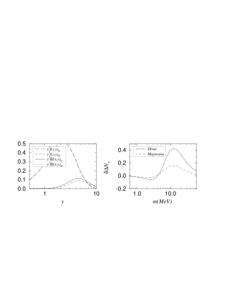
Figure 2: a) The distributions $y^{2}\delta f(x,y)$ for $m_{\nu_{\tau}}=10$ MeV, and $T=1$ MeV ($x=10$) are shown with the corresponding bulk-equilibrium distributions. b) The effect on BBN of the differential heating in units of equivalent $\nu$ degrees of freedom.

4 Results

The mass bounds can be expressed in terms of fit functions of ${{\Delta N}_{\nu}}$. Including all the effects to the electron neutrino distributions discussed above, we find that the Majorana masses are bounded by

$$m^{M}_{\nu} < \sqrt{x}(0.350+0.047\sqrt{x}+0.591x)\;\theta(0.15-x){}$$

$$+ (0.079+0.576x+0.598x^{2}-0.514x^{3}+0.211x^{4})\;\theta(x-0.15){}$$

$$\ m^{M}_{\nu} > 68.59-63.83x+49.18x^{2}-33.09x^{3}+13.18x^{4}-2.17x^{5},$$ (9)

where the units are MeV and I used $x\equiv{{\Delta N}_{\nu}}$. One sees that opening up a window for a stable tau neutrino below the laboratory bound of 23.1 MeV [3] would require relaxing the nucleosynthesis bound to ${{\Delta N}_{\nu}}>1.44$. Then the NS bound of ${{\Delta N}_{\nu}}<1$, together with the above laboratory bound rules out a long-lived Majorana tau neutrino with $m^{M}_{\nu_{\tau}}>0.95$ MeV.

In the Dirac case the upper bound on the disallowed region leads to the constraint

$$m^{D}_{\nu_{\tau}}>41.88-28.47x+20.44x^{2}-13.60x^{3}+5.49x^{4}-0.90x^{5},$$ (10)

where the units are again MeV. The effect of differential heating was for ${{\Delta N}_{\nu}}>1$ to increase the bound from 22 MeV to ${m_{\nu_{\tau}}}>25$ MeV, closing the window below the experimental bound of ${m_{\nu_{\tau}}}<23.1$ MeV at 95% CL.

The computation of the lower bound on the disallowed region is entirely different from that in the preceding cases and completely unchanged by the differential heating effects. I will only quote the results from Fields et al.: for the bound ${{\Delta N}_{\nu}}>1$ they give $m_{\nu_{\mu}}\mbox{\raisebox{-2.58334pt}{~{}$\stackrel{{\scriptstyle<}}{{\sim}}$~{}}}0.31$ MeV and $m_{\nu_{\tau}}\mbox{\raisebox{-2.58334pt}{~{}$\stackrel{{\scriptstyle<}}{{\sim}}$~{}}}0.37$ MeV, with $T_{QCD}=100$ MeV. These constraints are conservative in the sense that they would be somewhat stricter if the QCD transition temperature was chosen higher[1].

In conclusion, even with the weak constraint of ${{\Delta N}_{\nu}}<1$, nucleosynthesis bound is strong enough to exclude a long-lived ($\tau\mbox{\raisebox{-2.58334pt}{~{}$\stackrel{{\scriptstyle>}}{{\sim}}$~{}}}100$ sec) Majorana tau neutrino with ${m_{\nu_{\tau}}}>0.95$ MeV and a Dirac tau neutrino with ${m_{\nu_{\tau}}}>0.37$ MeV.

References

References

- [1] B.D. Fields, K. Kainulainen and K.A. Olive, hep-ph 9512321, CERN-TH/95-335, Astroparticle Physics (in press).
- [2] A.D. Dolgov, S. Pastor and J.W.F. Valle, hep-ph/9602233.
- [3] ALEPH collaboration, Phys. Lett. B 349, 585 (1995); for the update to 23.1 MeV, see A. Gregorio, these proceedings.
- [4] K. Enqvist, K. Kainulainen and V. Semikoz, Nucl. Phys. B 374, 392 (1992).
- [5] K. Enqvist, K. Kainulainen and M. Thomson, Nucl. Phys. B 373, 498 (1992).
- [6] S. Hannestad and J. Madsen, Phys. Rev. Lett. 76, 2848 (1996); erratum hep-ph/9606452.