QCD FROM A LARGE N PERSPECTIVE 

Abstract

The $1/N_{c}$ expansion of QCD can be used to calculate properties of nucleons and $\Delta$ baryons, such as masses, magnetic moments, and pion couplings. The predictions of the $1/N_{c}$ expansion are in excellent agreement with the experimental data. The $1/N_{c}$ expansion also provides an understanding of the relation between the quark model, the Skyrme model, and QCD. This talk reviews some of the recent developments.

1 Introduction

Many features of the baryon sector of QCD have recently been understood both qualitatively and quantitatively using the $1/N_{c}$ expansion.[1]${}^{\!-\,}$[6] Here $N_{c}$ is the number of colors, which is three in the real world. The main results are:

• There is a new symmetry in the baryon sector of QCD in the large $N_{c}$ limit. For two light flavors, the symmetry is a contracted $SU(4)$ symmetry which connects the $u\uparrow$, $u\downarrow$, $d\uparrow$, $d\downarrow$ in a baryon. The $SU(4)_{c}$ symmetry relates the nucleon and $\Delta$, which belong to a single irreducible representation of $SU(4)_{c}$.

• One can compute the higher order $1/N_{c}$ corrections in a systematic way.

• Many results previously obtained in models such as the quark model or the Skyrme model can be proved to be true in QCD to order $1/N_{c}$ or order $1/N_{c}^{2}$. The $1/N_{c}$ expansion explains why some model predictions work better than others; results obtained to order $1/N_{c}^{2}$ work about three times better than those obtained to order $1/N_{c}$. The $1/N_{c}$ expansion provides a unified understanding of different hadronic models, and more importantly, allows one to compute some quantities (e.g. baryon masses, pion couplings, magnetic moments) directly from QCD without any model assumptions.

• The $1/N_{c}$ expansion is intimately connected with baryon chiral perturbation theory. It explains why the $\Delta$ must be included to have a consistent perturbative chiral expansion for baryons. Including the $\Delta$ converts baryon chiral perturbation theory from a strong coupling expansion in powers of $N_{c}$ to a weak coupling expansion in powers of $1/N_{c}$.

• The sigma term puzzle, and the success of various baryon mass formulæ such as the Gell-Mann–Okubo formula can now be understood

• The $1/N_{c}$ expansion provides some information on the nucleon-nucleon potential.[7] (See the talk by D.B. Kaplan in this proceedings.)

2 Large $N_{c}$ Counting Rules

Large $N_{c}$ QCD [8] is a non-trivial theory with confinement and chiral symmetry breaking. The physical states are mesons and baryons. The $1/N_{c}$ counting rules in the meson sector are well-known.[8, 9] The pion decay constant $f_{\pi}$, which is like a one-meson amplitude, is of order $\sqrt{N}_{c}$. Every additional meson in a vertex brings a suppression factor of $1/\sqrt{N}_{c}$. Thus, three-meson amplitudes are of order $1/\sqrt{N}_{c}$, four-meson amplitudes are of order $1/N_{c}$, etc. The counting rules imply that while large $N_{c}$ QCD is a strongly interacting theory in terms of quarks and gluons, it is equivalent to a weakly interacting theory of mesons (and, as we will soon see, baryons). Loop corrections in the meson theory are suppressed by powers of $1/N_{c}$, which is consistent with a semiclassical expansion in powers of $\hbar/N_{c}$.

Large $N_{c}$ baryons are more difficult to study than mesons, because the number of quarks in the baryon is $N_{c}$. The large $N_{c}$ counting rules for baryon amplitudes were given by Witten.[10] The baryon matrix elements of any quark bilinear such as $\bar{\psi}\psi$ are $\leq{\cal O}\left(N_{c}\right)$, because the operator can be inserted on $N_{c}$ possible quark lines. One finds an inequality, rather than an equality, because it is possible that there is a cancellation between the various diagrams. These possible cancellations will turn out to be very important in the analysis that follows. I will assume that the baryon mass $M$ and the axial coupling $g_{A}$ are both of order $N_{c}$, i.e. that there is no cancellation for these two quantities. All models of the baryon, such as the Skyrme model, the non-relativistic quark model, or the bag model, satisfy this assumption. For example, in the non-relativistic quark model $g_{A}=(N_{c}+2)/3$, which gives the well-known value of $5/3$ for $N_{c}=3$.

With these assumptions, the pion-nucleon coupling is of the form

$$(g_{A}/f_{\pi})\ \bar{N}\gamma_{\mu}\gamma_{5}\tau^{a}N\ \partial_{\mu}\pi^{a},$$

and is of order $\sqrt{N}_{c}$, since $g_{A}\sim N_{c}$ and $f_{\pi}\sim\sqrt{N}_{c}$. Recoil effects are of order $1/N_{c}$, and can be neglected. This allows one to simplify the expression for the nucleon axial current. The time component of the axial current between two nucleons at rest vanishes. The space components of the axial current between nucleons at rest can be written as

$$\left\langle N\right|\bar{\psi}\gamma^{i}\gamma_{5}\tau^{a}\psi\left|N\right\rangle=gN_{c}\left\langle N\right|X^{ia}\left|N\right\rangle,$$ (1)

where $\left\langle N\right|X^{ia}\left|N\right\rangle$ and $g$ are of order one. The coupling constant $g$ has been factored out so that the normalization of $X^{ia}$ can be chosen conveniently. $X^{ia}$ is an operator (or $4\times 4$ matrix) defined on nucleon states $p\uparrow$, $p\downarrow$, $n\uparrow$, $n\downarrow$, which has a finite $N_{c}\rightarrow\infty$ limit.

3 Consistency Conditions

One can use the qualitative $1/N_{c}$ counting rules to obtain consistency conditions for various baryonic quantities, such as the axial couplings $X^{ia}$. These consistency conditions can be solved to obtain results for baryons that are in good agreement with the experimental data at $N_{c}=3$.

Consider pion-baryon scattering at fixed energy $E$ (as $N_{c}\rightarrow\infty$) in the chiral limit. The leading contribution is from the pole graphs in Fig. 1, which contribute at order $E$ provided the intermediate state is degenerate with the initial and final states. Otherwise, the pole graph contribution is of order $E^{2}$. In the large $N_{c}$ limit, the pole graphs are of order $N_{c}$. There is also a direct two-pion-$N$ coupling that contributes at order $E$, which is of order $1/N_{c}$ in the large $N_{c}$ limit and can be neglected.

Figure 1: The leading contribution to $\pi N$ scattering to order $E$ in the large $N_{c}$ and chiral limits.

The pion-nucleon scattering amplitude for $\pi^{a}(q)+N(k)\rightarrow\pi^{b}(q^{\prime})+N(k^{\prime})$ from the pole graphs is

$$-i\ q^{i}q^{\prime\,j}{N_{c}^{2}g^{2}\over f_{\pi}^{2}}\left[{1\over q^{0}}X^{jb}X^{ia}-{1\over q^{\prime\,0}}X^{ia}X^{jb}\right],$$ (2)

where the amplitude is written in the form of an operator acting on nucleon states. Both initial and final nucleons are on-shell, so $q^{0}=q^{\prime\,0}$. The product of the $X$’s in Eq. 2 then sums over the possible spins and isospins of the intermediate nucleon. Since $f_{\pi}\sim\sqrt{N}_{c}$, the overall amplitude is of order $N_{c}$, which violates unitarity at fixed energy, and also contradicts the large $N_{c}$ counting rules of Witten. Thus $N_{c}\rightarrow\infty$ QCD with a $I=J=1/2$ nucleon multiplet interacting with a pion is an inconsistent field theory. There must be other states that cancel the order $N_{c}$ amplitude in Eq. 2 so that the total amplitude is order one, consistent with unitarity. One can then generalize $X^{ia}$ to be an operator on this degenerate set of baryon states, with matrix elements equal to the corresponding axial current matrix elements. With this generalization, the form of Eq. 2 is unchanged, and we obtain the first consistency condition for baryons,[1]

$$\left[X^{ia},X^{jb}\right]=0\ .$$ (3)

This consistency condition implies that the baryon axial currents are represented by a set of operators $X^{ia}$ which commute in the $N_{c}\rightarrow\infty$ limit, a result also derived by Gervais and Sakita. [11] There are additional commutation relations,

$$\left[J^{i},X^{jb}\right] = i\,\epsilon_{ijk}\,X^{kb},$$ (4)

$$\left[I^{a},X^{jb}\right] = i\,\epsilon_{abc}\,X^{jc},$$

since $X^{ia}$ has spin one and isospin one.

The algebra in Eqs. 3 and 4 is a contracted SU(4) algebra. To see this, consider the algebra of operators in the non-relativistic quark model, which has an $SU(4)$ symmetry. The operators are

$$J^{i}=q^{\dagger}{\sigma^{i}\over 2}q,\ \ I^{a}=q^{\dagger}{\tau^{a}\over 2}q,\ \ G^{ia}=q^{\dagger}{\sigma^{i}\tau^{a}\over 4}q,$$ (5)

where $J^{i}$ is the spin, $I^{a}$ is the isospin, and $G^{ia}$ are the spin-flavor generators. The commutation relations involving $G^{ia}$ are

$$\left[G^{ia},G^{jb}\right] = \frac{i}{4}\,\epsilon_{ijk}\delta_{ab}\,J^{k}+\frac{i}{4}\,\epsilon_{abc}\delta_{ij}\,I^{c},$$

$$\left[J^{i},G^{jb}\right] = i\,\epsilon_{ijk}\,G^{kb},$$ (6)

$$\left[I^{a},G^{ib}\right] = i\,\epsilon_{abc}\,G^{jc},$$

The algebra for $N_{c}\rightarrow\infty$ baryons in QCD is given by taking the limit

$$X^{ia}\equiv\lim_{N_{c}\rightarrow\infty}{G^{ia}\over N_{c}},$$ (7)

The $SU(4)$ commutation relations Eq. 6 turn into the commutation relations Eqs. 3–4 in the $N_{c}\rightarrow\infty$ limit. The limiting process Eq. 7 is a Lie algebra contraction.

We have just proved that the the $N_{c}\rightarrow\infty$ limit of QCD has a contracted $SU(4)$ symmetry in the baryon sector. The unitary irreducible representations of the contracted Lie algebra can be obtained using the theory of induced representations, and can be shown to be infinite dimensional. The simplest irreducible representation is a tower of states with $I=J=1/2,3/2,etc.$, which is the set of states of the Skyrme model, or the large $N_{c}$ non-relativistic quark model. More complicated irreducible representations correspond to baryons containing strange quarks.

The pion-baryon coupling matrix $X^{ia}$ can be completely determined (up to an overall normalization $g$), since it is a generator of the $SU(4)_{c}$ algebra. It is easy to show that the $N_{c}\rightarrow\infty$ QCD predictions for the pion-baryon coupling ratios are the same as those obtained in the Skyrme model or non-relativistic quark model[12]${}^{\!-\,}$[14] in the $N_{c}\rightarrow\infty$ limit, because both these models also have a contracted $SU(4)$ symmetry in this limit. In the Skyrme model, the axial current in the $N_{c}\rightarrow\infty$ limit is $X^{ia}\propto{\rm Tr}A\tau^{i}A^{-1}\tau^{a}$. The $X$’s commute (and so form part of an $SU(4)_{c}$ algebra), since $A$ is a $c$-number. We have already seen how the quark model algebra reduces to $SU(4)_{c}$ in the large $N_{c}$ limit.

4 $1/N_{c}$ Corrections

What makes the $1/N_{c}$ expansion for baryons interesting is that it is possible to compute the $1/N_{c}$ corrections. This allows one to compute results for the physical case $N_{c}=3$, rather than for the strict $N_{c}=\infty$ limit, which is only of formal interest.

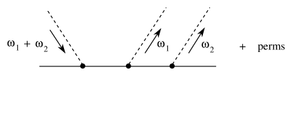
Figure 2: The leading contribution to $\pi N\rightarrow\pi\pi N$ in the large $N_{c}$ and chiral limits.

The $1/N_{c}$ corrections to the axial couplings $X^{ia}$ are determined by considering the scattering process $\pi^{a}+N\rightarrow\pi^{b}+\pi^{c}+N$ at low energies. The baryon pole graphs that contribute in the $N_{c}\rightarrow\infty$ limit are shown in Fig. 2. The axial coupling $X^{ia}$ can be expanded in a series in $1/N_{c}$,

$$X^{ia}=X^{ia}_{0}+{1\over N_{c}}X^{ia}_{1}+\ldots$$ (8)

The amplitude for pion-nucleon scattering from the diagrams in Fig. 2 is proportional to

$$N_{c}^{3/2}\left[X^{ia},\left[X^{jb},X^{kc}\right]\right],$$

and violates unitarity unless the double commutator vanishes at least as fast as $N_{c}^{-3/2}$, so that the amplitude is at most of order one. (In fact, one expects that the double commutator is of order $1/N_{c}^{2}$ since the corrections should only involve integer powers of $1/N_{c}$. This result also follows from the $N_{c}\rightarrow\infty$ counting rules which imply that each additional pion gives a factor of $1/\sqrt{N_{c}}$ in the amplitude.) Substituting Eq. 8 into the constraint gives the consistency condition

$$\left[X^{ia}_{0},\left[X_{1}^{jb},X^{kc}_{0}\right]\right]+\left[X^{ia}_{0},\left[X^{jb}_{0},X_{1}^{kc}\right]\right]=0,$$ (9)

using $\left[X^{ia}_{0},X^{jb}_{0}\right]=0$ from Eq. 3. The only solution to Eq. 9 is that $X_{1}^{ia}$ is proportional to $X_{0}^{ia}$.[1] This can be verified by an explicit computation of $X_{1}^{ia}$ using reduced matrix elements, or by using group theoretic methods.[3, 6] Thus we find that

$$X^{ia}=\left(1+{c\over N_{c}}\right)X_{0}^{ia}+{\cal O}\left({1\over N_{c}^{2}}\right),$$ (10)

where $c$ is an unknown constant. The first correction to $X^{ia}$ is proportional to the lowest order value $X_{0}^{ia}$, so the $1/N_{c}$ correction to the axial coupling constant ratios vanishes.[1] We have now shown that the predictions for the ratios of pion couplings, such as $g_{\pi NN}/g_{\pi N\Delta}$ or $g_{\pi NN}/g_{\pi\Delta\Delta}$ are equal to the prediction in the Skyrme model up to corrections of order $1/N_{c}^{2}$. The Skyrme model results for the ratios of couplings are known to agree with experiment to about 10% accuracy.[15]

At order $1/N_{c}$, the baryons in an irreducible representation of the contracted $SU(4)$ Lie algebra are no longer degenerate, but are split by an order $1/N_{c}$ mass term $\Delta M$. The intermediate baryon propagator in Eq. 2 should be replaced by $1/(E-\Delta M)$. The energy $E$ of the pion is order one, whereas $\Delta M$ is of order $1/N_{c}$, so the propagator can be expanded to order $1/N_{c}$ as

$${1\over E-\Delta M}={1\over E}+{\Delta M\over E^{2}}+\ldots\ \ .$$ (11)

Including the $1/N_{c}$ corrections to the propagator does not affect the derivation of Eq. 3, as the two terms in Eq. 11 have different energy dependences. The first term leads to the consistency condition Eq. 3 and the second gives the consistency condition on the baryon masses,[2, 3]

$$\left[X^{ia},\left[X^{jb},\left[X^{kc},\Delta M\right]\right]\right]=0.$$ (12)

This constraint can be used to obtain the $1/N_{c}$ corrections to the baryon masses. The constraint Eq. 12 is equivalent to a simpler constraint obtained by Jenkins using chiral perturbation theory[2]

$$\left[X^{ia},\left[X^{ia},\Delta M\right]\right]={\rm constant}.$$ (13)

The solution of Eq. 12 or 13 is that the baryon mass splitting $\Delta M$ must be proportional to $J^{2}/N_{c}=j(j+1)/N_{c}$, where $j$ is the spin of the baryon.[2] This is precisely the form of the baryon mass splitting in the Skyrme model.

The structure of the $1/N_{c}$ corrections shows that the expansion parameter is $J/N_{c}$, where $J$ is the spin of the baryon. For example, the baryon mass spectrum including the $J^{2}/N_{c}$ mass splitting has the form shown in Fig. 3. The correction terms are only small near the bottom of the (infinite) baryon tower. For this reason, the $1/N_{c}$ expansion will only be considered for baryons with spin $J$ held fixed as $N_{c}\rightarrow\infty$.

Figure 3: The baryon mass spectrum including the $J^{2}/N_{c}$ term.

5 Results

It is relatively simple to obtain consistency conditions such as Eq. 3,9 or 12 using the $1/N_{c}$ expansion. Solving these equations is straightforward, but will not be described here. The general solution for any physical quantity ${\cal M}$ has the form of a series expansion,

$${\cal M}=N_{c}^{r}\ {\cal P}\left(X^{ia},{J^{k}\over N_{c}},{I^{a}\over N_{c}}\right),$$ (14)

where ${\cal P}$ is a polynomial in its arguments, with each operator appearing with a coefficient $c\left(1/N_{c}\right)$ which is order one as $N_{c}\rightarrow\infty$. The overall power of $r$ is given by the $N_{c}$ power counting rule for the quantity ${\cal M}$ being considered. All the terms in the polynomial ${\cal P}$ must have the same spin and isospin as ${\cal M}$. In addition, there are a set of operator identities that allow one to eliminate many terms in ${\cal P}$ with contracted spin or isospin indices. For two flavors, these identites are [3]

$$X^{ia}X^{ib}=\delta^{ab}, X^{ia}X^{ja}=\delta^{ij},$$

$$X^{ia}J^{i}=-I^{a}, X^{ia}I^{a}=-J^{i},$$ (15)

$$\epsilon_{ijk}X^{ia}X^{jb}=\epsilon_{abc}X^{kc}, \epsilon_{abc}X^{ia}X^{jb}=\epsilon_{ijk}X^{kc}.$$

For example, if ${\cal M}$ is the baryon mass, $r=1$ since the baryon mass is of order $N_{c}$. The general expansion has the form

$$M=N_{c}\left(c_{0}+c_{1}{J^{2}\over N_{c}^{2}}+c_{2}{J^{4}\over N_{c}^{4}}+\ldots\right).$$ (16)

All other terms in ${\cal P}$ can be eliminated using Eq. 15. At present, it is not known how to compute the coefficients $c_{i}$.

One can obtain relations among baryon quantities by working to a given order in $1/N_{c}$, neglecting all higher order terms in ${\cal P}$. The accuracy of the relations is determined by the order in $1/N_{c}$ of the neglected operators. As a trivial example, consider the baryon masses in the two flavor case. The physical states are the $N$ and $\Delta$, with $I=J=1/2$ and $3/2$, respectively. To lowest order, one finds that

$$M_{N}=N_{c}c_{0}+{\cal O}\left(1/N_{c}\right),\ \ \ M_{\Delta}=N_{c}c_{0}+{\cal O}\left(1/N_{c}\right),$$ (17)

and the prediction

$$M_{N}=M_{\Delta}+{\cal O}\left(1/N_{c}\right).$$ (18)

This relation is a homogenous relation among the baryon masses. It is convenient to write Eq. 18 in the form

$${M_{\Delta}-M_{N}\over\left(M_{\Delta}+M_{N}\right)/2}={\cal O}\left(1/N_{c}^{2}\right),$$ (19)

where the numerator is the difference of the two sides of Eq. 18, and the denominator is the average of the two sides. The form Eq. 19 does not depend on the overall scale of Eq. 18. Including the first correction gives

$$M_{N}=N_{c}c_{0}+c_{1}{3\over 4N_{c}}+{\cal O}\left(1/N_{c}^{3}\right),\ M_{\Delta}=N_{c}c_{0}+c_{1}{15\over 4N_{c}}+{\cal O}\left(1/N_{c}^{3}\right)$$ (20)

In this simple example, there is no relation including the $1/N_{c}$ correction because two masses are given in terms of two parameters. However, one obtains many non-trivial predictions when the results are extended to three flavors.

The baryon masses have been analyzed in a simultaneous expansion in $SU(3)$ breaking (due to $m_{s}$), isospin breaking, and $1/N_{c}$ by Jenkins and Lebed.[16] They obtain a number of relations of the form Eq. 19. Their relations for isospin averaged masses (such as $(M_{P}+M_{N})/2$) are shown graphically in Fig. 4. What is plotted are mass splittings of the form Eq. 19; the error bars are the experimental errors on the measured baryon masses. The relations are valid to some order in $\epsilon$ and $1/N_{c}$, where $\epsilon\sim 0.3$ is a measure of $SU(3)$ breaking. It is clear from Fig. 4 that the $1/N_{c}$ expansion explains the hierarchy of the baryon mass relations. For example, there are three relations which should be true up to corrections of order $\epsilon$. One of them is order $\epsilon/N_{c}$, one of order $\epsilon/N_{c}^{2}$ and one of order $\epsilon/N_{c}^{3}$. The hierarchy between these relations is obvious from Fig. 4. An $SU(3)$ analysis alone does not explain why some of the order $\epsilon$ relations work better than others. Similarly, the $1/N_{c}$ expansion explains the hierarchy in the two $\epsilon^{2}$ relations. One can also see that the $1/N_{c}^{2}$ mass relation, which is not suppressed by $SU(3)$ breaking, works to about 11%. One can understand the baryon mass spectrum to a fractional error of 0.001 (i.e. $\sim 1$ MeV) in the isospin averaged masses using $1/N_{c}$ and $SU(3)$ symmetry.

Figure 4: Plot of the isospin averaged mass relations of Jenkins and Lebed.[16]. The error bars are the experimental errors on the measured baryon masses. In terms of the $SU(3)$ breaking parameter $\epsilon\sim 0.3$, and $1/N_{c}$, the open circle is a relation of order $1/N_{c}^{2}$, the three solid triangles are relations of order $\epsilon/N_{c}$, $\epsilon/N_{c}^{2}$, and $\epsilon/N_{c}^{3}$, the open squares are relations of order $\epsilon^{2}/N_{c}^{2}$, and $\epsilon^{2}/N_{c}^{3}$ and the $\times$ is a relation of order $\epsilon^{3}/N_{c}^{3}$. The $1/N_{c}$ hierarchy is obvious.

A similar analysis can be done for the baryon magnetic moments.[17, 18] The $1/N_{c}$ relations for the isovector and isoscalar magnetic moments are shown in Fig. 5. Most of the magnetic moment relations derived using the quark model can now be obtained directly from QCD, to some order in $1/N_{c}$. The $1/N_{c}$ expansion also explains why some relations work better than others; something which is left unexplained by the quark model. There is also one new relation. Relation 7, which relates the $\Delta^{+}\rightarrow p$ transition moment to $p-n$, is a $1/N_{c}^{2}$ relation (which is also true in the quark model) which works to 30%. This is one instance in which the $1/N_{c}^{2}$ correction is substantial. All the $1/N_{c}$ relations are homogeneous, and do not set the scale of the magnetic moments. In the quark model, one can get a good estimate of the size of the magnetic moments from the constituent quark mass. This is not explained by the $1/N_{c}$ expansion.

Figure 5: Plot of the magnetic moment relations. The error bars are the experimental errors on the measured magnetic moments. The open points are relations which are true in $1/N_{c}$ and in the non-relativistic quark model, the filled point is a relation which is true in $1/N_{c}$, but has no quark model analog. The circles are relations of order $1/N_{c}$, the squares of order $1/N_{c}^{2}$, and the triangles of order $\epsilon/N_{c}$.

6 Other Results

There are many other results that have been obtained using the $1/N_{c}$ expansion, some of which are summarized here.

• One loop corrections to the baryon axial currents are large, and disagree with experiment, unless one includes intermediate $\Delta$ states in loops.[19] There are large cancellations between $N$ and $\Delta$ intermediate states. The best fit values for the axial couplings when $\Delta$’s are included are close to $SU(6)$ values.[19] The $1/N_{c}$ explains all of these results. One can show that the one-loop corrections to the axial currents have the structure

  $$N_{c}\left[X,\left[X,X\right]\right]$$ (21)

  Eq. 21 is a commutator that is constrained by the large $N_{c}$ consistency conditions, and is of order $1/N_{c}^{2}$. Thus including intermediate $\Delta$ states produces a cancellation to two orders in $1/N_{c}$, so the one-loop correction is of order $1/N_{c}$. This cancellation converts an expansion in $N_{c}$ to a semiclassical expansion in $\hbar/N_{c}$. If intermediate $\Delta$ states are not included, the one-loop correction is of order $N_{c}$ times the tree level result, since the cancellation conditions on $X$ do not hold in the nucleon sector alone. Baryon chiral perturbation theory without a $\Delta$ is a strong coupling expansion in powers of $N_{c}$. The strongly coupled theory presumably dynamically generates a $\Delta$.

• One loop corrections to the baryon masses are large ($\sim$ 500 MeV). Most of the correction is $SU(3)$ singlet or octet, so the large non-linearities do not violate the Gell-Mann–Okubo formula.[20] This resolves the sigma-term puzzle.[21]

• Certain Skyrme model results on baryons containing heavy quarks using the bound state approach to strangeness of Callan and Klebanov follow from large $N_{c}$ alone.[2, 22, 23]

• The chiral bag model arises naturally in the $N_{c}\rightarrow\infty$ limit.[24, 25]

• One can compute the $F/D$ ratio and an equal spacing rule for the axial couplings in $\beta$ decay.[3]

• One understands the $s$-wave hyperon non-leptonic decay amplitudes.[26, 6]

• One can analyze $SU(3)$ breaking in the baryon axial vector currents.[27] One finds that $\Delta u+\Delta d-2\Delta s$ is shifted from its $SU(3)$ symmetric value of $0.6$ to $0.3\pm 0.1$. This affects the interpretation of the recent experiments on the $g_{1}$ structure function of the nucleon.

7 Conclusions

The $1/N_{c}$ expansion shows that most of the spin-flavor structure of baryons can be understood using contracted $SU(4)$ symmetry. It provides a unifying symmetry which connects the various quark models (non-relativistic, bag), the Skyrme model, and QCD. The $1/N_{c}$ expansion explains many results found earlier in baryon chiral perturbation theory in a systematic way, and it is possible to combine baryon chiral perturbation theory with the $1/N_{c}$ expansion of QCD.[28]

References

References

- [1] R. Dashen and A.V. Manohar, Phys. Lett. B 315, 425 (1993), Phys. Lett. B 315, 438 (1993).
- [2] E. Jenkins, Phys. Lett. B 315, 431 (1993), Phys. Lett. B 315, 441 (1993), Phys. Lett. B 315, 447 (1993).
- [3] R. Dashen, E. Jenkins, and A.V. Manohar, Phys. Rev. D 49, 4713 (1994).
- [4] C. Carone, H. Georgi, and S. Osofsky, Phys. Lett. B 322, 227 (1994).
- [5] M. Luty and J. March-Russell, Nucl. Phys. B 426, 71 (1994).
- [6] R. Dashen, E. Jenkins, and A.V. Manohar, Phys. Rev. D 51, 3697 (1995).
- [7] D.B. Kaplan and A.V. Manohar (unpublished).
- [8] G. ’t Hooft, Nucl. Phys. B 72, 461 (1974).
- [9] S. Coleman, in Aspects of Symmetry (Cambridge University Press, Cambridge, 1989).
- [10] E. Witten, Nucl. Phys. B 160, 57 (1979).
- [11] J.-L. Gervais and B. Sakita, Phys. Rev. D 30, 1795 (1984).
- [12] A.V. Manohar, Nucl. Phys. B 248, 19 (1984).
- [13] G. Karl and J.E. Paton, Phys. Rev. D 30, 238 (1984).
- [14] M. Cvetic, and J. Trampetic, Phys. Rev. D 33, 1437 (1986).
- [15] G.S Adkins, C.R. Nappi, and E. Witten, Nucl. Phys. B 228, 552 (1983).
- [16] E. Jenkins and R.F. Lebed, Phys. Rev. D 52, 282 (1995).
- [17] E. Jenkins and A.V. Manohar, Phys. Lett. B 335, 452 (1994).
- [18] M. Luty, J. March-Russell, and M. White, Phys. Rev. D 51, 2332 (1995).
- [19] E. Jenkins and A.V. Manohar, Phys. Lett. B 255, 558 (1991), Phys. Lett. B 259, 353 (1991).
- [20] E. Jenkins, Nucl. Phys. B 368, 190 (1992), E. Jenkins and A.V. Manohar, Phys. Lett. B 281, 336 (1992).
- [21] R.L. Jaffe, Phys. Rev. D 21, 3215 (1980).
- [22] C. Callan and I. Klebanov, Nucl. Phys. B 262, 365 (1985), C. Callan, K. Hornbostel, and I. Klebanov, Phys. Lett. B 202, 269 (1988).
- [23] E. Jenkins, A.V. Manohar, and M.B. Wise, Nucl. Phys. B 396, 27 (1993), Nucl. Phys. B 396, 38 (1993), E. Jenkins and A.V. Manohar, Phys. Lett. B 294, 273 (1992), Z. Guralnik, M.E. Luke, A.V. Manohar, Nucl. Phys. B 390, 474 (1993).
- [24] N. Dorey, J. Hughes, and M. Mattis, Phys. Rev. Lett. 73, 1211 (1994).
- [25] A.V. Manohar, Phys. Lett. B 336, 502 (1994).
- [26] E. Jenkins, Nucl. Phys. B 375, 561 (1992).
- [27] J. Dai, R.F. Dashen, E. Jenkins, and A.V. Manohar, Phys. Rev. D 53, 273 (1996).
- [28] E. Jenkins, Phys. Rev. D 53, 2625 (1996).