Abstract:
Recent measurements of the electron and muon neutrino masses squared are interpreted as an indication that neutrinos are faster than light particles – tachyons. The tritium beta decay amplitude is calculated for the case of the tachyonic electron neutrino. Agreement of the theoretical prediction with the shape of the recently measured electron spectra is discussed. Amplitude for the three body decay of the tachyonic neutrino, $\nu_{i}\rightarrow\nu_{i}\nu_{j}\overline{\nu}_{j}$, is calculated. It is shown that this decay may explain the solar neutrino problem without assuming neutrino oscillations. Predictions for short and long baseline experiments are commented. Future experimental activities are suggested.

1 Introduction

In all recent measurements the values of the mass squared obtained for the electron [1, 2, 3, 4, 5, 6, 7, 8] and muon [9, 10] neutrinos are negative, as summarised in table 1. This observation requires an explanation which should be searched for on the grounds of both conventional as well as nonstandard concepts.

At present the best method of determining the mass of the electron neutrino is to fit an appropriate theoretical formula in the endpoint region of the electron energy spectrum measured in the $\beta$ decay of tritium (electron kinetic energy at endpoint amounts to $\approx 18570\;{\rm eV}$).

Flavour		$m^{2}$			Year	Ref.
	$-22$	$\pm$	$17\pm 14\;$	${\rm eV}^{2}$	1996	[1]
	$-20.6$	$\pm$	$5.8\;$	${\rm eV}^{2}$	1996	[2]
	$-130$	$\pm$	$20\pm 15\;$	${\rm eV}^{2}$	1995	[3]
$\nu_{e}$	$-22$	$\pm$	$4.8\;$	${\rm eV}^{2}$	1995	[4]
	$-39$	$\pm$	$34\pm 15\;$	${\rm eV}^{2}$	1993	[5]
	$-24$	$\pm$	$48\pm 61\;$	${\rm eV}^{2}$	1992	[6]
	$-65$	$\pm$	$85\pm 65\;$	${\rm eV}^{2}$	1991	[7]
	$-147$	$\pm$	$68\pm 41\;$	${\rm eV}^{2}$	1991	[8]
$\nu_{\mu}$	$-0.143$	$\pm$	$0.024\;$	${\rm MeV}^{2}$	1996	[9]
	$-0.016$	$\pm$	$0.023\;$	${\rm MeV}^{2}$

Table 1: Recent results of the electron and muon neutrino mass squared measurements. The first uncertainty is statistical, the second systematic.

Improving resolution of spectrometers used in certain recent experiments lead to an observation of two unexpected details in the electron energy spectrum, presently often referred to as anomalies.

One anomaly appears as an enhancement located close to the endpoint in the integral electron energy spectrum [2, 3, 4], as shown in figs. 1 and  2. Branching ratio of this structure comes out to be of the order of $3\cdot 10^{-9}$ [3] or $10^{-10}$ [4]. Presently an effort is spent to understand the effect on the grounds of atomic physics [11] and statistics [12].

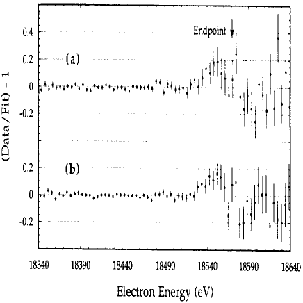
Figure 1: Ratio of measured and fitted spectra (Kurie plot) from the LLNL experiment [3].

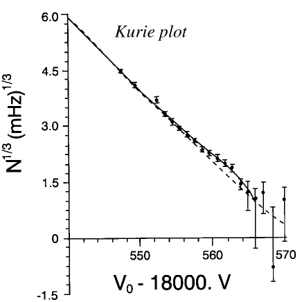
Figure 2: Integral electron energy spectrum in tritium decay (Kurie plot) measured in the Troitsk experiment [4].

The second anomaly, located at lower energies, is related to the slope of the measured electron energy spectrum. If the theoretical spectrum is fitted in the energy range below approximately $18300\;{\rm eV}$ then the endpoint occurs at a lower value of energy. This anomaly was interpreted as a manifestation of a missing spectral component with about $4\%$ branching ratio and the endpoint energy around $18400\;{\rm eV}$ [4] or $18500\;{\rm eV}$ [5].

The mass squared of the muon neutrino has been determined from the measured muon momentum in the $\pi^{+}$ decay at rest. The latest, most precise results also indicate a negative value [9]. The two entries in table 1 correspond to different values of the charged pion mass [10]. This ambiguity soon should be resolved by additional measurements [9].

Until now there have been no experiments dedicated to determine the tau neutrino mass. The latest analysis [13] lead to a result with large uncertainties and as such cannot be considered in the context of the idea presented in this paper.

In view of the above results for the neutrino masses squared we elaborate on the hypothesis that neutrinos are tachyons. The aim of this paper is to present a confrontation of experimental data with theoretical calculations performed for processes involving tachyonic neutrinos. It will be shown that the measured shape of the electron spectrum near the endpoint in the tritium decay is qualitatively consistent with that predicted from the decay involving the tachyonic electron neutrino. The amplitude for the three body lepton flavour conserving decay of the tachyonic neutrino, $\nu_{i}\rightarrow\nu_{i}\nu_{j}\overline{\nu}_{j}$, is calculated and predictions for certain phenomena discussed.

In the following sections various values of tachyonic neutrino masses appear as a result of certain assumptions. Tachyons, like massive and massless particles, are subject to gravitational interactions too. However at the present, early stage of our work we have not yet grounds to comment possible constraints on tachyonic neutrino masses resulting from considerations on the cosmological scale.

2 Theoretical considerations

It has been a common conviction that tachyons could not exist for several reasons related to fact that they are moving with superluminal velocities: negative energies, causality violation, vacuum instability and others. Despite a significant theoretical effort no solution of these problems has been found within the framework of the Einstein–Poincaré (EP) relativity. However the recently proposed causal theory of tachyons [14, 15, 16] is free of these difficulties.

The main idea is based on two well known facts: $(i)$ the definition of a coordinate time depends on the synchronisation scheme; $(ii)$ synchronisation scheme is a convention, because no experimental procedure exists which makes it possible to determine the one-way velocity of light without use of superluminal signals. Therefore there is a freedom in the definition of the coordinate time. The standard choice is the Einstein–Poincaré (EP) synchronisation with one-way light velocity isotropic and constant. This choice leads to the extremely simple form of the Lorentz group transformations but the EP coordinate time implies a covariant causality for time-like and light-like trajectories only. We choose a different synchronisation, namely that of Chang–Tangherlini (CT) preserving invariance of the notion of the instant-time hyperplane [17, 18]. In this synchronisation scheme the causality notion is universal and space-like trajectories are physically admissible too. The price is the more complicated form of the Lorentz transformations incorporating transformation rules for velocity of distinguished reference frame (preferred frame). The EP and CT descriptions are entirely equivalent if we restrict ourselves to time-like and light-like trajectories; however a consistent description of tachyons is possible only in the CT scheme. A very important consequence is that if tachyons exist then the relativity principle is broken, i.e. there exists a preferred frame of reference, however the Lorentz symmetry is preserved. As we know, in the real world we have such a locally distinguished frame – namely the cosmic background radiation frame.

The interrelation between EP ($x_{E}$) and CT ($x$)coordinates reads:

$$x_{E}^{0}=x^{0}+u^{0}\vec{u}\vec{x}\quad,\qquad\vec{x}_{E}=\vec{x}$$ (1)

where $u^{\mu}$ is the four-velocity of the privileged frame as seen from the frame ($x^{\mu}$).

In refs. [14, 15, 16] a fully consistent, Poincaré covariant quantum field theory of tachyons was given. In particular, the elementary tachyonic states are labelled by helicity. In the case of the fermionic tachyon with helicity $-\frac{1}{2}$ the corresponding field equation reads:

$$\left(\gamma^{5}\left(i\gamma\partial\right)-\kappa\right)\psi=0$$ (2)

where the bispinor field $\psi$ is simultaneously an eigenvector of the helicity operator with eigenvalue $\frac{1}{2}$. Here the $\gamma$-matrices are expressed by the standard ones in analogy to the relation (1). The solution of (2) is given by:

$$\psi(x,u)\\ =\frac{1}{(2\pi)^{\frac{3}{2}}}\int d^{4}k\,\delta(k^{2}+\kappa^{2})\theta(k^{0})\left[w(k,u)e^{ikx}b^{\dagger}(k)+v(k,u)e^{-ikx}a(k)\right]$$ (3)

where the operators $a$ and $b$ correspond to neutrino and antineutrino, respectively. The amplitudes $v$ and $w$ satisfy the following conditions:

$$w(k,u)\bar{w}(k,u)=(\kappa-\gamma^{5}k\gamma)\frac{1}{2}\left(1-\frac{\gamma^{5}[k\gamma,u\gamma]}{2\sqrt{q^{2}+\kappa^{2}}}\right)$$ (4)

$$v(k,u)\bar{v}(k,u)=-(\kappa+\gamma^{5}k\gamma)\frac{1}{2}\left(1-\frac{\gamma^{5}[k\gamma,u\gamma]}{2\sqrt{q^{2}+\kappa^{2}}}\right)$$ (5)

$$\bar{w}(k,u)\gamma^{5}u\gamma w(k,u)=\bar{v}(k,u)\gamma^{5}u\gamma v(k,u)=2q$$ (6)

$$\bar{w}(k^{\Pi},u)\gamma^{5}u\gamma v(k,u)=0.$$ (7)

Here $q=u_{\mu}k^{\mu}$ is equal to the energy of the tachyon in the preferred frame and $\Pi$ denotes the space inversion operation. It is easy to check that in the massless limit $\kappa\rightarrow 0$ the above relations give the Weyl’s theory.

3 Tritium $\beta$ decay with the tachyonic neutrino

Until now the mass squared of the electron neutrino has been determined by fitting the measured integral electron energy spectrum with a function comprising an expression for the decay probability. The integral form of this expression is as follows (neglecting summation over final states) [5]:

$$S(E)\sim p_{e}(E_{e}+m_{e})(E_{0}-E_{e})\sqrt{(E_{0}-E_{e})^{2}-m_{\nu_{e}}^{2}}$$ (8)

where $E_{e},\;p_{e},\;m_{e}$ are the electron kinetic energy, momentum and mass, $E_{0}$ is the endpoint kinetic energy and $m_{\nu_{e}}^{2}$ is the square of the electron antineutrino mass. This formula is obtained from the standard calculation of the three body weak decay, including a massive neutrino. However if one wants to test the hypothesis that neutrinos are tachyons, this formula is no longer valid for that purpose even if the sign in front of the $m_{\nu_{e}}^{2}$ term is changed. The correct expression can be obtained from a similar, although by far more complicated, calculation.

Let us consider the $\beta$ decay in the framework of section 2, using effective four-fermion interaction. In the first order of the perturbation series the decay rate for the process: $n\longrightarrow p^{+}+e^{-}+\overline{\nu}_{e}$ with the tachyonic electron antineutrino reads:

$$d\Gamma=\frac{1}{4m_{n}(2\pi)^{5}}d\Phi_{3}\left|M\right|^{2},$$ (9)

where $d\Phi_{3}$ is the phase-space volume element:

$$d\Phi_{3}=\,\theta(k^{0})\,\theta(l^{0})\,\theta(r^{0})$$ ⋅ (10)

$$\delta(k^{2}-m_{p}^{2})\,\delta(l^{2}-m_{e}^{2})\,\delta(r^{2}+\kappa^{2})\,\delta^{4}(p-k-l-r)\,d^{4}k\,d^{4}l\,d^{4}r$$

while

$$\left|M\right|^{2}=2\,G_{F}^{2}\,{\rm Tr}\left[u_{e}\overline{u}_{e}\gamma^{\mu}w\overline{w}\gamma^{\nu}\right]\\ {\rm Tr}\left[u_{p}\overline{u}_{p}\gamma_{\mu}\left(1-g_{A}\gamma^{5}\right)u_{n}\overline{u}_{n}\gamma_{\nu}\left(1-g_{A}\gamma^{5}\right)\right].$$ (11)

Here $p,k,l,r$ are the four-momenta of $n,p^{+},e^{-}$ and $\overline{\nu}$ respectively; the corresponding masses are denoted by $m_{n},m_{p},m_{e}$ and $\kappa$ (in the case of tritium decay $m_{n}$ and $\;m_{p}$ denote the masses of ${}^{3}H$ and ${}^{3}He$). $G_{F}$ and $g_{A}$ are the Fermi constant and the axial coupling constant. The amplitudes $u_{n},\overline{u}_{n},u_{p},\overline{u}_{p},u_{e},\overline{u}_{e}$ satisfy usual polarisation relations: $u_{n}\overline{u}_{n}=p\gamma+m_{n}$, $u_{p}\overline{u}_{p}=k\gamma+m_{p}$, $u_{e}\overline{u}_{e}=l\gamma+m_{e}$ whereas $w\overline{w}$ is given by eq. 4. After elementary calculations eq. 11 reads:

$$\left|M\right|^{2}=16\,G_{F}^{2}\left\{\left[m_{n}m_{p}(1-g_{A}^{2})-(kp)(1+g_{A}^{2})\right]\right.\cdot$$ (12)

$$\cdot\left(4m_{e}\kappa-\frac{1}{\sqrt{(ur)^{2}+\kappa^{2}}}\left[4\left(\kappa^{2}(lu)+(lr)(ur)\right)-2\kappa^{2}(lu)-2(ur)(lr)\right]\right)+\mbox{}$$

$$\mbox{}+(1+g_{A}^{2})\left(2m_{e}\kappa(pk)-\frac{1}{\sqrt{(ur)^{2}+\kappa^{2}}}\right.\cdot$$

$$\mbox{\quad}\cdot\left[2(pk)\left(\kappa^{2}(lu)+(lr)(ur)\right)-2\kappa^{2}\left((pl)(uk)+(kl)(up)\right)\right.+\mbox{}$$

$$\mbox{}\qquad-\left.\left.2(ur)\left((pl)(kr)+(kl)(pr)\right)\right]\right)+\mbox{}$$

$$\mbox{}+4g_{A}\left.\left[(pr)(kl)-(pl)(kr)+\frac{m_{e}\kappa}{\sqrt{(ur)^{2}+\kappa^{2}}}\left((kr)(up)-(pr)(uk)\right)\right]\right\}$$

Because the Solar System is almost at rest relatively to the cosmic background radiation frame we can calculate the electron energy spectrum $d\Gamma/dl^{0}$ in this frame with sufficient precision. The resulting formula is rather complicated (16); we present it in the Appendix.

Formula (9) gives identical results in the limit $\kappa^{2}\rightarrow 0$ as that for the massless neutrino. Differential electron energy spectra near the endpoint for massless and tachyonic neutrinos are shown in fig. 3a (we used the following values for the masses of ${}^{3}{\rm H}$ and ${}^{3}{\rm He}$: $2809.94\;{\rm MeV}$ and $2809.41\;{\rm MeV}$). The distinctive feature of the spectrum near the endpoint in the tachyonic case is the enhancement with a step-like termination. Function (16) goes to zero over a narrow range of energy, contrary to a monotonic character in the cases of the massless (and massive) neutrino. In order to allow for a qualitative comparison with the measurement of ref. [4], the electron spectrum given by (16) was integrated and smeared with constant experimental energy resolution of $4\;{\rm eV}$ (assumed Gaussian).

Figure 3: (a) Theoretical differential energy spectrum $d\Gamma/dE$ for tritium decay with the tachyonic electron antineutrino of mass $\kappa$; (b) smeared integral spectrum (Kurie plot) – endpoint energy indicated by arrow. Curves drawn for masses: $\kappa=0,10,20\;{\rm eV}$.

As a result the step-like endpoint structure of the differential spectrum appeared as an enhancement in the integral electron energy distribution, as shown in fig. 3b. Position, magnitude and width of the enhancement depend on the tachyonic electron neutrino mass, $\kappa$. At this stage of investigations we may conclude that using formula (16) it is possible to reproduce qualitatively the enhancement in the electron energy spectrum near the endpoint if a sufficiently large value of the tachyonic neutrino mass is taken. Indeed, no ‘bump’ is seen for $\kappa=10\;{\rm eV}$ while it is already clearly marked for $\kappa=20\;{\rm eV}$. It is indispensable to perform a fit to the experimental spectrum; however we were not in possession neither of the data nor the details of the apparatus.

For the purpose of considerations presented in section 4 we need an input value for the tachyonic electron antineutrino mass. The value $\kappa\approx 5\;{\rm eV}$, quoted in refs. [2, 4], is not meaningful for the tachyonic hypothesis since it was obtained by fitting function (8) which describes the massive neutrino ($m^{2}>0$). As an ‘educated guess’ (fig. 3b) we take $20\;{\rm eV}$ for the mass of the tachyonic electron neutrino.

4 Decays of tachyonic neutrinos

4.1 Introduction

Tachyonic neutrinos are in general unstable. Similarly to a three body decay of a massive particle, a tachyon may decay into three tachyons. In the latter case however a specific channel is allowed with the initial tachyon appearing also in the final state. In the case of tachyonic neutrinos the corresponding process would be the decay of a neutrino of flavour ‘$i$’ into itself and a neutrino – antineutrino pair of flavour ‘$j$’: $\nu_{i}\rightarrow\nu_{i}\nu_{j}\overline{\nu}_{j}$, where $i,j=e,\mu,\tau$, as shown in fig. 4.

                          

Figure 4: Lepton flavour conserving decays of the tachyonic neutrino.

Another important mode is the radiative decay, $\nu_{i}\rightarrow\nu_{i}\gamma$, shown in the same figure. In both processes the lepton family number is conserved, contrary to those involving a massive neutrino. In this section we deal with the three body decay and calculate partial widths $\Gamma_{ij}$ in order to find out whether the tachyonic hypothesis is not in contradiction with established observations.

Tachyonic neutrino decays mean an additional, qualitatively similar process to oscillations. Consider a beam of neutrinos of a given flavour, characterised by a certain energy spectrum. As a result of decays new flavours appear as a function of distance (including antineutrinos in neutrino beams and vice versa) but in a pattern much more complicated than in the case of oscillations. ¿From the theoretical point of view the decay has a clear advantage over the latter since its magnitude can be calculated within the theory of weak interactions; masses of tachyonic neutrinos, which can be determined from independent measurements, are the only input parameters in that case.

4.2 Derivation of formulae

Assuming universality of weak interactions we can calculate the decay rate for the process $\nu_{i}\rightarrow\nu_{i}\nu_{j}\overline{\nu}_{j}$ ($i,j=e,\mu,\tau$) which is given by:

$$d\Gamma_{ij}=\frac{1}{(2\pi)^{5}2q}d\Phi\left|T\right|^{2},$$ (13)

where

$$d\Phi=\theta(p^{0})\theta(l^{0})\theta(r^{0})\delta(p^{2}+\kappa^{2})\delta(l^{2}+\mu^{2})\delta(r^{2}+\mu^{2})\delta(k-p-l-r)d^{4}pd^{4}ld^{4}r$$ (14)

is the phase space volume element, the corresponding four-momenta $k,p,l,r$ as shown in fig. 4, $\kappa$ and $\mu$ are the masses of the $i$-th and $j$-th neutrino, $q$ – energy of the $i$-th neutrino and

$$\left|T\right|^{2}=4G_{F}^{2}{\rm Tr}\left[v_{i}(k)\bar{v}_{i}(k)\gamma^{\mu}v_{i}(p)\bar{v}_{i}(p)\gamma^{\nu}\right]{\rm Tr}\left[w_{j}(r)\bar{w}_{j}(r)\gamma_{\mu}v_{j}(l)\bar{v}_{j}(l)\gamma_{\nu}\right]$$ (15)

can be calculated using results of section 2. The final formula for $\Gamma(q,\kappa,\mu)$ is rather long and complicated and for this reason we do not present it here.

4.3 Results and discussion

Existence of the three body decay raises questions about stability of tachyonic neutrinos in different environments, ranging from laboratory to the Universe. As shown above, the mean lifetime of the tachyonic neutrino of a given flavour can be calculated only if masses of all three neutrino species are known. The present situation in this respect may be viewed as such that the mass of the tachyonic electron neutrino may be considered to be approximately known ($\kappa\approx 20\;{\rm eV}$) but not those of the muon and tau neutrinos. Uncartain measurements in the two latter cases are the principal difficulty in discussing the consequences of neutrino decays in detail. For that reason the following remarks are to some extent of a speculative nature. In order to simplify the discussion, we limit our considerations to a two flavour scenario with the electron, $\nu_{e}$, and the heavy, $\nu_{H}$, neutrinos, implicitly assuming $\kappa_{e}\ll\kappa_{H}$.

It is a specific feature of tachyonic neutrinos that mean lifetime for the three body decay decreases as a power of energy, $q$. Magnitude of this dependence varies significantly over a wide range of tachyonic neutrino masses, as can be seen in fig. 5. In general the process of neutrino energy degradation is slowing down with subsequent decays.

Partial width for the decay of a tachyonic neutrino into a given final state increases with the mass of the neutrino from the pair, $\mu_{j}$. For a light neutrino like $\nu_{e}$ this dependence is very strong in a wide range of $\mu_{j}$ masses, as can be seen from fig. 5a. Total width for the electron neutrino decay ($i=e,\>j=e,H$), neglecting the radiative decay, is approximately equal to the sum of partial widths for the two channels: $\Gamma_{e}=\Gamma_{ee}+\Gamma_{eH}$. If $\kappa_{H}\ll\kappa_{e}$ then $\Gamma_{ee}\gg\Gamma_{eH}$ so to a good accuracy $\Gamma_{e}\approx\Gamma_{eH}$ which means that the mean lifetime of the tachyonic electron neutrino is determined by the (unknown) mass of the heavy neutrino. Concerning the latter, the present measurements of the muon neutrino mass squared justify considering the value $\kappa_{H}\approx 0.2\;{\rm MeV}$ which lies within a $1\sigma$ uncertainty of the latest measurement. A heavy neutrino of this mass would be significantly less stable than the electron neutrino, as can be seen from fig. 5b; moreover, its mean lifetime does not depend on the exact value of the electron neutrino mass. The ratio of partial widths for both decay channels, $\Gamma_{He}/\Gamma_{HH}$, amounts to 0.1 for $q=100\;{\rm MeV}$, making the $\nu_{H}\rightarrow\nu_{H}\nu_{e}\overline{\nu}_{e}$ decay channel not negligible.

Figure 5: Dependence of the inverse partial decay width (seconds) on $\mu_{j}$ (preliminary results with accuracy of few percent due to numerical complexity of calculations). Curves correspond to different decaying neutrino energies, $q$: $0.001$, $0.1$, $1$, 10 and $100\;{\rm MeV}$, in the indicated order; (a) for the electron neutrino, $\kappa=20\;{\rm eV}$; (b) for the heavy neutrino, $\kappa=0.2\;{\rm MeV}$.

In general, inverse partial widths may be arbitrarily large provided tachyonic neutrino masses are sufficiently small. If the mass of the heavy neutrino were smaller than about $100\;{\rm eV}$ then the mean lifetime of the electron neutrino would exceed the age of the Universe for energies up to those presently reached in accelerator beams. On the other hand it is interesting to speculate about consequences of larger masses. If the mass of the heavy neutrino were of the order of $1\;{\rm MeV}$ then the mean lifetime of $q\approx 10\;{\rm MeV}$ solar electron neutrinos would be comparable to the time of flight from the Sun to Earth (fig. 5a). Under this condition one would expect both flavour composition and energy spectrum in the solar flux to be modified due to decays. At a first glance this is an appealing possibility to explain the solar neutrino problem in a simple way, without involving the phenomenon of neutrino oscillations. However if neutrinos of similar (or higher) energies travel a larger distance, like e.g. from SN1987A to Earth, their energy spectrum would be modified too. We have not yet carried out a detailed co-analysis of the data from both sources. Under certain assumptions we may put an upper limit on the heavy neutrino mass using the SN1987A data. For that purpose we assume tentatively that the energy spectrum of the SN1987A neutrinos, measured on Earth, is little or not at all distorted as compared to the one during emission. This may be achieved if: ($i$) either a negligible fraction of neutrinos decayed during $t_{0}\approx 5\cdot 10^{12}\;s$ (150 000 years) on the way to Earth (if $\tau\ll t_{0}$) or ($ii$) after each decay the $\nu_{j}\overline{\nu}_{j}$ pair acquired a negligible fraction of the initial neutrino energy (if $\tau<t_{0}$). Inequality $\tau\ll t_{0}$ implies the mass of the heavy tachyonic neutrino to be much smaller than about $5\;{\rm keV}$, as can be read from fig. 5a for $q=0.1\div 10\;{\rm MeV}$. This result should be taken with caution since there is no firm experimental evidence for the underlying assumption.

Three body decays of tachyonic neutrinos may simulate oscillations in terms of experimental signature in an experiment located at a fixed distance from the source. In order to distinguish between oscillations and decays measurements should be performed at different distances. Candidate events for neutrino oscillation have been recently reported in the $\overline{\nu}_{\mu}\rightarrow\overline{\nu}_{e}$ channel at LAMPF; if interpreted as such, this measurement indicates oscillation probability of 0.3% (over a distance of $\approx 30\;m$) [19, 20]. In fig. 6 we show the inverse partial decay width for the decay $\nu_{H}\rightarrow\nu_{H}\nu_{e}\overline{\nu}_{e}$ as a function of the decaying neutrino mass, $\kappa_{H}$, for energy $q=50\;{\rm MeV}$. If we identify $\nu_{\mu}$ with $\nu_{H}$ then it follows from the experimental conditions that $1/\Gamma$ for this decay channel should be of the order of $10^{-4}\;s$ to observe the above fraction of decays. Such a low value can only be achieved for the muon neutrino mass in the range of dozens ${\rm MeV}$, which is excluded by measurements. Thus the LAMPF candidate events cannot be explained by the three body decay of the tachyonic muon neutrino: $\nu_{\mu}\rightarrow\nu_{\mu}\nu_{e}\overline{\nu}_{e}$ (as can be seen in the same figure, the result does not depend on the exact value of the electron neutrino mass).

Figure 6: Dependence of the inverse partial decay width on the mass of decaying neutrino, $\kappa_{H}$, for the decay into electron neutrino – antineutrino pair ($\mu_{e}=10,20\;{\rm eV}$).

5 Comments

In this section we list a number of remarks concerning experimental aspects of the hypothesis of tachyonic neutrinos. The first and the easiest task is to reanalyse the existing tritium decay data by fitting eq. 16 for the electron energy spectrum. A positive result of this procedure would not be conclusive for the question whether neutrinos are tachyons since one can never exclude a possible explanation based on conventional physics. An agreement should be reached concerning the shape of the experimental electron energy spectrum near the endpoint; results of experiments differ as to position and width of the enhancement. It is desirable to measure the electron energy spectrum near the endpoint and search for possible ‘anomalies’ in $\beta$ decay of a nucleus other than tritium. One such experiment, using ${}^{187}{\rm Re}$, is in progress (endpoint energy $2.48\pm 0.04\;{\rm keV}$) [22]. Redetermination of the muon neutrino mass squared with increased precision would be of great importance but very difficult experimentally.

The theory of tachyonic neutrino decays and first results presented above open a new field which ought to be investigated in detail. Search for decays of hypothetical tachyonic neutrinos is certainly an experimental challenge. Most suited are long baseline exepriments which are planned in future with a purpose of searching for neutrino oscillations. Decay probability increases as a power of the beam energy so the highest beam energies are most desirable. The results presented above indicate that decays should be searched for the heavy (muon?) neutrino in the channel: $\nu_{\mu}\rightarrow\nu_{\mu}\nu_{\mu}\overline{\nu}_{\mu}$ (i.e. with experimental signature $\nu_{\mu}\rightarrow\overline{\nu}_{\mu}$) which has a larger branching ratio than the one with the $\nu_{e}\overline{\nu}_{e}$ pair in the final state.

6 Summary and conclusions

According to the results of several recent high precision experiments, both electron and muon neutrinos are found to have negative values of their masses squared. The significance of this statement in the case of the electron neutrino is supported by consistent results obtained in independent measurements. The result for the muon neutrino is not conclusive. Measurements of the Mainz, Troitsk and LLNL groups [1, 2, 3] reveal an enhancement in the integral electron spectrum near the endpoint. We calculated the amplitude for the beta decay of tritium involving the tachyonic neutrino in the framework of the causal theory of tachyons [14, 15, 16]. As a result we reproduce qualitatively the enhancement observed in experimental spectra.

We presented results of preliminary studies concerning three body tachyonic neutrino decays. In general the decay probability increases with neutrino energy according to a power law. Tachyonic electron neutrinos are stable (mean lifetime exceeds the age of the Universe) in a wide range of initial neutrino energies. For the purpose of making reliable predictions more precise measurements of the muon and tau neutrino masses are needed. More studies are in progress.

Acknowledgements

We wish to thank K. A. Smoliński and P. Caban for helping us with numerical calculations.

7 Appendix

The (differential) energy spectrum of electrons in $\beta$ decay, $d\Gamma/dl^{0}$, may be obtained by means of formulae (9),(10), (11) after elementary integration of:

$$\frac{d\Gamma}{dl^{0}}=\frac{1}{4(2\pi)^{5}m_{n}}\int^{r_{+}}_{\max{(r_{-},0)}}dr^{0}\,\left|M(l^{0},r^{0})\right|^{2}$$ (16)

with

$$r_{\pm}=\frac{-\Delta m^{2}l^{0}+\Delta m^{2}m_{n}+2(l^{0})^{2}m_{n}-2l^{0}m_{n}^{2}}{2(m_{e}^{2}-2l^{0}m_{n}+m_{n}^{2})}+\mbox{}$$

$$\mbox{}\pm\frac{\sqrt{((l^{0})^{2}-m_{e}^{2})((\Delta m^{2})^{2}+4\kappa^{2}m_{e}^{2}-4\Delta m^{2}l^{0}m_{n}-8\kappa^{2}l^{0}m_{n}+4\kappa^{2}m_{n}^{2}+4(l^{0})^{2}m_{n}^{2}}}{2(m_{e}^{2}-2l^{0}m_{n}+m_{n}^{2})}$$

where $\Delta m^{2}=m_{n}^{2}-m_{p}^{2}+m_{e}^{2}-\kappa^{2}$ and the following expression for the matrix element squared:

$$\left|M(l^{0},r^{0})\right|^{2}=32\,G_{F}^{2}\,m_{n}\,\pi^{2}\left\{\left[2(1-g_{A}^{2})m_{e}m_{p}\kappa-(1+g_{A}^{2})m_{e}m_{n}\kappa\right]\right.+\mbox{}$$

$$\mbox{}+\left[(1+g_{A}^{2})m_{e}\kappa-2g_{A}\kappa^{2}-g_{A}\Delta m^{2}\right]l^{0}+\mbox{}$$

$$\mbox{}+\left[(1+g_{A}^{2})m_{e}\kappa-2g_{A}m_{e}^{2}+g_{A}\Delta m^{2}\right]r^{0}+\mbox{}$$

$$\mbox{}-2g_{A}m_{n}(r^{0})^{2}+2g_{A}m_{n}(l^{0})^{2}+\mbox{}$$

$$\mbox{}+\frac{1}{\sqrt{(r^{0})^{2}+\kappa^{2}}}\left\{\left[(1+g_{A}^{2})\kappa^{2}\left(\frac{1}{2}\Delta m^{2}-m_{e}^{2}\right)+g_{A}m_{e}\kappa(2\kappa^{2}+\Delta m^{2})\right]\right.+\mbox{}$$

$$\mbox{}\quad+\left[(1+g_{A}^{2})m_{n}\kappa^{2}-(1-g_{A}^{2})m_{p}\kappa^{2}-2g_{A}m_{e}m_{n}\kappa\right]l^{0}+\mbox{}$$

$$\mbox{}\quad+\left[\frac{1}{2}(1-g_{A}^{2})m_{p}\Delta m^{2}-(1+g_{A}^{2})m_{n}\kappa^{2}-2g_{A}m_{e}m_{n}\kappa\right]r^{0}+\mbox{}$$

$$\mbox{}\quad+\left[\frac{1}{2}(1+g_{A}^{2})\Delta m^{2}+2g_{A}m_{e}\kappa-(1-g_{A}^{2})m_{n}m_{p}\right]l^{0}r^{0}+\mbox{}$$

$$\mbox{}\quad+\left[2g_{A}m_{e}\kappa-(1-g_{A}^{2})m_{n}m_{p}+(1+g_{A}^{2})\left(\frac{1}{2}\Delta m^{2}-m_{e}^{2}\right)\right](r^{0})^{2}+\mbox{}$$

$$\mbox{}\quad-\left.\left.(1+g_{A}^{2})\kappa^{2}(l^{0})^{2}-(1+g_{A}^{2})m_{n}r^{0}(l^{0})^{2}-(1+g_{A}^{2})m_{n}(r^{0})^{3}\right\}\right\}.$$

References

- [1] H. Backe et al., presented by J. Bonn at the XVII Conference on Neutrino Physics and Astrophysics, Helsinki, 13-19 June 1996;
- [2] A. I. Belesev et al., presented by V.M.Lobashev, ibid.;
- [3] W. Stoeffl and D. Decman, et al., Phys. Rev. Lett. 75 (1995) 3237;
- [4] A. I. Belesev et al., Phys. Lett. B350 (1995) 263;
- [5] Ch. Weinheimer et al., Phys. Lett. B300 (1993) 210;
- [6] E. Holzschuh et al., Phys. Lett. B287 (1992) 381;
- [7] H. Kawakami et al., Phys. Lett. B256 (1991) 105;
- [8] R. G. H. Robertson et al., Phys. Rev. Lett. 67 (1993) 957;
-
[9]
M. Daum, private communication; to appear in Phys. Rev.D
(1 June 1996); -
[10]
Review of Particle Properties, Phys. Rev. D50
(1994) 1173;
new issue: Phys. Rev.D, 1st June 1996; - [11] Workshop: ‘The Tritium Decay Spectrum: The negative Issue’, Harvard–Smithsonian Center for Astrophysics, Cambridge, Massachusetts, USA, 20-21 May 1996;
- [12] L. A. Khalfin, preprint PDMI–8/1996;
- [13] ALEPH Collaboration, D. Buskulić et al., Phys. Lett.B349 (1995) 585;
- [14] J. Rembieliński, Phys. Lett. A78 (1980) 33;
-
[15]
J. Rembieliński,
Łódź Univ.preprint KFT UŁ2/94 (1994),
(hep-th/9410079); preprint KFT UŁ5/94 (1994), (hep-th/9411230); - [16] J. Rembieliński, to appear in Int.J.Mod.Phys. A, (hep-th/9607232);
-
[17]
T. Chang, Phys. Lett. A70 (1979) 1;
J. Phys. A12 (1979) L203;
J. Phys. A13 (1980) L207; - [18] F. R. Tangherlini, N. Cim. B51 (1979) 229;
- [19] C. A. Athanassopoulos et al., preprint nucl–ex/9504002;
- [20] C. A. Athanassopoulos et al., presented by D. O. Caldwell at the XVII Conference on Neutrino Physics and Astrophysics, Helsinki, 13-19 June 1996;
- [21] S. P. Mikheyev and A. Yu. Smirnov, Prog. Part. Nucl.Phys. 23 (1989) 41; T. K. Kuo and J. Pantaleone, Rev. Mod. Phys. 61 (1989) 937;
- [22] A. Swift et al., presented by A. Swift at the XVII Conference on Neutrino Physics and Astrophysics, Helsinki, 13-19 June 1996;