hep-ph/9607475
MC-TH-96/20 Two Photon Couplings of Hybrid Mesons

Abstract

A new formalism is developed for the two photon production of hybrid mesons via intermediate hadronic decays. In an adiabatic and non–relativistic context with spin 1 $Q\bar{Q}$ pair creation we obtain the first absolute estimates of unmixed hybrid production strengths to be small ($\;\stackrel{{\scriptstyle<}}{{\scriptstyle\sim}}0.03-3$ eV) in relation to experimental meson widths ($\sim 0.1-5$ keV). Within this context, $\gamma\gamma$ experiments at Babar, Cleo II, LEP2 and LHC therefore strongly discriminate between hybrid and conventional meson wave function components, filtering out conventional meson components. Decay widths of unmixed hybrids vanish. Conventional meson two photon widths are roughly in agreement with experiment.

Due to the building of ever higher energy accelerators with a consequent increase in quasi–real photon emission [2, 3], the probability for resonance production via two photon collisions becomes significant [4]. This can open up a promising new pathway whereby new forms of matter with an explicit excitation of the gluonic degree of freedom can be produced. These “gluonic” hadrons are predicted [5, 6] by QCD and their discovery represents an important check of the Standard Model. One such hadron for which there is preliminary evidence [7, 8, 9] is excitations in the presence of $Q\bar{Q}$ systems (called “hybrid mesons”). Obtaining a first estimate of the absolute two photon decay widths and production cross–sections of hybrid mesons forms the motivation for what follows.

In order to make an absolute prediction, all calculational parameters need to be fixed by known experimental observables or theoretical models, which is difficult given that no unambiguous hybrid meson candidate has been found so far. However, we know the probability of vector mesons coupling to photons from the $e^{+}e^{-}$–widths of vector mesons. If we incorporate the hadronic decays of hybrid mesons into two vector mesons, which have been calculated in the flux–tube model [7], we can predict two photon production strengths of hybrid mesons [10]. This picture of an intermediate hadronic “kernel” in two photon decays of hybrids must happen at some level in nature. Moreover, there are theoretical reasons why such a treatment is needed. In heavy quark lattice gauge theory [6] and model realisations of it (e.g. the flux–tube model [11]), the interquark flux–tube is excited with non–zero angular momentum around the $Q\bar{Q}$ axis. In such a picture it is not clear how direct coupling of two photons to hybrids can be achieved, due to the inability of the photons to carry off the non–zero angular momentum.

There is a straightforward way to couple two photons to vector meson intermediate states (as we shall see in the next section). Based on this, it can be shown that hybrid meson two photon couplings are small. This result is independent of detailed dynamics in the hadronic kernel. Henceforth we show how $\gamma\gamma$ collisions emerge as an avid discriminator between gluonic and non–gluonic $Q\bar{Q}$ wave function components, acting as a promising process for the isolation of new hybrid forms of matter when used in conjunction with hadronic production mechanisms.

The outline of the paper is as follows. In section 1 we introduce the formalism and couple photons to intermediate vector mesons. From this discussion the emerging phenomenology of section 5 can be deduced. Section 2 demonstates that the formalism respects general principles, including Yang’s theorem and Bose symmetry. In section 3 the coupling of photons to vector mesons and the properties of intermediate vector mesons are quantitatively formulated. The results of including a detailed flux-tube model hadronic kernel for conventional and hybrid meson two photon couplings are displayed in section 4.

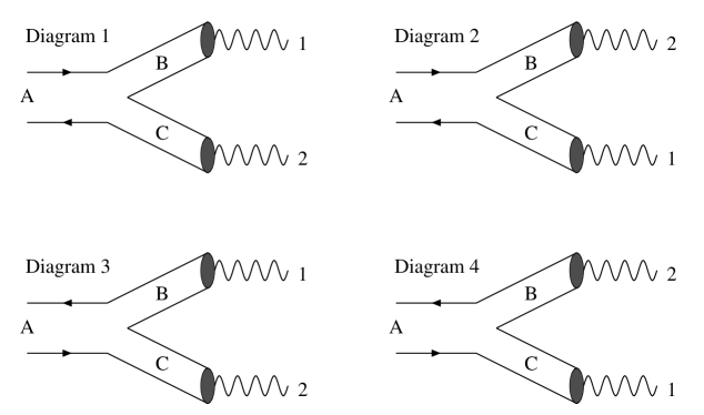
Figure 1: Diagrams constributing to the two photon decays of hybrid and conventional mesons. Right arrows indicate quarks, and left arrows antiquarks.

1 Overall Features of the Formalism

We work in the rest frame of the conventional or hybrid meson A, which couples to vector mesons B and C. These in turn each couples to photon 1 or 2 (see Fig. 1). A vector meson has a non–relativistic spin projection $M_{S}^{V}$ equal to the angular momentum projection $M_{J}^{i}$ of the photon $i$. The photons are at first assumed to be off–shell $q_{i}^{2}\neq 0$, and hence can be distinguished based on the square of their four–momenta. There are two ways of coupling the photons: with vector mesons B and C coupled to photons 1 and 2 respectively (called “Diagram 1”), and with B and C coupled to 2 and 1 respectively (“Diagram 2”). The hadronic kernel is unchanged in these two diagrams, except to the extent that B and C couple to different photons. This means that to obtain Diagram 2 from Diagram 1 we have to replace the momentum of vector meson B, denoted by $\bf{p_{B}}$, to $-\bf{p_{B}}$; and that we have to interchange $M_{S}^{B}$ and $M_{S}^{C}$. Replacing $\bf{p_{B}}$ by $-\bf{p_{B}}$ introduces a sign $(-1)^{L}$ for a decay amplitude in partial wave $L$.

Since the $Q\bar{Q}$ pair is assumed to be created with spin 1, the hadronic kernel will contain spin dependence ${\mbox{\boldmath$\sigma$}}=(\sigma_{x},\sigma_{y},\sigma_{z})$ in terms of Pauli matrices. We then take the overlap of the spin wavefunctions of A, B and C, and obtain in the language of refs. [7, 12] a spin dependence $Tr(A^{T}B{\mbox{\boldmath$\sigma$}}^{T}C)^{SM_{S}}$ in the amplitude. Here the spins of states A, B, or C are denoted by the appropriate matrix A, B, or C. $Tr(A^{T}B{\mbox{\boldmath$\sigma$}}^{T}C)^{SM_{S}}$ is found to change by $(-1)^{S_{A}+S_{B}+S_{C}+1}$ under exchange of $M_{S}^{B}$ and $M_{S}^{C}$ (see the Appendix of ref. [13]). Here $S_{A}$ is the spin of state A and $S_{B}=1=S_{C}$.

Since Diagram 2 and Diagram 1 are related by a sign $(-1)^{L}$, and the rule for exchange of $M_{S}^{B}$ and $M_{S}^{C}$, it follows that Diagram 2 = $(-1)^{S_{A}+S_{B}+S_{C}+1+L}$ Diagram 1. In the limit of adiabatically moving quarks, the $Q\bar{Q}$ spin for mesons are just those of the non–relativistic quark model. For hybrids the $Q\bar{Q}$ spin is 1 for $J^{PC}=(0,1,2)^{-+}$ and 0 for $1^{++}$ [6, 11]. By explicitly considering each two photon process discussed in this paper, we obtain that $(-1)^{S_{A}+S_{B}+S_{C}+1+L}$ is 1 for mesons (constructive interference) and $-1$ for hybrids (destructive interference). Hence for hybrids Diagrams 1 and 2 cancel. This yields a vanishing hybrid meson two photon coupling.

There is, however, something that has been left out of the above discussion. The meson propagator contains a term that links the $q_{i}^{2}$ of the photon to the vector meson mass $m_{V}$ (see Eq. 1). Each diagram is proportional to the product of the propagators of vector meson B and C. This means that if $q_{1}^{2}\neq q_{2}^{2}$, the symmetry under exchange of photon labels is broken if $m_{B}\neq m_{C}$. Hence two photon couplings of hybrid mesons are not exactly zero, but small. In the case of decays the photons are real, i.e. $q_{1}^{2}=0=q_{2}^{2}$, hybrid meson two photon decay widths are exactly zero.

In Diagrams 1 and 2, we have the quark of state A contained in B, and the antiquark in C. When B and C are distinguishable (which they are when they have different masses or flavours), there is a second possibility: the antiquark of state A can be contained in B, and the quark in C. These possibilities are denoted by Diagrams 3 and 4.

The same reasoning applied previously to the relationship between Diagrams 1 and 2 can also be applied to the relationship between Diagrams 3 and 4. We conclude that hybrid meson two photon couplings are small and decay widths vanish. This is the central claim of this paper.

2 Consistency Checks on the Formalism

Yang’s Theorem

Yang’s theorem states that total angular momentum $J_{A}=1$ states do not couple to two real photons. We explicitly check that this is satisfied.

Real photons can only be transversly polarized, so that $M_{S}^{V}=\pm 1$. For a $1^{++}$ meson this means that only $M_{S}^{A}=0$ contributes. In addition, it can be shown that $Tr(A^{T}B{\mbox{\boldmath$\sigma$}}^{T}C)^{SM_{S}}=0$ for $M_{S}^{A}=0,\;M_{S}^{B}=\pm 1,\;M_{S}^{C}=\mp 1$ if A has spin 1. Because a $1^{++}$ meson has spin 1 [6, 11], it follows that it does not couple to real photons, as required. A $1^{++}$ or $1^{-+}$ hybrid does not couple to real photons because all hybrid amplitudes vanish in this case.

By postulating that the coupling of a longitudinal photon to a vector meson is proportional to $f_{i}$ (Eq. 1), where ${f}_{i}\;(q_{i}^{2}=0)=0$, we can insure that real photons cannot be longitudinally polarized, and that Yang’s theorem is lifted when $q_{i}^{2}\neq 0$.

Bose Symmetry

When $M_{J}^{1}=M_{J}^{2}$ and $q_{1}^{2}=q_{2}^{2}$ the photons are identical. By Bose symmetry we expect their coupling to vanish if the process happens in odd wave, e.g. for $(0,1,2)^{-+}\rightarrow\gamma\gamma$. For $(0,2)^{-+}$ mesons Bose symmetry is explicitly protected by the fact that exchange $M_{J}^{1}\leftrightarrow M_{J}^{2}$ introduces a sign $(-1)^{S_{A}+S_{B}+S_{C}+1}$ which is odd (see previous section). But we know that $M_{J}^{1}=M_{J}^{2}$, so that exchange $M_{J}^{1}\leftrightarrow M_{J}^{2}$ trivially introduces an even sign. Thus the coupling vanishes. For hybrid $(0,1,2)^{-+}$ we already know that the amplitudes vanish when $q_{1}^{2}=q_{2}^{2}$.

Electric Charge

In a quark level picture of two photon decay widths [14, 15] $u\bar{u}\pm d\bar{d}\rightarrow\gamma\gamma$ is proportional to $((\frac{2}{3})^{2}\pm(-\frac{1}{3})^{2})^{2}$ due to the $u,d$ electric charges, yielding a width ratio $9:25$ for isospin $I=1\;:\;I=0$ states. Due to the fact that flavour is treated similarly in this formalism, we expect the same result. From Eqs. 3 and 7 (see below) $\;I=1:I=0\;=\;8{\cal R}_{\omega}^{2}:2(1+{\cal R}_{\omega}^{2})^{2}\;\approx\;9:25$, consistent with expectations.

The preceding checks are satisfied, as expected, independent of detailed dynamics. Having acquired confidence in the formalism, we proceed in the following sections to display detailed model calculations.

3 Intermediate Vector Mesons

The coupling strength of photon $i$ to vector meson V is defined by the dimensionless product of the vector meson dominance vertex and the vector meson propagator

$$V_{i}=\frac{-em_{V}^{2}{\cal R}_{V}}{2\gamma_{\rho}}\frac{1}{q_{i}^{2}-m_{V}^{2}}\;\left\{\begin{array}[]{cl}1&\mbox{transverse }i\\ {f}_{i}&\mbox{longitudinal }i\end{array}\right.\hskip 36.98866pt{\cal R}_{\rho}=1$$ (1)

where ${f}_{i}$ is a continuous function of $q^{2}_{i}$ such that ${f}_{i}\;(q_{i}^{2}=0)=0$. The constant $\gamma_{\rho}$ can be fitted from the $e^{+}e^{-}$ width of the $\rho$ meson. ${\cal R}_{V}$ parameterizes the ratio of the photon coupling amplitude for vector meson $V$ relative to that of the $\rho$ meson, and can be fitted from the $e^{+}e^{-}$ width of $V$.

We now investigate the relationship between Diagrams 1 and 3. They are related by the quark in A being contained in either B or C respectively. In the studies of hadronic decays [7, 16, 17] these diagrams have been shown [12] to be related by the sign $(-1)^{I_{A}+I_{B}+I_{C}+S_{A}+S_{B}+S_{C}+1+L+\Lambda}$, which always equals unity for allowed couplings. This implies that Diagrams 1 and 3 (and similarly Diagrams 2 and 4) are numerically identical. The angular momentum $\Lambda$ of the flux around A’s moving $Q\bar{Q}$ axis vanishes for mesons and equals $\pm 1$ for hybrids. The sign differs from that in section 1 because photons do not “know” about flavour and flux–tube degrees of freedom.

When B and C are not distinguishable (in mass and flavour), both Diagrams 1 and 3 are included in conventional studies of hadronic decay [7, 16, 17] since B and C can be distinguished based on their momenta. However, when B and C are intermediate states, they cannot be distinguished in this way. Hence only Diagrams 1 and 2 are included in this calculation for intermediate states $\rho^{0}\rho^{0},\;\omega\omega,\;\phi\phi,\;\psi\psi$, and not Diagrams 3 and 4.

When we calculate the square of the amplitude for the diagrams in Fig. 1, we obtain a common term which is independent of the $J^{PC}$ of state A, denoted by

$${\cal D}_{\pm}\equiv(Tr(AB^{T}C^{T})^{F}\;\frac{1}{2}(\mbox{Number of Diagrams})\;(\sum_{B,C}B_{1}C_{2}\pm B_{2}C_{1}))^{2}$$ (2)

where we group together the flavour overlap $Tr(AB^{T}C^{T})^{F}$, the various diagrams and the photon couplings. The summation in Eq. 2 refers to the sum over intermediate hadronic states B and C. The term inside the summation refers to the product of the $V_{i}$ for Diagram 1 added or subtracted to the product of the $V_{i}$ for Diagram 2. For conventional mesons we have addition and for hybrid mesons subtraction as discussed in section 1. If Diagrams 3 and 4 contributes, their contribution is the same as that of Diagrams 1 and 2, and is incorporated via the “Number of Diagrams” term in Eq. 2.

From Eq. 1

$$\sum_{B,C}B_{1}C_{2}+B_{2}C_{1} = 2\frac{\pi\alpha}{\gamma_{\rho}^{2}}\sum_{B,C}{\cal R}_{B}{\cal R}_{C}$$ (3)

$$\sum_{B,C}B_{1}C_{2}-B_{2}C_{1} = \frac{\pi\alpha}{\gamma_{\rho}^{2}}\sum_{B,C}{\cal R}_{B}{\cal R}_{C}{\cal F}_{BC}$$

$$\mbox{where }{\cal F}_{BC} \equiv ((1-\frac{q_{1}^{2}}{m_{B}^{2}})(1-\frac{q_{2}^{2}}{m_{C}^{2}}))^{-1}-((1-\frac{q_{2}^{2}}{m_{B}^{2}})(1-\frac{q_{1}^{2}}{m_{C}^{2}}))^{-1}$$ (4)

and we simplified Eq. 3 for real photons. Since ${\cal F}_{BC}=0$ for real photons, hybrid meson widths vanish. Equally, when $q_{1}^{2}=q_{2}^{2}$ the production amplitudes vanish. Hence hybrids are expected to be produced only if $q_{1}^{2}\neq q_{2}^{2}$, and even then with at least three orders of magnitude suppression (see Fig. 2 and section 4).

For meson two photon decays, the low–lying (G–parity allowed) hadronic intermediate states are included as

$$I=1: \rho\omega {\cal D}_{+}=(\frac{1}{\sqrt{2}}\;2\;2\frac{\pi\alpha}{\gamma_{\rho}^{2}}{\cal R}_{\omega})^{2}=8(\frac{\pi\alpha}{\gamma_{\rho}^{2}})^{2}{\cal R}_{\omega}^{2}$$

$$I=0: \rho\rho,\;\omega\omega {\cal D}_{+}=(\frac{1}{\sqrt{2}}\;1\;2\frac{\pi\alpha}{\gamma_{\rho}^{2}}(1+{\cal R}_{\omega}^{2}))^{2}=2(\frac{\pi\alpha}{\gamma_{\rho}^{2}})^{2}(1+{\cal R}_{\omega}^{2})^{2}$$

$$s\bar{s}: \phi\phi {\cal D}_{+}=(1\;1\;2\frac{\pi\alpha}{\gamma_{\rho}^{2}}{\cal R}_{\phi}^{2})^{2}=4(\frac{\pi\alpha}{\gamma_{\rho}^{2}})^{2}{\cal R}_{\phi}^{4}$$

$$c\bar{c}: \psi\psi {\cal D}_{+}=(1\;1\;2\frac{\pi\alpha}{\gamma_{\rho}^{2}}{\cal R}_{\psi}^{2})^{2}=4(\frac{\pi\alpha}{\gamma_{\rho}^{2}})^{2}{\cal R}_{\psi}^{4}$$ (5)

where each of the components of ${\cal D}_{+}$ in Eq. 2 is explicitly indicated. For two photon decays of hybrids the dominant intermediate states are included as

$$I=1: \rho_{R}\omega,\;\omega_{R}\rho {\cal D}_{-}=(\frac{1}{\sqrt{2}}\;2\;\frac{\pi\alpha}{\gamma_{\rho}^{2}}({\cal R}_{\rho_{R}}{\cal R}_{\omega}{\cal F}_{\rho_{R}\omega}+{\cal R}_{\omega_{R}}{\cal F}_{\omega_{R}\rho}))^{2}$$

$$I=0: \rho_{R}\rho,\;\omega_{R}\omega {\cal D}_{-}=(\frac{1}{\sqrt{2}}\;2\;\frac{\pi\alpha}{\gamma_{\rho}^{2}}({\cal R}_{\rho_{R}}{\cal F}_{\rho_{R}\rho}+{\cal R}_{\omega_{R}}{\cal R}_{\omega}{\cal F}_{\omega_{R}\omega}))^{2}$$

$$s\bar{s}: \phi_{R}\phi {\cal D}_{-}=(1\;2\;\frac{\pi\alpha}{\gamma_{\rho}^{2}}{\cal R}_{\phi_{R}}{\cal R}_{\phi}{\cal F}_{\phi_{R}\phi})^{2}$$

$$c\bar{c}: \psi_{R}\psi {\cal D}_{-}=(1\;2\;\frac{\pi\alpha}{\gamma_{\rho}^{2}}{\cal R}_{\psi_{R}}{\cal R}_{\psi}{\cal F}_{\psi_{R}\psi})^{2}$$ (6)

where the minus sign in ${\cal F}_{BC}$ explicitly incorporates the destructive interference derived in section 1. We choose the intermediate vector mesons in Eq. 3, involving radially excited states $\rho_{R},\;\omega_{R},\;\phi_{R}$ and $\psi_{R}$, for the following reasons. When $m_{B}\approx m_{C}$, as is the case for hybrid decays to two low–lying S–wave vector mesons, ${\cal F}_{BC}\sim m_{B}-m_{C}$ is small, suppressing the decay amplitude for these intermediate states by $\stackrel{{\scriptstyle<}}{{\scriptstyle\sim}}\frac{m_{\rho}-m_{\omega}}{m_{\rho_{R}}-m_{\omega}}=2\%$ relative to the modes listed in Eq. 3. In addition, for hybrid decays into low–lying S–wave vector mesons, the hadronic kernel is proportional to $(\frac{\beta_{B}^{2}-\beta_{C}^{2}}{\beta_{B}^{2}+\beta_{C}^{2}})^{2}$ in the flux–tube model [7] when S.H.O. wave functions with inverse radii $\beta_{B}$ and $\beta_{C}$ are used. This is zero for $\rho^{0}\rho^{0},\;\omega\omega,\;\phi\phi,\;\psi\psi$ and $\stackrel{{\scriptstyle<}}{{\scriptstyle\sim}}10^{-4}$ [12] for $\rho\omega$. Dominant contributions to two photon widths of hybrids are thus expected to come from intermediate states consisting of one radially excited (2S), D–wave or hybrid meson with one low–lying S–wave meson. Hybrid meson coupling to a photon is generally [18] believed to be suppressed, and at least in the non–relativistic limit, D–wave mesons are also coupled weakly to photons. Hence the choice of terms in Eq. 3 represents dominant intermediate states.

3.1 Parameters

Using the fact that the $e^{+}e^{-}$ width of a vector meson is $\frac{\pi\alpha^{2}}{3}\frac{m_{V}}{\gamma_{\rho}^{2}}{\cal R}_{V}^{2}$, we can obtain $\frac{\gamma_{\rho}^{2}}{4\pi}=0.507$ and

$${\cal R}_{\omega}=0.30\;\;\;{\cal R}_{\phi}=0.39\;\;\;{\cal R}_{\psi}=0.44\;\;\;{\cal R}_{\psi_{R}}=0.26$$ (7)

using experimental $e^{+}e^{-}$ widths and masses [19]. For the higher mass vector mesons, similar considerations using the $e^{+}e^{-}$ widths of ref. [20] show that the values of ${\cal R}_{V}$ derived are in substantial disagreement with theoretical expectations [21] (see Eq. 8) which may arise due to substantial mixing between 2S, 1D and hybrid in the physical states [8, 20]. Relativized quark models predict that

$${\cal R}_{\rho_{R}}=0.19\;\;\;{\cal R}_{\omega_{R}}=0.061\;\;\;{\cal R}_{\phi_{R}}=0.14$$ (8)

which we adopt.

4 Flux–tube Model Hadronic Kernel and Results

We adopt a hadronic decay model which predicts hybrid meson decays [22] by fixing parameters from known conventional meson decays, called the non–relativistic flux–tube model of Isgur and Paton [11]. In addition to providing absolute estimates for the hadronic kernel, this model reduces for S.H.O. wave functions [22] to the phenomenologically successful [23] ${}^{3}P_{0}$ decay model.

4.1 Meson Coupling

Table 1: Two photon theoretically predicted and experimentally observed [19] widths (in keV) of the lowest radially excited mesons of various $J^{PC}$ and flavour. When masses are not listed in ref. [19], their assumed values are listed (in MeV) in square brackets. Due to details of phase space conventions hadronic decay models can also allow $\gamma_{0}=0.53$ [23], and hence the theoretical predictions listed can be $(0.53/0.39)^{2}\approx 2$ times bigger. Light pseudoscalars are well described [26] by chiral dynamics and are not quoted. The broad nature of the $f_{0}(1370)$ has not been taken account of. We took $\beta_{A}=$ 0.33, 0.40, 0.50, 0.31, 0.39, 0.47, 0.45, 0.57 GeV for $\{a_{2},a_{0},f_{2},f_{0}(1370)\},\;\{f_{2}^{{}^{\prime}},f_{0}(1710),\eta_{2}(1875)\},\;\{\chi_{c2},\chi_{c0}\},\;\pi_{2},\;\pi,\;\{\eta_{u\bar{u}},\eta_{s\bar{s}}\},\;\eta_{c2},\;\eta_{c}$. Also $\beta=$ 0.39, 0.47, 0.57 GeV for $u\bar{u},\;s\bar{s},\;c\bar{c}$. Theory error estimates are obtained by varying $\beta_{A},\beta$ in the same direction within $0.05$ GeV of the mean values above. $\star$ Ref. [32]. $\P$ Ref. [33]. $\dagger$ Ref. [29]. $\ddagger$ Ref. [34]. $\amalg$ Ref. [21].

		$0^{-+}$	$0^{++}$	$2^{++}$	$2^{-+}$
		$\pi$	$a_{0}[1450]$ ⋆	$a_{2}$	$\pi_{2}(1670)$
$I=1$	Th	$-\;$	$0.7\pm 0.5$	$0.9\pm 0.1$	$0.1{\lower 3.01385pt\hbox{$\;\stackrel{{\scriptstyle\textstyle+0.3}}{{-0.1}}\;$}}$
	Ex	$7.29\pm 0.19\;\mbox{eV}$	$-$	$1.04\pm 0.09$	$1.13\pm 0.24$
	Ex			$0.96\pm 0.13$ $\P$	$<0.19$ $\P$
			$f_{0}(1370)$	$f_{2}$	$\eta_{2}[1645]$ †
$I=0$	Th		$-$	$2.8\pm 0.2$	$0.4{\lower 3.01385pt\hbox{$\;\stackrel{{\scriptstyle\textstyle+0.7}}{{-0.3}}\;$}}$
	Ex		$5.4\pm 2.3$	$2.8\pm 0.4$	$-$
				$f_{2}^{{}^{\prime}}$
$s\bar{s}$	Th			$0.17\pm 0.01$
	Ex			$0.105\pm 0.017$
		$\eta_{c}$	$\chi_{c0}$	$\chi_{c2}$	$\eta_{c2}[3840]$ ∐
$c\bar{c}$	Th	$7.2\pm 0.2$	$4.1\pm 0.4$	$2.2\pm 0.1$	$2.0\pm 0.3$
	Ex	$7.5\pm 1.5$	$4.0\pm 2.8$	$0.37\pm 0.17$	$-$
	Ex	$4.3\pm 1.4$ ‡	$1.7\pm 0.8$ ‡	$0.7\pm 0.3$ ‡

The analytic expressions for a meson coupling to two vector mesons in the flux–tube model, with ${}^{3}P_{0}$ pair creation dynamics and non–relativistically moving quarks, is identical [22] to the ${}^{3}P_{0}$ model [16] in the case of S.H.O. wave functions. This is true if we make the identification $\gamma_{0}=\frac{a\tilde{c}}{9\sqrt{3}}\frac{1}{2}A^{0}_{00}\sqrt{\frac{fb}{\pi}}\;(1+\frac{fb}{2\beta^{2}})^{-1}$ for the ${}^{3}P_{0}$ model pair creation constant, where the flux–tube model constants $f=1.1,\;b=0.18\;GeV^{2}$, $A^{0}_{00}=1.0$, $\tilde{c}$ and $a$ are defined in refs. [7, 22, 24]. It is also assumed that $\beta_{B}=\beta_{C}\equiv\beta$. We set $\gamma_{0}=0.39$ for $\beta=0.4$ GeV, in accordance with meson decay phenomenology [16, 23]. The hadronic kernel is completely specified, and can be calculated using ref. [22]. The sum over total angular momentum projection of the squares of the helicity amplitudes $\sum_{M_{J}^{A},M_{S}^{B},M_{S}^{C}}|{\cal M}|^{2}$ is (for various $J^{PC}$)

$$0^{-+} : \hskip 8.5359pt{\varsigma}\;({\bf p}_{B}(\beta^{2}_{A}+\beta^{2}))^{2}$$

$$0^{++} : \hskip 8.5359pt{\varsigma}\;\frac{1}{3}(\frac{\beta_{A}}{{2\beta^{2}_{A}+\beta^{2}}})^{2}\;[2({\varsigma_{1}}-{\varsigma_{2}})^{2}+{f}_{1}^{2}{f}_{2}^{2}({\varsigma_{1}}+{\varsigma_{2}})^{2}]$$

$$1^{++} : \hskip 8.5359pt{\varsigma}\;(\frac{\beta_{A}}{{2\beta^{2}_{A}+\beta^{2}}})^{2}({f}_{1}^{2}+{f}_{1}^{2}){\varsigma_{2}}^{2}$$

$$2^{++} : \hskip 8.5359pt{\varsigma}\;\frac{1}{3}(\frac{\beta_{A}}{{2\beta^{2}_{A}+\beta^{2}}})^{2}\;[28{\varsigma_{1}}^{2}-8{\varsigma_{1}}{\varsigma_{2}}+4{\varsigma_{2}}^{2}+(3({f}_{1}^{2}+{f}_{2}^{2})+2{f}_{1}^{2}{f}_{2}^{2})\;(2{\varsigma_{1}}-{\varsigma_{2}})^{2}]$$

$$2^{-+} : \hskip 8.5359pt{\varsigma}\;\frac{4}{3}(\frac{{\bf p}_{B}\beta_{A}^{2}}{({2\beta^{2}_{A}+\beta^{2}})^{2}})^{2}\;[(2{\varsigma_{1}}-{\varsigma_{2}})^{2}+3({f}_{1}^{2}+{f}_{2}^{2}){\varsigma_{1}}^{2}]$$ (9)

$$\hskip 28.45274pt{\varsigma}\equiv{\cal D}_{+}\;2^{8}\pi^{\frac{3}{2}}\gamma_{0}^{2}\;\frac{\beta_{A}^{3}}{({2\beta^{2}_{A}+\beta^{2}})^{5}}\exp(-\frac{{\bf p}_{B}^{2}}{2({2\beta^{2}_{A}+\beta^{2}})})$$

$$\hskip 28.45274pt{\varsigma_{1}}\equiv\beta^{2}\;({2\beta^{2}_{A}+\beta^{2}})\hskip 28.45274pt{\varsigma_{2}}\equiv{\bf p}_{B}^{2}\;(\beta_{A}^{2}+\beta^{2})$$

where $\beta_{A}$ is the S.H.O. wave function inverse radius of state A. In Eq. 4.1 we explicitly seperate longitudinal and transverse contributions: Expressions with one ${f}_{i}^{2}$ correspond to photon $i$ being longitudinal, and those containing ${f}_{1}^{2}{f}_{2}^{2}$ have both photons longitudinal.

Using the parameters of refs. [7, 12], and with the help of Eqs. 3, 4.1 and 18 for real photons, we obtain the meson width predictions of Table 1. No parameter fitting has been done, and it is encouraging that the amplitudes roughly correspond to experimental values, establishing the validity of the model. There can, however, be substantial sensitivity if $\beta_{A},\beta$ is varied, especially near nodes in the amplitude.

Within this paper, it is sufficient to check the overall consistency of the approach. More detailed work would have to take into account relativistic corrections, which are known to be substantial [14, 15] at least in quark model approaches, and will have to fit $\gamma\gamma$ decays contingent on the corresponding hadronic $VV$ decays fitting experiment. The results in Table 1 complement quark model [14, 15] and quark model with vector meson dominance [15] approaches. These can be shown to be related to each other [15], motivating vector meson dominance at the quark level.

4.2 Hybrid Production

The flux–tube model predicts the hybrid pair creation constant $\tilde{\gamma}_{0}=\kappa\sqrt{b}\gamma_{0}\;(1+\frac{fb}{2\beta^{2}})^{-1}$ for S.H.O. meson wave functions, in terms of the meson pair creation constant, where the model constant $\kappa=0.9$ is defined in refs. [7, 22, 24]. $\sum_{M_{J}^{A},M_{S}^{B},M_{S}^{C}}|{\cal M}|^{2}$ for various $J^{PC}$ is (see Appendix B)

$$0^{-+} : \hskip 8.5359pt0$$

$$1^{++} : \hskip 8.5359pt{\varrho}\;2\;[4(\breve{g}_{0}+\breve{g}_{2})^{2}+({f}_{1}^{2}+{f}^{2}_{2})(2\breve{g}_{0}-\breve{g}_{2})^{2}]$$

$$1^{-+} : \hskip 8.5359pt{\varrho}\;9\breve{g}_{1}^{2}\;[{f}_{1}^{2}+{f}^{2}_{2}+2{f}_{1}^{2}{f}^{2}_{2}]$$

$$2^{-+} : \hskip 8.5359pt{\varrho}\;9\breve{g}_{1}^{2}\;[8+{f}_{1}^{2}+{f}^{2}_{2}]$$ (10)

$$\hskip 28.45274pt{\varrho}\equiv{\cal D}_{-}\;\frac{8}{9}\;\tilde{\gamma}_{0}^{2}\frac{\pi\beta_{A}^{3+2\delta}}{\Gamma(\frac{3}{2}+\delta)}$$

$$\hskip 28.45274pt\breve{g}_{n}=\int_{0}^{\infty}dr\;r^{2+\delta}\;j_{n}(\frac{1}{2}p_{B}r)\;\exp(-(2\beta_{A}^{2}+\beta^{2})\frac{r^{2}}{4})$$

where $\delta=0.62$ [7], and $j_{n},\;\Gamma$ are the spherical Bessel and gamma functions. Utilizing Eqs. 4, 4.2 and 18 we obtain the production strengths of hybrid mesons in Table 2 by first estimating the widths $\Gamma_{+}$ for constructive interference, and then correcting for the suppression caused by destructive interference.

Figure 2: The “lifting of suppression”. This is the ratio of ${\cal D}_{-}$ (Eq. 3) to what would have been obtained for ${\cal D}_{-}$ if the sign of ${\cal F}_{BC}$ in Eq. 4 was positive. The ratio indicates the size of the actual destructive interference in hybrid meson two photon coupling, relative to the size of hybrid meson two photon coupling that would result in the hypothetical case of constructive interference. The lifting of suppression is plotted as a function of $Q\equiv\sqrt{-q_{1}^{2}}$ ($q_{1}^{2}\leq 0$) where $q_{2}^{2}=0$. The case when one of the photon momenta is real (in this case $q_{2}$) yields the maximal lifting of suppression as long as the physical production constraint $q_{i}^{2}\leq 0$ holds for the other photon. The graphs from highest to lowest lifting of suppression (at $Q=1$ GeV) are for $I=0,\;I=1,\;s\bar{s}$ and $c\bar{c}$ flavours. The $c\bar{c}$ lifting of suppression is maximal at $\approx 3.4$ GeV and decreases at higher $Q$.

Table 2: Predicted upper bounds on the two photon “widths” $\Gamma_{max}$ (in eV) of hybrids of various $J^{PC}$ and flavour. These are obtained by multiplying the two photon widths $\Gamma_{+}$ (in eV) that would have been attained if the sign in ${\cal F}_{BC}$ in Eq. 4 was positive instead of negative by the maximal “lifting of suppression” in Fig. 2, which is 2.3%, 2.4%, 1.6%, 0.19% for $I=1,\;I=0,\;s\bar{s},\;c\bar{c}$ respectively. $\Gamma_{max}$ is hence not a decay width, since the decay widths of hybrid mesons are zero, but indicates the maximal production strength of hybrid mesons in two photon processes. For $u\bar{u},\;s\bar{s},\;c\bar{c}$ we use respectively $\beta_{A}=0.27,0.30,0.30$ GeV and $\beta=0.37,0.50,0.57$ GeV. Hybrid masses are those of ref. [7] i.e. $\approx$ 1.9, 2.1, 4.3 GeV for $u\bar{u},\;s\bar{s},\;c\bar{c}$ hybrids.

		$I=1$	$I=0$	$s\bar{s}$	$c\bar{c}$
$\Gamma_{max}$	$2^{-+}$	1	3	0.3	0.1
	$1^{++}$	0.4	1	0.2	0.03
$\Gamma_{+}$	$2^{-+}$	40	140	20	50
	$1^{++}$	20	60	10	20

5 Phenomenology and Conclusions

We have exhibited a formalism to discuss two photon decays of hybrid and conventional mesons through intermediate hadronic states. The formalism respects Bose symmetry and ensures the consistency requirement that $J=1$ states do not couple to two real photons. These are direct consequences of the creation of the $Q\bar{Q}$ pair with spin 1. The formalism also preserves the naïve expectation for the ratio of $I=1$ and $I=0$ amplitudes of $9/25$ for both mesons and hybrids demanded by the difference between up and down quark electric charges, in accordance with experiment.

Microscopic decay models [25] have found either dominant scalar confining interaction ${}^{3}P_{0}$, subdominant transverse one gluon exchange ${}^{3}S_{1}$ or highly suppressed colour Coulomb one gluon exchange ${}^{3}P_{0}$, i.e. spin 1, pair creation for conventional mesons. If we assume that these decay mechanisms also dominate for hybrids, we have demonstrated that for both ${}^{3}P_{0}$ and ${}^{3}S_{1}$ pair creation Yang’s theorem and Bose symmetry are satisfied, and two photon decays of hybrid mesons vanish. These results are independent of detailed dynamics, but depends on the valence quarks moving non–relativistically as the only “quenched” quarks relevant to the connected decay, the absense of final state interactions, the spin assignment of a hybrid being that of the adiabatic limit [6, 11], and the photons coupling via intermediate vector mesons. In the case of either the pair being created with spin 0 instead of spin 1, or the hybrid spin assignments being the opposite to that of refs. [6, 11] hybrid widths may be non–vanishing. We caution that the breaking of assumptions made to derive the small hybrid production strengths $\stackrel{{\scriptstyle<}}{{\scriptstyle\sim}}0.03-3$ eV (Table 2) can lead to more significant production. However, hybrid $\gamma\gamma$ widths are also small in a relativistic model [15], being $O(\alpha_{S})$ suppressed relative to meson $\gamma\gamma$ widths.

Production strengths for hybrids are seen from Tables 1 and 2 to be three orders of magnitude lower than for mesons, and can hence be unpromising experimentally. This is especially relevant to the only low–lying exotic $J^{PC}$ accessable to $\gamma\gamma$, i.e. $1^{-+}$, where there is additional suppression in the formalism due to the photon coupling being restricted to longitudinal polarizations (see Eq. 4.2). Given the assumptions made, the main signature would be vanishing production for $q^{2}_{1}=q^{2}_{2}$.

Two photon collisions can be strong discriminators in favour of the non–gluonic components of a physical state. We have demonstrated this in a specific context for hybrid mesons, and it is usually believed to be the case for glueballs [26]. For non–exotic $J^{PC}$ physical states are expected [8] to have both hybrid and conventional $Q\bar{Q}$ wave function components. Babar, Cleo II, LEP2 and LHC experiments should thus have considerable value in isolating substantial non–gluonic components in mixed states. $f_{0}(1500),\;f_{J}(1710)$ [5, 15], $\rho(1450),\;\rho(1700)$, $\omega(1420),\;\omega(1600)$ [8, 20], $\psi(4040)$ and $\psi(4160)$ [18, 27] have recently been suggested to be mixed. In mixed states $\;\sin\phi\;|\mbox{non}-Q\bar{Q}\rangle+\cos\phi\;|Q\bar{Q}\rangle\;$ and $\;\cos\phi\;|\mbox{non}-Q\bar{Q}\rangle-\sin\phi\;|Q\bar{Q}\rangle\;$ $\;\gamma\gamma$ collisions should isolate components proportional to $\cos^{2}\phi$ and $\sin^{2}\phi$ respectively, manifestly indicating the extent of non–gluonic mixing by the strength of the two peaks appearing.

In the case of pure hybrid candidates with non–exotic $J^{PC}$, $\gamma\gamma$ collisions offer the unique opportunity to isolate and clearly distinguish the quarkonium partner, e.g. for the 1.8 GeV $0^{-+}$ isovector observed at VES [28]. Here the distinction is especially pronounced since $0^{-+}$ hybrid meson two photon production always vanishes in the flux–tube model (see Appendix A). VES possibly sees two states, one a hybrid and the other a second radially excited $\pi$ [8, 9]. This should in principle show up as two peaks in hadronic decay channels. Unfortunately, theoretical predictions of hadronic decays of radially excited $Q\bar{Q}$ are highly sensitive to parameter variations [8], making comparisons to hybrid decays difficult. Even though no radially excited $Q\bar{Q}$ has been observed thus far in $\gamma\gamma$, it is within this formalism an exceptionally clean “higher quarkonium” production mechanism, and a second radially excited $\pi$ may show up as one unambigous peak. Since the $\rho\omega$ decay of $0^{-+}$ has been observed [28], we expect the $\gamma\gamma$ collisions production of the quarkonium component of $0^{-+}$ via intermediate $\rho,\omega$.

Recently, an isoscalar $2^{-+}$ state at 1.875 GeV has been seen [29], which appears to be the same as a state reported previously by the Crystal Ball and Cello Collaborations [30]. In addition, an isovector $2^{-+}$ at 1.8 GeV has been reported by a number of collaborations [8], most recently VES [28]. Detailed analysis [8] of these states leave it unsure whether they are radially excited D–wave $Q\bar{Q}$ or hybrids. In addition, VES reported a 2.2 GeV isovector $2^{-+}$ [28], which has characteristics inconsistent with expectations for a hybrid [7]. We suggest that $\gamma\gamma$ collisions should be able to distinguish the non–gluonic content of these states in the $1.8-2.2$ GeV region. The $\pi_{2}(1670)$ has been produced in $\gamma\gamma$ collisions by the Crystal Ball and Cello Collaborations [31]. However, in both of these experiments there are suggestive hints that there may be an isovector contribution around 1.8 GeV, since the data appear to be skewed towards the higher masses relative to simple Breit Wigner and PDG values. Moreover, one expects that the isoscalar $2^{-+}$ may also appear in $\gamma\gamma$ collisions, since $\Gamma(\gamma\gamma\rightarrow I=0)$ $>$ $\Gamma(\gamma\gamma\rightarrow\ I=1)$. Evidence for the isoscalar has been presented in ref. [30].

We have seen that two photon collisions act as powerful discriminators between gluonic and non–gluonic components and may considerably advance the isolation of gluonic forms of matter, underlining the experimental potential of two photon physics.

Helpful discussions with T. Barnes, A. Donnachie, J. Forshaw, S.A. Sadovsky, P. Sutton, R. Williams and especially F.E. Close are acknowledged.

Appendix A Appendix: Why Hybrid $0^{-+}$ Coupling to Two Vector Mesons Vanishes

A general decay configuration can be rotated to a space fixed configuration by using Appendix 1 of ref. [11]

$$\psi({\bf r}_{H})={\cal D}^{L_{H}}_{M_{L}^{H}\Lambda_{H}}(\phi,\theta,\alpha)\;\psi({\bf r}_{H}^{f})$$ (11)

where state H has orbital angular momentum $L_{H}$, orbital angular momentum projection $M_{L}^{H}$, angular momentum $\Lambda_{H}$ around the $Q\bar{Q}$ axis ${\bf r}_{H}$, and ${\bf r}_{H}^{f}$ indicates the axis in the fixed configuration. H labels any of the states A, B or C. Similarly, for the decay operator

$${\mbox{\boldmath$\sigma$}}\cdot{\mbox{\boldmath$\nabla$}}=\sigma^{\sigma}\nabla_{\sigma}={\cal D}^{1\ast}_{\sigma\mu}(\phi,\theta,\alpha)\;\sigma^{\sigma}\nabla_{\mu}^{f}$$ (12)

where $\sigma$ denotes spherical basis coordinates.

Hence, focussing on the $\theta,\phi$ dependence of the flux–tube model decay amplitude [7] $\propto\;\langle BC|{\mbox{\boldmath$\sigma$}}\cdot{\mbox{\boldmath$\nabla$}}|A\rangle$, we have

$$\int\sin\theta\;d\theta\;d\phi\;d\alpha\;{\cal D}^{L_{A}}_{M_{L}^{A}\Lambda_{A}}(\phi,\theta,\alpha)\;{\cal D}^{1\ast}_{\sigma\mu}(\phi,\theta,\alpha)\;{\cal D}^{L_{B}\ast}_{M_{L}^{B}\Lambda_{B}}(\phi,\theta,\alpha)\;{\cal D}^{L_{C}\ast}_{M_{L}^{C}\Lambda_{C}}(\phi,\theta,\alpha)\;e^{\frac{i}{2}{\bf p}_{B}\cdot{\bf r}}$$ (13)

where the fixed configuration has been suppressed. On $\phi$–integration the integral is only non–zero when $M_{L}^{A}=\sigma+M_{L}^{B}+M_{L}^{C}$ which indicates conservation of angular momentum projection. Similarly, on $\alpha$–integration, $\mu=\Lambda_{A}-\Lambda_{b}-\Lambda_{C}$, which indicates that pair creation absorbs the angular momentum in the fixed configuration.

For hybrid $0^{-+}\leftrightarrow VV$ we note that $L_{B}=L_{C}=0$, and $M_{L}^{A}=\sigma$ by the first conservation rule. Eq. 13 thus becomes

$${\cal M}_{M_{L}^{A}}\;({\bf p}_{B})\sim\int\sin\theta\;d\theta\;d\phi\;{\cal D}^{L_{A}}_{M_{L}^{A}\Lambda_{A}}(\phi,\theta,-\phi)\;{\cal D}^{1\ast}_{M_{L}^{A}\mu}(\phi,\theta,-\phi)\;e^{\frac{i}{2}{\bf p}_{B}\cdot{\bf r}}$$ (14)

where we adopted the convention of ref. [11], setting $\alpha=-\phi$ without loss of generality. Note that when ${\bf p}_{B}\rightarrow-{\bf p}_{B}$ Eq. 14 becomes

$${\cal M}_{M_{L}^{A}}\;(-{\bf p}_{B})\sim\int\sin\theta\;d\theta\;d\phi\;{\cal D}^{L_{A}}_{-M_{L}^{A}\Lambda_{A}}(\phi,\theta,-\phi)\;{\cal D}^{1\ast}_{-M_{L}^{A}\mu}(\phi,\theta,-\phi)\;e^{\frac{i}{2}{\bf p}_{B}\cdot{\bf r}}$$ (15)

where we exchanged variables ${\bf r}\rightarrow-{\bf r},\;\theta\rightarrow\pi-\theta,\phi\rightarrow\phi+\pi$ and used a property of the ${\cal D}$–functions. It follows that ${\cal M}_{0}$ and ${\cal M}_{1}+{\cal M}_{-1}$ are invariant under ${\bf p}_{B}\rightarrow-{\bf p}_{B}$. But from simple Clebsch–Gordon coefficients for $0^{-+}\leftrightarrow VV$ we have that the $M_{J}^{A}=0,\;M_{J}^{B}=\pm 1,\;M_{J}^{C}=\mp 1$ amplitude is $-\frac{1}{\sqrt{2}}{\cal M}_{0}$ and the $M_{J}^{A}=0,\;M_{J}^{B}=0,\;M_{J}^{C}=0$ amplitude is $\frac{1}{\sqrt{2}}({\cal M}_{1}-{\cal M}_{0}+{\cal M}_{-1})$, both of which are accordingly invariant under ${\bf p}_{B}\rightarrow-{\bf p}_{B}$. But since $0^{-+}\leftrightarrow VV$ is a P–wave decay the amplitude should be odd under ${\bf p}_{B}\rightarrow-{\bf p}_{B}$. Hence the amplitude, and also the production and decay $0^{-+}\leftrightarrow VV$ vanishes.

To derive vanishing $0^{-+}\leftrightarrow VV$, we assumed non–relativistically moving valence quarks, with hybrid $0^{-+}$ having the spin assignment of refs. [6, 11] and decaying via ${}^{3}P_{0}$ OZI allowed pair creation. The argument does not go through for ${}^{3}S_{1}$ pair creation.

Appendix B Appendix: Hybrid $\rightarrow$ 2S + 1S Mesons

The decay amplitude for $hybrid\rightarrow 1S+1S$ was displayed in Eq. 21 of ref. [7]. The amplitude for $hybrid\rightarrow 2S+1S$ can be obtained from it by noting that the 2S S.H.O. wave function equals

$$\psi_{2S}(r)=2\sqrt{\frac{2}{3}}\beta_{B}^{2}\;\frac{d}{d\beta_{B}^{2}}\psi_{1S}(r)$$ (16)

The derivative operator can now be pulled in front of the overall decay amplitude (Eq. 3 of ref. [7]) and can hence be applied to the $hybrid\rightarrow 1S+1S$ amplitude (Eq. 21 of ref. [7]). Noting that the amplitude for hybrid $\rightarrow$ 1S + 1S is proportional to $\Delta=\beta_{B}^{2}-\beta_{C}^{2}$, we first perform the differentiation and then set $\beta_{B}=\beta_{C}$ as a first orientation. Doing so sets $\Delta=0$, so the only contributing term will be from the derivative acting on $\Delta$. This yields a $hybrid\rightarrow 2S+1S$ amplitude of

$$2\sqrt{\frac{2}{3}}\beta_{B}^{2}\times(\;\mbox{Eq. 21 of ref. \cite[cite]{[\@@bibref{}{page95light}{}{}]}}\;)/\Delta$$ (17)

when we restrict $\beta_{B}=\beta_{C}$.

Appendix C Appendix: Width and Production Cross–Section

Real photons can be distinguished according to the hemisphere in which they are observed in an experimental apparatus, thus only appearing in a solid angle $2\pi$, leading to the width relation

$$\Gamma=\frac{1}{2J_{A}+1}\int(2\pi)^{4}\;\delta^{4}(q_{1}+q_{2})\;\frac{d^{3}q_{1}}{(2\pi)^{3}}\frac{d^{3}q_{2}}{(2\pi)^{3}}\sum_{M_{J}^{A},M_{S}^{B},M_{S}^{C}}|{\cal M}|^{2}$$ (18)

$$=\frac{m_{A}^{2}}{16\pi(2J_{A}+1)}\sum_{M_{J}^{A},M_{S}^{B},M_{S}^{C}}|{\cal M}|^{2}$$

where $m_{A}$ is the mass of state A.

References

- [1]
- [2] S.A. Sadovsky, Proc. of HADRON’95 (Manchester, 1995), p. 289, eds. M.C. Birse et al.
- [3] K. Hencken, D. Trautmann, G. Baur, Z. Phys. C68 (1995) 473.
- [4] M. Feindt, Proc. of HADRON’95 (Manchester, 1995), p. 303, eds. M.C. Birse et al.
- [5] F.E. Close, C. Amsler, Phys. Rev. D53 (1996) 295; D. Weingarten, Proc. of Workshop on Continuous Advances in QCD (Minneapolis, 1996), hep-ph/9607212.
- [6] C. Michael et al., Nucl. Phys. B347 (1990) 854; Phys. Lett. B142 (1984) 291; Phys. Lett. B129 (1983) 351; Liverpool Univ. report LTH-286 (1992), Proc. of the Workshop on QCD : 20 Years Later (Aachen, 9–13 June 1992); Phys.Rev. D54 6997.
- [7] F.E. Close, P.R. Page, Nucl. Phys. B443 (1995) 233; Phys. Rev. D52 (1995) 1706.
- [8] T. Barnes, F.E. Close, P.R. Page, E. Swanson, MC-TH-96/21, ORNL-CTP-96-09, RAL-96-039, hep-ph/9609339, to be published in Phys. Rev. D; F.E. Close, P.R. Page, “How to distinguish Hybrids from Radial Quarkonia”, RAL-97-002, MC-TH-96/31, hep-ph/9701425.
- [9] P.R. Page, Proc. of PANIC’96 (Williamsburg, 1996), ed. C. Carlson (1996).
- [10] J. Babcock, J.L. Rosner, Phys. Rev. D14 (1976) 1286; M. Tanimoto, Phys. Lett. B116 (1982) 198.
- [11] N. Isgur, J. Paton, Phys. Lett. 124B (1983) 247; Phys. Rev. D31 (1985) 2910.
- [12] P.R. Page, D. Phil. thesis, Univ. of Oxford (1995).
- [13] P.R. Page, hep-ph/9611375, MC-TH-96/26.
- [14] T. Barnes et al., Phys. Rev. D45 (1992) 232; ORNL-CTP-96-04, hep-ph/9605278.
- [15] F.E. Close, Z. Li, Z. Phys. C54 (1992) 147; Phys. Rev. D43 (1991) 2161.
- [16] R. Kokoski, N. Isgur, Phys. Rev. D35 (1987) 907.
- [17] N. Isgur, R. Kokoski, J. Paton, Phys. Rev. Lett. 54 (1985) 869.
- [18] S. Ono et al., Z. Phys. C26 (1984) 307; Phys. Rev. D34 (1986) 186.
- [19] Particle Data Group, Phys. Rev. D54 (1996) 1.
- [20] A.B. Clegg, A. Donnachie, Z. Phys. C62 (1994) 455.
- [21] S. Godfrey, N. Isgur, Phys. Rev. D32 (1985) 189.
- [22] P.R. Page, Nucl. Phys. B446 (1995) 189.
- [23] P. Geiger, E.S. Swanson, Phys. Rev. D50 (1994) 6855.
- [24] N. Dowrick, J. Paton, S. Perantonis, J. Phys. G13 (1987) 423; S.J. Perantonis, D. Phil. thesis, Univ. of Oxford (1987).
- [25] E.S. Ackleh, T. Barnes, E.S. Swanson, ORNL-CTP-96-03, hep-ph/9604355.
- [26] C. Berger, W. Wagner, Phys. Rep. 146 (1987) 1.
- [27] F.E. Close, P.R. Page, Phys. Lett. B366 (1995) 323.
- [28] D.V. Amelin et al. (VES Collab.), Phys. Lett. B356 (1995) 595; Jad. Fiz. 59 (1996) 1021; D.I. Ryabchikov, Proc. of HADRON’95 (Manchester, 1995), eds. M.C. Birse et al.; A.M. Zaitsev, Proc. of ICHEP (1994), p. 1409, eds. P. Bussey et al.; A.M.Zaitsev (VES Collab.), Proc. of ICHEP’96 (Warsaw, 1996).
- [29] C. Amsler et al. (Crystal Barrel Collab.), “Evidence for two isospin zero mesons at 1645 and 1875 MeV” and “Study of at 1200 MeV/c”.
- [30] K. Karch et al. (Chrystal Ball Collab.), Z. Phys. C54 (1992) 33; M. Feindt, Proc. of ICHEP (Singapore, 1990), p. 537.
- [31] D. Antreasyan et al. (Chrystal Ball Collab.), Zeit. Phys. C48 (1990) 561; H.-J. Behrend et al. (Cello Collab.), Zeit. Phys. C46 (1990) 583.
- [32] C. Amsler et al., Phys. Lett. B333 (1994) 277.
- [33] H. Albrecht et al. (ARGUS Collab.), DESY-96-112.
- [34] V. Savinov, R. Fulton, Proc. of PHOTON’95 (Sheffield, 1995) , p. 197, eds. D.J. Miller et al..