Freiburg–THEP 96/14

July 1996

Two–loop effects of enhanced electroweak strength in the Higgs sector
Adrian Ghinculov

Albert–Ludwigs–Universität Freiburg, Fakultät für Physik
Hermann–Herder Str.3, D-79104 Freiburg, Germany

The selfcoupling of the Higgs field grows with the mass of the Higgs particle and induces potentially large radiative corrections in the electroweak model. The technical aspects of performing multiloop calculations in the massive case are discussed briefly. I review the status of two–loop calculations of radiative corrections of enhanced electroweak strength which are relevant for the Higgs physics. I discuss the relevance of the existing results with respect to heavy Higgs searches at future colliders and their implications regarding the validity range of perturbation theory.

Abstract

The selfcoupling of the Higgs field grows with the mass of the Higgs particle and induces potentially large radiative corrections in the electroweak model. The technical aspects of performing multiloop calculations in the massive case are discussed briefly. I review the status of two–loop calculations of radiative corrections of enhanced electroweak strength which are relevant for the Higgs physics. I discuss the relevance of the existing results with respect to heavy Higgs searches at future colliders and their implications regarding the validity range of perturbation theory.

1 Introduction

The Higgs resonance required by the simplest version of a spontaneous electroweak symmetry breaking sector has eluded so far a direct detection. Indirect measurements of the Higgs mass still give rather loose bounds because of screening of the Higgs effects in low energy radiative corrections. In fact, a minimal Higgs with a mass of the order of 1 TeV is not excluded by the available data [1]. Still, the possibility of a heavy Higgs boson raises both theoretical and phenomenological problems because the selfinteraction of the Higgs field increases with the Higgs mass.

How does the Higgs sector behave in the strong coupling regime? This is an interesting question for which no definite answer exists yet. A number of approaches were proposed, although each has its own problems. An idea suggested long time ago by Veltman implies the formation of bound states of weak bosons which would behave like Higgs bosons with enhanced couplings to the vector bosons and to themselves [2]. For gaining insight into the behaviour of the Higgs sector at large selfcouplings, the nonperturbative $1/N$ expansion technique was developed. These models can be solved easily at leading order, and reveal for instance an interesting relation between the Higgs mass and width which deviates from the perturbative result for large couplings [3]. In particular, the Higgs mass saturates at a value of the order of 900 GeV when the quartic coupling is increased. Unfortunately, calculations beyond the leading order in the $1/N$ expansion are technically extremely difficult [4]. Also these models suffer of pathologies associated with the possible triviality of the $\phi^{4}$ theory when treated as renormalized fundamental theories. These problems show up in the presence of tachyons in the spectrum of the theory at leading order, and lead to problems in the higher orders of the $1/N$ expansion. To avoid this kind of inconsistencies, one can treat the theory as an effective theory by including explicitly a cutoff [5].

Setting upper bounds on the Higgs mass by requiring that the Higgs boson mass be lower than the triviality scale was attempted by lattice calculations [6]. These results must be interpreted with caution because the bounds obtained are regularization dependent – for instance they vary with the geometry of the lattice [7]. On the other hand, the top quark may play quantitatively a rôle in the triviality issue because of its large Yukawa coupling, as suggested by the position of the Landau pole. Unfortunately, it is not straightforward to include these effects in a lattice calculation because of well–known difficulties with treating fermions on the lattice [8]. Moreover, the triviality of the $\phi^{4}$ theory is still an open question, and it is not clear that the gauged version of the sigma model is trivial after all. For a discussion of the triviality of the $\phi^{4}$ theory see for instance ref. [9]. This sheds doubts on the relevance of the triviality bounds on the Higgs mass set by lattice Monte Carlo simulations of the $\phi^{4}$ theory.

Before nonperturbative effects enter the scene, there is a regime where perturbation theory still can be used in the Higgs sector, but the problems related to the divergence of the perturbation series start to show up in the form of large radiative corrections, unitarity violations and large renormalization scheme dependency. These effects are transmitted to the gauge sector because of the equivalence theorem. For even larger couplings, the perturbation theory totally breaks down, and one cannot rely anymore on perturbative results. This raises a number of questions in view of the heavy Higgs searches at future colliders. At present all phenomenological studies of the Higgs production and decay mechanisms at future colliders are based on perturbation theory. One would like to know which is the reliability range of these predictions, how large are the theoretical uncertainties of the calculation, and how far in the loop expansion it makes sense to go for improving the result.

To study such higher order effects, one needs techniques to deal with massive multiloop Feynman diagrams. Considerable progress has been made recently in handling multiloop diagrams at two–, three– and four–loop order in QCD [10]. Still, the massive case is technically much more difficult, and calculations of physical processes at two–loop level were not available until recently, in spite of the considerable effort devoted to solving massive two–loop diagrams. The reason for this is that such diagrams are in general very complicated functions which cannot be expressed analytically in terms of usual functions – see for instance ref. [11]. Therefore one has to rely at least partly on special techniques for performing calculations of physical relevance.

With the advent of powerful methods for treating such diagrams, a number of physical processes involving the scalar sector were calculated recently at two–loop level, and provide more insight into the structure of electroweak radiative corrections at large Higgs selfcoupling. I review in this talk the status of these calculations and their significance for heavy Higgs searches at the LHC.

2 The model and the techniques

The leading $m_{H}$ electroweak corrections to processes which involve the symmetry breaking scalars at energies not negligible when compared to the Higgs mass can grow as $m_{H}^{2}$ in the one–loop approximation and as $m_{H}^{4}$ at two–loop. Of course, the leading contributions must cancel in the low energy limit due to the screening theorem.

The evaluation of the leading $m_{H}$ electroweak corrections can be greatly simplified by using the equivalence theorem and by working in Landau gauge, as it was noticed in [12], where this scheme was used for calculating the Higgs decay width into longitudinal vector bosons at one–loop. By counting powers of $m_{H}$, it follows then that the only contributions of the desired order come from the diagrams which contain only scalars. Therefore it suffices to consider only the sigma model Lagrangian of the Higgs sector:

$${\cal L} = \frac{1}{2}(\partial_{\mu}H_{0})(\partial^{\mu}H_{0})+\frac{1}{2}(\partial_{\mu}z_{0})(\partial^{\mu}z_{0})+(\partial_{\mu}w_{0}^{+})(\partial^{\mu}w_{0}^{-})$$ (1)

$$-g^{2}\frac{m_{H_{0}}^{2}}{m_{W_{0}}^{2}}\frac{1}{8}\,[\,w_{0}^{+}w_{0}^{-}+\frac{1}{2}z_{0}^{2}+\frac{1}{2}H_{0}^{2}+\frac{2m_{W_{0}}}{g}H_{0}+\frac{4\,\delta t}{g^{2}\,\frac{m_{H_{0}}^{2}}{m_{W_{0}}^{2}}}\,]^{2}\;\;,$$

where $m_{H_{0}}^{2}=m_{H}^{2}-\delta m_{H}^{2}$, $m_{W_{0}}^{2}=m_{W}^{2}-\delta m_{W}^{2}$ are bare masses, and $H_{0}=Z_{H}^{1/2}H$, $z_{0}=Z_{G}^{1/2}z$, $w_{0}=Z_{G}^{1/2}w$ are bare fields. The tadpole counterterm $\delta t$ is determined by the condition that the Goldstone bosons remain massless and that the vacuum expectation value of the Higgs field $v$ does not receive quantum corrections. One can define the gauge coupling constant $g$ at low energy by using the muon decay as $g^{2}=4\sqrt{2}\,m_{W}^{2}\,G_{F}$, with $G_{F}=1.16637\cdot 10^{-5}\;GeV^{-2}$, and $m_{W}=80.22\;GeV$. The gauge coupling constant is not renormalized at leading order in $m_{H}$.

Most phenomenological studies related to heavy Higgs searches at future colliders use the OMS renormalization scheme, and this is the scheme adopted in the following as well. One imposes the following renormalization conditions to fix the counterterms at the desired order:

$$\hat{\Sigma}_{HH}(k^{2}=m_{H}^{2})+i\,\delta m_{H}^{2}-i\,\delta t+i\,\delta m_{H}^{2}\,\delta Z_{H}-i\,\delta t\,\delta Z_{H}=0$$

$$\frac{\partial}{\partial k^{2}}\hat{\Sigma}_{HH}(k^{2}=m_{H}^{2})+i\,\delta Z_{H}=0$$

$$\hat{\Sigma}_{w^{+}w^{-}}(k^{2}=0)-i\,\delta t-i\,\delta t\,\delta Z_{G}=0$$

$$\frac{\partial}{\partial k^{2}}\hat{\Sigma}_{w^{+}w^{-}}(k^{2}=0)+i\,\delta Z_{G}=0$$

$$\hat{\Sigma}_{W^{+}W^{-}}(k^{2}=0)+i\,\delta m_{W}^{2}=0\;\;.$$ (2)

In this notation, the selfenergies $\hat{\Sigma}$ contain the loop and loop–counterterm selfenergy diagrams, but not the pure counterterm diagrams.

It is straightforward to evaluate eqns. 2 at one–loop order and to determine the one–loop counterterms. One has to keep in mind that for carrying out a calculation at two–loop order by using the dimensional regularization, the one–loop counterterms are needed up to order $\epsilon$. These terms result in finite contributions at two–loop order when combined with $1/\epsilon$ poles.

In order to determine the counterterms at two–loop order, one has to calculate two–loop selfenergy diagrams of the topologies shown in fig. 1. It is well–known that all two–loop diagrams with zero external momenta are expressible analytically in terms of Spence functions [13]. This is the case with the Goldstone and the vector boson selfenergies. If one needs to evaluate the diagrams at finite external momenta – as is the case with the Higgs selfenergy – this is in general not possible anymore. For these cases a method was developed in ref. [14] which is a hybrid of analytical and numerical techniques. It can be used to treat any two–loop diagram with arbitrary internal masses and for arbitrary external momenta.

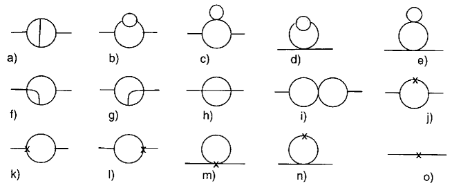
Figure 1: The topologies of the two–loop selfenergy diagrams.

In fact, the problem at hand is considerably simpler because it is essentially a one–scale problem. The Goldstone mass is zero in Landau gauge, and the only mass scale is the Higgs mass. The nonvanishing external momentum is also $s=m_{H}^{2}$ because of the on–shell renormalization scheme. This is a considerable simplification when compared with the general mass case, and indeed in ref. [15] it was possible to evaluate most diagrams involved in the calculation of the on–shell scalar selfenergies analytically. Also working in lower dimensions can make the calculation simpler. For instance, in ref. [16] the Higgs selfenergy was derived completely analytically at too–loop order as a function of the external momentum in three dimensions.

However, in more complicated cases, like for instance more external legs or arbitrary internal masses, numerical approaches seem unavoidable in realistic calculations. Details of such a general approach were described in ref. [14, 18]. Here I will only give a sketch of these techniques. The main idea is that any two–loop diagram can be expressed in terms of two basic scalar integrals ${\cal F}$ and ${\cal G}$, which are defined as follows:

$${\cal G}(m_{1},m_{2},m_{3};k^{2})\,\equiv$$ (3)

$$\int d^{n}p\,d^{n}q\,\frac{1}{(p^{2}+m_{1}^{2})^{2}\,[(q+k)^{2}+m_{2}^{2}]\,[(p+q)^{2}+m_{3}^{2}]}\,=$$

$$\pi^{4}\{\,\frac{2}{\epsilon^{2}}+\frac{1}{\epsilon}[-1+2\gamma+2\log(\pi\,m_{1}^{2})]+\frac{1}{4}+\frac{\pi^{2}}{12}$$

$$+\frac{1}{4}[-1+2\gamma+2\log(\pi\,m_{1}^{2})]^{2}-1+g(m_{1},m_{2},m_{3};k^{2})\,\}+{\cal O}(\epsilon)\;\;,$$

$${\cal F}(m_{1},m_{2},m_{3};k^{2})\,\equiv$$ (4)

$$-\int d^{n}p\,d^{n}q\,\frac{(p+q).k}{(p^{2}+m_{1}^{2})[(q+k)^{2}+m_{2}^{2}](r^{2}+m_{3}^{2})^{2}}\,=$$

$$k^{2}\pi^{4}\{\,-\frac{1}{2\epsilon}+\frac{9}{8}-\frac{1}{2}[\gamma+\log(\pi m_{1}^{2})]+f(m_{1},m_{2},m_{3};k^{2})\,\}+{\cal O}(\epsilon)\;\;.$$

The finite parts $f$ and $g$ of the scalar integrals ${\cal F}$ and ${\cal G}$ cannot be expressed in the general mass case in terms of usual functions, although it may be possible to relate them to the Lauricella function. For evaluating these functions numerically with high accuracy in an efficient way it is more convenient to use the following one–dimensional integral representations:

$$g(m_{1},m_{2},m_{3};k^{2}) = \int_{0}^{1}\,dx\,[\,Sp(\frac{1}{1-y_{1}})+Sp(\frac{1}{1-y_{2}})$$ (5)

$$+y_{1}\log\frac{y_{1}}{y_{1}-1}+y_{2}\log\frac{y_{2}}{y_{2}-1}\,]\;\;,$$

$$f(m_{1},m_{2},m_{3};k^{2}) = \int_{0}^{1}\,dx\,[\,\frac{1-\mu^{2}}{2\kappa^{2}}$$ (6)

$$-\frac{1}{2}\,y_{1}^{2}\,\log\frac{y_{1}}{y_{1}-1}-\frac{1}{2}\,y_{2}^{2}\,\log\frac{y_{2}}{y_{2}-1}\,]\;\;,$$

where the following notations were introduced:

$$y_{1,2} = \frac{1+\kappa^{2}-\mu^{2}\pm\sqrt{\Delta}}{2\kappa^{2}}$$

$$\Delta = (1+\kappa^{2}-\mu^{2})^{2}+4\kappa^{2}\mu^{2}-4i\kappa^{2}\eta\;\;,$$

$$\mu^{2} = \frac{ax+b(1-x)}{x(1-x)}$$

$$a = \frac{m_{2}^{2}}{m_{1}^{2}}\,,\;\;\;\;b\;=\;\frac{m_{3}^{2}}{m_{1}^{2}}\,,\;\;\;\;\kappa^{2}\;=\;\frac{k^{2}}{m_{1}^{2}}\;\;.$$ (7)

After continuing the integrands at complex values of the Feynman parameter $x$ and carefully inspecting the analytical properties of these functions, one is able to define an optimized integration path in terms of spline functions along which the numerical integration can be performed very efficiently. The evaluation of these functions by numerical integration with an accuracy of 8 digits takes typically about 50 ms on an HP Apollo 9000/720 workstation.

This technique was used in ref. [14, 19] to calculate the counterterms of eqns. 1 at two–loop order. A complete list of the one– and two–loop counterterms can be found for instance in ref. [18]. They agree with the results of ref. [15], which used different methods and a slightly different definition of the counterterms. Recently a similar technique was proposed for calculating a certain class of massive three–loop Feynman diagrams efficiently [17], but unfortunately at present there is no general solution which would allow one to deal in a systematic way with all possible topologies of massive three–loop diagrams.

3 Heavy Higgs decays at two–loop order

Heavy Higgs bosons mainly decay into pairs of longitudinal vector bosons and into $t\bar{t}$ pairs. At leading order, these decay widths are given by the following expressions:

$$\Gamma^{(tree)}_{H\rightarrow t\bar{t}} = \frac{3g^{2}}{32\pi}\frac{m_{H}\,m_{t}^{2}}{m_{W}^{2}}\left[1-4\frac{m_{t}^{2}}{m_{H}^{2}}\right]^{3/2}\;\;,$$

$$\Gamma^{(tree)}_{H\rightarrow W^{+}W^{-}} = \frac{g^{2}}{64\pi}\frac{m_{H}^{3}}{m_{W}^{2}}\left[1-4\frac{m_{W}^{2}}{m_{H}^{2}}\right]^{1/2}\left[1-4\frac{m_{W}^{2}}{m_{H}^{2}}+12\frac{m_{W}^{4}}{m_{H}^{4}}\right]\;\;,$$

$$\Gamma^{(tree)}_{H\rightarrow Z^{0}Z^{0}} = \frac{g^{2}}{128\pi}\frac{m_{H}^{3}}{m_{W}^{2}}\left[1-4\frac{m_{Z}^{2}}{m_{H}^{2}}\right]^{1/2}\left[1-4\frac{m_{Z}^{2}}{m_{H}^{2}}+12\frac{m_{Z}^{4}}{m_{H}^{4}}\right]\;\;.$$ (8)

For large $m_{H}$, the decays are affected by potentially large electroweak corrections of order $\lambda=(\frac{g}{4\pi}\frac{m_{H}}{m_{W}})^{2}$ at one–loop order, and of order $\lambda^{2}$ at two–loop.

The leading $m_{H}$ radiative corrections to the $H\rightarrow t\bar{t}$ decay come entirely from the counterterm contributions, and are given by a correction factor $Z_{H}/(1-\frac{\delta m_{W}^{2}}{m_{W}^{2}})$. Triangle vertex diagrams do not contribute at the order considered here because these diagrams contain additional powers of the quark mass. Therefore the leading $m_{H}$ corrections to the top decay width of the Higgs boson require only the evaluation of selfenergy diagrams. These corrections were calculated at two–loop order in ref. [19] with the methods described in the previous section, and agree with ref. [20] which uses different methods:

$$\Gamma_{H\rightarrow t\bar{t}}\,=\,\Gamma^{(tree)}_{H\rightarrow t\bar{t}}\,\times\left[1+\lambda\left(\frac{13}{8}-\frac{\pi\,\sqrt{3}}{4}\right)-\lambda^{2}\left(\,.51023\pm 2.5\cdot 10^{-4}\,\right)\right]$$ (9)

$$= \Gamma^{(tree)}_{H\rightarrow t\bar{t}}\,\left[1+.264650\,\lambda-\left(\,.51023\pm 2.5\cdot 10^{-4}\,\right)\lambda^{2}\right]\;\;.$$

For calculating the leading $m_{H}$ radiative corrections to the Higgs decay into vector bosons in a simple way, one can use the equivalence theorem and replace the external vector bosons by the corresponding Goldstone bosons. The one–loop result was derived for instance in ref. [12]. For extending this result at two–loop order, one has to calculate the diagrams shown in fig. 2. This was done in ref. [18] by using the methods described in the previous section, and the result reads:

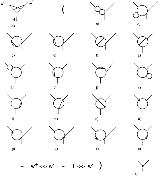
Figure 2: The topologies of the vertex diagrams which contribute to the $H\rightarrow ww$ decay at two–loop order.

$$\Gamma_{H\rightarrow W^{+}W^{-}\,,\,Z^{0}Z^{0}}\,=\,\Gamma^{(tree)}_{H\rightarrow W^{+}W^{-}\,,\,Z^{0}Z^{0}}\,\times$$ (10)

$$\left[1+\lambda\left(\frac{19}{8}+\frac{5\,\pi^{2}}{24}-\frac{3\,\sqrt{3}\,\pi}{4}\right)+\lambda^{2}\left(\,.97103\pm 8.2\cdot 10^{-4}\,\right)\right]$$

$$= \Gamma^{(tree)}_{H\rightarrow W^{+}W^{-}\,,\,Z^{0}Z^{0}}\,\left[1+.350119\,\lambda+\left(\,.97103\pm 8.2\cdot 10^{-4}\,\right)\lambda^{2}\right]\;\;.$$

This result was confirmed very recently by an independent calculation by A. Frink, B.A. Kniehl, D. Kreimer and K. Riesselmann [21], who used different methods for the evaluation of the two–loop integrals which are involved.

Of course, in eqns. 9 and 10 some incomplete subleading contributions are present in the radiative corrections. They appear if one multiplies the full tree level width, which contains for instance subleading contributions from the phase space integration and from the longitudinal vector bosons, by the radiative correction factor calculated in the leading $m_{H}$ approximation. These terms are of the same order in the coupling constant as the theoretical uncertainty related to the use of the equivalence theorem while calculating radiative corrections. It is thus not possible to decide unambiguously whether it is better to keep them or to drop them without calculating the complete subleading contributions explicitly. Numerically, this ambiguity is small and can be safely neglected.

The structure of the heavy Higgs radiative corrections to the Higgs decay width into fermions and into vector bosons is shown in fig. 3. Namely, the ratio of the decay widths including the ${\cal O}(\lambda)$ and ${\cal O}(\lambda^{2})$ radiative corrections to the tree level widths is plotted as a function of the Higgs mass. It should be remembered that the $m_{H}$ parameter is the on–shell Higgs mass as defined by the renormalization conditions of eqns. 2.

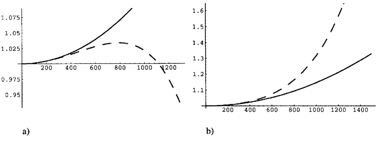
Figure 3: The magnitude of the leading $m_{H}$ radiative corrections to the $H\rightarrow t\bar{t}$ (a) and the $H\rightarrow ww$ (b) decays. The plots show the ratios of the decay widths at one–loop (solid line) and two–loop (dashed line) to the tree level decay widths as a function of the on–shell Higgs mass.

In the case of the $H\rightarrow t\bar{t}$ decay, the one–loop and the two–loop corrections have opposite signs and therefore partly compensate each other. For a Higgs mass $m_{H}\sim 1.1$ TeV the two–loop correction becomes as large as the one–loop contribution. This is an indication of the validity range of perturbation theory in the on–shell renormalization scheme. The perturbative series is at best asymptotic. Its use is motivated by the assumption that its first few terms display a reasonable convergence towards the unknown exact solution. If already the two–loop correction is as large as the one–loop one, the series appears to show no sign of convergence at all, and the validity of the perturbative approach becomes questionable. This criterion for the breakdown of the perturbation theory was used previously by van der Bij and Veltman [13] in the case of the heavy Higgs contributions to the $\rho$ parameter, and by van der Bij for the heavy Higgs corrections to the trilineal vector boson couplings [22]. They derived bounds on the Higgs mass as heavy as 3—4 TeV because of the screening of heavy Higgs effects. For the fermionic Higgs decay no screening is present, and in this case the corresponding bound is considerably lower. One also notices that the sum of the one– and two–loop radiative corrections is quite small over the whole range of validity of perturbation theory up to about 1.1 TeV. Considering also the smallness of the $t\bar{t}$ branching ratio of heavy Higgses, this makes these effects quite marginal from a phenomenological point of view.

The situation is different with the Higgs decay into vector bosons. The two–loop correction becomes larger than the one–loop contribution for a Higgs boson mass larger than $\sim 930$ GeV. The one– and two–loop corrections have the same sign and result in an enhancement of the decay width with respect to the tree level. At $m_{H}\sim 930$ GeV the one–loop correction is still rather small, at 13% level. The one–loop correction becomes numerically large only for considerably heavier Higgses, of the order of 1.3 TeV, as it was noticed in ref. [12]. Still, the perturbation theory breaks down for a Higgs mass larger than about 930 GeV in the OMS scheme. This is an interesting result which shows that a perturbative solution may be unreliable even if the one–loop radiative corrections are numerically small.

Before concluding this section, I would like to comment briefly on some speculations about the possible relevance of the perturbative result for a large Higgs mass, where the perturbative series diverges very badly. In an attempt to extend the perturbative result in this zone, one can try to construct a diagonal sequence of Padé approximants, as pointed out in ref. [19]. The hope is that this would sum up the asymptotic series, but of course there is no formal proof that this procedure converges. However, these speculations are encouraged by a relation which exists at least at leading order between the Padé approximants and the nonperturbative 1/N expansion of the $O(N)$ sigma model [23]. In the case of the fermionic Higgs decay, the [1/1] Padé approximant is a well behaved function which tends to a constant as the Higgs mass is increased. Still, in the case of the Higgs decay into vector boson pairs the [1/1] Padé approximant has a pole for a finite value of the Higgs mass, and so the relevance of the Padé approximant approach is not clear.

4 Heavy Higgs searches at hadron colliders

For $m_{H}\sim 930$ GeV, above which perturbation theory breaks down totally at least in the OMS renormalization scheme, the total one– and two–loop radiative corrections to the Higgs decay into vector bosons are quite substantial, of the order of 26%. This leaded us to consider the rôle of this type of effects in other processes of interest in view of heavy Higgs searches at future colliders. In particular, it would be interesting to investigate the relevance of radiative corrections of enhanced electroweak strength in Higgs production by gluon fusion and subsequent decay into vector bosons.

The Higgs boson can be produced by gluon fusion via a heavy quark loop. This processes is of special interest for Higgs searches at the LHC. It was studied extensively at leading order, and the next–to–leading order QCD corrections were calculated by M. Spira et al. [24]. Here we are interested in the next–to–next–to–leading order radiative corrections of enhanced electroweak strength to this process.

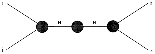
Figure 4: The structure of the radiative corrections of enhanced electroweak strength to the $t\bar{t}\rightarrow H\rightarrow zz$ scattering process. No box diagrams contribute in the order considered here because they are of higher order in the quark mass.

Before calculating the NNLO corrections to the $gg\rightarrow H\rightarrow zz$ process, it is useful to consider first the related $t\bar{t}\rightarrow H\rightarrow zz$ scattering. The structure of the leading $m_{H}$ radiative corrections to this process is shown in fig. 4. The only contributions which need to be considered are the corrections to the Higgs propagator and the corrections to the $Ht\bar{t}$ and $Hzz$ vertices. No other diagrams can contribute at the order considered here. For instance, box diagrams are of higher order in the top quark mass.

In order to calculate the radiative corrections to this scattering process consistently as an expansion in the coupling constant, one needs to pay special attention to the treatment of the Higgs resonance. The Dyson summation introduces inverse powers of the coupling constant. As a result, for deriving the complete NNLO corrections to the $t\bar{t}\rightarrow H\rightarrow zz$ process in the resonance region, one needs to include the two–loop corrections to the Yukawa coupling and to the $Hzz$ coupling, and the Higgs selfenergy up to three–loop. In fact, only the imaginary part of the three–loop Higgs selfenergy is needed at the order considered here, and this can be calculated from the two–loop Higgs decay into a pair of vector bosons and from the tree level Higgs decay into four vector bosons. The details of the calculation can be found in ref. [25]. By taking into account all relevant contributions, one obtains the full NNLO corrections to the shape of the Higgs resonance which are shown in fig. 5.

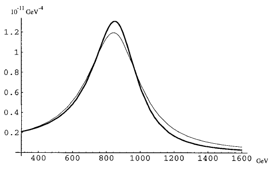
Figure 5: The effect of the NNLO corrections of enhanced electroweak strength on the shape of the Higgs resonance in the $t\bar{t}\rightarrow H\rightarrow zz$ scattering for $m_{H}=850$ GeV. The solid line is the tree level and the thin line is the NNLO result.

At this point one can calculate the corrections to the gluon fusion process. Apart from the triangular Higgs production diagram, there are also background box diagrams which contribute to the $gg\rightarrow ZZ$ process, as shown in fig. 6. The two types of diagrams behave differently as a function of the quark mass. The triangle diagram results in an effective $Hgg$ coupling in the heavy quark limit, while the box diagrams decouple. The leading $m_{H}$ correction to the triangle diagram are the same as those derived for the $t\bar{t}\rightarrow H\rightarrow zz$ scattering, and are independent of the top mass. The box diagrams can receive corrections from the rescattering of the outgoing vector bosons. These corrections are formally of order $\lambda$, but they depend on the precise ratio of the top and Higgs masses. Because the $t\bar{t}$ threshold of $\sim 360$ GeV is not negligible with respect to the Higgs mass, which will be taken of the order of 700—900 GeV, an expansion in the the top mass will probably be a not very useful approximation, and the full dependence on the top mass would need to be taken into account in these diagrams. This type of combined top–Higgs mass corrections may be numerically relevant for heavy Higgs searches at hadron colliders. Technically, their evaluation is difficult because one needs to calculate two–loop box diagrams and even three–loop vertex diagrams. Here I will consider only the universal corrections to the triangle diagram, which are independent of the top mass. This approximation is exact in the heavy top limit, when the box diagrams decouple.

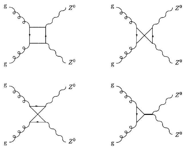
Figure 6: The leading order diagrams which contribute to the $gg\rightarrow ZZ$ process.

We have incorporated the NNLO radiative corrections of enhanced electroweak strength in a Monte Carlo simulation of the Z pair production at the LHC. The details of the calculation can be found in ref. [25]. The results of the simulation are shown in figs. 7 and 8. Comparing with the $t\bar{t}\rightarrow H\rightarrow zz$ process, one notices that the effect of the radiative corrections in gluon fusion is an enhancement of the cross section because of interference effects with the box diagrams. This enhancement is at the level of 10—20%, depending on the mass of the Higgs boson.

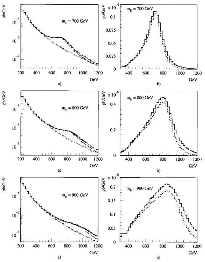
Figure 7: Invariant mass distribution of the $Z^{0}$ pairs at LHC. The processes considered are $gg\rightarrow ZZ\rightarrow 2(\mu^{+}\mu^{-})$ and $q\bar{q}\rightarrow ZZ\rightarrow 2(\mu^{+}\mu^{-})$. We consider a CM energy of 14.5 TeV, and for the outgoing muons we request $p_{T}>20$ GeV and $|y_{l}|<2.5$. The solid line is the NNLO cross section, the dashed line is the tree level cross section, and the dotted line is the background (no Higgs production diagram). a) shows the total cross section, and b) shows the Higgs signal, with the background subtracted.

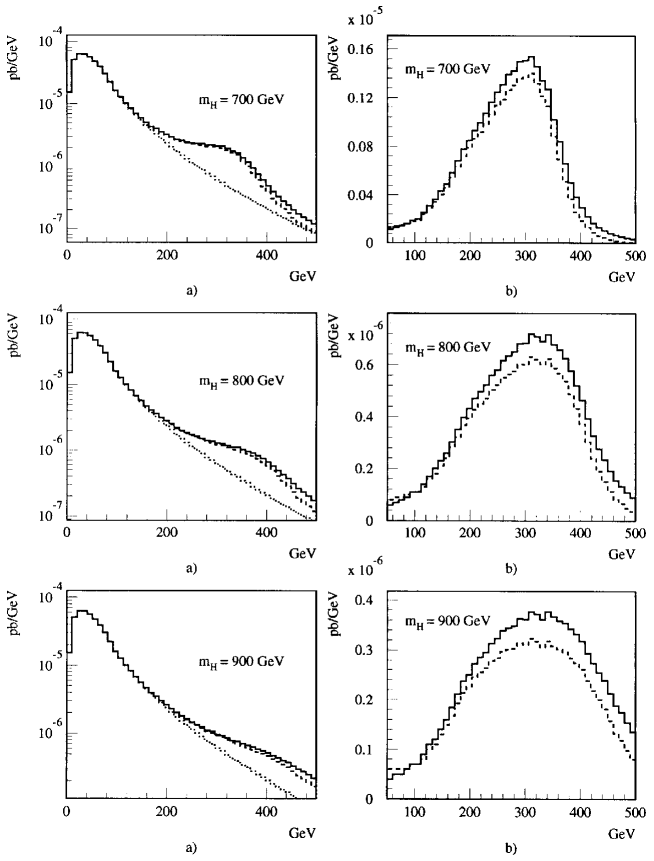
Figure 8: Transverse momentum distribution of the $Z^{0}$ bosons. Same as fig. 7.

5 Conclusions

Higher order radiative corrections of enhanced electroweak strength become increasingly important as the mass of the Higgs boson is increased. They are interesting phenomenologically in view of Higgs searches at future colliders. They also provide insight in the breakdown of perturbation theory as the Higgs selfinteraction becomes strong.

The calculations in the Higgs sector beyond one–loop level are challenging because they involve the evaluation of massive diagrams. A powerful technique is available which allows one to deal with any two–loop diagram. Similar methods were developed for a class of three–loop diagrams as well.

These techniques were used for calculating a number of processes involving the Higgs sector of the standard model at two–loop level. This allows one to set perturbative bounds on the mass of the Higgs particle, beyond which the perturbative approach is not reliable anymore.

An interesting point is that perturbation theory may cease to be reliable already for values of the coupling for which the one–loop corrections are still rather small, as it was shown explicitly in the case of the Higgs decay into vector bosons.

Finally, the analysis of the two–loop heavy Higgs effects in the Higgs boson production by gluon fusion shows that this type of effects may be numerically important for heavy Higgs searches at the LHC.

An interesting point which I did not discuss is the longitudinal vector boson scattering. This process shows promise of providing insight in the spontaneous electroweak symmetry breaking mechanism, and becomes important as a source of Higgs bosons at hadron colliders for $m_{H}\sim 1$ TeV. This process was studied at one–loop order in ref. [26, 27]. At two–loop level only a calculation in the high energy limit exists, where the Feynman diagrams which are involved are simpler [15]. A complete two–loop analysis would be difficult because it involves the calculation of two–loop massive box diagrams. This is an interesting problem which deserves further investigation.

Acknowledgement

I would like to thank the theory department of the Brookhaven National Laboratory, where this paper was written, for hospitality, and the U.S. Department of Energy (DOE) for support. This work was supported by the Deutsche Forschungsgemeinschaft (DFG).

References

- [1] S. Dittmaier, D. Schildknecht, G. Weiglein, BI-TP-96-14 (1996), hep-ph/9605268.
- [2] M. Veltman, Phys. Lett. B139 (1984) 307.
- [3] M.B. Einhorn, Nucl. Phys. B246 (1984) 75.
- [4] R.G. Root, Phys. Rev. D10 (1974) 3322.
- [5] J.P. Nunes, H.J. Schnitzer, Int. J. Mod. Phys. A10 (1995) 719.
- [6] A. Hasenfratz, K. Jansen, J. Jersak, C.B. Lang, T. Neuhaus, H. Yoneyama, Nucl. Phys. B317 (1989) 81.
- [7] U.M. Heller, H. Neuberger, P. Vranas, Phys. Lett. B283 (1992) 335.
- [8] D.B. Stephenson, A. Thornton, Phys. Lett. B212 (1988) 479.
- [9] D.J.E. Callaway, Phys. Rept. 167 (1988) 241.
- [10] these Proceedings, the contributions by S. Larin, T. van Ritbergen, A. Kataev.
- [11] F.A. Berends, M. Buza, M. Böhm and R. Scharf, Z. Phys. C63 (1994) 227.
- [12] W.J. Marciano and S.S.D. Willenbrock, Phys. Rev. D37 (1988) 2509.
- [13] J.J. van der Bij and M. Veltman, Nucl. Phys. B231 (1984) 205.
- [14] A. Ghinculov and J.J. van der Bij, Nucl. Phys. B436 (1995) 30.
- [15] P.N. Maher, L. Durand, K. Riesselmann, Phys. Rev. D48 (1993) 1061; (E) D52 (1995) 553.
- [16] A.K. Rajantie, HU-TFT-96-22 (1996), hep-ph/9606216.
- [17] A. Ghinculov, Freiburg-THEP-96-6 (1996), hep-ph/9604333.
- [18] A. Ghinculov, Nucl. Phys. B455 (1995) 21.
- [19] A. Ghinculov, Phys. Lett. B337 (1994) 137; (E) B346 (1995) 426.
- [20] L. Durand, B.A. Kniehl and K. Riesselmann, Phys. Rev. D51 (1995) 5007; Phys. Rev. Lett. 72 (1994) 2534; (E) Phys. Rev. Lett. 74 (1995) 1699.
- [21] A. Frink, B.A. Kniehl, D. Kreimer, K. Riesselmann, LMU-04-96 (1996), hep-ph/9606310.
- [22] J.J. van der Bij, Nucl. Phys. B255 (1985) 648.
- [23] S. Willenbrock, Phys. Rev. D43 (1991) 1710.
- [24] M. Spira, A. Djouadi, D. Graudenz, P.M. Zerwas, Nucl. Phys. B453 (1995) 17.
- [25] A. Ghinculov and J.J. van der Bij, Freiburg-THEP-95-25 (1995), hep-ph/9511414.
- [26] S. Dawson, S. Willenbrock, Phys. Rev. D40 (1989) 2880.
- [27] M.J.G. Veltman and F.J. Yndurain, Nucl. Phys. B325 (1989) 1.