CERN-TH-96/188

TAUP-2355-96

LBNL-39135

hep-ph/9607404

Renormalization-Scheme Dependence of Padé Summation in QCD
John Ellis
Theoretical Physics Division, CERN, CH-1211 Geneva 23, Switzerland
e-mail: john.ellis@cern.ch
Einan Gardi and Marek Karliner
School of Physics and Astronomy
Raymond and Beverly Sackler Faculty of Exact Sciences
Tel-Aviv University, 69978 Tel-Aviv, Israel
e-mail: gardi@post.tau.ac.il, marek@vm.tau.ac.il
and
Mark A. Samuel
Department of Physics, Oklahoma State University,
Stillwater, Oklahoma 74078, USA
e-mail: physmas@mvs.ucc.okstate.edu
Abstract

We study the renormalization-scheme (RS) dependence of Padé Approximants (PA’s), and compare them with the Principle of Minimal Sensitivity (PMS) and the Effective Charge (ECH) approaches. Although the formulae provided by the PA, PMS and ECH predictions for higher-order terms in a QCD perturbation expansion differ in general, their predictions can be very close numerically for a wide range of renormalization schemes. Using the Bjorken sum rule as a test case, we find that Padé Summation (PS) reduces drastically the RS dependence of the Bjorken effective charge. We use these results to estimate the theoretical error due to the choice of RS in the extraction of $\alpha_{s}$ from the Bjorken sum rule, and use the available data at $Q^{2}=3$ GeV² to estimate $\alpha_{s}(M_{Z})=0.117^{+0.004}_{-0.007}\,\pm 0.002$, where the first error is experimental, and the second is theoretical.

CERN-TH-96/188

July 1996

1 Introduction

Padé approximants (PA’s) have proven to be useful in many physics applications, including condensed-matter problems and quantum field theory [1]. PA’s may be used either to predict the next term in some perturbative series, called a Padé Approximant prediction (PAP), or to estimate the sum of the entire series, called Padé Summation (PS). The underlying reasons for the successes of these different applications have not always been apparent. Admittedly, rational functions are very flexible, and hence a priori well suited to approximate other unknown functions, but some of the PA successes seem almost ‘magical’. Obtaining a deeper understanding of these successes is not only desirable in itself, but may give us deeper understanding also of the underlying physics. Among the areas in which PA’s have had remarkable successes has been perturbative QCD [2, 3] where PA’s applied to low-order perturbative series have been shown to ‘postdict’ accurately known higher-order terms, and also used to make estimates of even higher-order unknown terms that agree with independent predictions based on the Principle of Minimal Sensitivity (PMS) [4] and Effective Charge (ECH) [5] techniques. Of particular interest to us has been the perturbative QCD series for the Bjorken sum rule for three quark flavors [6, 7, 8] which has served us previously [3] as a test case. For this series, the [0/1] PAP for the third-order coefficient in the $\overline{\hbox{MS}}\,$ prescription is $12.8$, to be compared with the PMS estimate of $20.0$, the ECH estimate of $19.2$, and the exact value [8] of $20.21$ . This lowest-order PAP is pointing in the right direction, which is the best one could hope at this level. Going to the next order, the [1/1] and [0/2] PAP’s for the fourth-order Bjorken sum rule coefficient are $114$ and $99$ respectively, whilst the PMS/ECH prediction is $130$ [10]. These values are quite similar, and we have provided [3] a prescription for systematic improvement of these PAP’s which brings them even closer to the PMS/ECH prediction. Should the previous agreement of PAP’s with the PMS/ECH and exact calculations here and elsewhere, and the agreement of these new predictions, be regarded as fortuitous, or is there some deeper reason why PAP’s and PS’s should be believed also in the QCD context?

In recent papers [2, 3], we have tried to cast some light on these ‘magical’ successes. In particular, we have proven that certain conditions on the ratios of consecutive terms in a series are mathematically sufficient to guarantee rapid convergence of successive PAP’s, and we have observed that these conditions are satisfied by asymptotic series dominated by one or a finite number of renormalon poles. This is believed to be the case for many QCD perturbation series, such as that for the Bjorken sum rule [9], which we have used as a testing ground and showcase. We have also shown that PA’s yield a renormalization-scale dependence which is much less than that of the corresponding perturbative series, even when the latter is supplemented by an ECH estimate of the next, uncalculated term. Since the full QCD expression for any physical quantity such as the Bjorken sum rule must be renormalization-scale independent, this is valuable circumstantial evidence that the PA’s are indeed converging towards the correct physical result. However, the strength of this evidence is significantly reduced by the fact that the scale dependence has been studied only within one specific renormalization scheme, namely $\overline{\hbox{MS}}\,$, making it difficult to assess the numerical accuracy of the PA prediction.

The purpose of this paper is to understand better the renormalization-scheme dependence of PA’s in perturbative QCD, again taking the Bjorken sum rule as our test case. On the way to this goal, we also examine more closely the relations between PAP’s and the PMS and ECH techniques for estimating higher-order perturbative coefficients in QCD, and examine the extent to which PS’s should and do agree with PMS and ECH estimates of the ‘sums’ of perturbative series in QCD. We also examine the extent to which the Cancelation Index (CI) criterion of Ref. [11] provides a reliable guide to the comparative accuracies of partial calculations in different renormalization schemes.

The PMS and ECH formulae used to predict the next term in any QCD perturbative series do not in general coincide, and we show below that the PA prediction (PAP) for the next term is in general different again. However, in a wide range of RS’s their predictions can be quite close numerically, as we discuss later.

Using the Bjorken sum rule as an example, we exhibit a map of its two-parameter renormalization-scheme dependence at the next-to-next-to-leading order (NNLO) level, situating on this map the PMS and ECH scheme choices. We then exhibit the corresponding map for the [0/2] PA, which we find to be much less sensitive to the choice of renormalization scheme. We also demonstrate that the CI criterion of Ref. [11] selects efficiently the region of renormalization-scheme space where the scheme-dependence is minimized. In addition, we compare the PMS/ECH and [0/2] PA predictions for the fourth-order term in the Bjorken sum rule series, finding remarkable agreement.

Finally, as an application of this analysis, we revisit the extraction [3] of $\alpha_{s}$ from experimental data on the Bjorken sum rule at $Q^{2}=3$ GeV². Our analysis enables us to assign a systematic error to the choice of renormalization scheme, which is small compared with the current experimental error. The present data yield

$$\alpha_{s}(M_{Z})\,=\,0.117\,\,{}^{+0.004}_{-0.007}\,\hbox{(exp.)}\,\,{}^{+0.002}_{-0.002}\,\hbox{(th.)}$$ (1)

which could in the future become a highly competitive determination of $\alpha_{s}(M_{Z})$, if the present experimental error could be halved. The systematic error associated with the choice of renormalization scale would still not be dominant at this level.

2 Comparing PMS, ECH and Padé Predictions to NNLO

We start by recalling the essential physical ideas of the PMS [4] and ECH [5] approaches. The PMS method is based on choosing the RS that minimises the RS dependence in a given order of perturbation theory, whereas, in the ECH method, one chooses a natural RS to describe the observable, namely one in which all the non-leading corrections are exactly zero. To see how these work and differ in practice, we look at the application of PMS and ECH to the perturbative series for a generic QCD observable, calculated at NLO and NNLO in some RS. At the NLO level, the choice of RS involves just the choice of renormalization scale $\mu$, whereas a second parameter enters at the NNLO level, as we discuss in more detail later. For convenience, instead of $\mu$, we use $\tau$, defined by

$$\tau=b\ln\left(\frac{\mu}{\Lambda}\right)\,,\qquad\qquad b=\frac{33-2N_{f}}{6}\,.$$ (2)

At NLO any observable $\hat{O}$ can be written as:

$$\hat{O}=a(\tau)[1+r_{1}(\tau)a(\tau)]$$ (3)

where $a(\tau)\equiv{\alpha_{s}(\tau)}/{\pi}$ satisfies the renormalization-group equation at NLO:

$$\frac{\partial a}{\partial\tau}=\frac{1}{b}\mu\frac{\partial a}{\partial\mu}=-a^{2}\left[1+ca\right]\,,\qquad\qquad\qquad c=\frac{153-19N_{f}}{2(33-2N_{f})}\,.$$ (4)

which has the solution:

$$\tau=\frac{1}{a}+c\ln\left(\frac{ca}{1+ca}\right)$$ (5)

In the PMS method [4] one chooses an ‘optimal RS’ which minimises the RS dependence at a given order. The corresponding parameters are denoted by: $\overline{\tau}$,$\overline{a}$, $\overline{r_{1}}$. In order to find the PMS RS, one differentiates (3) with respect to $\tau$, substituting $\partial a/\partial\tau$ from (4), yielding

$$\frac{\partial\hat{O}}{\partial\tau}=a^{2}\left(-1+\frac{\partial r_{1}}{\partial\tau}\right)-a^{3}(2r_{1}ca+c+2r_{1})$$ (6)

Clearly, at NLO the ${\cal O}(a^{2})$ RS dependence of any observable must vanish, and therefore ${\partial r_{1}}/{\partial\tau}=1$. Thus one identifies the RG invariant $\rho_{1}$:

$$\rho_{1}=\tau-r_{1}$$ (7)

which enables us to calculate $r_{1}(\tau)$ in any RS from an initial $r_{1}$ that was calculated in perturbation theory in some initial RS. Equating ${\partial\hat{O}}/{\partial\tau}$ in (6) to zero, one finds that in the PMS RS:

$$\overline{r_{1}}=-\,\frac{c}{2(1+c\overline{a})}$$ (8)

and therefore, using (7), (5), and (8) one can write an equation for $\overline{a}$:

$$\rho_{1}=\frac{c}{2(1+c\overline{a})}+\frac{1}{\overline{a}}+c\ln\left(\frac{c\overline{a}}{1+c\overline{a}}\right)$$ (9)

This equation cannot be solved analytically, but it can directly be solved numerically. Finally, one uses (8) to write the observable in the PMS RS:

$$\hat{O}_{PMS}=\overline{a}\frac{2+c\overline{a}}{2(1+c\overline{a})}$$ (10)

Substituting $\overline{a}$ as a power series in the original $a$, we obtain a ratio of two polynomials in $a$, that is – a structure similar to Padé-Summation! With the resemblance comes the difference: The PMS result depends not only on the lower order coefficients of the observable we are dealing with, but also on the coefficients of the $\beta$ function (this is also the case in the BLM method).

In the ECH method [5], the preferred RS is the one is which the perturbative expansion (like eq (3) ) reduces to a leading term, that is:

$$\hat{O}_{ECH}=a^{*}.$$ (11)

We can find this RS by substituting $r_{1}=0$ in (7). Using (5) we can write the following equation for $a^{*}$:

$$\rho_{1}=\frac{1}{a^{*}}+c\ln\left(\frac{ca^{*}}{1+ca^{*}}\right)$$ (12)

As in the PMS case, this equation can only be solved numerically. In this case, we do not find any resemblance to the Padé structure.

At NNLO $a\equiv\alpha_{s}(\tau)/\pi$ satisfies the RG equation:

$$\frac{\partial a}{\partial\tau}=\frac{1}{b}\mu\frac{\partial a}{\partial\mu}=-a^{2}\left[1+ca+c_{2}a^{2}\right]\equiv\frac{\beta{(a)}}{b}$$ (13)

which has the formal solution:

$$\tau=\frac{1}{a}+c\,\ln\left(\frac{ca}{1+ca}\right)+c_{2}\int_{0}^{a}\frac{dx}{(1+cx)\,(1+cx+c_{2}x^{2})}$$ (14)

The two independent parameters specifying the RS may be chosen to be $a$ and $c_{2}$ or $\tau$ and $c_{2}$. For our present purposes, it is more convenient to use $\tau$ and $c_{2}$. A generic QCD observable at the NNLO may then be written in the form:

$$\hat{O}=a\,\left[\,1\,+\,r_{1}(\tau,c_{2})\,a\,+\,r_{2}(\tau,c_{2})\,a^{2}\,\right]\,,$$ (15)

where $a\equiv a(\tau,c_{2})$. To derive the second-order PMS formulae, we first differentiate the observable (15) with respect to both $\tau$ and $c_{2}$:

$$\frac{\partial\hat{O}}{\partial\tau}=\frac{\partial a}{\partial\tau}\left(1+2r_{1}a+3r_{2}a^{2}\right)+a^{2}\,\frac{\partial r_{1}}{\partial\tau}+a^{3}\,\frac{\partial r_{2}}{\partial\tau}$$ (16)

$$\frac{\partial\hat{O}}{\partial c_{2}}=\frac{\partial a}{\partial c_{2}}\left(1+2r_{1}a+3r_{2}a^{2}\right)+a^{2}\,\frac{\partial r_{1}}{\partial c_{2}}+a^{3}\,\frac{\partial r_{2}}{\partial c_{2}}$$ (17)

Using next the NNLO renormalization-group equation (13), we can find ${\partial a/\partial c_{2}}$ as a function of $a$, $c$ and $c_{2}$ and substitute ${\partial a/\partial\tau}$ and ${\partial a/\partial c_{2}}$ for the appropriate power series in $a$ in equations (16) and (17). Demanding that ${\partial\hat{O}}/{\partial\tau}$ and ${\partial\hat{O}}/{\partial c_{2}}$ be of order $O(a^{4})$, we find two renormalization-group-invariant quantities:

$$\rho_{1}=\tau-r_{1}$$ (18)

which appears already in a NLO analysis, and

$$\rho_{2}=r_{2}+c_{2}-r_{1}^{2}-r_{1}c$$ (19)

Using these two invariants, we can calculate $r_{1}(\tau,c_{2})$ and $r_{2}(\tau,c_{2})$ in any RS, as a function of the values of $r_{1}$ and $r_{2}$ calculated in perturbation theory in any initial RS. We will use (18) and (19) extensively later in this work.

The two equations that determine the PMS RS can now be found by equating (16) and (17) to zero. These equations cannot be solved analytically, but one may solve them graphically to locate the PMS RS, by plotting the NNLO observable as a function of the RS parameters $a$ and $c_{2}$, and identifying a local extremum or saddle point, which corresponds to both (16) and (17) being zero.

The ECH RS is specified at third order by the conditions $r_{1}=r_{2}=0$, which we must substitute into equations (18) and (19). The results are:

$$\tau_{\,ECH}=\rho_{1}$$ (20)

and,

$$c_{2\,ECH}=\rho_{2}$$ (21)

Substituting the above in (14), we obtain an equation for $a^{*}$, which is just the observable calculated in the ECH scheme, $\hat{O}_{ECH}=a^{*}$:

$$\rho_{1}=\frac{1}{a^{*}}+c\ln\left(\frac{ca^{*}}{1+ca^{*}}\right)+\rho_{2}\int_{0}^{a^{*}}\frac{dx}{(1+cx)(1+cx+\rho_{2}x^{2})}$$ (22)

As in the PMS case, this ECH equation cannot be solved analytically.

Since there are no closed analytical formulae for the third-order PMS and ECH results, we cannot compare them directly to the PS method. We do note, however, that the PMS and ECH expressions contain in general singularities in the coupling plane, as do Padé approximants. Still, the PMS singularities are not necessarily discrete poles, and thus the PMS and ECH singularity structure may differ from that of the PS. Here we do not address this interesting issue further, focusing instead on comparing Padé with PMS/ECH. The comparison is done by looking both at their predictions of for the next term in the perturbative series, and at their results for the overall ‘summation’ of the series.

As a warm-up exercise, we consider the comparison at NLO, where we start with (3) and predict $r_{2}$ by the different methods. To this order, the [0/1] PAP is equivalent to the assumption that the series is a geometrical one, so that:

$$r_{2}^{PAP}=r_{1}^{2}$$ (23)

On the other hand, it follows from the above higher-order analysis that the PMS prediction is [4]:

$$r_{2}^{PMS}=\left(r_{1}+\frac{1}{2}c\right)^{2}$$ (24)

whilst the ECH result is [5]:

$$r_{2}^{ECH}=r_{1}^{2}+r_{1}c$$ (25)

We observe that, if $r_{1}$ is much larger than $c$, then the three methods will give similar results. However, $c$ does not depend on the RS, while $r_{1}$ does. This means that there are schemes in which the PAP, PMS and ECH would be close, and others (which may be just as legitimate) in which they would not agree. It is however clear from equations (24) and (25) that the schemes in which there is a good agreement between the PMS and ECH predictions are exactly those schemes in which the PAP prediction (23) agrees with both of them.

In order to study this comparison between Padé and PMS further, we go to third order, where a generic observable may be written as in (15). The PAP predictions for the 4-th coefficient ($r_{3}$) are:

$$r_{3}^{[1/1]\,PAP}=\frac{r_{2}^{2}}{r_{1}}$$ (26)

$$r_{3}^{[0/2]\,PAP}=-r_{1}^{3}+2r_{1}r_{2}$$ (27)

whilst the PMS and ECH predictions coincide exactly [10]:

$$r_{3}^{PMS}=r_{3}^{ECH}=r_{1}\left(3r_{2}-2r_{1}^{2}+c_{2}-\frac{cr_{1}}{2}\right)$$ (28)

We see from the above that there is no simple relation between the formulae for the PAP and the PMS/ECH predictions.

At NLO, eqs. (23), (24), (25), they differ only by terms that depend on a higher-order coefficient in the QCD $\beta$ function. However, there are further differences at NNLO, eqs. (26), (27), (28). There are, nevertheless, a couple of extreme cases in which the predictions of the different methods for $r_{2}$ and for $r_{3}$ approach each other. One such case is provided by RS’s in which all the non-leading corrections are small, or even zero as in the ECH RS. The prediction for the next term is then small in all approaches, as intuitively expected. The other extreme is when the non-leading corrections are much larger than the corresponding coefficients of the $\beta$ function ($r_{i}\gg c_{i}$). In this case the NLO prediction is $r_{2}^{est}\sim r_{1}^{2}$ in any method, and the NNLO prediction is $r_{3}^{est}\sim r_{1}^{3}$ in any method, provided that the $r_{2}$ coefficient is indeed close to the NLO prediction, i.e., $r_{2}\sim r_{1}^{2}$. It cannot be guaranteed, however, that either of these conditions holds for a generic observable in a generic RS. Therefore, the formulae for the next term derived in the different methods do not generally coincide. Still, a good numerical agreement between the predictions is possible in a generic RS, and this is indeed the case in the example we discuss later.

The principal conclusions of this analysis are:

a)   There is no general agreement, nor simple relation between the PMS or the ECH methods and the Padé method. One major reason for this is that, in contrast to the PA’s, the PMS and ECH predictions depend on the coefficients of the $\beta$ function, and not only on the coefficients of the observable under consideration.

b)   PA’s differ from conventional perturbation series by having distinctive singularities in the coupling plane. While some singularities may be expected in QCD, they are not necessarily of the Padé form. Singularities in the coupling plane appear also in the PMS and ECH formulations, e.g., the second-order PMS result is just a rational polynomial. Higher-order PMS and ECH results cannot be calculated analytically, but singularities in the coupling plane are expected there as well. However, there is at present no indication that the singularity structure will resemble that of the PA.

c)   Since the PA method is totally independent of the PMS and ECH methods, we believe that good numerical agreement between their predictions should be considered as strong evidence that both sets of predictions are correct.

As a test case for the application of the PMS, ECH and PA approaches, we study in the following sections the Bjorken Sum Rule for three quark flavours. Our conclusions can later be checked using other QCD observables.

3 Renormalization-Scheme Dependence in the Bjorken Sum Rule

We now proceed to a detailed discussion of renormalization-scheme (RS) dependence in one of the cases where an exact NNLO perturbative calculation in available, namely the effective charge in the Bjorken sum rule [6, 7, 8]:

$$a^{*}_{Bj}=a\,+\,3.58\,a^{2}\,+\,20.22\,a^{3}\,+\,\cdots$$ (29)

in the $\overline{\hbox{MS}}\,$ scheme with $\mu=Q$ and 3 flavours assumed. It is a simple matter to convert (29) to an arbitrary renormalization scheme, using the two RG invariants of eq. (18) and (19).

We note at the outset of our analysis that the PMS and ECH prescriptions are both based explicitly on the renormalization group, and aim directly at the choice of an optimal RS. The BLM approach [12] is also based on the renormalization group, and can be regarded as a way of choosing systematically renormalization scales appropriate for each order in perturbation theory. As we discuss in [13], the BLM approach is close to PMS and ECH, both in its nature and its results. On the other hand, Padé approximants are formulated independently of the renormalization group in any RS, and we have demonstrated explicitly in the previous section that they are not related to PMS and ECH in any obvious way. Hence, there is no a priori reason to expect the Padé method to reduce the RS dependence. In fact it does, as we shall see later, and we believe that this observation bolsters the utility of Padé approximants in QCD applications.

We first compute the Bjorken effective charge $a^{*}_{Bj}$ as a function of the two NNLO parameters $a$ and $c_{2}$ discussed in the previous section. Experimental measurements of the Bjorken sum rule are currently made in a range of $Q^{2}$ where one believes 3 quark flavours to be active, as assumed in (29). In principle, as $\mu$ is varied, one may cross the charm threshold, and so one should modify and match formulae (13) and (29) of effective theories at the $N_{f}=4$ threshold. Since this issue is only a technical complication, we choose to avoid it for the purposes of this discussion by calculating the Bjorken effective charge at $Q^{2}=20$ GeV², corresponding to $a=0.07$ in the $\overline{\hbox{MS}}\,$ prescription with $\mu=Q$, and fixing $N_{f}=3$, whatever the value of $\mu$. This analysis is sufficient to establish a “proof of concept”, and we return later to a discussion of the more experimentally relevant case of lower $Q^{2}$. Fig. 1 displays contours of the Bjorken effective charge $a^{*}_{Bj}$, differing in height by $\Delta\hbox{$a^{*}_{Bj}$}=0.002$, where we note the following features:

a)   There is a flat region around $a=0.1$, where the RS dependence is very weak.

b)   The value of the Bjorken effective charge in the $\overline{\hbox{MS}}\,$ RS ($a=0.07$, $c_{2}=4.471$, denoted by a circle) is

$$\hbox{$a^{*}_{Bj}$}(\hbox{$\overline{\hbox{{\footnotesize MS}}}\,$})=0.09449$$ (30)

We note that the $\overline{\hbox{MS}}\,$ RS does not lie in the flat region mentioned above. Therefore the RS dependence, particularly the renormalization scale dependence, is relatively high in the $\overline{\hbox{MS}}\,$ RS.

c)   Within the flat region mentioned in a), there is a saddle point at $a=0.1005$, $c_{2}=8.7$, which corresponds to the PMS RS . The value of the Bjorken effective charge in the PMS RS is

$$\hbox{$a^{*}_{Bj}$}(\hbox{\footnotesize PMS})=0.10033$$ (31)

which deviates by about $6\%$ from the $\overline{\hbox{MS}}\,$ result. This deviation is an example of the RS dependence in this case.

d)   Another point which lies in the flat region mentioned in a) is the ECH RS at $a=0.10038$, $c_{2}=5.476$. The value of the Bjorken effective charge in the ECH method is therefore

$$\hbox{$a^{*}_{Bj}$}(\hbox{\footnotesize ECH})=0.10038$$ (32)

which is very close to the PMS result of (31).

e)   When using a RS with a very low coupling-constant ($a\mathrel{\mathchoice{\vbox{\offinterlineskip\halign{$\m@th\displaystyle\hfil#\hfil$\cr<\crcr\sim\crcr} }}{\vbox{\offinterlineskip\halign{$\m@th\textstyle\hfil#\hfil$\cr<\crcr\sim\crcr} }}{\vbox{\offinterlineskip\halign{$\m@th\scriptstyle\hfil#\hfil$\cr<\crcr\sim\crcr} }}{\vbox{\offinterlineskip\halign{$\m@th\scriptscriptstyle\hfil#\hfil$\cr<\crcr\sim\crcr} }}}0.04$, for example) or a very high coupling-constant ($a\mathrel{\mathchoice{\vbox{\offinterlineskip\halign{$\m@th\displaystyle\hfil#\hfil$\cr>\crcr\sim\crcr} }}{\vbox{\offinterlineskip\halign{$\m@th\textstyle\hfil#\hfil$\cr>\crcr\sim\crcr} }}{\vbox{\offinterlineskip\halign{$\m@th\scriptstyle\hfil#\hfil$\cr>\crcr\sim\crcr} }}{\vbox{\offinterlineskip\halign{$\m@th\scriptscriptstyle\hfil#\hfil$\cr>\crcr\sim\crcr} }}}0.16$, for example) we obtain a value of $a^{*}_{Bj}$ which is totally inconsistent with the $\overline{\hbox{MS}}\,$, PMS and ECH results, and which is also strongly dependent on the specific choice of the parameters $a$ and $c_{2}$. This strong deviation from the results of the ECH and PMS RS’s is related to the existence of large non-leading corrections in the perturbative expansion for the Bjorken Sum Rule in these RS’s. Therefore, we look for a consistent way of excluding these RS’s, or – even better – a consistent way of using them and still getting reasonable results. We will now show that both aims are achievable, the first by the use of the Cancellation Index criterion advocated in Ref. [11], which is discussed in the following section, and the second by the use of PS, as shown in section 5.

4 The Cancellation Index Criterion

In view of the NNLO RS dependence on $a$ and $c_{2}$ displayed in Fig. 1, it is desirable to find a criterion which selects a region in the $(a,\,c_{2})$ plane that contains “well-behaved” RS’s for which higher-order corrections are not expected to be large. One can then examine the performance of techniques for improving the perturbative series (such as the Padé method) in a compact domain of the $(a,\,c_{2})$ plane. Looking at the RS dependence over this domain may then provide a legitimate estimate of the observable ($a^{*}_{Bj}$ in our test case) and of the RS uncertainty in this estimate.

Here we use the criterion proposed in Ref. [11], namely that a “well-behaved” RS is one for which the degree of cancellation between the different terms in the second NNLO renormalization-group invariant $\rho_{2}=r_{2}+c_{2}-r_{1}^{2}-cr_{1}$ (19) is small. The degree of cancellation is measured by the Cancellation Index:

$${\cal C}=\frac{|r_{2}|+|c_{2}|+r_{1}^{2}+c|r_{1}|}{r_{2}+c_{2}-r_{1}^{2}-cr_{1}}$$ (33)

and contours of ${\cal C}$ for the Bjorken effective charge $a^{*}_{Bj}$ are also plotted in Fig. 1 . We exhibit the contours ${\cal C}=2,3,4,5$: contours of higher values of ${\cal C}$ become closer together as ${\cal C}$ increase.

We observe that these contours of ${\cal C}$ are indeed centered around the flat region of small RS dependence to which we drew attention previously. Indeed, the ECH RS is the only one for which ${\cal C}=1$. The PMS RS also has a low value ${\cal C}=2.18$, whereas ${\cal C}\mathrel{\mathchoice{\vbox{\offinterlineskip\halign{$\m@th\displaystyle\hfil#\hfil$\cr>\crcr\sim\crcr} }}{\vbox{\offinterlineskip\halign{$\m@th\textstyle\hfil#\hfil$\cr>\crcr\sim\crcr} }}{\vbox{\offinterlineskip\halign{$\m@th\scriptstyle\hfil#\hfil$\cr>\crcr\sim\crcr} }}{\vbox{\offinterlineskip\halign{$\m@th\scriptscriptstyle\hfil#\hfil$\cr>\crcr\sim\crcr} }}}7$ for the $\overline{\hbox{MS}}\,$ RS, as was already mentioned in [11].

In order to study the RS dependence we restrict our attention to the domain defined by ${\cal C}\leq{\cal C}_{0}$. ${\cal C}_{0}$ should be chosen such that the PMS RS, where the local RS dependence vanishes is well within the selected domain, but yet, not too large, so that all the RS included in the domain would be trustable, having a small enough local RS dependence. For the purposes of the subsequent discussion, we shall choose ${\cal C}_{0}=4$  which answers the above requirements. While other reasonable values of ${\cal C}_{0}$ and other criteria for choosing restricted domains in the RS parameter space may be used just as well, our principle conclusions would remain the same.

Within the ${\cal C}\leq 4$ domain, we find

$$0.087\,\leq\,\hbox{$a^{*}_{Bj}$}\,\leq\,0.109$$ (34)

which is our best estimate of the likely RS ambiguity in $a^{*}_{Bj}$, in the absence of the improvement that the Padé method provides in the next section.

5 Padé Summation of the Bjorken Series

We now apply the Padé method to the perturbative QCD series for the Bjorken effective charge (29), and explore its effect on the RS dependence. As already mentioned in the Introduction, one may use Padé approximants either to predict the next term in the series (PAP) or to sum the entire series (PS), in the sense [3] of calculating the Cauchy principal value of an asymptotic series with one or more infrared renormalons, as is believed to be the case for the Bjorken series.

A priori, one may evaluate either the [0/2] PS or the [1/1] PS of the Bjorken series. In this section we evaluate both PS’s of the Bjorken series in the $(a,\,c_{2})$ plane introduced earlier, and compare their RS dependences with that of the naïve series shown in Fig. 1.

Fig. 2 displays contours of $a^{*}_{Bj}$ evaluated using the [0/2] PS, with the same steps $\Delta\hbox{$a^{*}_{Bj}$}=0.002$ as in Fig. 1 . We see immediately that the contours in Fig. 2 are much sparser than those in Fig. 1, and hence that the [0/2] PS depends much less on the RS than does the naïve partial sum. To put this comparison on a quantitive basis, we evaluate the RS dependence of $a^{*}_{Bj}$( [0/2] PS ) in the ${\cal C}\leq 4$ domain of the $(a,\,c_{2})$ plane:

$$0.0986\,\leq\,\hbox{$a^{*}_{Bj}$}(\,[0/2]\,PS\,)\,\leq\,0.1011$$ (35)

We see that the RS dependence of the [0/2] PS is an order of magnitude less than that of the naïve partial sum (29).

This is not true, however, for the [1/1] PS shown in Fig. 3, whose RS-dependence is much larger to that of the naïve partial sum:

$$-0.14\,\mathrel{\mathchoice{\vbox{\offinterlineskip\halign{$\m@th\displaystyle\hfil#\hfil$\cr<\crcr\sim\crcr} }}{\vbox{\offinterlineskip\halign{$\m@th\textstyle\hfil#\hfil$\cr<\crcr\sim\crcr} }}{\vbox{\offinterlineskip\halign{$\m@th\scriptstyle\hfil#\hfil$\cr<\crcr\sim\crcr} }}{\vbox{\offinterlineskip\halign{$\m@th\scriptscriptstyle\hfil#\hfil$\cr<\crcr\sim\crcr} }}}\,\hbox{$a^{*}_{Bj}$}(\,[1/1]\,PS\,)\,\mathrel{\mathchoice{\vbox{\offinterlineskip\halign{$\m@th\displaystyle\hfil#\hfil$\cr<\crcr\sim\crcr} }}{\vbox{\offinterlineskip\halign{$\m@th\textstyle\hfil#\hfil$\cr<\crcr\sim\crcr} }}{\vbox{\offinterlineskip\halign{$\m@th\scriptstyle\hfil#\hfil$\cr<\crcr\sim\crcr} }}{\vbox{\offinterlineskip\halign{$\m@th\scriptscriptstyle\hfil#\hfil$\cr<\crcr\sim\crcr} }}}\,0.14$$ (36)

The extremes of this large range are due to specific RS’s for which the [1/1] PS is particularly deviant. Most RS’s fall within a much narrower range. However, this analysis points up the fact that the [1/1] PS is much less well-behaved than the [0/2] PS (35).

A persistent problem in the application of Padé methods is how to choose the one which is the most accurate. Various empirical and analytic results give some indications, but there is no unambiguous general prescription for the choice. In the case of the Bjorken series at the NNLO level, the amount of RS dependence provides a clear physical criterion, which selects unambiguously the [0/2] PS. The reduced RS dependence (35) of the $a^{*}_{Bj}$( [0/2] PS ) hints that this determination of $a^{*}_{Bj}$ may be correct within its errors. One might worry that the PS for different RS are converging to the wrong common result. However, encouragement is provided by the comparison between the PMS, ECH and PS results (31), (32) and (35), where we see that they are all consistent.

Since the PMS/ECH and the PS methods are a priori unrelated – PMS and ECH are based on the renormalization group and attempt to minimize higher-order terms, whereas PS uses no renormalization-group ingredients and tries to resum rapidly-growing higher-order terms – we regard the remarkable agreement between these different techniques as strong evidence in favour of both methods. Further support for this conjecture comes in the next section, where we compare PAP’s with PMS/ECH predictions for the next term in the Bjorken series.

6 PAP and PMS/ECH Predictions for the Next Term in the Bjorken Series

If the agreement between PS and PMS/ECH is significant, and not just a coincidence, we can formulate several expectations concerning the coefficient of the fourth-order term predicted by the different methods:

a)   The fourth-order partial sum with the fourth-order coefficient given by the [0/2] PAP should be consistent with the PS result of (35) (and thus also with the PMS and ECH result of (31) and (32) ). It should also have a RS dependence which is smaller than the original third order partial sum, but larger than the full PS result.

b)   The same should hold for the fourth-order partial sum when the PMS/ECH prediction for the next term is used for the fourth-order coefficient.

c)   There should be a numerical agreement between the predictions of the [0/2] PAP and the PMS/ECH for the fourth-order term in every RS.

We now examine the [0/2] PAP and the PMS/ECH predictions for the fourth-order coefficient in the Bjorken series, and verify that these expectations are indeed realized. Figures 4 and 5 display in the $(a,c_{2})$ plane the fourth-order partial sum of the perturbative QCD series for the Bjorken effective charge

$$a^{*}_{B_{j}}({\rm 4th-order})=a\left[1+r_{1}(a,c_{2})a+r_{2}(a,c_{2})a^{2}+r_{3}^{est}(a,c_{2})a^{3}\right]$$ (37)

where, in Fig. 4, we have used the [0/2] PAP: $r^{est}_{3}=r_{3}^{[0/2]PAP}$, and in Fig. 5 the common PMS/ECH prediction: $r_{3}^{est}=r_{3}^{PMS}=r_{3}^{ECH}$. We have included the ${\cal C}=4$ contour in both figures.

Comparing Figs. 4 and 5 with 1 and 2, we see the following.

1.   We see from Fig. 4 that the fourth-order effective charge (37), evaluated with the [0/2] PAP coefficient within the ${\cal C}<4$ region, is

$$0.098\,\leq\,a^{*}_{B_{j}}([0/2]~{}PAP)\,\leq\,0.110$$ (38)

This is consistent with the full PS result (35) and the PMS and ECH results (31) and (32). The RS dependence of this result is much smaller than that of the third-order partial sum (34), but much larger than that of the full PS (35), in agreement with expectation (a) above.

2.   We see from Fig. 5 that the fourth-order effective charge, evaluated with the PMS/ECH prediction for the coefficient within the $C<4$ region, is

$$0.095\,\leq\,a^{*}_{B_{j}}(PMS/ECH)\,\leq\,0.102$$ (39)

Again, this result is consistent with the full PS result (35) and the PMS and ECH results (31) and (32). The RS dependence of this result is also much smaller than that of the third-order partial sum (34), but considerably larger than that of the full PS (35), in agreement with expectation (b) above.

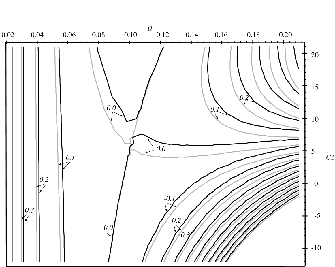
Figure 6: The fourth term of the Bjorken Sum Rule series $r_{3}^{est}a^{3}$ as predicted by the [0/2] PAP (gray line) and the PMS/ECH (black line). The separation between each pair of adjacent contours is 0.1.

The last point is the direct numerical comparison of the fourth-order terms predicted by the [0/2] Padé approximant and the PMS/ECH methods. Figure 6 displays $r_{3}^{est}(a,c_{2})a^{3}$ as calculated by the different methods, where we see excellent agreement between the [0/2] PAP and the PMS/ECH predictions for $r_{3}$ in every RS.

7 Application to the Extraction of $\alpha_{s}(M_{Z})$

To illustrate the approach described above, we now use the Bjorken sum rule [6, 7, 8] to extract a value of $\alpha_{s}(M_{Z})$ [15],[3] from the available polarized deep inelastic scattering data at $Q^{2}=3$ GeV² [16]-[20]. We do not attempt to re-evaluate the values these experiments quote for the integrals $\Gamma_{1}^{p,n}$, nor their quoted errors due, for example, to the extrapolations to $x_{Bj}=0,1$ or the modeling of the possible $Q^{2}$-dependence in $g_{1}^{p,n}(x_{Bj},Q^{2})$. Data are also available at higher values of $Q^{2}$ [21], but modeling the evolution to $Q^{2}=3$ GeV² would introduce an additional systematic error which we prefer to avoid. For our illustrative purpose, it is sufficient to use the 3 GeV² data alone. The $Q^{2}=3$ GeV² data set we use is as follows: $\displaystyle\Gamma_{1}^{n}$ $\displaystyle=$ $\displaystyle{-}0.033\,\pm\,0.006\hbox{\,(stat.)}\,\pm\,0.009\hbox{(sys.)}\hskip 100.00015pt\cite[cite]{[\@@bibref{}{E142update}{}{}]}$ $\displaystyle\Gamma_{1}^{n}$ $\displaystyle=$ $\displaystyle{-}0.032\,\pm\,0.013\hbox{\,(stat.)}\,\pm\,0.017\hbox{(sys.)}\hskip 100.00015pt\cite[cite]{[\@@bibref{}{HERMES}{}{}]}$ $\displaystyle\Gamma_{1}^{p}$ $\displaystyle=$ $\displaystyle\phantom{-}0.127\,\pm\,0.004\hbox{\,(stat.)}\,\pm\,0.009\hbox{(sys.)}\hskip 100.00015pt\cite[cite]{[\@@bibref{}{E143p}{}{}]}$ (40) $\displaystyle\Gamma_{1}^{d}$ $\displaystyle=$ $\displaystyle\phantom{-}0.042\,\pm\,0.004\hbox{\,(stat.)}\,\pm\,0.009\hbox{(sys.)}\hskip 100.00015pt\cite[cite]{[\@@bibref{}{E143d}{}{}]}$ which may be combined to yield the following combined result for the Bjorken sum rule $$\Gamma_{1}^{p}(3\hbox{GeV}^{2})-\Gamma_{1}^{n}(3\hbox{GeV}^{2})=0.160\pm 0.014$$ (41) to be compared with the theoretical calculations of both perturbative and nonperturbative (higher-twist) effects. We estimate the latter using [22]:

$$\delta(\Gamma_{1}^{p}-\Gamma_{1}^{n})={-0.02\pm 0.01\over Q^{2}}$$ (42)

As the basis for our extraction of $\alpha_{s}$, we use the ECH RS, in which the [0/2] PS coincides with the partial sum. We then translate the result to the $\overline{\hbox{MS}}\,$ RS with $\mu=Q$, so it can be easily compared with other calculations. This provides the following estimate of $\alpha_{s}$ in the $\overline{\hbox{MS}}\,$ RS at $Q^{2}=3$ GeV²:

$$a\equiv{\alpha_{s}(3\hbox{GeV}^{2})\over\pi}=0.102^{+0.010}_{-0.017}$$ (43)

where in the central value we have included the shift due to the higher-twist estimate (42). The error quoted in (43) is purely experimental, being obtained directly from our evaluation (41). This must be combined with theoretical error in the higher-twist estimate (42), $\delta_{a}(HT)=\pm 0.003$, and the theoretical error estimated from the minimum and maximum values of the [0/2] Padé in the ${\cal C}\leq 4$ region, which yields $\delta_{a}(RS)=\pm 0.004$. Thus we find

$$a\equiv{\alpha_{s}(3\hbox{GeV}^{2})\over\pi}=0.102^{+0.010}_{-0.017}\,\,{}^{+0.005}_{-0.005}$$ (44)

where the first set of errors is experimental and the second theoretical. Finally, evolving (44) to $M_{Z}$, we obtain,

$$\alpha_{s}(M_{Z})=0.117^{+0.004}_{-0.007}\,\,{}^{+0.002}_{-0.002}$$ (45)

where the extrapolation error is negligible, as discussed in [3]. The dominant source of the theoretical error is $\delta_{a}(RS)$, with a somewhat smaller contribution from $\delta_{a}(HT)$. It is interesting to compare the central value in (45) with what one would obtain as the naïve result in the $\overline{\hbox{MS}}\,$ RS: $\alpha_{s}(M_{Z})=0.123$ , which is outside the theoretical error range quoted in (45).

8 Conclusions

We have explored in this paper the relationship between Padé Approximants and the PMS and ECH techniques for estimating higher-order coefficients in perturbative QCD. The similarities between numerical results at the NNLO level may not be coincidences in certain choices of RS, as we have discussed above.

Padé summation (PS) has the remarkable property of reducing drastically the RS dependence of the perturbative series for the Bjorken sum rule with three quark flavors, if one chooses the appropriate [0/2] Padé. This observation favors the hypothesis that PS indeed leads us rapidly to the correct ‘sum’ of the perturbative QCD series. We have noted also that the Padé Approximant Prediction (PAP) for the next term in the series is quite successful, although it does not reduce the RS dependence as much as the [0/2] PS.

We believe that these results support the suggestion that Padé Approximants may be useful in applications to perturbative QCD, just as they have proved to be useful in applications to condensed-matter problems and elsewhere in quantum field theory. As an illustration how the PS technique may be useful in QCD, we have applied it to the perturbative series for the Bjorken sum rule, and used it to reduce the theoretical error associated with the choice of Renormalization Scheme (RS). Present data at $Q^{2}=3$ GeV² yield the evaluation (45), in which the theoretical error (given second) is considerably smaller than the experimental error (given first). This result indicates that the PS technique may enable a highly competitive value of $\alpha_{s}(M_{Z})$ to be extracted from future polarized lepton scattering data.

Acknowledgements

We thank A.B. Zamolodchikov for discussion on the asymptotic behaviour of the $\beta$ function. The work of J.E. was supported in part by the Director, Office of Energy Research, Office of Basic Energy Science of the U.S. Department of Energy, under Contract DE-AC03-76SF00098. The research of E.G. and M.K. was supported in part by the Israel Science Foundation administered by the Israel Academy of Sciences and Humanities, and by a Grant from the G.I.F., the German-Israeli Foundation for Scientific Research and Development.

Figure 1: A contour plot in the plane of RS parameters $a,c_{2}$ of the Bjorken Sum Rule effective charge $a^{*}_{Bj}$ calculated up to NNLO, i.e., the third-order partial sum. The separations between the contours are $\Delta a^{*}_{Bj}=0.002$. The values of $a,c_{2}$ in the $\overline{\hbox{MS}}\,$, PMS and ECH RS are indicated. In addition, we plot contours of the Cancellation Index: ${\cal C}=2,3,4,5$.

Figure 2: A contour plot of the RS dependence of the Bjorken Sum Rule effective charge $a^{*}_{Bj}$ calculated using [0/2] Padé Summation. The $a^{*}_{Bj}$ and ${\cal C}$ contours are spaced as in Fig. 1. The larger separations between the $a^{*}_{Bj}$ contours reflect the reduced RS dependence compared with the third-order partial sum shown in Fig. 1.

Figure 3: The RS dependence of the Bjorken Sum Rule effective charge $a^{*}_{Bj}$ calculated using [1/1] Padé Summation. We see in this three-dimensional plot peaks corresponding to RS’s for which the [1/1] PS is particularly erratic, signalling its unreliability.

Figure 4: A contour plot of the RS dependence of the Bjorken Sum Rule effective charge $a^{*}_{Bj}$ calculated using a fourth-order partial sum evaluated with the [0/2] PAP fourth-order coefficient. The $a^{*}_{Bj}$ contours are spaced as in Fig. 1, and we also show the ${\cal C}=4$ contour.

Figure 5: A contour plot of the RS dependence of the Bjorken Sum Rule effective charge $a^{*}_{Bj}$ calculated using a fourth-order partial sum evaluated with the PMS/ECH fourth-order coefficient. The $a^{*}_{Bj}$ contours are spaced as in Fig. 1, and we also show the ${\cal C}=4$ contour.

References

- [1] M.A. Samuel, G. Li and E. Steinfelds, Phys. Rev. D48(1993)869 and Phys. Lett. B323(1994)188; M.A. Samuel and G. Li, Int. J. Th. Phys. 33(1994)1461 and Phys. Lett. B331(1994)114.
- [2] M.A. Samuel, J. Ellis and M. Karliner, Phys. Rev. Lett. 74(1995)4380.
- [3] J. Ellis, E. Gardi M. Karliner and M.A. Samuel, Phys. Lett. B366(1996)268.
- [4] P.M. Stevenson, Phys. Rev. D23(1981)2916.
- [5] G. Grunberg Phys. Rev. D29(1984)2315.
- [6] J. Bjorken, Phys. Rev. 148(1966)1467; D1(1970)1376.
- [7] J. Kodaira et al., Phys. Rev. D20(1979)627; J. Kodaira et al., Nucl. Phys. B159(1979)99.
- [8] S.A. Larin, F.V. Tkachev and J.A.M. Vermaseren, Phys. Rev. Lett. 66(1991)862; S.A. Larin and J.A.M. Vermaseren, Phys. Lett. B259(1991)345.
- [9] C.N. Lovett-Turner and C.J. Maxwell, Nucl. Phys. B432(1994)147.
- [10] A.L. Kataev and V.V. Strashenko Mod. Phys. Lett. A10 (1995) 235.
- [11] P. A. Ra̧czka Z. Phys. C65 (1995) 481. hep-ph/9407343.
- [12] S.J. Brodsky, G.P. Lepage and P.M. Mackenzie, Phys. Rev. D28(1983)228; S.J. Brodsky and H.J. Lu, Phys. Rev. D51(1995)3652.
- [13] S.J Brodsky, J. Ellis, E. Gardi, M. Karliner and M.A. Samuel, in preparation.
- [14] M.A. Samuel, J. Ellis, E. Gardi and M. Karliner, in preparation.
- [15] J. Ellis and M. Karliner, Phys. Lett. B341(1995)397.
- [16] E142 Coll., P.L. Anthony et al., Phys. Rev. Lett. 71(1993)959;
- [17] G.G. Petratos, on behalf of the E142 Coll., Kent State U. report KSUCNR-06-96, talk at the XIV PANIC conference, Williamsburg, Virginia, May 1996.
- [18] E143 Coll., K. Abe et al., Phys. Rev. Lett. 74(1995)346.
- [19] E143 Coll., K. Abe et al., Phys. Rev. Lett. 75(1995)25;
- [20] HERMES Coll., preliminary results reported at DIS ’96 conference in Rome and at http://dxhra1.desy.de:80/first_g1.ps .
- [21] EMC Coll., J. Ashman et al., Phys. Lett. B206(1988)364; Nucl. Phys. B328(1989)1; SMC Coll., B. Adeva et al., Phys. Lett. B302(1993)533; SMC Coll., D. Adams et al., Phys. Lett. B329(1994)399; SMC Coll., D. Adams et al., Phys. Lett. B357(1995)248; A. Deshpande, on behalf of SMC Coll., lecture at QCD ’96, 4-12 Jul 1996 , Montpellier, France.
- [22] I.I. Balitsky, V.M. Braun and A.V. Kolesnichenko, Phys. Lett. B242(1990)245; erratum: ibid, B318(1993)648. B. Ehrnsperger, A. Schaefer and L. Mankiewicz, Phys. Lett. B323(1994)439; G.G. Ross and R.G. Roberts, Phys. Lett. B322(1994)425; E. Stein et al., Phys. Lett. B343(1995)369; E. Stein et al., Phys. Lett. B353(1995)107; V.M. Braun, QCD Renormalons and Higher Twist Effects, Proc. Moriond 1995, hep-ph/9505317. See also discussion pertaining to eq. (7) in Ref. [15].