On the Possibility to Study Color Transparency in the Large Momentum Transfer Exclusive $d(p,2p)n$ Reaction

Abstract

The deuteron disintegration at high energies and large angles in the $d(p,2p)n$ reaction, is calculated in kinematical conditions where the dominant contributions are due to soft rescatterings of the initial and final nucleons, which accompany the hard $pp$ reaction. The eikonal approximation, which accounts for relativistic kinematics as dictated by Feynman diagrams, reveals the important role played by the initial and final state interactions in the angular and momentum dependences of the differential cross section. Based on these results, we propose a new and effective test, at moderate energies, of the physics relevant for the color transparency phenomenon in hadron-initiated exclusive hard processes.

I Introduction

We have demonstrated recently [1] that it is possible to regulate the relative contributions of different reaction mechanisms in the exclusive high energy hard $pd\rightarrow ppn$ reaction, by selecting specific kinematical conditions. In that paper we discussed this reaction within the kinematics that is preferential to the study of short range nucleon correlations in the deuteron, the role of relativistic effects in the deuteron structure and the effects of nucleon binding. The aim of the present paper is to analyze the reaction in the kinematics favorable for the search of the Color Transparency (CT) phenomenon.

It has been shown in refs.[1, 2] that, under certain kinematical conditions, initial and final state interactions can dominate the cross sections. Those same kinematics can be advantageous for studying CT by the vanishing initial (ISI) and final (FSI) state interactions of hadronic products in the hard exclusive $pN$ scattering. (For details on CT physics, see Ref.[3] and references therein). As a first step for the identification of CT it is necessary to develop a baseline model which accounts for the initial and final state interactions within the conventional eikonal approximation. Thus, in this paper, we first restrict our considerations by calculating the elastic rescatterings of nucleons only. Next we will include the inelastic production in the intermediate states in terms of CT.

In Ref.[2] the high momentum transfer exclusive deuteron electro-disintegration reaction has been calculated within the eikonal approximation. The calculation of the Feynman diagrams, relevant for the propagation of knocked out energetic nucleons through the nuclear medium, revealed certain effects related to the finite longitudinal distances, which are beyond the formulae of conventional Glauber approximation[4]. One of the aims of this work is to extend the formalism of Ref.[2] to account for similar effects in the $d(p,2p)n$ reaction.

Another motivation of our study is to understand the unexpected energy dependence of the semi-inclusive $A(p,p)X$ reaction. In the energy range up to the $10~{}GeV$, Carroll et al. Ref.[5] found that, in semi-inclusive $A(p,2p)X$ reactions, the absorption of protons was reduced compared to the value predicted in the Glauber approximation. At incident proton energies larger than $10~{}GeV$ an increase in the absorption was observed. That result led to a number of theoretical suggestions, such as the possible importance of the interference between interactions of point like- and large size configurations [6], the longitudinal momentum dependence of nuclear transparency at pre-asymptotic energies[20], the possible existence of a threshold for charmed particle production [8], etc. Exploring the deuteron in the above energy range and restricting the kinematics to where the deuteron wave function is well known, may help to elucidate the physics of hadron propagation through the nuclear medium and the energy dependence of the semi-inclusive reaction.

As a definition for hard $pp$ collision in the exclusive $d(p,2p)n$ reaction we choose the conditions of large center of mass angle ($\geq 60^{0}$) $pp$ scatterings with $|t|$, $|u|$ $\geq~{}2~{}(GeV/c)^{2}$. We restrict the calculations to momenta of the incoming proton $p_{1}\geq 6~{}GeV/c$, where a reliable parameterization for hard $pp$ scattering exists (see e.g.[1]).

We deduce eikonal formulae of the scattering process by analyzing the Feynman diagrams corresponding to the single and double rescatterings(see Fig.1). At the present kinematical conditions the nonrelativistic deuteron wave function has been used but the full relativistic kinematics of the interaction is taken into account by the Feynman diagram approach. At intermediate energies we account for relativistic kinematics exactly, i.e. we keep also terms $\sim{1\over\sqrt{s}}$ whose contributions are enhanced due to the steep momentum dependence of the deuteron wave function. We make the approximation that the momentum of the fast nucleon is almost conserved in elastic high energy soft(small angle) collisions. Thus, the hard process kinematics are not strongly influenced by ISI and FSI (see Appendix B).

In section 2 we outline the details of the calculation, and explain the difference between our results and the nonrelativistic Glauber approximation. The results can be used to calculate nucleon rescatterings off any nucleus. For the deuteron we calculate analytically the scattering amplitudes, using the known (see e.g. Refs.[12, 13, 18]) parameterization of the wave function in momentum space.

In section 3 we present the results of numerical calculations for the kinematical conditions that can be reached in the EVA experiment at BNL[9]. The results reveal a strong impact of initial and final state interactions on the angular and momentum dependences of the differential cross sections. A surprising prediction is the azimuthal dependence of the final state interaction, which is a consequence of the interplay between hard $pp$ scattering and soft $pn$ rescatterings. We analyze also the range of applicability of the commonly used factorization of hard and soft scattering amplitudes. In section 3 we estimate the size of expected CT effects and suggest new options for the search for various consequences of CT. The simultaneous observation of all effects will make it possible to reach unambiguous conclusions about the onset of CT. The results will be summarized in section 4.

In Appendix A the analytical calculation of the rescattering amplitude for the deuteron is presented. In Appendix B we estimate the distortion of the kinematics of hard processes due to soft $NN$ rescatterings.

II Kinematics and approximations.

In this section we calculate the cross section for the $d(p,2p)n$ reaction in the kinematics where the deuteron is at rest and the $pp$ scattering is ”hard”. The kinematics of the reaction is determined by the four-momenta $p_{d}=(E_{d},p_{d})$, $p_{1}=(E_{1},p_{1})$, $p_{3}=(E_{3},p_{3})$, $p_{4}=(E_{4},p_{4})$, and $p_{s}=(E_{s},p_{s})$ of the deuteron, incoming and scattered protons and spectator neutron, respectively (c.f. fig.1a). We define also the variable ${\alpha_{s}}={E_{s}-p_{sz}\over m_{d}/2}$, which is convenient for the description of high energy processes. The quantity ${\alpha_{s}\over 2}$ can be viewed simply as the fraction of the deuteron momentum carried by the spectator neutron, in the infinite momentum reference frame ( in which the deuteron is fast). The indices $"t"$ and $"z"$ denote the transverse and longitudinal directions with respect to the incoming proton momentum $p_{1}$. The light cone momentum of the target proton is $\alpha=2-\alpha_{s}$. We will use also the spectator azimuthal angle $\phi_{s}$, which is the angle between the $(p_{1},p_{3})$ and $(p_{1},p_{s})$ planes.

We choose $|t|=|(p_{1}-p_{3})^{2}|\sim{s-4m^{2}\over 2}$ and $|t|$, $|u|=|(p_{1}-p_{4})^{2}|$ $\geq~{}2~{}GeV^{2}$ in order to fulfill the requirements of hard $pp$ scattering at large angles. With these kinematics, in the rest frame of the nucleus, the transverse components of the proton momenta are small compared to the longitudinal components i.e.:

$$({p_{3t}\over p_{3z}})^{2}\sim\theta^{2}_{3}\approx 2{m\over p_{1}}\alpha\ll 1;\ \ \ \ \ \ \ \ \ \ ({p_{4t}\over p_{4z}})^{2}\sim\theta^{2}_{4}\approx 2{m\over p_{1}}(2-\alpha)\ll 1$$ (1)

where $\theta_{3}$ and $\theta_{4}$ are the polar angles between the scattered/ knocked-out protons and the incoming proton ($\vec{p}_{1}$).

We restrict the kinematical region to relatively small spectator neutron momenta i.e. $\alpha_{s}=2-\alpha\approx 1$ and $p_{st}\leq 300-400~{}MeV/c$. It was shown in ref.([1]) that vacuum ($Z$)-type diagrams in the $d(p,2p)n$ reaction can be neglected under those conditions. By restricting the calculation to this range of Fermi momenta we can also neglect the contribution from possible non-nucleonic components in the deuteron wave function. As a result it is safe to use a conventional non-relativistic deuteron wave function (see e.g. Refs.([12, 13]).

Fig.1 depicts all the relevant Feynman diagrams for the impulse approximation and for the initial and final state interactions, when the soft rescatterings are calculated within the elastic eikonal approximation. The solid circles in the diagrams represent the hard $pp$ scattering amplitude and the broken lines represent the amplitude of small angle elastic NN scattering. Note that, in eikonal approximation, there can be no contribution from diagrams where a fast proton experiences soft rescatterings off both target proton and slow spectator neutron. This is due to the finite longitudinal distance between the target proton and neutron and the fact that the sequence of the projectile proton colliding off the target proton and neutron, followed by a hard $pp$ scattering is geometrically impossible. Similarly, it is easy to demonstrate that only diagrams of Fig.1 survive within a eikonal approximation. A similar cancelation of diagrams is well known in nonrelativistic quantum mechanics where infinite series over exchange by potential are reduced, in the high energy limit, to the diagrams expressed through the full amplitudes of NN scattering[14].

A The impulse approximation (IA)

We can classify the Feynman diagrams in Fig.1 by the number of soft initial and final state interactions. The simplest amplitude is the impulse approximation amplitude of Fig.1a. that can be written as:

$$F_{a}=(2\pi)^{{3\over 2}}\psi(p_{s}^{z},\vec{p}_{t})A^{hard}(s,t),$$ (2)

where $A^{hard}$ is the amplitude of the hard $pp$ scattering and $\psi$ is the nonrelativistic deuteron wave function normalized as $\int\psi^{2}(p)d^{3}p=1$. We are interested in the cross section on a deuteron normalized to the $pp$ cross section at the same $s$ and $t$, so that the hard $pp$ scattering amplitude is cancelled out.

B The single rescattering amplitude

In the eikonal approximation the first order rescattering is described by the diagrams of Fig.1b,c,d. The single rescattering amplitude ( Fig. 1b) can be parameterized as follows:

$$F_{b}={1\over\sqrt{2m}}\int{A^{hard}(s^{\prime},t)\Gamma(p_{d},p_{s})f^{pn}(p_{4},p^{\prime}_{s},p_{s})\over[p_{2}^{2}-m^{2}+i\epsilon][p^{\prime 2}_{s}-m^{2}+i\epsilon][(p_{4}+p_{s}-p^{\prime}_{s})^{2}-m^{2}+i\epsilon]}{d^{4}p^{\prime}_{s}\over i(2\pi)^{4}},$$ (3)

where, in the intermediate state, $p^{\prime}_{s}$ is the momentum of the spectator neutron, $s^{\prime}=(p_{3}+p_{4}+p_{s}-p^{\prime}_{s})^{2}$, $\Gamma(p_{d},p_{s})$ is the invariant vertex of the transitions $d\rightarrow pn$ into two off-mass shell nucleons and $f^{pn}$ is the spin dependent amplitude of $pn$ soft scattering. All spin dependences of the target nucleons is included in the vertex factor. We factorize the hard scattering amplitude $A^{hard}$ out of the integral because the transferred momenta in soft rescattering are negligible compared to the transferred momentum of the hard amplitude (The validity of this approximation is discussed in Appendix B). It is reasonable to neglect also the dependence of $f_{pn}$ on $p^{\prime}_{s0}$ (see c.f. [15]) because, at high energies, the $NN$ interaction depends only weakly on the collision energy. Using a non-relativistic description of the Fermi motion in the deuteron allows us to evaluate the loop integral by taking the residue over the spectator nucleon energy in the intermediate state i.e. we can replace $[p^{\prime 2}_{s}-m^{2}+i\epsilon]^{-1}d^{0}p^{\prime}_{s}$ by $-i(2\pi)/2E^{\prime}_{s}\approx-i(2\pi)/2m$. This is possible because in this case it is the only pole in the lower part of the $p^{\prime}_{s0}$ complex plane. The calculation of the residue in $p^{\prime}_{s0}$ fixes the time ordering from left to right in diagram Fig.1b. We introduce the nonrelativistic deuteron wave function as: $\psi(p_{d}-p^{\prime}_{s})\equiv{\Gamma^{d\rightarrow pn}\over[p^{2}_{2}-m^{2}+i\epsilon]\sqrt{(2\pi)^{3}2m}}$ (with $\int|\psi(k)|^{2}d^{3}k=1$) (see e.g.[15, 16, 17]). In the laboratory system the amplitude can be rewritten as:

$$F_{b} = -{(2\pi)^{{3\over 2}}\over 2m}A^{hard}(s,t)\int\psi(-p^{\prime}_{s}){f^{pn}(p_{4},p^{\prime}_{s},p_{s})\over[(p_{4}+p_{s}-p^{\prime}_{s})^{2}-m^{2}+i\epsilon]}{d^{3}p^{\prime}_{s}\over(2\pi)^{3}}$$ (4)

$$= -{(2\pi)^{{3\over 2}}\over 2}A^{hard}(s,t)\int\psi(-p^{\prime}_{s}){f^{pn}(p_{st}-p^{\prime}_{st})\over 2mp_{4z}[p^{\prime}_{sz}-p_{sz}+\Delta_{4}+i\epsilon]}{d^{3}p^{\prime}_{s}\over(2\pi)^{3}},$$ (5)

where

$$\Delta_{4}=(E_{s}-m){E_{4}\over p_{4z}}-(p_{st}-p^{\prime}_{st}){p_{4t}\over p_{4z}}.$$ (6)

In the last part of eq.(5) we used energy-momentum conservation to express the propagator of a proton of momentum $p_{4}$ as:

$$(p_{4}+p_{s}-p^{\prime}_{s})^{2}-m^{2}+i\epsilon=$$ (7)

$$2p_{4z}\left[p^{\prime}_{sz}-p_{sz}+(E_{s}-m){E_{4}\over p_{4z}}-(p_{st}-p^{\prime}_{st}){p_{4t}\over p_{4z}}+{(p_{s}-p^{\prime}_{s})^{2}\over 2p_{4z}}\right]$$ (8)

$$\approx 2p_{4z}[p^{\prime}_{sz}-p_{sz}+\Delta_{4}].$$ (9)

We use the fact that the energy transferred in the $pn$ rescattering is negligible compared to the total energy of the scattered particles so that we may neglect the term: ${(p_{s}-p^{\prime}_{s})^{2}\over 2p_{4z}}$ with respect to the other two contributions to $\Delta_{4}$.

We keep the term $(E_{s}-m){E_{4}\over p_{4z}}$ because it does not vanish with the increase of the projectile energy at fixed spectator nucleon momentum. We also keep the term $(p_{st}-p^{\prime}_{st}){p_{4t}\over p_{4z}}$ which decreases only as ${1\over\sqrt{p_{1}}}$ according to eq.(1). If the projectile energy is not extremely large, the contribution of this term in some kinematical conditions can be comparable in size to the first term of eq.(6).

The fact that the soft $NN$ scattering amplitude depends only weakly on the initial energy helps to simplify eq.(5). It is convenient to redefine the soft scattering amplitude: ${f^{pn}(p_{4},p^{\prime}_{s},p_{s})\over 2p_{4z}m}\approx f^{pn}(p_{s}-p^{\prime}_{s})$, where $f^{pn}$ is now the scattering amplitude normalized by the optical theorem $f^{pn}(k=0)=i\sigma^{pn}_{tot}$. We may neglect the longitudinal momentum transfer in $f^{pn}(p^{\prime}_{s}-p_{s})$ and assume that the transferred momenta are almost transverse: i.e. $p_{s}-p^{\prime}_{s}\approx p_{st}-p^{\prime}_{st}\equiv k_{t}$. Approximating the transferred longitudinal momenta, as $k_{z}\equiv p_{sz}-p^{\prime}_{sz}=\Delta_{4}$ and using the fact that in the rescattering integral the average transferred momenta in the $pn$ scattering are $\sim p_{t}$, we see that the condition $\Delta_{4}\ll|p_{t}|$ (or $|p_{s}|\ll 2m$) allows us to neglect the longitudinal momentum transfer in the soft scattering amplitude. Therefore, under our kinematical conditions, eq.(5) can be rewritten as:

$$F_{b}=-A^{hard}(s,t){(2\pi)^{{3\over 2}}\over 2}\int\psi(-p^{\prime}_{s}){f^{pn}(p_{st}-p^{\prime}_{st})\over[p^{\prime}_{sz}-p_{sz}+\Delta_{4}+i\epsilon]}{d^{3}p^{\prime}_{s}\over(2\pi)^{3}},$$ (10)

The integration in eq.(10) can be performed in coordinate space. Writing the Fourier transform of the deuteron wave function as:

$$\psi(p)={1\over(2\pi)^{{3\over 2}}}\int d^{3}r\phi(r)e^{-ipr}$$ (11)

and using the coordinate space representation of the nucleon propagator:

$${1\over[p^{\prime}_{sz}-p_{sz}+\Delta_{4}+i\epsilon]}=-i\int dz^{0}\Theta(z^{0})e^{i(p^{\prime}_{sz}-p_{sz}+\Delta_{4})z^{0}}$$ (12)

we obtain the formula for the rescattering amplitude:

$$F_{b} = -A^{hard}(s,t){1\over 2i}\int{d^{2}k_{t}\over(2\pi)^{2}}d^{3}r\phi(r)f^{pn}(k_{t})\theta(-z)e^{(p_{sz}-\Delta_{4})z}e^{(p_{st}-k_{t})b}$$ (13)

$$= -A^{hard}(s,t)\int d^{3}r\phi(r)\theta(-z)\Gamma^{pn}(\Delta_{4},-z,-b)e^{ip_{s}r}$$ (14)

where $\vec{r}=\vec{r}_{p}-\vec{r}_{n}$, $k_{t}=p_{st}-p^{\prime}_{st}$. We define a generalized profile function $\Gamma$:

$$\Gamma^{pn}(\Delta_{4},z,b)={1\over 2i}e^{-i\Delta_{4}z}\int f^{pn}(k_{t})e^{-ik_{t}b}{d^{2}k_{t}\over(2\pi)^{2}}.$$ (15)

Eq.(14) reduces to a Glauber-type approximation in the limit of zero longitudinal momentum transfer $\Delta_{4}$. The dependence of the profile function on the longitudinal momentum transfer originates from two sources. According to eqs.(6,9) the term $(E_{s}-m){E_{4}\over p_{4z}}$ accounts for the relativistic kinematics which follows from the evaluation of the propagator of a proton with momentum $p_{4}$. A similar factor was found also for the $d(e,e^{\prime}p)n$ reaction in ref.[2]. The second term $(p_{st}-p^{\prime}_{st}){p_{4t}\over p_{4z}}={k_{t}p_{4t}\over p_{4z}}$ is due to a slight misalignment of the projectile momentum with the directions of the outgoing protons. Even though, according to eq.(1), this factor is small it has a large effect on the cross section due to the steep momentum dependence of the deuteron wave function (see discussion in section 3). The same modified profile function, eq.(15), is valid for the single rescattering amplitudes off any nucleus $A$[19]. The unique feature for the deuteron is the possibility to calculate the rescattering amplitudes using an analytical parameterization of the deuteron wave function (c.f. [12, 13]).

Substituting the deuteron wave function in eq.(10) by the analytic form of eqs.(A1), (A2) and (A3), one can perform the integration over $p^{\prime}_{sz}$ by deforming the contour of integration in the upper complex half-plane of $p^{\prime}_{sz}$. We can then evaluate the integral by taking residues over corresponding poles in the deuteron wave function. The answer (see appendix A for details) for the single rescattering amplitude $F_{b}$ (eq.(10)) is:

$$F_{b}=-{(2\pi)^{{3\over 2}}\over 4i}A^{hard}(s,t)\int{d^{2}k_{t}\over(2\pi)^{2}}f^{pn}(k_{t})\left(\psi^{\mu}(\tilde{p}_{s})-i\psi^{\prime\mu}(\tilde{p}_{s})\right),$$ (16)

where $\tilde{p}_{s}\equiv\vec{\tilde{p}_{s}}(p_{sz}-\Delta_{4},\vec{p}_{st}-\vec{k}_{t})$, $\psi^{\mu}$ is deuteron wave function defined in eq.(A1) and $\psi^{\prime\mu}$ is defined in eqs.(A9) and (A11).

We can now calculate also the amplitude corresponding to the diagram of Fig.1c, replacing $p_{4}\rightarrow p_{3}$. Thus

$$F_{c}=-A^{hard}(s,t)\int d^{3}r\phi(r)\theta(-z)\Gamma^{pn}(\Delta_{3},-z,-b)e^{ip_{s}r}$$ (17)

$$=-{(2\pi)^{{3\over 2}}\over 4i}A^{hard}(s,t)\int{d^{2}k_{t}\over(2\pi)^{2}}f^{pn}(k_{t})\left(\psi^{\mu}(\tilde{p}_{s})-i\psi^{\prime\mu}(\tilde{p}_{s})\right),$$ (18)

where $\tilde{p}_{s}\equiv\vec{\tilde{p}_{s}}(p_{sz}-\Delta_{3},\vec{p}_{st}-\vec{k}_{t})$ and $\Delta_{3}$ is described by eq.(6) with the substitution $p_{4}\rightarrow p_{3}$.

The initial state interaction represented by diagram Fig1.d. is described by an equation similar to eq.(10):

$$F_{d}=-{(2\pi)^{{3\over 2}}\over 2}A^{hard}(s,t)\int\psi(-p^{\prime}_{s}){f^{pn}(p_{st}-p^{\prime}_{st})\over[p_{sz}-p^{\prime}_{sz}-\Delta_{1}+i\epsilon]}{d^{3}p^{\prime}_{s}\over(2\pi)^{3}},$$ (19)

where $\Delta_{1}$ is defined by eq.(6) with the substitution $p_{4}\rightarrow p_{1}$. In contrast to eq.(10) the singularity of the propagator in eq.(19) is now located in the upper part of the complex $p^{\prime}_{sz}$ plane. It is easy to show that, in coordinate space, this difference corresponds to the reverse sign of the argument of $\theta$ function in eq.(12): $\theta(-z)\rightarrow\theta(z)$. In momentum space, the contour of the $p^{\prime}_{sz}$ integration can be deformed in the lower complex semi-plane, where the only pole is due to singularities in the deuteron wave function at $p^{\prime}_{sz}=-i\sqrt{p^{\prime 2}_{st}+m^{2}_{j}}$ (see Appendix A) and the result of the integration differs from eq.(16) by the sign of $p^{\prime}_{sz}$ only. Thus the amplitude for diagram Fig.1d is given by:

$$F_{d} = -A^{hard}(s,t)\int d^{3}r\phi(r)\theta(z)\Gamma^{pn}(\Delta_{1},-z,-b)e^{ip_{s}r}$$ (20)

$$= -{(2\pi)^{{3\over 2}}\over 4i}A^{hard}(s,t)\int{d^{2}k_{t}\over(2\pi)^{2}}f^{pn}(k_{t})\left(\psi^{\mu}(\tilde{p}_{s})+i\psi^{\prime\mu}(\tilde{p}_{s})\right),$$ (21)

where $\tilde{p}_{s}\equiv\vec{\tilde{p}_{s}}(p_{sz}-\Delta_{1},p_{st}-k_{t})$.

C The double rescattering amplitude

The second order rescatterings where both protons scatter off the spectator neutron are represented in the diagrams of Fig. 1e,f,g and h. Using the same approach as for the single rescattering, the double rescattering amplitude of Fig.1e can be written as:

$$F_{e}={(2\pi)^{{3\over 2}}A^{hard}(s,t)\over 8}\int\psi(-p^{(1)}_{s}){f^{pn}(p^{(2)}_{st}-p^{(1)}_{st})\over[p^{(2)}_{sz}-p^{(1)}_{sz}-\Delta_{1}+i\epsilon]}{f^{pn}(p_{st}-p^{(2)}_{st})\over[p^{(2)}_{sz}-p_{sz}+\Delta_{3}+i\epsilon]}{d^{3}p^{(1)}_{s}\over(2\pi)^{3}}{d^{3}p^{(2)}_{s}\over(2\pi)^{3}}$$ (22)

where $p^{(1)}_{s}$ and $p^{(2)}_{s}$ are the spectator (neutron) momenta before the first and second rescatterings, respectively.

Since the deuteron wave function in eq.(22) does not dependent on $p^{(2)}_{s}$, the whole dependence on $p^{(2)}_{sz}$ is contained in the two propagators only. But the poles of these propagators in the $p^{(2)}_{sz}$ complex plane are located in the lower semi-plane. Due to fast convergence of the integral, the contour of integration can be moved to the upper complex semi-plane which makes the integral equal to $0$. In the coordinate space this result has a simple geometrical interpretation. The diagram describes an interaction of incoming and scattered protons with a spectator neutron which would be located simultaneously before and after the target proton which is not possible geometrically. Indeed using the coordinate representation of the deuteron wave function (eq.(11)) and the nucleon propagators (eq.(12)), we can obtain the $\Theta(z)\Theta(-z)$ term in the integrand in the coordinate space. The same reasoning leads also to zero for the amplitudes of diagrams Fig 1.f, which can be obtained from diagram Fig 1.e by substituting $p_{3}\rightarrow p_{4}$. The amplitude in diagram Fig. 1g, within the approximations discussed above takes on the form:

$$F_{g}={(2\pi)^{{3\over 2}}\over 8}\int\psi(-p^{(1)}_{s}){f^{pn}(p^{(2)}_{st}-p^{(1)}_{st})\over[p^{(1)}_{sz}-p^{(2)}_{sz}+\Delta_{3}+i\epsilon]}{f^{pn}(p_{st}-p^{(2)}_{st})\over[p^{(2)}_{sz}-p_{sz}+\Delta_{4}+i\epsilon]}{d^{3}p^{(1)}_{s}\over(2\pi)^{3}}{d^{3}p^{(2)}_{s}\over(2\pi)^{3}}$$ (23)

where $\Delta_{3}=(E^{(2)}_{s}-m){E_{3}\over p_{3z}}-(p^{(2)}_{st}-p^{(1)}_{st}){p_{3t}\over p_{3z}}$ and $\Delta_{4}=(E_{s}-E^{(2)}){E_{4}\over p_{4z}}-(p_{st}-p^{(2)}_{st}){p_{4t}\over p_{4z}}$ are different from those for single rescattering (eq.(6)). However, in our kinematics $E_{s}-E^{(2)}_{s}\sim{|k_{t}|p_{S}\over E_{s}}\ll m$ and $\Delta_{3}$, $\Delta_{4}$ can be taken to be the same as for single rescattering. Using eqs.(11) and eq.(12) one can write the amplitude, in coordinate representation, as follows:

$$F_{(g)}={1\over 2}\int d^{3}r\phi(r)\theta(-z)\Gamma^{pn}(\Delta_{3},-z,-b)\Gamma^{pn}(\Delta_{4},-z,-b)e^{ip_{s}r},$$ (24)

where $\Gamma^{pn}$ is defined by eq.(15). The difference between eq.(24) and the conventional nonrelativistic Glauber approximation is the presence of the terms $\Delta_{3}$, $\Delta_{4}$. The integration in eq.(23) over the longitudinal components of nucleon momenta $p^{(1)}_{sz}$ and $p^{(2)}_{sz}$ in the intermediate states can be evaluated by the technique used in Sec.2.2 for the calculation of the single rescattering amplitude(see Appendix A). First, we integrate over $p^{(2)}_{sz}$ by closing the contour of integration at one of the poles in the complex plane (they are located now in different semi-planes) to obtain:

$$F_{g}={-i(2\pi)^{{3\over 2}}\over 8}\int\psi(-p^{(1)}_{s}){f^{pn}(k^{(1)}_{t})\over[p^{(1)}_{sz}-p_{sz}+\Delta_{3}+\Delta_{4}+i\epsilon]}f^{pn}(k^{(2)}_{t}){d^{2}k^{(1)}_{s}\over(2\pi)^{2}}{dp^{(1)}_{sz}\over 2\pi}{d^{2}k^{(2)}_{s}\over(2\pi)^{2}}$$ (25)

The $p^{(1)}_{sz}$ integration in eq.(25) can be performed in a way similar to the one used in eq.(10) for $\Delta=\Delta_{3}+\Delta_{4}$. Therefore, we may use the result of the calculation of single rescattering to obtain:

$$F_{g}=-{(2\pi)^{{3\over 2}}\over 16}\int{d^{2}k^{(1)}_{t}\over(2\pi)^{2}}{d^{2}k^{(2)}_{t}\over(2\pi)^{2}}f^{pn}(k^{(1)}_{t})f^{pn}(k^{(2)}_{t})\left(\psi^{\mu}(\tilde{p}_{s})-i\psi^{\prime\mu}(\tilde{p}_{s})\right),$$ (26)

where $\tilde{p}_{s}\equiv\vec{\tilde{p}_{s}}(p_{sz}-\Delta_{4}-\Delta_{3},p_{st}-k^{(1)}_{t}-k^{(2)}_{t})$. The expression is symmetric under interchange of $\Delta_{4}\leftrightarrow\Delta_{3}$. Thus, for the amplitude of diagram Fig1.g we get:

$$F_{h}=F_{g}$$ (27)

D The cross section in DWIA

In the approximation where the hard $pp$ scattering amplitude is factorized (Appendix B) the cross section of the $d(p,2p)n$ reaction can be written in a form which is similar to the distorted wave impulse approximation (DWIA). Hence the cross section for $d(p,2p)n$ reaction can be expressed as follows (see e.g. Ref.[1]):

$$\frac{d^{6}\sigma^{DWIA}}{(d^{3}p_{3}/E_{3})(d^{3}p_{4}/E_{4})}={1\over 2\pi}{s^{2}-4m^{2}s\over 2m\cdot|\vec{p}_{1}|}\frac{d\sigma}{dt}^{pp}\cdot n(p_{s})\delta(E_{s}-(M_{D}-E))$$ (28)

where $E=E_{3}+E_{4}-E_{1}$. The function $n(p_{s})$ describes the distorted momentum dependence of a nucleon in the deuteron:

$$n(p_{s})={|F_{a}+F_{b}+F_{c}+F_{d}+F_{g}+F_{h}|^{2}\over|A^{hard}|^{2}(2\pi)^{3}}.$$ (29)

The factor $(2\pi)^{3}$ follows from the phase space factor of the spectator nucleon wave function. In eq(28) we neglected the virtuality of the interacting nucleon and used for $\frac{d\sigma}{dt}^{pp}$ the experimentally measured cross section and for which a phenomenological parameterization is given in Refs.[28, 6, 1].

III Numerical estimates

We wish to calculate the quantity $T$- ”Transparency” which accounts for the effects due to soft rescatterings. Traditionally (see e.g.[21]) $T$ is defined as the ratio of the experimentally measured cross section to the calculated IA cross section, which according to our definitions is:

$$T\equiv{\sigma^{DWIA}\over\sigma^{IA}}={|F_{a}+F_{b}+F_{c}+F_{d}+F_{g}+F_{h}|^{2}\over|F_{a}|^{2}}.$$ (30)

For our numerical estimates we will use the kinematics of on-shell $90^{0}$ center of mass angle $pp$ scattering. This is achieved by imposing the condition

$$t={4m^{2}-s\over 2}$$ (31)

on $s=(p_{3}+p_{4})^{2}$ and $t=(p_{1}-p_{3})^{2}$:

A Calculation within the elastic eikonal approximation

We shall call ”elastic eikonal”, the approximation where nucleons only propagate through the deuteron and soft $pn$ rescatterings are described by the diffractive $f^{pn}$ scattering amplitude. Since in the relevant kinematics the amplitude $f^{pn}$ is predominantly imaginary, the IA (eq.(2)) and double rescattering amplitudes (eq.(26)) are positive, while the single rescattering amplitudes (eqs(16), (18), (21)) are negative. Therefore the terms in eq.(30) have different signs and, depending on the kinematics, the soft rescattering terms can either increase or decrease the transparency $T$, leading to large ISI/FSI effects on the overall cross section. In Refs.[1],[2] we demonstrated that the ISI/FSI is largest for perpendicular kinematics, where the polar angle of the neutron-$\theta_{s}$ is almost perpendicular to the reaction axis. In Fig.2 we show the spectator angular ($\theta_{s}$) dependence of the transparency $T$, for different spectator momenta $p_{s}$. The calculation was done by adopting the standard parameterization for the diffractive $pn$ scattering amplitude:

$$f^{pn}=\sigma^{pn}_{tot}(i+a_{n})e^{-b_{n}k_{t}^{2}/2},$$ (32)

In our kinematics, the parameter values $\sigma^{pn}_{tot}\approx 40~{}mb$, $a_{n}\approx-0.2$ and $b_{n}\approx~{}8~{}GeV^{-2}$ were obtained by fitting the experimental $pn$ scattering data[24]. The rather weak dependence of $\sigma_{tot}$ and $b_{n}$ on the nucleon momentum, for energies above $3~{}GeV$, has been included.

The results, presented in Fig.2, confirm the large ISI/FSI effects in perpendicular kinematics. They reveal also the importance of the above discussed modifications in the conventional Glauber approximation[4]. We find that the dominant effect is due to non-zero transverse momenta of the emerging fast protons ($\sim k_{t}{p_{3,4t}\over p_{3,4z}}$). This effect reduces strongly the contribution from the interference of two rescattering amplitudes. In Fig.3 we show the $p_{t}$ dependence of $T$ at fixed value of $\alpha_{s}=1$. It follows from this figure that in the range $p_{t}<200MeV/c$ the ISI and FSI significantly screen the cross section. It is small compared to the cross section calculated within the IA approximation. The interference between single rescattering and the IA term dominates the overall scattering amplitude. With increasing $p_{t}$ $>250-300MeV/c$ the squared terms and the interferences between single rescattering amplitudes dominate and as a result $T$ may exceed $1$. At even higher $p_{t}$ the second order (negative) terms in eq.(30) (e.g. interference between single and double rescattering terms) tend to suppress the rise of $T$, thus changing the slope of the $p_{t}$ dependence.

Since at fixed $\theta_{c.m.}$, $\theta_{3}$ and $\theta_{4}$ depends on the incoming proton energy (see eq.(1)), the formulae of eikonal approximation could lead to some energy dependence of T for fixed spectator momentum, even if $\sigma^{pn}_{tot}$, $b_{n}$ were energy independent. This dependence is more noticeable for the larger momenta of the spectator, since the contribution from ISI/FSI diagrams increases with increasing $p_{t}$ (see Fig.4). In fact, we see in Fig.4 that $T$ does not depend much on incident beam energy.

Another nontrivial consequence of the interplay of hard $pp$ scattering and soft $pn$ rescattering is the dependence of FSI on the azimuthal angle of the spectator neutron. The effect is due to two important features of the reaction: in hard $pp$ scatterings protons are produced at small but finite $\theta_{3}$ and $\theta_{4}$ angles (lab) and high energy soft $pn$ rescattering is characterized by an average transferred momentum $<k^{2}>\sim p^{2}_{t}$, which is perpendicular to the trajectory of the protons. To visualize the origin of the azimuthal dependence let us compare the kinematics when the spectator has $\alpha=1$, $p_{s}\approx p_{t}$ and $\phi_{s}=180^{0}$ (in plane kinematics) and when $\alpha=1$, $p_{s}\approx p_{t}$ and $\phi_{s}=90^{0}$ (out of plane kinematics). Estimating the contribution of FSI amplitude from rescattering diagrams Fig.1b,c it is easy to show that the difference between the $\tilde{p}_{s}$ for eq.(18) is:

$$[\tilde{p}^{2}_{s}]^{(in\ plane)}-[\tilde{p}^{2}_{s}]^{(out\ plane)}\approx\Delta_{4}^{2}(\Delta_{3}^{2})\approx<k^{2}>{2m\over p_{1}}\sim<p_{t}^{2}>{2m\over p_{1}}.$$ (33)

Since the deuteron wave function depends strongly on momentum, the difference in the argument of the wave function leads to a significant effect in the dependence on azimuthal angle. Therefore the FSI interaction for out-of-plane kinematics is larger than for in-plane kinematics. This is illustrated in Fig.5 where the $\phi_{s}$ dependence of transparency $T$ is calculated at $\alpha=1$ for different values of the spectator transverse momenta $p_{t}$.

Let us discuss briefly the reliability of the derived picture within the eikonal approximation. The effects of the order of ($\sim{1\over\sqrt{s}}$) are included in the argument of the deuteron wave function. In perpendicular kinematics the deuteron wave function is sensitive to the momentum $\tilde{p}\sim 0$. Thus $\sim{1\over\sqrt{s}}$ effects are amplified by the steep momentum dependence of the deuteron wave function at small momenta. In Ref.[1] we demonstrated that the off-shell effects are minimal for the perpendicular kinematics since the $s$ dependence of the hard $pp$ scattering in this case is minimal. For the kinematics where soft rescatterings dominate (at $\alpha_{s}\approx 1$), the calculations are practically insensitive to relativistic effects in the deuteron wave function [2]. A practical conclusion is that the kinematical restriction $\alpha\approx 1$ and $p_{t}<350-400~{}MeV/c$ opens a possibility to investigate reliably effects which are sensitive to initial and final state interactions of energetic protons with the slow spectator neutron. Another important question is the validity of the factorization of hard and soft scatterings. We demonstrate in Appendix B that the errors due to this factorization are minimal for small values of the spectator transverse momenta and $\alpha_{s}\geq 1$. The numerical estimates of the errors are shown in Fig.12, which shows that, in the region of $0.9<\alpha_{s}<1.1$ and $p_{t}\leq 400~{}MeV/c$, the factorization approximation is valid within an accuracy of better than $15\%$ for energies $p_{1}\geq 6~{}GeV/c$. The accuracy improves at higher incident energies (as shown in Fig.12, for calculations at $p_{1}=6~{}GeV/c$ and $15~{}GeV/c$.)

B Implication for color transparency

The aim of the paper is to explore whether the hard exclusive $d(p,2p)n$ reaction can initiate effects of color transparency. The main idea is that at the point of interaction the hadrons of the hard elastic scattering are in a ”point like” configuration (PLC) whose subsequent strong interaction is reduced.[22, 23, 3, 21]. As a result soft interactions shortly before and after the hard collision will be lower than the usual strong interaction of hadrons. Since a PLC, produced in the hard process, is not an eigenstate of the QCD Hamiltonian but rather a wave-packet of destructively interfering mass states, it has to evolve eventually into a final hadron state. Due to time dilation, the characteristic distances for the evolution of a PLC to the normal hadronic state increases with the total energy of the PLC.

The exclusive $d(p,2p)n$ reaction has several features which are very sensitive to CT. Since ISI/FSI occur at internucleon distances in the deuteron of about $\sim 1~{}Fm$[2], one can use the spectator neutron to tag the PLC at an early stage of evolution thus reducing expansion effects. As a result, large CT effects can be expected even at comparatively low energies. Large spectator momenta $p_{s}$ with $\alpha_{s}\approx 1$ ensure small impact parameters for soft $pn$ rescatterings. This will enhance the ISI/FSI contribution to the $d(p,2p)n$ cross section.

We calculate $T$ of eq.(30) in a model which accounts for PLC formation and its time development in the framework of the quantum diffusion model (QDM)[10]. We note that CT in the resonance basis representation of PLC[11] predicts rather similar effects[2]. We follow the procedure described in ref.[25] to calculate the $pn$ scattering amplitude and profile function of eq.(15)) within QDM[10]. The $pn$ scattering amplitude $f^{pn}$ in eq.(14), (18), (21), and (24) is replaced by a position dependent one:

$$f^{PLC,N}(z,k_{t},t)=i\sigma_{tot}(z,t)\cdot e^{-{b_{n}\over 2}k^{2}_{t}}{G_{N}(t\cdot\sigma_{tot}(z,t)/\sigma_{tot})\over G_{N}(t)},$$ (34)

where $G_{N}(t)$ is the Sachs form factor, $\sigma_{tot}(z,t)$ is the effective total cross section of the interaction of the PLC at distance $z$ from the interaction point. According to ref. [10]:

$$\sigma_{tot}(z,t)=\sigma_{tot}^{pn}\left\{\left({z\over l_{h}}+{\langle r_{t}(t)^{2}\rangle\over\langle r_{t}^{2}\rangle}(1-{z\over l_{h}})\right)\Theta(l_{h}-z)+\Theta(z-l_{h})\right\},$$ (35)

where ${l_{h}=2p/\Delta M^{2}}$, with ${\Delta M^{2}=0.7-1.1GeV^{2}}$. Here ${\langle r_{t}(t)^{2}\rangle}$ represents the transverse size of the initially produced configuration. Theoretical analysis of realistic models of a nucleon indicate[21] that this size is rather small even for $|t|~{}\geq~{}1.5~{}GeV^{2}$. Any effects of interplay between large and small size configurations can be included in a rather straightforward manner[8, 6]. However our aim here is primarily to demonstrate sensitivity to CT.

The QDM calculation should be compared with the elastic eikonal calculation of the previous section, where $pn$ soft rescattering was taken to be practically energy independent (see eq.(32)). In order to emphasize any color transparency effects, we calculate again the dependence of $T$ on the spectator transverse momentum, azimuthal angle and incoming proton momentum, since we showed in Sec.3.1 that all these quantities are rather sensitive to the soft $pn$ interactions. In Fig.6, we present the $p_{t}$ dependence of $T$ (eq.(30)) calculated in the eikonal model with eq.(32) and in the QDM for the rescattering amplitude with eqs.(34,35). The shaded areas correspond to the range of the parameter $\Delta M^{2}=0.7-1.1~{}GeV^{2}$ which characterizes the scale of excitation energies in PLC and which controls the distance over which the PLC evolves to the normal hadronic state. Large values of $\Delta M^{2}$ correspond to small deviations from the elastic eikonal prediction. Fig.6 also shows that, at fixed initial energy, CT effects become more prominent with increasing $p_{t}$. This can be understood by the fact that the contribution of the IA amplitude is small and the soft rescatterings occur at small internucleon distances leading to some suppression in expansion of PLC. Also, higher order rescatterings are more important at larger $p_{t}$. They are proportional to higher powers of $\sigma^{tot}_{pn}(z,t)$ and therefore should be more suppressed by the onset of CT. The dependence of $T$ on the azimuthal angle of the spectator, in the $\alpha=1$ kinematics, is shown in Fig.7. The ISI (Fig.1d) does not contribute to the $\phi_{s}$ dependence because we chose the $z$ axis (lab) in the $p_{1}$ direction. We see in Fig.7 that the onset of CT in the $\phi_{s}$ dependence requires larger projectile energies. This is because the CT impacts the FSI only at energies $p_{3}\sim p_{4}\sim p_{1}/2$. At energies ($\sim 6~{}GeV$), before the onset of CT, the $\phi$ dependence can be used to check predictions of the elastic eikonal approximation.

To discuss the energy dependence of $T$ we include in our consideration also the models which accounts for both the PLC and large (Blob) size configurations in hard scattering $pp$ amplitude. We follow to the prescription of Ref.[26] and represent the hard $pp$ scattering amplitude as:

$$A^{Hard}(s,t)=A^{PLC}(s,t)+A^{BLC}(s,t).$$ (36)

$A^{PLC}(s,t)$ is the component of hard scattering amplitude which produces the PLC and leads to CT. $A^{BLC}(s,t)$ corresponds to the large size (soft) component of $pp$ scattering amplitude and has a cross section comparable to $\sigma_{total}$. The source of such a soft component could be either the opening of $c\bar{c}$ channels at energies near threshold[8] or the presence of Landshoff processes in hard $pp$ scattering[6]. Implications of both mechanisms for CT were discussed in details in Ref.[26], where PLC expansion effects are accounted for within the multi resonance expansion model of CT. In the present calculation we describe the expansion effects within QDM using the same Ralston-Pire parameterization for $A^{BLC}(s,t)\cite[cite]{[\@@bibref{Number}{RP}{}{}]}$. The numerical results of the multi resonance model and QDM for CT in $(p,2p)$, and $(e,e^{\prime}p)$ reactions are very close [3]. In Fig.8 we present the energy dependence of $T$ at two values of $p_{st}=0.2~{}GeV/c$ and $p_{st}=0.4~{}GeV/c$. It shows that the higher the spectator transverse momentum, the larger is the CT effect. The increase of the incoming energy of the proton diminishes the sensitivity of $T$ to $\Delta M^{2}$, due to reduced sensitivity to the expansion. The model which accounts for the interference between large and small size components of hard $pp$ scattering, as expected, reveal oscillation with the increase of projectile energy. New feature is that amplitude of these oscillations increase with $p_{t}$ and the phases of oscillations are opposite for kinematics dominated by screening ($p_{t}=0.2~{}GeV/c$) and by rescattering ($p_{t}=0.4~{}GeV/c$) effects of ISI/FSI.

As we have seen in Sec.3.1, $T<1$ at $p_{st}\lesssim 0.2GeV/c$, and $T>1$ at $p_{st}\gtrsim 0.3~{}GeV/c$, (see, Figs.3,6,8). Since, by definition, $T=1$ means complete transparency (i.e. no ISI/FSI) CT produces opposite trends in the regions where $T<1$ and $T>1$ (see e.g. Fig.6b). This property calls for a more sensitive quantity to characterize CT [2, 25]. We define the ratio:

$$R={\sigma(p^{(1)}_{st})\over\sigma(p^{(2)}_{st})},$$ (37)

where $p^{(1)}_{st}$ and $p^{(2)}_{st}$ are such that $T(p^{(1)}_{st})>1$ and $T(p^{(2)}_{st})<1$. This ratio is more sensitive to CT due to different trends of CT effects in the numerator and denominator of $R$ while it will be less sensitive to uncertainties in the theoretical calculations. In Fig.9 we present the energy dependence of $R$, which shows deviations of QDM prediction from the eikonal approximation, in the range of the initial proton momenta $\geq 6~{}GeV/c$, by a factor $2-3$ due to CT. Because of opposite phases of energy oscillations within the models which accounts for the interference between BLC and PLC (Fig.8), $R$ reveals profound oscillations in Fig.9. The dependence of $R$ on the azimuthal angle of the spectator - Fig.10 at fixed energies of initial proton could be used as a complementary method in the study of CT. Due to large FSI in the out-of-plane kinematics, the QDM prediction of CT at $p_{1}=15~{}GeV/c$ could be enhanced by the factor of $5-6$ over the eikonal results.

It was shown in Ref.[27] that IA is strongly suppressed for inelastic recoil final states in the deuteron fragmentation region. This was due to the fact that under those circumstances the IA is controlled by the inelastic component of the deuteron ground state, which is negligible for recoil momenta $\leq 700~{}MeV/c$. Thus the cross section is dominated by the rescattering diagrams. Therefore the CT will manifest itself by a reduced production of low momentum inelastic states in the deuteron fragmentation region at increasing projectile energies. In Fig.11 we present the calculation of the ratio of the cross section of quasielastic $d(p,2p)n$ reaction to that of $d(p,2p)N^{*}(1580)$ reaction. The calculations are done in the QDM and the elastic eikonal approximation [27]. Fig.11 reveals a strong sensitivity of the ratio to CT. For incident momenta from $6-18GeV/c$ the eikonal approximation shows a drop in the ratio of $10\%$, while the inclusion of CT leads to a decrease by a factor of $3$. This suggests a very simple method for studying CT effects i.e. the measurement of the energy dependence of quasielastic and inelastic rates in the deuteron fragmentation region.

IV Summary

We calculated the cross section of hard exclusive $d(p,2p)n$ reaction taking into account the initial and final state interactions, within the elastic eikonal approximation. Analysis of Feynman diagrams in the relativistic domain produced significant effects beyond the conventional nonrelativistic Glauber type formulae. The results can be applied to any nucleus. The deuteron calculations were done analytically using a well known form of the deuteron wave function.

The calculation produced a diffractive pattern in the cross section due to ISI/FSI. In the kinematics where $\alpha_{s}\approx 1$, $p_{st}\leq 0.2~{}GeV/c$ the ISI/FSI suppress the cross section with respect to IA, while at $\alpha_{s}\approx 1$ $p_{st}\geq 0.3~{}GeV/c$ the ISI/FSI increases the cross section. Another result is the prediction of an azimuthal angle dependence due to FSI. This is a result of including small but finite angles of the scattered protons into the soft rescattering amplitude. We estimated the validity of the factorization approximation within the elastic eikonal approach. We found that the factorization approximation is valid for $\alpha_{s}\approx 1$ to better than $15\%$ for $p_{st}\leq 0.4~{}GeV/c$.

Since ISI/FSI dominate the cross section in $d(p,2p)n$, the CT phenomenon will be best observed in this reaction. We calculated the transparency $T$ with the quantum diffusion model and model where the interference between small and large size components of large angle $pp$ scattering are taken into account explicitly. Exploiting the fact that CT leads to opposite effects in the kinematical regions where $T<1$ and $T>1$, we introduced the ratio $R={\sigma(T>1)\over\sigma(T<1)}$, which reveals extra sensitivity to CT effect. At presently accessible energies, the predictions of energy and angular dependences of $R$ differ by as much as a factor of 2-6 between the eikonal and CT calculations. The model with the interference of large and small size configurations predicts profound oscillations for the energy dependence of $R$.

An additional possibility to search for CT was found. It consists of measuring the energy dependence of the ratio of the production rates of elastic and inelastic recoil states in the deuteron fragmentation region. While conventional calculation predict practically no energy dependence, the CT predicts a significant drop of this ratio with increasing the projectile energies.

V Acknowledgments

We are grateful to Jonas Alster for valuable comments and for reading the manuscript. We would like to thank Jerry Miller for useful discussions and for providing his calculation of large angle $pp$ scattering amplitude. We wish to thank also Alan Caroll, Steve Heppelmann, Yael Mardor and Israel Mardor for helpful discussions. Two of us (M.S. & M.S.) thank the DOE Institute for Nuclear Theory at the University of Washington for its hospitality and support during the workshop “Quark and Gluon Structure of Nucleons and Nuclei”, where part of this work was carried out.

This work was supported, in part, by the Basic Research Foundation administrated by the Israel Academy of Science and Humanities, by the U.S.A. - Israel Binational Science Foundation Grant No. 9200126 and by the U.S. Department of Energy under Contract No. DE-FG02-93ER40771.

A Analytic calculation or rescattering amplitude

We calculate the rescattering amplitude in eq.(10) by the method described in ref.[2] using the deuteron wave function in momentum space, defined as[18]:

$$\psi^{\mu}(p)={1\over\sqrt{4\pi}}\left(u(p)+w(p)\sqrt{1\over 8}S(p_{z},p_{t})\right)\chi^{\mu}$$ (A1)

where $\chi^{\mu}$ is the deuteron spin function and

$$S(p_{z},p_{t})={3(\vec{\sigma}_{p}\cdot\vec{p})(\vec{\sigma}_{n}\cdot\vec{p})\over p^{2}}-\vec{\sigma}_{p}\cdot\vec{\sigma}_{n}$$ (A2)

where $\sigma_{p}$, $\sigma_{p}$ Pauli matrices. The functions $u(p)$ and $w(p)$ are the radial wave functions of $S$- and $D$- states, respectively and they can be written as[12, 13]:

$$u(p)=\sum\limits_{j}{c_{j}\over p^{2}+m^{2}_{j}};\ \ \ \ \ \ \ \ w(p)=\sum\limits_{j}{d_{j}\over p^{2}+m^{2}_{j}}$$ (A3)

where $\sum\limits_{j}c_{j}=\sum\limits_{j}d_{j}=0$, which guarantees that $u(p),w(p)\sim{1\over p^{4}}$ at large $p$ and $\sum\limits_{j}{d_{j}\over m^{2}_{j}}=0$ to provide $w(p=0)=0$. Insertion of eq.(A3) into the eq.(10) gives:

$$F_{b}=-{(2\pi)^{{3\over 2}}\over 2}\sum\limits_{j}A^{hard}(s,t)\int{d^{2}p^{\prime}_{st}\over(2\pi)^{2}}f^{pn}(k_{t})$$ (A4)

$$\times\int{dp^{\prime}_{sz}\over(2\pi)}\left({c_{j}\over p^{\prime 2}_{s}+m^{2}_{j}}+{d_{j}\over p^{\prime 2}_{s}+m^{2}_{j}}\sqrt{1\over 8}S(p^{\prime}_{sz},p^{\prime}_{st})\right){\chi^{\mu}\over p^{\prime}_{sz}-p_{sz}+\Delta_{4}+i\epsilon}$$ (A5)

Substituting $p^{\prime 2}_{s}+m^{2}_{j}=(p^{\prime}_{sz}+i\sqrt{m_{j}^{2}+p^{\prime 2}_{st}})(p^{\prime}_{sz}-i\sqrt{m_{j}^{2}+p^{\prime 2}_{st}})$ one can perform the integration over $p^{\prime}_{sz}$ by closing the contour in the upper $p^{\prime}_{sz}$ complex semi-plane. Note that the $p^{-2}$ dependence of the tensor function $S(p)$ will not introduce a new singularity, since $w(p=0)=0$. Setting the residue at the point $p^{\prime}_{sz}=i\sqrt{m_{j}^{2}+p^{\prime 2}_{st}}$ we obtain:

$$F_{b}=-{i(2\pi)^{{3\over 2}}\over 2}\sum\limits_{j}A^{hard}(s,t)\int{d^{2}p^{\prime}_{st}\over(2\pi)^{2}}f^{pn}(k_{t})\left[{c_{j}\over 2i\sqrt{p^{\prime 2}_{t}+m^{2}_{j}}}+\right.$$ (A6)

$$\left.+{d_{j}\over 2i\sqrt{p^{\prime 2}_{t}+m^{2}_{j}}}\sqrt{{1\over 8}}S(i\sqrt{p^{\prime 2}_{t}+m^{2}_{j}},p^{\prime}_{st})\right]{\chi^{\mu}\over i\sqrt{p^{\prime 2}_{t}+m^{2}_{j}}-p_{sz}+\Delta_{4}}.$$ (A7)

After regrouping of the real and imaginary parts, the above equation can be rewritten as:

$$F_{b}=-{(2\pi)^{{3\over 2}}\over 4i}A^{hard}(s,t)\int{d^{2}k_{t}\over(2\pi)^{2}}f^{pn}(k_{t})\left(\psi^{\mu}(\tilde{p}_{s})-i\psi^{\prime\mu}(\tilde{p}_{s})\right),$$ (A8)

where $\tilde{p}_{s}\equiv\vec{\tilde{p}_{s}}(p_{sz}-\Delta_{4},\vec{p}_{st}-\vec{k}_{t})$, $\psi^{\mu}$ is the wave function defined in eq.(A1) and $\psi^{\prime\mu}$ is defined as:

$$\psi^{\prime\mu}(p)=\left(u_{1}(p)p_{z}+{w_{1}(p)p_{z}\over\sqrt{8}}S(p_{z},p_{t})+{w_{2}(p)\over\sqrt{8}p_{z}}\left[S(p_{z},p_{t})-S(0,p_{t})\right]\right)\chi^{\mu},$$ (A9)

where

$$u_{1}(p) = \sum\limits_{j}{c_{i}\over\sqrt{p^{2}_{t}+m^{2}_{j}}(p^{2}+m^{2}_{j})},\ \ w_{1}(p)=\sum\limits_{j}{d_{i}\over\sqrt{p^{2}_{t}+m^{2}_{j}}(p^{2}+m^{2}_{j})},$$ (A10)

$$w_{2}(p) = \sum\limits_{j}{d_{i}\over\sqrt{p^{2}_{t}+m^{2}_{j}}m^{2}_{j}},$$ (A11)

Note that the last term in eq.(A9) does not have a singularity at $p_{z}=0$ since $(S(p_{z},p_{t})-S(0,p_{t}))\sim p_{z}$.

B Validity of the factorization approximation

In this Appendix, we check the validity of factorization of the hard $NN$ scattering amplitude from the integrals over the soft rescattering. In the rescattering amplitudes (eqs.(16), (18), (21), (26), (27)) $s^{\prime}$ and $t^{\prime}$ which enter in the hard amplitude $A^{hard}_{pp}(s^{\prime},t^{\prime})$ differ from the measured $s=(p_{3}+p_{4})^{2}$ and $t=(p_{1}-p_{3})^{2}$. For the rescattering diagrams we have:

$$\begin{array}[]{lll}s^{\prime}=(p_{3}+p_{4}+k)^{2}&t^{\prime}=t&\mbox{(Fig.1b)}\\ s^{\prime}=(p_{3}+p_{4}+k)^{2}&t^{\prime}=(p_{1}-p_{3}-k)^{2}&\mbox{(Fig.1c)}\\ s^{\prime}=s&t^{\prime}=(p_{1}-p_{3}-k)^{2}&\mbox{(Fig.1c)}\\ \end{array}$$ (B4)

where $k$ is the transferred momentum in soft rescattering. To estimate the difference between $s^{\prime}$, $t^{\prime}$ and $s$, $t$ it is important to take into account the specific feature of soft, high energy collisions, i.e. that the transferred momenta are predominantly transverse with respect to the momentum of fast projectile i.e. $\vec{p}_{j}\vec{k}=0$,( $j=1,2,3$). The effects neglected within the factorization approximation can be estimated by using the hard $pp$ scattering amplitude in the form $A^{pp}(s,t)\sim{1\over s^{0.8}t^{3.2}}$ (c.f. Ref.[28]). With this parameterization we obtain:

$$\chi={A(s^{\prime},t^{\prime})\over A(s,t)}\approx\left\{\begin{array}[]{lll}\left(1-{0.8<k^{2}>\over 4s}{4(2-\alpha_{s})-\sqrt{\alpha_{s}(2-\alpha_{s})-1}\over 2-\alpha_{s}}\right)&\mbox{(Fig.1b)}\\ \left(1-{0.8<k^{2}>\over 4s}{4(2-\alpha_{s})-\sqrt{\alpha_{s}(2-\alpha_{s})-1}\over 2-\alpha_{s}}\right)(1-{12.8<k^{2}>\over s})&\mbox{(Fig.1c)}\\ \left(1-{12.8<k^{2}>\over s}\right)&\mbox{(Fig.1d)}\end{array}\right.$$ (B8)

In deriving eq.(B8) we use eq.(1) for the scattering angles in hard $pp$ scattering and average over the direction of transferred momenta at soft rescatterings (as a result the terms proportional to $\vec{k}$ vanished). Using for $\alpha_{s}=1$, the relation $<k^{2}>\sim p^{2}_{st}$ in high transverse momentum of the spectator nucleon we estimate $|\chi-1|$ $\sim 15\%$ at $p_{1}=6~{}GeV/c$ and $\sim 6\%$ at $p_{1}=15~{}GeV/c$. The overall effect in the full amplitude is smaller, because the contribution of the impulse approximation (diagram of Fig.1a) does not contribute to the error. Eq.(B8) shows that uncertainties due to the factorization approximation are minimal at small transverse spectator momenta (due to the relation $<k^{2}>\sim p^{2}_{st}$). Also, for fixed spectator momenta, the uncertainties are smaller at $\alpha_{s}<1$. Despite the fact that the ratio in eq.(B8) increases at $\alpha_{s}>1$ the error due to factorization in the overall amplitude will still be small since, in these cases, the IA amplitude dominates (see e.g. Fig.12 below and Ref.[1]). The reason for the dominance of IA in $\alpha_{s}>1$ kinematics is that, according to eq.(6), the argument of the deuteron wave function in IA is smaller than the one in rescattering amplitude. The error due to factorization in the double rescattering diagrams of Fig.1g,h is even less important since, in our kinematics, they are just a correction to single rescatterings (see Fig.2).

To demonstrate numerically the accuracy of factorization, we use two models to describe the $A^{pp}(s,t)$ amplitude. In the first model we use the fit to hard exclusive $pp$ cross section $\sim s^{-10}[1-cos^{2}(\theta_{cm})^{-4\gamma}]f(t,s)$, where $f(t,s)$ is a slowly varying function of $s$ and $t$, (see for details Refs.[6] and [1]),) for the c.m. scattering angles $\theta_{c.m.}\geq 60^{0}$, and we assume a $s^{2(\alpha(t)-1)}$ dependence for smaller angles. In the second model we used a power law dependence $\sim s^{-10}[1-cos^{2}(\theta_{cm})^{-4\gamma}]f(t/s)$ down to $|t|\approx 1GeV^{2}$ and for smaller $t$ we used the ordinary diffraction formulae, as in eq.(32). The results are given in Fig.12, which shows that in the region of $0.9<\alpha_{s}<1.1$ and $p_{t}\leq 400~{}MeV/c$ the factorization approximation is valid within $\leq 15\%$ at $p_{1}=6~{}GeV/c$ and even less for higher energies.

FIG. 1.: Feynman diagrams of the eikonal approximation for $d(p,pp)n$ scattering. The dashed lines describe the amplitude of $NN$ scattering, the full circles represent the hard $pp$ scattering amplitude.

FIG. 2.: Transparency $T$ as a function of angle $\theta_{s}$ between the momentum of spectator neutron and projectile proton. The dashed lines are for the conventional Glauber approximation where $\Delta_{3}=\Delta_{4}=\Delta_{1}=0$ in the rescattering amplitude. The dash-dotted are the calculations which include the relativistic correction $(E_{s}-m){E_{3,4}\over p^{z}_{3,4}}$ in $\Delta_{3}$ and $\Delta_{4}$. The solid lines include the transverse momentum of the protons in $\Delta_{3}$ and $\Delta_{4}$ (e.g. eq.(6)). The dotted lines are the same as the solid lines, but without double rescattering terms.

FIG. 3.: The $p_{t}$ dependence of the transparency $T$ at $\alpha_{s}=1.$ The dashed line corresponds to $p_{1}=6~{}GeV/c$ and solid line to $p_{1}=15~{}GeV/c$.

FIG. 4.: The $p_{1}$ dependence of the transparency $T$ at $\alpha_{s}=1$ for various $p_{t}$.

FIG. 5.: The $\phi_{s}$ dependence of $T$, for $\alpha_{s}=1$ and $p_{1}=~{}6~{}GeV/c$, for different values of $p_{t}$.

FIG. 6.: The $p_{t}$ dependence of $T$ at $\alpha_{s}=1$. The solid line is for the elastic eikonal approximation which neglects color transparency effects. The shaded area corresponds to $T$ calculated within the quantum diffusion model of CT. Dashed and dash-dotted curves correspond to QDM calculation with $\Delta M^{2}=0.7$ and $\Delta M^{2}=1.1~{}GeV^{2}$ respectively.

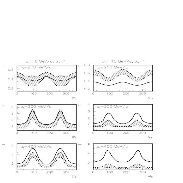
FIG. 7.: The $\phi_{s}$ dependence of $T$ at $p_{t}=0.2~{}GeV/c$, $p_{t}=0.3~{}GeV/c$ and $p_{t}=0.4~{}GeV/c$ and $\alpha_{s}=1$. The solid line is the elastic eikonal approximation. The shaded area presents $T$ including CT within QDM. The parameter $\Delta M^{2}$ lies in the range $0.7-1.1~{}GeV^{2}$.

FIG. 8.: $T$ as a function of projectile momentum $p_{1}$, at $p_{t}=0.2~{}GeV/c$ and $p_{t}=0.4~{}GeV/c$. The solid line is the elastic eikonal approximation. The shaded area presents $T$ including QDM prediction of CT within quantum diffusion model with the parameter $\Delta M^{2}$ within the range $0.7-1.1~{}GeV^{2}$. Dash-doted line - QDM prediction with $\Delta M^{2}=0.7~{}GeV^{2}$, dotted line - $\Delta M^{2}=1.1~{}GeV^{2}$. Dashed line corresponds to prediction CT within the model which accounts for interference between large and small size configurations in $pp$ hard scattering amplitude.

FIG. 9.: The $p_{1}$ dependence of the ratio $R={\sigma(p^{(1)}_{st}\over\sigma(p^{(2)}_{st}}$ at $\alpha_{s}=1$. The solid line is the elastic eikonal approximation. The shaded area is the the $R$ calculated within quantum diffusion model of CT with $\Delta M^{2}$ parameter in the range $0.7-1.1~{}GeV^{2}$. The definitions of curves are same as in Fig.8

FIG. 10.: The ratio $R={\sigma(\phi_{s}={\pi\over 2})\over\sigma(\phi_{s}=\pi)}$ at $\alpha_{s}=1$ as a function of the spectator azimuthal angle $\phi_{s}$ The solid line is the elastic eikonal approximation. The shaded area includes CT, calculated in the QDM, with $\Delta M^{2}$ parameter in the range $0.7-1.1~{}GeV^{2}$.

.

FIG. 11.: The energy dependence of the ratio of the cross sections for the reactions $d(p,2p)n$ and $d(p,2p)N^{*}$. The calculation was done for the elastic eikonal approximation (dashed line) and within the QDM model of CT (solid line), with $\Delta M^{2}=0.7$ GeV².

FIG. 12.: $T$ as a function of $\alpha_{s}$ for different $p_{t}$. The solid lines is for the complete factorization, the dashed and dash-dotted lines are the two calculations which do not have the factorization as explained in Appendix B.

REFERENCES

• [1] L.Β L.Β Frankfurt, E.Β Piasetsky, M.Β M.Β Sargsyan and M.I.Strikman, Phys. Rev. C51, 890 (1995).
• [2] L.Β L.Β Frankfurt, W.Β R.Β Greenberg, G.Β A.Β Miller, M.Β M.Β Sargsyan and M.Β I.Β Strikman, Z.Phys A352 97 (1995).
• [3] L.Β L.Β Frankfurt, G.Β A.Β Miller and M.Β I.Β Strikman, Ann. Rev. of Nuclear and Particle Phys. 44, 501 (1994).
• [4] R.Β J.Β Glauber Phys.Rev. 100, 242 (1955); Lectures in Theoretical Physics, v.1, ed. W.Β Brittain and L.Β G.Β Dunham, Interscience Publ., N.Y. 1959.
• [5] A.Β S.Β Carroll et al., Phys.Rev. Lett. 61, 1698 (1988).
• [6] J.Β P.Β Ralston and B.Β Pire. Phys. Rev. Lett. 61, 1823 (1988)
• [7] B.Β K.Β Jennings and G.Β A.Β Miller Phys. Lett. B318, 7 (1993).
• [8] S.Β J.Β Brodsky, G.Β F.Β De Teramond Phys. Rev. Lett. 60, 1924 (1988).
• [9] A.Β S.Β Caroll et al., BNL Experiment, 850.
• [10] G.Β R.Β Farrar, L.Β L.Β Frankfurt, MΒ .I.Β Strikman andΒ H.Β Liu, Phys Rev Lett. 61, 686 (1988).
• [11] L.Β L.Β Frankfurt, G.Β A.Β Miller, G.Β R.Β Greenberg, and M.Β I.Β Strikman Phys. Rev. C46, 2547 (1992).
• [12] M.Β Lacombe et al., Phys. Rev. C21, 861 (1980).
• [13] R.Β Machleidt K.Β Holinde and C.Β Elster, Phys. Rep. 149, 1 (1987).
• [14] J.Β M.Β Eisenberg Ann. of Physics 71 542 (1972).
• [15] V.Β N.Β Gribov, JETP, 30, 709 (1970).
• [16] L.Β Bertuchi and A.Β Capella Il Nuovo Cimento, A51, 369 (1967).
• [17] L.Β Bertuchi, Il Nuovo Cimento, A11,45 (1972).
• [18] G.Β E.Β Brown and A.D.Β Β Jackson ”The Nucleon-nucleon interaction” North-Holand Publsih. Comp. 1976.
• [19] L.Β L.Β Frankfurt, M.Β M.Β Sargsyan and M.Β I.Β Strikman TAUP-2328-96, nucl-th/9603018, 25pp.
• [20] B.Β K.Β Jennings and G.Β A.Β Miller Phys. Lett. B318, 7 (1993).
• [21] L.Β L.Β Frankfurt, G.Β A.Β Miller and M.Β I.Β Strikman, Comments on nuclear and particle physics, 44, 501 (1993).
• [22] S.Β J.Β Brodsky, in Proceedings if Seventeenth Rencontre de Moriond, ed. J.Β Tran Thanh Van, Editions Frontieres, Gif-sur-Yvette, France, 1982, p.13.
• [23] A.Β H.Β Mueller, in Proceedings if Thirteenth Intl. Symposium on multiparticle Dynamics, ed W.Β Kittel, W.Β Metzegar and A.Β Stergioum World Scientific, SIngapore, 1982, p.963.
• [24] Review of Particle Properties, Phys. Rev. D45 (1992).
• [25] K.Β Sh.Β Egiyan, L.Β L.Β Frankfurt, G.Β A.Β Miller, G.Β R.Β Greenberg, M.Β M.Β Sargsyan and M.Β I.Β Strikman Nucl. Phys. A580, 365 (1994).
• [26] B.Β K.Β Jennings and G.Β A.Β Miller, Phys. Lett. B274, 442 (1992).
• [27] L.Β L.Β Frankfurt, W.Β R.Β Greenberg, G.Β A.Β Miller, M.Β M.Β Sargsyan and M.Β I.Β Strikman, Phys. Lett. B369, 201 (1996).
• [28] S.Β J.Β Brodsky, in Proceedings of AIP Conf. Stony Brook - 1973, 275p.
Refer to caption