PURD-TH-96-05

CERN-TH/96-167

hep-ph/9607386

July 1996

Melting of the Higgs Vacuum:
Conserved Numbers at High Temperature

S. Yu. Khlebnikov${}^{~{}\rm a,}$ and M. E. Shaposhnikov${}^{~{}\rm b,}$

^a Department of Physics, Purdue University, West Lafayette, IN 47907, USA

^b Theory Division, CERN, CH-1211 Geneva 23, Switzerland

Abstract

We discuss the computation of the grand canonical partition sum describing hot matter in systems with the Higgs mechanism in the presence of non-zero conserved global charges. We formulate a set of simple rules for that computation in the high-temperature approximation in the limit of small chemical potentials. As an illustration of the use of these rules, we calculate the leading term in the free energy of the standard model as a function of baryon number B. We show that this quantity depends continuously on the Higgs expectation value $\phi$, with a crossover at $\phi\sim T$ where Debye screening overtakes the Higgs mechanism—the Higgs vacuum “melts”. A number of confusions that exist in the literature regarding the B dependence of the free energy is clarified.

PURD-TH-96-05
CERN-TH/96-167
July 1996

Screening of gauge fields by the Higgs mechanism is one of the central ideas both in modern particle physics and in condensed matter physics. It is often referred to as “spontaneous breaking” of a gauge symmetry, although, in the accurate sense of the word, gauge symmetries cannot be broken in the same way as global ones can. One might rather say that gauge charges are “hidden” by the Higgs mechanism. For example, in the standard model at zero temperature, particles are characterized by values of the electric charge, but not the isospin and the weak hypercharge separately.

At high temperatures, another mechanism for screening becomes operative—the Debye screening of charges in plasma. The Debye screening is not associated with “breaking” or hiding of gauge charges; on the contrary, it is due to the motion of conserved charges. Thus, in the standard model, while all elementary excitations (particles) at zero temperature $(T=0)$ have only one conserved gauge charge with respect to electroweak interactions, it could be different for excitations at $T\not=0$.

In general, we can envisage a competition between the two screening mechanisms. The mass of vector bosons generated by the Higgs mechanism is of order $g\phi$, where $g$ is the gauge coupling and $\phi$ is the temperature dependent Higgs expectation value. The electric mass due to the Debye screening is of order $gT$. So, when $T\ll\phi$, we expect the vacuum classification of particles to be more or less intact; when $T\gg\phi$, the system forgets that the gauge symmetry is “broken”.

At $T\sim\phi$ a crossover occurs, which can be called a melting of the Higgs vacuum. This regime may or may not be associated with a phase transition. A gauge theory may have no gauge-invariant order parameter, and in that case a phase transition does not have to occur [1, 2]. In fact, it was recently shown that the electroweak phase transition changes into a smooth crossover when the mass of the Higgs boson becomes sufficiently large [3]. In this sense, the minimal standard model is similar to the liquid-gas system: there is no true distinction between the phases, and the line of first-order phase transitions ends in a critical point.

The melting of vacuum, associated with a crossover from one screening mechanism to the other, admits a fully gauge-invariant characterization using the renormalized average of $\varphi^{\dagger}\varphi$, where $\varphi$ is the corresponding Higgs field. In the extreme high-temperature limit, in a weakly coupled theory,

$$\langle\varphi^{\dagger}\varphi\rangle_{R}=\nu\frac{T^{2}}{12}+{\rm(corrections)},$$ (1)

where $\nu$ is the number of components of $\varphi$, and the corrections are due to interactions. As the temperature lowers, the leading term starts to deviate from $\nu T^{2}/12$ (at zero temperature it is $v^{2}/2$). Temperatures at which the deviation becomes significant (of the order of the leading term itself) mark the melting crossover.

The above considerations show that the couplings of elementary excitations to gauge fields (the charges) at high temperature can be different from those at $T=0$. This effect can enter calculations of thermodynamic quantities in systems with the Higgs mechanism, which contain, in addition, densities of some conserved global charges. Therefore, a treatment of such systems requires some care. As we will see below, the use of kinetic equilibrium requirements in terms of zero-temperature particle excitations, sometimes invoked [4, 5, 6] in these circumstances, may, and in fact does, lead to wrong results at $\phi~{}\raise 1.29167pt\hbox{$<$\kern-7.5pt\raise-4.73611pt\hbox{$\sim$}}~{}T$.

Although the only application we discuss here will be for the electroweak sector, it is of some interest to sketch a general formalism that would allow one to deal with any case when both the Higgs and the Debye screening mechanisms are present.

In general, a system will have a number of conserved global charges, which we denote by $N_{i}$. These are gauge-invariant quantities that allow for the introduction of chemical potentials, $\mu_{i}$, in the usual way. We thus can define a gauge-invariant grand partition sum as a Euclidean functional integral:

$$\exp(-\Omega/T)=\int{\cal D}\Phi\exp\left[-\int d\tau d^{3}x(L_{E}-\sum\mu_{i}N_{i})\right],$$ (2)

where $\Phi$ denotes generically all of the fields of our system; the integral over $\tau$ is restricted to the finite interval from 0 to $\beta=1/T$, with the usual periodic (antiperiodic) conditions for bosons (fermions). The Lagrangian $L_{E}$ includes gauge-fixing terms and ghosts. The thermodynamic potential $\Omega$ is a gauge-invariant function of $\mu_{i}$ and $T$.

Special attention should be paid to integrals over the Euclidean temporal components of the gauge fields. The integration over their zero-momentum modes, the set of which will be denoted by ${\cal A}_{4}$, enforces the conditions of neutrality of our system with respect to all gauge charges. These conditions are simply a consequence of the Gauss constraint, integrated over the whole three-dimensional (3d) space.

It is convenient to imagine that the functional integration in (2) is performed in two steps. In the first step, we integrate out all modes except for ${\cal A}_{4}$ and the Higgs fields $\varphi$. Those are integrated out at the second step. The reason for this two-step procedure is that ${\cal A}_{4}$ and $\varphi$ can develop expectation values, which we have to take into account. Notice that this general method of calculation of ${\tilde{\Omega}}$ makes no use of the notion of a particle or an elementary excitation in plasma.

The result of the first step is an effective Euclidean action ${\tilde{\Omega}}$

$$\exp(-{\tilde{\Omega}}/T)={\int}^{\prime}{\cal D}\Phi\exp\left[-\int d\tau d^{3}x(L_{E}-\sum\mu_{i}N_{i})\right],$$ (3)

where the prime on the integral shows that the ${\cal A}_{4}$ and $\varphi$ integrations are omitted. ${\tilde{\Omega}}$ is a function of $\mu_{i}$, $T$, ${\cal A}_{4}$ and $\varphi$. One may notice that $i{\cal A}_{4}$ play the role of chemical potentials for the corresponding gauge charges. In general, ${\tilde{\Omega}}$ is a gauge non-invariant quantity; the integration over ${\cal A}_{4}$ and $\varphi$ will convert it into the gauge-invariant potential $\Omega$.

Let us now restrict ourselves to weakly-interacting cases when we can compute ${\tilde{\Omega}}$ by the loop expansion. We will also assume that the expectations values of ${\cal A}_{4}$ and $\varphi$ can be chosen $x$- and $\tau$- independent. The calculation can be done in any desired order; here we will need only tree and one-loop terms. At the tree level, the effective action is the sum of the covariant derivative term for $\varphi$ and its tree potential,

$${\tilde{\Omega}}_{0}/{\cal V}=|D_{4}\varphi|^{2}+V_{0}(\varphi),$$ (4)

where in the covariant derivative we set $\partial_{4}\varphi=0$; ${\cal V}$ is the total 3d volume. One-loop terms can be classified according to powers of ${\cal A}_{4}$. Terms independent of ${\cal A}_{4}$ add to $V_{0}$ to produce the usual temperature-dependent potential for the scalar field. Then, there are linear terms (tadpoles, see Fig. 1), quadratic terms (Debye masses) as well as higher powers. We will assume that the chemical potentials for the global charges are small, $\mu_{i}/T\ll 1$. In that case, the expectation values of ${\cal A}_{4}$ are proportional to $\mu_{i}$, and the terms beyond the quadratic ones are suppressed. In addition, the tadpoles and the Debye masses can be expanded in $\mu_{i}/T$. For the tadpoles, the expansion starts with terms linear in $\mu_{i}$, and for the Debye masses we can, in the leading order, neglect $\mu_{i}$ altogether.

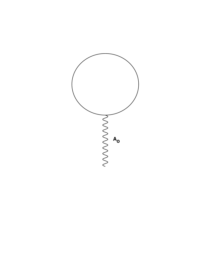
Figure 1: Tadpole diagram producing terms linear in chemical potential.

A particularly simple set of rules arises in the important case when, in addition to the above limits, the masses of all particles are much smaller than $T$. Here the results can be simply formulated using the spectrum of the high-temperature, “unbroken” phase. In that case, the one-loop effective action is obtained as follows. To each particle species of the high-temperature limit we associate a chemical potential

$$\mu_{I}=\sum_{i}\mu_{i}n_{i}^{I}+i\sum_{j}g_{j}^{I}{\cal A}_{4}^{j},$$ (5)

where $n_{i}^{I}$ are the global charges of that species and $g_{j}$ its gauge charges; $I$ labels the species. Note that only ${\cal A}_{4}$, corresponding to the mutually commuting generators of the gauge group, should be taken into account. These generators can be simultaneously diagonalized, and their eigenvalues define what we mean by the charges $g_{j}^{I}$ in eq. (5). The leading terms in the one-loop effective action are

$${\tilde{\Omega}}_{1}/{\cal V}=\left[V_{T}(\varphi)-V_{0}(\varphi)\right]-T^{2}\sum_{I}\eta_{I}\mu_{I}^{2}$$ (6)

where $\eta_{I}=1/6$ ($\eta_{I}=1/12$) per single helicity bosonic (fermionic) particle-antiparticle pair. The complete effective action needed for our purposes is the sum of the tree action (4) and the one-loop action (6).

As an illustration of the use of these rules, we present here a calculation of the leading term in the free energy of the standard model (SM) as a function of the baryon number. It generalizes a similar calculation done in ref. [9], where the only fermionic degrees of freedom were the leptons of the first generation. The B-dependent part of free energy plays an important role in the theory of anomalous electroweak B non-conservation. In our previous calculation of this quantity [7], we pointed out that at sufficiently high temperatures, one may have to use the spectrum of the “unbroken” phase even below the phase transition. Here we extend our previous result and present the leading term in $F(B)$ for all temperatures $T\gg m_{W}(T)$. In particular, we demonstrate a crossover in $F(B)$ at $T\sim\phi$.

As is well known, there are $n_{f}$ strictly conserved global charges in the SM with massless neutrinos, namely

$$N_{i}=\frac{1}{n_{f}}B-L_{i},$$ (7)

where $i=1,...,n_{f}$ is the index of fermionic generation. In addition to them, there are two gauge charges associated with the underlying SU(2)$\times$U(1) symmetry, which commute with the Hamiltonian, the global charges defined by eq. (7), and each other. These are the hypercharge $Y$,

$$Y=i\varphi^{\dagger}\stackrel{{\scriptstyle\leftrightarrow}}{{D}}_{0}\varphi+\sum_{i=1}^{n_{f}}\left[\frac{1}{3}\bar{Q_{i}}\gamma_{0}Q_{i}+\frac{4}{3}\bar{U_{i}}\gamma_{0}U_{i}-\frac{2}{3}\bar{D_{i}}\gamma_{0}D_{i}-\bar{L_{i}}\gamma_{0}L_{i}-2\bar{E_{i}}\gamma_{0}E_{i}\right]$$ (8)

and the third component of the weak isospin $T_{3}$,

$$T_{a}=\epsilon_{abc}A^{b}_{i}G^{c}_{i0}+\frac{1}{2}i\varphi^{\dagger}(\tau^{a}D_{0}-\stackrel{{\scriptstyle\leftarrow}}{{D}}_{0}\tau^{a})\varphi+\frac{1}{2}\sum_{i=1}^{n_{f}}\left[\bar{Q_{i}}\gamma_{0}\tau^{a}Q_{i}+\bar{L_{i}}\gamma_{0}\tau^{a}L_{i}\right].$$ (9)

Here $Q_{i}$ and $L_{i}$ are the left quark and lepton doublets, respectively; $U_{i},~{}D_{i}$ are the right quark fields, and $E_{i}$ are the right leptons.

According to our general rules, we have to introduce $n_{f}$ chemical potentials $\mu_{i}$ to conserved numbers (7), and compute the effective action ${\tilde{\Omega}}(A_{4}^{3},B_{4},\mu_{i},\phi)$, where $\varphi^{T}=(0,\frac{\phi}{\sqrt{2}})$. To make the equations somewhat more transparent we assume here that the asymmetries in charges $N_{i}$ are degenerate in flavour. This assumption is harmless for the leading-order calculation. It would be inadequate if we wanted to include corrections in leptonic masses, which are important in some cosmological scenarios [7]. This assumption sets all $\mu_{i}$ equal to each other and thus replaces them with a single chemical potential for $B-L$. For future purposes, though, we will keep separate chemical potentials for $B$ and $L$. The condition of equilibrium with respect to the anomalous B-non-conservation, $\mu_{B}+\mu_{L}=0$, can be imposed later.

The leading one-loop terms of the high-temperature expansion of the effective action, for small chemical potentials, are

$${\tilde{\Omega}}(A_{4}^{3},B_{4},\mu_{i},\phi)=\frac{1}{2}m^{2}(T)\phi^{2}+\frac{1}{4}\lambda\phi^{4}+$$

$$\frac{1}{8}\phi^{2}(gA_{4}^{3}-g^{\prime}B_{4})^{2}+\frac{1}{2}m_{D}^{2}A_{4}^{3}A_{4}^{3}+\frac{1}{2}m_{D}^{\prime 2}B_{4}B_{4}$$ (10)

$$-\frac{1}{4}n_{f}\mu_{L}^{2}T^{2}-\frac{1}{9}n_{f}\mu_{B}^{2}T^{2}+ig^{\prime}B_{4}n_{f}(\frac{1}{3}\mu_{L}-\frac{1}{9}\mu_{B})T^{2},$$

where

$$m_{D}^{\prime 2} = \biggl{(}\frac{n_{s}}{6}+\frac{5n_{f}}{9}\biggr{)}g^{\prime 2}T^{2},$$ (11)

$$m_{D}^{2} = \biggl{(}\frac{2}{3}+\frac{n_{s}}{6}+\frac{n_{f}}{3}\biggr{)}g^{2}T^{2},$$ (12)

$$m^{2}(T) = -\frac{1}{2}m_{H}^{2}+T^{2}\biggl{(}\frac{1}{2}\lambda+\frac{3}{16}g^{2}+\frac{1}{16}g^{\prime 2}+\frac{1}{4}g_{t}^{2}\biggr{)}.$$ (13)

and $g_{t}$ is the Yukawa coupling of $t$-quark. Terms proportional to $\mu_{B}^{2},\mu_{L}^{2}$ are the standard contributions of the fermionic chemical potentials to $\Omega$, while the terms linear in chemical potential come from the tadpole diagrams of Fig. 1.

The equation (10) forms a basis for determining the equilibrium properties of the hot and dense electroweak plasma at small chemical potentials. As a first example, let us find the equilibrium value $B_{0}$ of the baryonic number at fixed value of the strictly conserved charge $B-L\equiv X$. That equilibrium value is obtained from the solution of the system of equations:

$$\frac{\partial{\tilde{\Omega}}}{\partial A_{4}^{3}}=\frac{\partial{\tilde{\Omega}}}{\partial B_{4}}=0,$$ (14)

(neutrality of the system with respect to gauge charges);

$$-\frac{\partial{\tilde{\Omega}}}{\partial\mu_{B}}=B,{}~{}~{}~{}~{}~{}-\frac{\partial{\tilde{\Omega}}}{\partial\mu_{L}}=L$$ (15)

(definitions of average baryonic and leptonic charges); the equilibrium condition

$$\mu_{B}+\mu_{L}=0,$$ (16)

and the normalization condition $B-L=X$. We get

$$B_{0}=\frac{4(2n_{f}+n_{s})m_{D}^{2}+8(2+2n_{f}+n_{s})m_{W}^{2}(\phi)}{(22n_{f}+13n_{s})m_{D}^{2}+2(26+24n_{f}+13n_{s})m_{W}^{2}(\phi)}(B-L)\;,$$ (17)

where $m_{W}(\phi)=\frac{1}{2}g\phi$. Even if there is a phase transition between the symmetric and Higgs phases, in the Higgs phase with $\phi\ll T$ (the Debye mass is much larger than the Higgs-induced vector mass), we still get the same result as in the symmetric phase [7]

$$B_{0}=\frac{4(2n_{f}+n_{s})}{22n_{f}+13n_{s}}(B-L)\;.$$ (18)

In the opposite limit $\phi\gg T$ we get

$$B_{0}=\frac{4(2+2n_{f}+n_{s})}{26+24n_{f}+13n_{s}}(B-L)\;,$$ (19)

which coincides with the result of refs. [4, 5, 6, 8]. In the intermediate region, the value of the baryon number interpolates between the two limiting cases, see Fig. 2.

Figure 2: Dependence of the equilibrium value of the baryon number (in units of $B-L$) on the expectation value of the Higgs field (in units of temperature) for $n_{f}=3,~{}n_{s}=1$.

For cosmological applications, the relation between $B_{0}$ and $X$ should be taken at the moment of the freeze-out of the sphaleron processes. For a strongly first-order phase transition, when after the transition $\phi/T>$1.2–1.5, the freeze-out coincides with the transition itself, and to a good accuracy one can use the result for the symmetric phase, eq. (18). For a weakly first-order transition, a second-order transition, or a crossover, one should use the full eq. (17) with $\phi/T\simeq 1.2$–$1.5$. (That corresponds to $m_{W}^{2}(\phi)/m_{D}^{2}\simeq 0.2$–$0.3$.) Looking at Fig. 2, we see that for these values of $\phi/T$, the equilibrium value of $B$ is approximately in the middle between its two limiting values.

Although the numerical difference between the limiting values is small, we believe that this calculation is worth-while because it elucidates the physics responsible for the crossover between the high- and low- temperature regimes. What matters here is the relation between $\phi$ and $T$, and not $T$ and $T_{c}$, as stated in refs. [4, 6], or $T$ and $m_{W}(\phi)$ as stated in ref. [7]. The error of the equilibrium reaction analysis of refs. [4, 5, 6] is in the use of the zero-temperature spectrum at high temperatures, which led the authors of these references to conclude that the chemical potential of the Higgs boson is equal to zero. In our notation, that would correspond to $g^{\prime}B_{4}-gA_{4}^{3}=0$. As can be seen directly from eq. (14) with the effective action (10), this condition indeed holds at $T=0$, but not at any $T\neq 0$.

Figure 3: Dependence of the coefficient $\kappa$ on the expectation value of the Higgs field (in units of temperature) for $n_{f}=3,~{}n_{s}=1$.

Another quantity of interest is the free energy of the system at fixed baryonic number $B$, not equal to $B_{0}$, which is used in the computation of the baryon erasure rate due to sphalerons [7]. It is defined as

$$F(B)=\Omega+\mu_{B}B+\mu_{L}L,$$ (20)

where baryonic and leptonic chemical potentials are to be found from eqs. (14,15) but the equilibrium condition (16) is now not imposed. The result is

$$F(B)=\kappa({\phi\over T})\frac{(B-B_{0})^{2}}{{\cal V}T^{2}}+\rm{const},$$ (21)

where

$$\kappa({\phi\over T})=\frac{3[(22n_{f}+13n_{s})m_{D}^{2}+2(26+24n_{f}+13n_{s})m_{W}^{2}(\phi)]}{4n_{f}[(5n_{f}+3n_{s})m_{D}^{2}+(12+11n_{f}+6n_{s})m_{W}^{2}(\phi)]}$$ (22)

For small $\phi/T$ we have

$$\kappa=\frac{3(22n_{f}+13n_{s})}{4n_{f}(5n_{f}+3n_{s})},$$ (23)

which for $n_{s}=1$ coincides with eq. (4.23) of [7]. For large $\phi/T$:

$$\kappa=\frac{3(26+24n_{f}+13n_{s})}{2n_{f}(12+11n_{f}+6n_{s})}$$ (24)

The dependence of $\kappa$ on $\phi/T$ is shown in Fig. 3.

In conclusion, we have presented a general way of dealing with conserved global quantum numbers in finite-temperature gauge theories with the Higgs mechanism. We have formulated a simple set of rules for computing the grand canonical partition sum in the high-temperature limit. Using these techniques, we have computed the leading term of the high-temperature expansion of the free energy of the standard model, as a function of baryon number. We have shown that this quantity depends continuously on the Higgs expectation value $\phi$. The crossover in the free energy is associated with a “melting” of the Higgs vacuum at $\phi\sim T$, when the Debye screening overtakes the Higgs mechanism.

S.K. thanks CERN Theory Division, where part of this work was done, for hospitality. The work of S.K. was supported in part by the U.S. Department of Energy under grant DE-FG02-91ER40681 (Task B), by the National Science Foundation under grant PHY 95-01458, and by the Alfred P. Sloan Foundation.

References

- [1] E. Fradkin and S.H. Shenker. Phys. Rev., D19:3682, 1979.
- [2] T. Banks and E. Rabinovici. Nucl. Phys., B160:349, 1979.
- [3] K. Kajantie, M. Laine, K. Rummukainen, and M. Shaposhnikov. hep-ph/9605288, 1996 and paper in preparation.
- [4] J.A. Harvey and M.S. Turner. Phys. Rev., D42:3344, 1990.
- [5] A.D. Dolgov. Physics Reports, 222:309, 1992.
- [6] H. Dreiner and G.G. Ross. Nucl. Phys., B410:188, 1993.
- [7] S.Yu. Khlebnikov and M.E. Shaposhnikov. Nucl. Phys., B308:885, 1988.
- [8] A.E. Nelson and S.M. Barr. Phys. Lett., B246:141, 1990.
- [9] E.J. Ferrer, V. de la Insera and A.E. Shabad. Nucl. Phys., B309:120, 1988.