RADIATIVE ENERGY LOSS OF HIGH ENERGY QUARKS AND

GLUONS IN A FINITE VOLUME QUARK-GLUON PLASMA

R. Baier ¹, Yu. L. Dokshitzer ², A. H. Mueller ^{3, 4}, S. Peigné ³ and D. Schiff ³

¹Fakultät für Physik, Universität Bielefeld, D-33501 Bielefeld, Germany

² Theory Division, CERN, 1211 Geneva 23, Switzerland

³ LPTHE , Université Paris-Sud, Bâtiment 211, F-91405 Orsay, France

⁴Physics Department, Columbia University, New York, NY 10027, USA

Abstract

The medium induced energy loss spectrum of a high energy quark or gluon traversing a hot QCD medium of finite volume is studied. We model the interaction by a simple picture of static scattering centres. The total induced energy loss is found to grow as $L^{2}$, where $L$ is the extent of the medium. The solution of the energy loss problem is reduced to the solution of a Schrödinger-like equation whose “potential” is given by the single-scattering cross section of the high energy parton in the medium. These results should be directly applicable to a quark-gluon plasma.

1 Introduction

The determination of the radiative energy loss of a high energy charged particle as it passes through matter is a problem studied some time ago, in QED, by Landau, Pomeranchuk and Migdal [1–3]. There is recent data from SLAC [4] on radiative energy loss in QED [5]. New interest in this problem [6–9] has arisen because the corresponding problem in QCD, that of the energy loss of a high energy quark or gluon due to medium stimulated gluon radiation, may be important as a signal for quark-gluon plasma formation in high energy heavy ion collisions.

Recently this problem was considered for infinite matter in [8], hereinafter referred to as BDPS. Using the Gyulassy-Wang (GW) model [6] for hot matter they observed that the QED and QCD problems are mathematically equivalent if one identifies the emission angle of radiated photons in the QED case with the transverse momentum of radiated gluons in the QCD case. The energy loss per unit length, $-\displaystyle{{dE/dz}}$, in hot QCD matter was found to be proportional to $\alpha_{s}\sqrt{E}$ for an incident parton of energy $E$. The $\sqrt{E}$ growth of $-\displaystyle{{dE/dz}}$ was unexpected and suggested that energy losses of high energy jets in a quark-gluon plasma might be large. The procedure used by BDPS was not adequate for determining the exact logarithmic prefactor in $-\displaystyle{{dE/dz}}$. The problem was revisited in [9], hereinafter referred to as BDMPS, where a simple differential equation was given to determine the spectrum $\omega\displaystyle{{dI/d\omega dz}}$ for radiated photons (in QED) and gluons (in QCD) which corrects the prefactor of the result in BDPS.

The present paper generalizes the BDMPS approach to finite length hot matter. Although our discussion is carried out in the context of QCD it is a simple matter to change variables in the QCD results to get the corresponding QED results. Our main interest is in the situation where the incident quark or gluon is sufficiently energetic so that the length of the matter, $L$, satisfies $L<L_{cr}=\sqrt{\lambda_{g}E/\mu^{2}}$, with $\lambda_{g}$ the gluon mean free path and $\mu$ the Debye screening mass of the medium. Our principal results are for $\omega\displaystyle{{dI/d\omega dz}}$, given in (5.16), and for $dE/dz$ given in (6.6) and (6.7). The total energy loss $\Delta E$ in hot QCD matter of length $L$ is $\Delta E=\displaystyle{{\alpha_{s}C_{R}\over 8}}\displaystyle{{\mu^{2}\over\lambda_{g}}}L^{2}\ln(L/\lambda_{g})$ as given in (6.8) with $R$ the colour representation of the incident parton. The total energy loss is found to be proportional to $L^{2}$, a result which is surprising at first glance. However, by considering the limiting case where $L=L_{cr}$ it becomes clear that this corresponds to the BDPS result $\Delta E\propto L_{cr}\sqrt{E}$. The fact that $\Delta E$ is proportional to $L^{2}$ has a simple physical interpretation. Since we expect the energy weighted spectrum $\omega\displaystyle{{dI/d\omega dz}}$ to be integrable in the infrared, $\Delta E$ is roughly determined by the maximum energy a radiated gluon can have still maintaining a coherence length $\leq L$. But, the formation time of a radiated gluon is $\displaystyle{{2\omega/k_{\bot max}^{2}}}$, with $k_{\bot max}$ the maximum transverse momentum that the gluon gets by rescattering in the medium as it is being produced. Taking $k_{\bot max}^{2}=\displaystyle{{L\mu^{2}/\lambda_{g}}}$, with $\mu$ the typical momentum transfer to the gluon in a single scattering, and setting $L\propto\displaystyle{{2\omega\over(L/\lambda_{g})\mu^{2}}}$ one finds $\omega\propto\displaystyle{{1\over 2}}\displaystyle{{\mu^{2}\over\lambda_{g}}}L^{2}$. This estimate, given more precisely in (6.9), leads to the $L^{2}$ dependence of $\Delta E$.

The outline of the paper is as follows:

In section 2 the emission probability of a soft gluon from a high energy quark traversing hot QCD matter is given in the GW model. The basic emission vertex is calculated in detail as are the subsequent rescatterings of the quark-gluon system passing through the matter as the gluon is becoming free. While, for simplicity, much of the discussion is given in the large-$N_{c}$ limit, final formulas are given with exact colour factors. After observing that the QED and QCD emission formulas are identical, with the identification of corresponding variables, the formula for the radiation intensity spectrum $\omega\displaystyle{{dI/d\omega dz}}$ for infinite volume hot QCD matter is given as a direct consequence of the QED spectrum derived by BDMPS.

In section 3 a heuristic discussion of energy loss is given both for $L\ll L_{cr}$ and for $L\gg L_{cr}$. By requiring that these results match at $L_{cr}$ a direct connection between $\Delta E\propto L\sqrt{E}$ for $L\gg L_{cr}$ and $\Delta E\propto L^{2}$ for $L\ll L_{cr}$ is made.

Section 4 is concerned with deriving the general equations governing radiative energy loss in a hot QCD plasma of extent $L$. The basic equation determining energy loss is a Schrödinger-like equation whose “potential” is given in terms of a single scattering cross section, in impact parameter space, of a high energy parton. We expect this same formalism, but with a different “potential”, to apply to the energy loss problem in cold nuclear matter [10]. We presume, however, that the magnitude of the energy loss in hot and cold matter may be quite different.

In section 5 we give an approximate solution for the radiation spectrum valid, at large $L$, for those gluon energies dominating the energy loss of the primary parton. Our main result is given in (5.16). We note that as $L\to\infty$ the spectrum agrees with the result previously given in BDMPS.

Formulas for the total energy loss due to medium induced radiation are given in section 6. We expect the most likely place that these results may have direct phenomenological application is in high energy jet production when a quark-gluon plasma is formed in heavy ion collisions. We also expect results much like (6.6) to hold in jet production in cold nuclear matter, but that is the subject for a subsequent paper [10].

Gluon emission with double scattering is given in Appendix A while rules for dealing with colour factors for multiple scattering are given in Appendix B. The calculation of the planar diagrams necessary to obtain (2.31) is given in Appendix C. A curious integral which arises in evaluating the energy loss is calculated in Appendix D.

2 General expression of the medium induced radiation spectrum in QCD

Here we derive the general form of the gluon energy spectrum induced by the propagation of a high energy quark in a finite non-abelian medium. Results are given for the case of an incident parton of arbitrary colour representation $R$. We also establish a formal analogy between QED and QCD.

2.1 Model for multiple scattering

In order to describe the successive interactions of a high energy incident parton with a hot QCD medium, we use the model introduced by Gyulassy and Wang and recently used in BDMPS to study the photon energy spectrum induced by multiple QED scattering of a fast charged particle. The main feature of the model consists in assuming that scattering centres are static. This allows one to focus on purely radiative processes, since the collisional energy loss then vanishes. The centre located at $\vec{x}_{i}$ creates a screened Coulomb potential

$${\cal V}_{i}(\vec{x})={g\over 4\pi}\ {e^{-\mu|\vec{x}-\vec{x}_{i}|}\over|\vec{x}-\vec{x}_{i}|}\ \ \ ,$$ (2.1)

with Fourier transform

$${\cal V}_{i}(\vec{q})={g\over\vec{q}^{\ 2}+\mu^{2}}\ e^{-i\vec{q}\cdot\vec{x}_{i}}\ \ \ ,$$ (2.2)

where $g$ is the QCD coupling constant. We suppose that the range of the potentials ${\cal V}_{i}$ is small compared to the mean free path $\lambda$ of the incident parton,

$$\mu^{-1}\ll\lambda\ \ \ ,$$ (2.3)

where $\mu$ is the Debye mass induced by the medium. This means that successive scatterings are independent, since the incident parton cannot scatter simultaneously off two distinct centres. As a consequence, its propagation is “time-ordered”, and we may number the scattering centres according to the interaction time (or equivalently the longitudinal coordinate) of the radiating parton. (See [9] for a justification in terms of Feynman diagrams). Moreover, in the context of one gluon emission, this assumption allows us to neglect amplitudes involving four-gluon vertices of the type shown in Fig. 1.

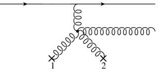
Figure 1: This gluon emission amplitude induced by the scattering of an energetic quark off two static centres 1 and 2 is negligible in the $\lambda\gg\mu^{-1}$ limit.

Finally, we work in the limit of very high energy $E$ for the incident parton and in the soft gluon approximation,

$$\omega\ll E\ \ \ .$$ (2.4)

Let us exhibit the implications of these two assumptions by giving the basic emission amplitude in a single scattering.

2.2 Gluon emission induced by a single scattering

The emission amplitude is depicted in Fig. 2. It includes the emission off the projectile (from now on chosen to be a quark) given by $M_{1}$ and the emission off the exchanged gluon given by $M_{2}$.

$M_{1}=\begin{minipage}[b]{122.85905pt} \centering\includegraphics[width=99.58464pt]{fig2a.ps} \par\vspace{-50pt} \@add@centering\end{minipage}+\begin{minipage}[b]{122.85905pt} \centering\includegraphics[width=99.58464pt]{fig2b.ps} \par\vspace{-50pt} \@add@centering\end{minipage}\ ;\ M_{2}=\begin{minipage}[b]{122.85905pt} \centering\includegraphics[width=99.58464pt]{fig2c.ps} \par\vspace{-50pt} \@add@centering\end{minipage}$

Figure 2: Gluon emission amplitude induced by one scattering.

The colour indices of the static centre and of the incident quark are denoted by $A$, $A^{\prime}$ and $B$, $B^{\prime}$ respectively. The indices of the exchanged and radiated gluons are $a$ and $b$. Neglecting screening for the moment, we write the amplitude for elastic scattering off a static source as

$$M_{e\ell}=T_{B^{\prime}B}^{a}\ M_{A^{\prime}A}^{a}\ \ ;\ \ M_{A^{\prime}A}^{a}=g_{\mu\nu}\ M_{A^{\prime}A}^{a,\mu\nu}\>.$$ (2.5a)

Here

$$M_{A^{\prime}A}^{a,\mu\nu}=ig^{2}(p_{i}+p_{f})^{\mu}{1\over q^{2}}\ \delta_{0}^{\nu}\ T_{A^{\prime}A}^{a}\>,$$ (2.5b)

where we neglected spin effects in the high energy limit. The static source can be viewed as if it were a heavy quark.

In Feynman gauge, the amplitude $M_{1}$ (Fig. 2) for soft gluon emission may be expressed as the elastic scattering amplitude times a radiation factor as

$$M_{1}\simeq-g\left\{{\varepsilon\cdot p_{f}\over k\cdot p_{f}}(T^{b}T^{a})_{B^{\prime}B}-{\varepsilon\cdot p_{i}\over k\cdot p_{i}}(T^{a}T^{b})_{B^{\prime}B}\right\}M_{A^{\prime}A}^{a}\ \ \ ,$$ (2.6)

where $\varepsilon$ denotes the gluon polarization state. The generators of the fundamental representation of $SU(N_{c})$ are $T^{a}(a=1,\ldots N_{c}^{2}-1)$, satisfying $[T^{a},T^{b}]=if^{abc}\ T^{c}$. In the same way we get

$$M_{2}\simeq-g{2\over(p_{f}-p_{i})^{2}}\left\{g_{\mu\nu}\varepsilon\cdot(p_{f}-p_{i})-k_{\mu}\varepsilon_{\nu}+k_{\nu}\varepsilon_{\mu}\right\}\cdot M_{A^{\prime}A}^{a,\mu\nu}\ [T^{b},T^{a}]_{B^{\prime}B}\ .$$ (2.7)

In addition to $M_{1}$ and $M_{2}$, there is a term $M_{3}$ coming from gluon radiation off the static source. The sum of the three terms is gauge invariant. In a physical gauge such as light-cone gauge, $M_{3}$ is down by a factor of $k_{\perp}/\omega$ compared to $M_{1}$ and $M_{2}$. In the calculation given below we use light-cone gauge and assume $k_{\perp}/\omega\ll 1$.

In a hot plasma the source is screened as indicated by (2.1) and (2.2) in the GW model. The reader may have doubts as to the general gauge invariance of that model. These doubts may be put to rest by the following arguments. It is straightforward to show that $M_{1}+M_{2}+M_{3}$ remains gauge invariant when the emitted and exchanged gluons are given the same mass $\mu$. As we shall see later, the emitted gluon has a small impact parameter for the physical problem we consider. As a consequence of the small impact parameter, one may neglect the mass for the emitted gluon; keeping the mass $\mu$ only for the exchanged gluon leads to the Gyulassy-Wang model.

In light-cone gauge

$$\varepsilon=\left(\varepsilon_{0},-\varepsilon_{0},\vec{\varepsilon}_{\bot}\right);\ \varepsilon\cdot k=0\Rightarrow\varepsilon_{0}={\vec{\varepsilon}_{\bot}\cdot\vec{k}_{\bot}\over\omega+k_{//}}\simeq{\vec{\varepsilon}_{\bot}\cdot\vec{k}_{\bot}\over 2\omega}\ .$$ (2.8)

In the high energy limit

$${\varepsilon\cdot p_{i}\over k\cdot p_{i}}\simeq{\varepsilon\cdot p_{f}\over k\cdot p_{f}}\simeq 2\vec{\varepsilon}_{\bot}\cdot{\vec{k}_{\bot}\over k_{\bot}^{2}}\>,$$ (2.9)

where $\vec{k}_{\bot}$ is the transverse momentum of the gluon with respect to the direction of the incident particle. Thus,

$$M_{1}\simeq-2g\ \vec{\varepsilon}_{\bot}\cdot{\vec{k}_{\bot}\over k_{\bot}^{2}}\ [T^{b},T^{a}]_{B^{\prime}B}\ M_{A^{\prime}A}^{a}\ .$$ (2.10)

In QED [9], the photon radiation amplitude vanishes in the limit $E\to\infty$. In QCD, in the high energy limit only the purely non-abelian contribution to the gluon radiation spectrum survives. This is underlined by the presence of the commutator in (2.10). As a result we can use the eikonal approximation where the trajectory of the projectile is taken to be a straight line. Also,

$$M_{2}\simeq 2g\ \vec{\varepsilon}_{\bot}\cdot{\vec{k}_{\bot}-\vec{q}_{\bot}\over(\vec{k}_{\bot}-\vec{q}_{\bot})^{2}}\ [T^{b},T^{a}]_{B^{\prime}B}\ M_{A^{\prime}A}^{a}\ .$$ (2.11)

Finally, the radiation amplitude induced by one scattering of momentum transfer $\vec{q}$ reads

$$M_{1}+M_{2}\simeq-2g\ \vec{\varepsilon}_{\bot}\cdot\vec{J}(k,q)\ [T^{b},T^{a}]_{B^{\prime}B}\ M_{A^{\prime}A}^{a}\ \ \ ,$$ (2.12)

where the emission current $\vec{J}$ is defined as

$$\vec{J}(k,q)={\vec{k}_{\bot}\over k_{\bot}^{2}}-{\vec{k}_{\bot}-\vec{q}_{\bot}\over(\vec{k}_{\bot}-\vec{q}_{\bot})^{2}}\ \ \ .$$ (2.13)

We are interested in the gluon energy spectrum, which is given by the ratio between the radiation and elastic cross sections. Up to a common flux factor

$$d\sigma_{e\ell}\propto C_{F}|M^{a}|^{2}\ dq_{\bot}^{2}\ ;\ C_{F}={N_{c}^{2}-1\over 2N_{c}}\ \ \ ,$$ (2.14a)

$$d\sigma_{rad}\propto{\alpha_{s}\over\pi^{2}}\ C_{F}N_{c}\ \vec{J}^{\,2}\ |M^{a}|^{2}\ d^{2}\vec{k}_{\bot}{dk_{//}\over\omega}dq_{\bot}^{2}\ \ \ ,$$ (2.14b)

where $|M^{a}|^{2}$ is defined as $|M^{a}|^{2}\delta^{a^{\prime}a}=\displaystyle{{1\over N_{c}}}{\rm Tr}\,(M^{a}M^{a^{\prime}})$. Thus we obtain, for $|\vec{k}_{\bot}|\ll\omega\ll E$,

$$\omega{dI\over d\omega d^{2}\vec{k}_{\bot}}=N_{c}\ {\alpha_{s}\over\pi^{2}}\left<\vec{J}(k,q)^{2}\right>\ \ \ .$$ (2.15)

As the amplitude has been evaluated for a fixed momentum transfer $\vec{q}_{\bot}$, an average over $\vec{q}_{\bot}$ has to be performed. For this we use the probability density deduced from the elastic scattering cross section which is easily obtained from (2.2). Thus in (2.15) we define

$$\left<\ (\ \ ...\ \ )\ \right>\>\equiv\>\int d^{2}\vec{q}_{\bot}\ V(q_{\bot}^{2})(\ \ ...\ \ )\>,$$ (2.16)

where the normalized cross section for elastic quark scattering reads

$$V(q_{\bot}^{2})={\mu^{2}\over\pi(q_{\bot}^{2}+\mu^{2})^{2}}\>,$$ (2.17)

with $\int d^{2}\vec{q}_{\bot}\ V(q_{\bot}^{2})=1$. We have used the fact that the longitudinal transfer is negligible with respect to $q_{\bot}$ when $E\to\infty$. As we aim to derive the radiation density induced by multiple scattering, it is convenient to keep the colour structure together with the current and introduce

$$\vec{J}_{eff}=\vec{J}(k,q)\ [T^{b},T^{a}]_{B^{\prime}B}\ \ \ .$$ (2.18)

The fact that the colour structure is the same as the three-gluon vertex allows one to give a compact diagrammatic representation of the effective current as shown in Fig. 3.

$\begin{minipage}[b]{122.85905pt} \centering\includegraphics[width=113.81102pt]{fig3a.ps} \par\vspace{-50pt} \@add@centering\end{minipage}+\begin{minipage}[b]{122.85905pt} \centering\includegraphics[width=113.81102pt]{fig3b.ps} \par\vspace{-50pt} \@add@centering\end{minipage}+\begin{minipage}[b]{122.85905pt} \centering\includegraphics[width=113.81102pt]{fig3c.ps} \par\vspace{-50pt} \@add@centering\end{minipage}$
$\equiv\begin{minipage}[c]{245.71811pt} \centering\includegraphics[width=142.26378pt]{fig3d.ps} \@add@centering\end{minipage}$

Figure 3: Diagrammatic representation of the effective current (2.18).

Then the differential energy spectrum is simply written as

$$\omega{dI\over d\omega\ d^{2}\vec{k}_{\bot}}={\alpha_{s}\over\pi^{2}}\ {\left<|\vec{J}_{eff}|^{2}\right>\over C_{F}\ N_{c}}\ \ \ .$$ (2.19)

A comparison between (2.12) and (2.18) allows one to set the proper colour factor in order to normalize to the elastic scattering cross section. The square $|\vec{J}_{eff}|^{2}$ includes the sum over all colour indices and the $N_{c}$ in the denominator cancels the sum over initial quark colours while $C_{F}$ corresponds to the colour factor of the normalizing elastic cross section. We see that the spectrum (2.19) has exactly the same form as in QED [9], up to the replacement of the photon angle by the gluon transverse momentum (and up to colour factors).

The introduction of the effective current given in (2.18) or in Fig. 3 will provide an important simplification in the case of multiple scattering. Let us indicate how this simplification appears in the case of two scatterings.

2.3 Effective radiation amplitudes for double and multiple scattering

Double scattering.

For two scatterings, the radiation amplitude is given by a collection of seven diagrams. These are simply calculated in the framework of time-ordered perturbation theory. We show in Appendix A that all amplitudes may be grouped in effective radiation amplitudes induced by momentum transfers $\vec{q}_{1}$ or $\vec{q}_{2}$ at times $t_{1}$ and $t_{2}$ ; each is associated with a corresponding phase factor

$$M_{rad}\propto \Big{\{}\vec{J}(k,q_{1})b[c,a]\ e^{it_{1}{k_{\bot}^{2}\over 2\omega}}$$ (2.20)

$$+\vec{J}(k,q_{2})[c,b]a\ e^{it_{2}{k_{\bot}^{2}\over 2\omega}}$$

$$+\vec{J}(k-q_{2},q_{1})[[c,b],a]\ e^{it_{1}{(k-q_{2})_{\bot}^{2}\over 2\omega}+it_{2}{k_{\bot}^{2}-(k-q_{2})_{\bot}^{2}\over 2\omega}}\Big{\}}$$

(see Appendix A for the notation concerning colour factors). This expression multiplies the elastic double scattering amplitude and may be represented diagrammatically as an effective emission current as in Fig. 3. This is shown in Fig. 4.

$M_{rad}\propto\left(\begin{minipage}[c]{98.28574pt} \centering\includegraphics[width=85.35826pt]{fig4a.ps} \@add@centering\end{minipage}\right)\ e^{i\phi_{1}}\ +\left(\begin{minipage}[c]{98.28574pt} \centering\includegraphics[width=85.35826pt]{fig4b.ps} \@add@centering\end{minipage}\right)\ e^{i\phi_{2}}\ +\left(\begin{minipage}[c]{98.28574pt} \centering\includegraphics[width=85.35826pt]{fig4c.ps} \@add@centering\end{minipage}\right)\ e^{i\phi_{12}}$

Figure 4: Radiation amplitude expressed in terms of effective currents.

We thus have

$$M_{rad}\propto\left\{\vec{J}_{eff}(k,q_{1})e^{i\varphi_{{}_{1}}}+\vec{J}_{eff}(k,q_{2})e^{i\varphi_{{}_{2}}}+\vec{J}_{eff}(k-q_{2},q_{1})\ e^{i\varphi_{{}_{12}}}\right\}\ \ \ ,$$ (2.21)

where we use an obvious notation for the phases. The first term on the right-hand side of (2.21) and Fig. 4 corresponds to gluon emission at $t_{1}$ followed by rescattering of the quark at $t_{2}$. The second is gluon production at $t_{2}$ while the third is gluon production at $t_{1}$ followed by rescattering of the gluon at $t_{2}$. As seen from (2.21), quark rescattering does not affect the phase.

Multiple scattering.

The generalization of this simple result to $N$ scatterings is straightforward. After integrating over the time of emission $t$ it is always possible to collect three pieces in order to construct the effective radiation amplitude induced by $\vec{q}_{i}$ at time $t_{i}$. Consider the three light-cone perturbation theory graphs of Fig. 5.

$M_{1}=\begin{minipage}[b]{122.85905pt} \centering\includegraphics[width=99.58464pt]{fig5a.ps} \par\vspace{-30pt} \@add@centering\end{minipage};M_{2}=\begin{minipage}[b]{122.85905pt} \centering\includegraphics[width=99.58464pt]{fig5b.ps} \par\vspace{-30pt} \@add@centering\end{minipage};M_{3}=\begin{minipage}[b]{122.85905pt} \centering\includegraphics[width=99.58464pt]{fig5c.ps} \par\vspace{-30pt} \@add@centering\end{minipage}$

Figure 5: Diagrams contributing to the effective emission amplitude induced by the transfer $\vec{q}_{i\bot}$.

For each diagram, integrating over $t$ yields the difference of two exponential phase factors (see Appendix A). Keeping only the one depending on $t_{i}$, we collect three terms having the same phase,

$${\cal M}_{1}\ \to\ -{\vec{k}_{\bot}\over k_{\bot}^{2}}e^{it_{i}{k_{\bot}^{2}\over 2\omega}}ca_{i}\ \ \ ,$$

$${\cal M}_{2}\ \to\ {\vec{k}_{\bot}\over k_{\bot}^{2}}e^{it_{i}{k_{\bot}^{2}\over 2\omega}}a_{i}c\ \ \ ,$$

$${\cal M}_{3}\ \to\ {\vec{k}_{\bot}-\vec{q}_{i\bot}\over(\vec{k}-\vec{q}_{i})_{\bot}^{2}}e^{it_{i}{k_{\bot}^{2}\over 2\omega}}[c,a_{i}]\ \ \ .$$ (2.22)

The sum of these three terms gives the effective current

$$\vec{J}_{eff}(k,q_{i})=\vec{J}(k,q_{i})[c,a_{i}]=\begin{minipage}[c]{147.43236pt} \centering\includegraphics[width=99.58464pt]{fig6.ps} \par\vspace{0pt} \@add@centering\end{minipage}$$ (2.23)

as in (2.18).

Similarly to the case considered in (2.20), the radiated gluon can rescatter on centres $i\!+\!1,\ldots N$, so that the momentum $k$ and the colour factor have to be changed accordingly in (2.23). For example, if the gluon emitted at centre $i$ rescatters on centre $j$ ($j>i$) the sum of the corresponding three terms results in an expression analogous to (2.22), with $k$ replaced by $(k-q_{j})$, since $k$ labels the final real emitted gluon. In this case, one obtains

$$\vec{J}_{eff}(k-q_{j},q_{i})=\vec{J}(k-q_{j},q_{i})\ a_{N}...a_{j+1}\ a_{j-1}\ldots a_{i+1}[[c,a_{j}],a_{i}]\ .$$ (2.24a)

This is diagrammatically shown below

$$\vec{J}_{eff}(k-q_{j},q_{i})=\begin{minipage}[c]{284.52756pt} {\includegraphics[height=113.81102pt]{fig7.ps}} \end{minipage}$$ (2.24b)

The associated phase is shifted according to

$$\exp\left\{it_{i}{k_{\bot}^{2}\over 2\omega}\right\}\Longrightarrow\exp\left\{it_{i}{(\vec{k}-\vec{q}_{j})_{\bot}^{2}\over 2\omega}+it_{j}{k_{\bot}^{2}-(\vec{k}-\vec{q}_{j})_{\bot}^{2}\over 2\omega}\right\}\ .$$ (2.25)

In the total radiation amplitude, we should include, for centre $i$, the $2^{N-i}$ possibilities (labelled by $i_{r}$) for the quark-gluon system to rescatter on the remaining centres. For $r=1$ to $r=2^{N-i}$, the associated phase gets modified each time the gluon rescatters (the phase is unchanged by quark rescattering). Thus we write

$$M_{rad}\propto\sum_{i=1}^{N}\sum_{r=1}^{2^{N-i}}\vec{J}_{eff}(k_{i_{r}},q_{i})e^{i\varphi_{i_{r}}}\>,$$ (2.26)

where the colour structure is included in $\vec{J}_{eff}$.

2.4 Expression for the radiation spectrum induced by $N$ scatterings

As for a single scattering, we square the radiation amplitude $M_{rad}$ given in (2.26) and normalize by the multiple elastic scattering cross section to get the radiation spectrum induced by $N$ scatterings

$$\omega{dI^{(N)}\over d\omega}={\alpha_{s}\over\pi^{2}}\int d^{2}\vec{k}_{\bot}\left<\sum_{i=1}^{N}\sum_{j=1}^{N}{\vec{J}^{i}_{eff}\cdot\vec{J}^{j\dagger}_{eff}\over N_{c}\ C_{F}^{\ N}}\ e^{i(\varphi_{i}-\varphi_{j})}\right>\>.$$ (2.27)

This expression deserves some comments.

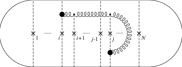
Figure 6: Interference term $\vec{J}^{i}_{eff}\cdot(\vec{J}^{j}_{eff})^{\dagger}$ in the form of a connected graph.

1. In $\vec{J}^{i}_{eff}$, the index $i$ refers to the centre which induces the effective emission current. For a simple calculation of colour factors, it is convenient to represent interference terms in the form of connected diagrams, where the “conjugate amplitude” $(\vec{J}^{j}_{eff})^{\dagger}$ appears in the lower part of the diagram (Fig. 6).

2. The colour factor in the denominator of (2.27) corresponds to the normalization to the elastic scattering cross section, depicted in Fig. 7.

   

   $\ \ =\ N_{c}\ C_{F}^{N}$

   Figure 7: Colour factor associated with the multiple elastic scattering cross section.

   This is easily calculated from the rules given in Appendix B.

3. The sum over all possible gluon rescatterings is implicit in (2.27) (the sum over $r$ in (2.26)). We should take into account all possible ways the quark-gluon system has to rescatter on centres $n$, in particular, for $n\geq j+1$. However this part of the diagram describes the multiple scattering of the produced quark-gluon system after centre $j$, which has no influence on the energy radiation spectrum we are interested in.

4. Between centres $i$ and $j$, it matters whether it is the quark or the gluon which absorbs the transverse momentum $\vec{q}_{n}$, because it changes the relative phase $(\varphi_{i}-\varphi_{j})$. To simplify our derivation, we will first consider the large $N_{c}$ limit, where all non-planar diagrams may be dropped, which corresponds to neglecting quark scatterings on centres $n$ for $i<n<j$.

5. Finally, the brackets in (2.27) denote the average over momentum transfers and longitudinal coordinates of the scattering centres. As in [9] we have

   $$\left<(\ \ ...\ \ )\right>\Leftrightarrow\int\prod_{\ell=1}^{N-1}{d\Delta_{\ell}\over\lambda}\exp\left(-{\Delta_{\ell}\over\lambda}\right)\cdot\int\prod_{i=1}^{N}d^{2}\vec{q}_{i_{\bot}}\ V(q_{i_{\bot}}^{2})(\ \ ...\ \ )\ ,$$ (2.28)

   where $\Delta_{\ell}=z_{\ell+1}-z_{\ell}$ and $V(q_{\bot}^{2})$ is the normalized cross section for elastic scattering, given by (2.17) in the case of Coulomb potentials.

The products $\vec{J}^{i}_{eff}\cdot\vec{J}^{j\dagger}_{eff}$ in (2.27) include a colour sum as indicated in (2.4). We may rewrite (2.27) as

$$\omega{dI^{(N)}\over d\omega}={\alpha_{s}\over\pi^{2}}\int d^{2}\vec{k}_{\bot}\left<2{\rm Re}\sum_{i=1}^{N}\sum_{j=i+1}^{N}{\vec{J}^{i}_{eff}\cdot\vec{J}^{j\dagger}_{eff}\over N_{c}C_{F}^{j-i+1}}\ e^{i(\varphi_{{}_{i}}-\varphi_{{}_{j}})}+\sum_{i=1}^{N}|\vec{J}^{i}_{eff}|^{2}\right>\ .$$ (2.29a)

As in the case of QED [9], we have the equivalent expression

$$\omega{dI^{(N)}\over d\omega}={\alpha_{s}\over\pi^{2}}\int d^{2}\vec{k}_{\bot}\left<2\ {\rm Re}\sum_{i=1}^{N}\sum_{j=i+1}^{N}{\vec{J}^{i}_{eff}\cdot\vec{J}^{j\dagger}_{eff}\over N_{c}\ C_{F}^{j-i+1}}\left(e^{i(\varphi_{{}_{i}}-\varphi_{{}_{j}})}-1\right)+\left|\sum_{i=1}^{N}\vec{J}^{i}_{eff}\right|^{2}\right>\ .$$ (2.29b)

In the large-$N_{c}$ limit $\vec{J}^{i}_{eff}\cdot\vec{J}^{j\dagger}_{eff}$ is given by two sets of planar diagrams denoted by $Y$ and $H$ and shown in (2.4).

$$Y =$$ (2.30a)

$$H =$$ (2.30b)

The second term of (2.29b) is the so-called factorization term, which corresponds to the limit of vanishing phases. In this limit, all emission amplitudes from the internal lines vanish (see Appendix A). Two cases have to be distinguished.

• If the incident quark is produced at a time $t_{0}=-\infty$, we see from Appendix A that only emission amplitudes from initial and final lines remain. The factorization term contribution is then equivalent to the contribution induced by a single scattering of momentum transfer $\vec{q}_{\bot_{tot}}=\sum\limits_{i=1}^{N}\vec{q}_{i}$, and thus has a weak logarithmic medium dependence, as in the QED case [9].

• In a realistic situation where the incident quark is produced, through a hard scattering, at a time $t_{0}=0$, only emission from the final line remains (see the table of Appendix A). In this case the factorization term has no medium dependence at all, so that the medium induced spectrum is exactly given by the first term of (2.29b). It should be directly accessible experimentally by comparing hard scattering on a nucleus with that on a proton.

We show in Appendix C that after dropping the medium-independent factorization term, (2.29b) leads to the following medium-induced radiation spectrum in the large-$N_{c}$ limit

$$\omega{dI^{(N)}\over d\omega}={3\over 2}N_{c}{\alpha_{s}\over\pi^{2}}\int d^{2}\vec{U}\left<2{\rm Re}\sum_{i=1}^{N}\sum_{j=i+1}^{N}\vec{J}_{i}\cdot\vec{J}_{j}\left[\exp\left\{i\kappa\sum_{\ell=i}^{j-1}U_{\ell}^{2}{\Delta_{\ell}\over\lambda}\right\}-1\right]\right>\ ,$$ (2.31)

where the $\vec{U}_{i}$’s are the transverse momenta of the gluon expressed in units of $\mu$,

$$\vec{U}_{i}=\vec{U}_{i-1}-\vec{Q}_{i}$$

$$\vec{U}={\vec{k}_{\bot}\over\mu}\ ;\ \vec{Q}_{i}={\vec{q}_{i}\over\mu}\ ,$$ (2.32)

and $\vec{J}_{i}$ is the rescaled emission current

$$\vec{J}_{i}={\vec{U}_{i}\over U_{i}^{2}}-{\vec{U}_{i-1}\over U_{i-1}^{2}}\ .$$ (2.33)

The dimensionless parameter $\kappa$ is

$$\kappa={\lambda\mu^{2}\over 2}{1\over\omega}\ .$$ (2.34)

The radiation spectrum for the infinite medium QED case was given in [9] for $\kappa\ll 1$. We observe that the expression (2.31) has the same form as in QED [9], with the replacements

$$\alpha\rightarrow{3\over 2}N_{c}\ \alpha_{s}\qquad;\qquad{\omega\over E^{2}}\rightarrow{1\over\omega}\ \ \ ,$$ (2.35a)

$$\hbox{photon ``angle''}\ \vec{U}_{i}\rightarrow\hbox{gluon ``transverse momentum''}\ \vec{U}_{i}\ \ \ .$$ (2.35b)

This analogy allows us to give directly the result for the infinite QCD medium. Thus,

$$\omega{dI\over d\omega dz}={3\alpha_{s}\over 2\pi}\ {N_{c}\over\lambda}\ \sqrt{\kappa\ \ln{1\over\kappa}}\ \ \ .$$ (2.36)

Note that the radiation density is obtained by normalizing (2.31) to the distance $N\lambda$, where $\lambda$ is the mean free path of the incident quark [8].

The changes necessary to include all $\displaystyle{{1\over N_{c}}}$ corrections as well as the case of an arbitrary incident parton of colour represention $R$ have been worked out in [8]. These changes are

$$\kappa \to \widetilde{\kappa}={\widetilde{\lambda}\mu^{2}\over 2}{1\over\omega}\ ;\qquad\widetilde{\lambda}={2C_{F}\lambda\over N_{c}}=2\lambda_{g}\>,$$ (2.37a)

$${N_{c}\over\lambda} \to {N_{c}\over\lambda_{R}}={C_{R}\over\lambda_{g}}\ .$$ (2.37b)

This leads to the general formula

$$\omega{dI\over d\omega dz}={3\alpha_{s}\over 2\pi}{C_{R}\over\lambda_{g}}\sqrt{\widetilde{\kappa}\ln{1\over\widetilde{\kappa}}}={3\alpha_{s}\over 2\pi}\ C_{R}\sqrt{{\mu^{2}\over\lambda_{g}\omega}\ln\left({\omega\over\mu^{2}\lambda_{g}}\right)}\ ,$$ (2.38)

where $\lambda_{g}$ is the gluon mean free path.

We note that apart from the overall normalization, proportional to the squared colour charge $C_{R}$, there is no dependence of the induced radiation spectrum on the nature of the initial parton.

We will now study, for a finite medium, the dependence of the radiation spectrum on the medium size $L=N\lambda$. We present first a heuristic discussion of finite-size effects, and will use (2.31) as a starting point in section 4.

3 Heuristic discussion of the energy loss in finite length media

When a very energetic parton of energy $E$ is propagating through a medium of finite length$L=N\lambda$ the gluon radiation spectrum shows characteristic features depending on the gluon energy $\omega$. For discussing the radiation density $\omega\displaystyle{{dI/d\omega}}$ three different regimes may be distinguished [8,9] : the Bethe-Heitler (BH) regime with small gluon energies, the coherent regime (LPM) for intermediate $\omega$, and the highest energy regime corresponding to the factorization limit. The coherent regime corresponds to the condition (cf. (4.19a) in [9])

$${1\over N^{2}}\ll\kappa\ll 1\ \ \ ,$$ (3.1)

with $\kappa$ given in (2.34) for the QCD case. Thus, for the finite media under consideration a reasonably large number of scatterings will be assumed, $N\gg 1$.

For the following qualitative derivations we neglect logarithmic factors. Thus we ignore numerical factors of order 1, and do not distinguish between propagating quarks and gluons. However we explicitly keep the parameters representing the medium.

In terms of the gluon energy the condition (3.1) is

$$\omega_{BH}\sim\lambda\mu^{2}\ \ll\ \omega\ \ll\ \omega_{fact}\sim{\mu^{2}L^{2}\over\lambda}\leq E\>.$$ (3.2)

Obviously, $\omega_{fact}\leq E$ only holds when $L$ is less than the critical length,

$$L\leq L_{cr}=\sqrt{\frac{\lambda E}{\mu^{2}}}\>.$$ (3.3)

We note that the case $\omega_{fact}\ll E$ is consistent with the soft gluon approximation for the induced spectrum.

The radiation spectrum per unit length behaves in the $E\to\infty$ limit as

$$\omega{dI\over d\omega dz}\simeq\left\{\begin{array}[]{ll}\displaystyle{{\alpha_{s}\over\lambda}}&\qquad\omega<\omega_{BH}\\ \displaystyle{{\alpha_{s}\over\lambda}}\sqrt{\displaystyle{{\lambda\mu^{2}\over\omega}}}&\qquad\omega_{BH}<\omega<\omega_{fact}\\ &\\ \displaystyle{{\alpha_{s}\over L}}&\qquad\omega_{fact}<\omega<E\\ \end{array}\right.$$ (3.4)

for a finite length $L\leq L_{cr}$. These main features are illustrated schematically in Fig. 8. In the BH regime the radiation is due to $N=L/\lambda$ incoherent scatterings, whereas in the factorization regime the medium behaves as one single scattering centre. In the LPM regime $1/\sqrt{\kappa}$ elementary centres act as a single scattering centre.

In order to obtain the total energy loss $\Delta E$ we integrate the spectrum (3.4) over $\omega$ and $z$, with $0\leq\omega\leq E$ and $0\leq z\leq L$. In addition to medium-independent contribution to the energy loss proportional to $\alpha_{s}E$ (a factorization contribution), we find the induced loss

$$\Delta E(L)\sim\alpha_{s}{\mu^{2}L^{2}\over\lambda}\left(1+O\left(\displaystyle{{1\over N}}\right)\right).$$ (3.5)

It has been already pointed out in [11], that the total energy loss increases quadratically with the length $L$, and is independent of the parton energy $E$ in the high energy limit. This interesting case is investigated in more detail in what follows.

Here we conclude this heuristic discussion by considering the case of finite $L$, but with $L>L_{cr}$. This situation occurs for parton energies $E\leq E_{cr}=L^{2}\mu^{2}/\lambda$ (see (3.3)). By extending the coherent soft $\omega$-spectrum (3.4) up to $\omega\sim E$, the total induced loss is

$$\Delta E(L)\>\simeq\>\alpha_{s}\sqrt{{\mu^{2}E\over\lambda}}\,L\>=\>\alpha_{s}\sqrt{E\ E_{cr}}\ \ \ ,$$ (3.6)

which is $E$-dependent and linear in $L$. The results given in (3.5) and (3.6) are schematically summarized in Fig. 9, where the $E$ dependence of $\Delta E$ is plotted for fixed $L$, and in Fig. 10, where $E$ is fixed and the $L$-dependence is shown.

The loss given by (3.6) is also relevant for an infinite medium, $L\to\infty$. An $E$-dependent loss per unit length of propagating partons is found [8],

$$-{dE\over dz}\>\simeq\>\alpha_{s}\sqrt{{\mu^{2}E\over\lambda}}\>.$$ (3.7)

Figure 8: Radiation density (3.4) for a medium of finite length $L<L_{cr}$.

Figure 9: Total induced energy loss as a function of the parton energy $E$.

Figure 10: Total induced energy loss as a function of the medium size $L$.

4 General equation for the induced radiation spectrum

In this section we shall derive the general equations which govern the induced radiation spectrum for finite length materials. These equations generalize (4.34) and (4.40) of BDMPS. Our starting point, for the sake of simplicity, is the large-$N_{c}$ formula (2.31). We divide by $L$, the length of the material, and we allow the sum over scatterings to be arbitrary in number giving

$${\omega\>dI\over d\omega dz}={3\alpha_{s}N_{c}\over 2L\pi^{2}}\int_{0}^{L}d\Delta\int d^{2}\vec{U}\left<2{\rm Re}\sum_{i=1}^{\infty}\sum_{j=i+1}^{\infty}\vec{J}_{i}\cdot\vec{J}_{j}\left[\exp\left\{i\kappa\sum_{\ell=i}^{j-1}U_{\ell}^{2}{\Delta_{\ell}\over\lambda}\right\}-1\right]\delta\left(\Delta-\sum_{m=1}^{\infty}\Delta_{m}\right)\right>,$$ (4.1)

where $\Delta$ is the distance between the first and last scatterings. Expressing the sum over $i$ as an integral of the position in the medium of the gluon emission vertex $\vec{J}_{i}$ and neglecting initial and final state scattering one arrives at

$$\omega{dI\over d\omega dz}={3\alpha_{s}N_{c}\over 2L\pi^{2}}\int_{0}^{L}d\Delta\int_{0}^{L-\Delta}{dz_{1}\over\lambda}\int d^{2}\vec{U}$$

$$\cdot\left<2{\rm Re}\sum_{n=0}^{\infty}\vec{J}_{1}\cdot\vec{J}_{n+2}\left[\exp\left\{i\kappa\sum_{\ell=1}^{n+1}U_{\ell}^{2}{\Delta_{\ell}\over\lambda}\right\}-1\right]\delta\left(\Delta-\sum_{m=1}^{n+1}\Delta_{m}\right)\right>,$$ (4.2)

where now $\Delta$ is the distance between the emission vertices $\vec{J}_{1}$ and $\vec{J}_{n+2}$. Although the sum in (4.2) formally goes from $n=0$ to $n=\infty$ we expect the typical number of scatterings to be $L/\lambda$. It is convenient to scale all distances by the mean free path $\lambda$. To that end let

$$t={\Delta\over\lambda}\quad,\quad t_{\ell}={\Delta_{\ell}\over\lambda}\quad,\quad T={L\over\lambda}\>.$$

Then

$$\omega{dI\over d\omega dz}={3\alpha_{s}N_{c}\over 2\lambda\pi}\int_{0}^{T}dt\>(1-{t\over T})\int{d^{2}\vec{U}\over\pi}2{\rm Re}\sum_{n=0}^{\infty}\int\prod_{\ell=1}^{n+2}d^{2}\vec{Q}_{\ell}V(Q_{\ell}^{2})\vec{J}_{1}\cdot\vec{J}_{n+2}$$

$$\cdot\int\prod_{r=1}^{n+1}e^{-t_{r}}dt_{r}\left[\exp\left\{i\kappa\sum_{s=1}^{n+1}U_{s}^{2}t_{s}\right\}-1\right]\delta\left(t-\sum_{m=1}^{n+1}t_{m}\right),$$ (4.3)

where we have done the integral over $z_{1}$. In (4.3) the dependence on $\vec{Q}_{1}$ and $\vec{Q}_{n+2}$ is contained only in the product of currents

$$\vec{J}_{1}\cdot\vec{J}_{n+2}=\left({\vec{U}_{1}\over U_{1}^{2}}-{\vec{U}_{1}+\vec{Q}_{1}\over(\vec{U}_{1}+\vec{Q}_{1})^{2}}\right)\cdot\left({\vec{U}_{n+1}-\vec{Q}_{n+2}\over(\vec{U}_{n+1}-\vec{Q}_{n+2})^{2}}-{\vec{U}_{n+1}\over U_{n+1}^{2}}\right),$$ (4.4)

and in $V(Q_{1}^{2})$ and $V(Q_{n+2}^{2})$. As in BDMPS we integrate first over $\vec{Q}_{1}$ and $\vec{Q}_{n+2}$ holding $\vec{U}_{1}$, $\vec{U}_{2},\ldots\vec{U}_{n+1}$ fixed. Defining an averaged elementary current

$$\vec{f}_{0}(\vec{U}_{1})\equiv\int d^{2}\vec{Q}_{1}V(Q_{1}^{2})\vec{J}_{1}=\pi{\vec{U}_{1}\over U_{1}^{2}}\int_{U_{1}^{2}}^{\infty}dQ^{2}V(Q^{2})\>,$$ (4.5)

we note that

$$\vec{f}_{0}(\vec{U}_{n+1})=-\int d^{2}\vec{Q}_{n+2}\ V(Q_{n+2}^{2})\ \vec{J}_{n+2}\>.$$ (4.6)

The spectrum can be written as

$$\left.\omega{dI\over d\omega dz}={3\alpha_{s}N_{c}\over 2\pi\lambda}2{\rm Re}\int_{0}^{T}dt\ (1-{t\over T})\int{d^{2}\vec{U}_{1}\over\pi}\vec{f}_{0}(\vec{U}_{1})\cdot\vec{f}(\vec{U}_{1},t)\right|_{\kappa}^{\kappa=0}\>,$$ (4.7)

where

$$\vec{f}(\vec{U}_{1},t)=\vec{f}_{0}(\vec{U}_{1})e^{-t(1-i\kappa U_{1}^{2})}+e^{-t(1-i\kappa U_{1}^{2})}\sum_{n=1}^{\infty}\prod_{\ell=2}^{n+1}\int d^{2}\vec{Q}_{\ell}V(Q_{\ell}^{2})$$

$$\cdot\prod_{r=2}^{n+1}\int dt_{r}\ e^{-i\kappa t_{r}(U_{1}^{2}-U_{r}^{2})}\>\Theta\left(t-\sum_{m=2}^{n+1}t_{m}\right)\vec{f}_{0}(\vec{U}_{n+1})\>.$$ (4.8)

The first term on the right-hand side of (4.8) is the $j=i\!+\!1$ (nearest neighbours, $n\!=\!0$) term of (2.31). The rest of the terms in (4.8) correspond to arbitrary numbers of gluon rescatterings between the currents 1 and $n\!+\!2$.

Equation (4.8) has a Bethe-Salpeter structure so it is straightforward to check that $\vec{f}(\vec{U},t)$ satisfies the natural integral equation

$$\vec{f}(\vec{U},t)=\vec{f}(\vec{U},0)e^{-t(1-i\kappa U^{2})}+\int d^{2}\vec{Q}\ V(Q^{2})\int_{0}^{t}dt^{\prime}\ e^{-(t-t^{\prime})(1-i\kappa U^{2})}\vec{f}(\vec{U}-\vec{Q},t^{\prime}),$$ (4.9)

where

$$\vec{f}(\vec{U},0)\equiv\vec{f}_{0}(\vec{U})\>,$$ (4.10)

and where we have used

$$\vec{U}_{\ell}=\vec{U}_{\ell-1}-\vec{Q}_{\ell}\>.$$ (4.11)

It is convenient to eliminate the $t$-integration on the right-hand side of (4.9). This is achieved by taking a $t$-derivative which gives

$${\partial\over\partial t}\vec{f}(\vec{U},t)=-(1-i\kappa U^{2})\>\vec{f}(\vec{U},t)+\int d^{2}\vec{Q}\ V(Q^{2})\ \vec{f}(\vec{U}-\vec{Q},t)\>.$$ (4.12)

Although (4.12) has been derived for an incident quark in the large-$N_{c}$ limit, essentially the same equation holds for partons of colour representation $R$ even without taking the large-$N_{c}$ limit. In the general case

$$\vec{f}(\vec{U},t_{R}) = {N_{c}\over 2C_{R}}\vec{f}_{0}(\vec{U})\>e^{-t_{R}(1-i\kappa_{R}U^{2})}+{N_{c}\over 2C_{R}}\int\!d^{2}\vec{Q}\,V(Q^{2})\int_{0}^{t_{R}}\!dt^{\prime}_{R}\ e^{-(t_{R}-t^{\prime}_{R})(1-i\kappa_{R}U^{2})}\vec{f}(\vec{U}\!-\!\vec{Q},t^{\prime}_{R})$$ (4.13)

$$+ \left(1-{N_{c}\over 2C_{R}}\right)\int^{t_{R}}_{0}dt^{\prime}_{R}\ e^{-(t_{R}-t^{\prime}_{R})(1-i\kappa_{R}U^{2})}\vec{f}(\vec{U},t^{\prime}_{R})$$

replaces (4.9) with $t_{R}=z/\lambda_{R}$, $\kappa_{R}=\mu^{2}\lambda_{R}/2\omega$ and where $\lambda_{R}=\lambda C_{F}/C_{R}$. The second term on the right-hand side of (4.13) corresponds to the emitted gluon rescattering which is dominant for incident quarks in the large $N_{c}$ limit, and thus corresponds to the second term on the right-hand side of (4.9). The third term on the right-hand side of (4.13) is necessary to generate the non-planar graphs corresponding to the incident parton rescattering in the medium as discussed in BDPS. Indeed, as already discussed in section 2, there is no additional phase factor associated with the incident parton rescattering. As a result, this term is $Q$-independent and we can use $\int d^{2}\vec{Q}\,V(Q^{2})=1$.

The colour factors appearing in (4.13) may be easily obtained from Appendix B. Taking a time derivative on both sides of (4.13), and defining

$$\tau={N_{c}\over 2C_{R}}t_{R}\quad,\quad\tau_{0}={N_{c}\over 2C_{R}}T_{R}\>,$$ (4.14)

$$\widetilde{\kappa}={2C_{R}\over N_{c}}\kappa\>,$$ (4.15)

we find

$${\partial\over\partial\tau}\vec{f}(\vec{U},\tau)=-(1-i\widetilde{\kappa}U^{2})\vec{f}(\vec{U},\tau)+\int d^{2}\vec{Q}\ V(Q^{2})\ \vec{f}(\vec{U}-\vec{Q},\tau)\>,$$ (4.16)

which equation is identical in form to (4.12). It is remarkable that the equation for the spectrum keeps the simple form

$$\left.\omega{dI\over d\omega dz}={3\alpha_{s}C_{R}\over 2\pi\lambda_{g}}2{\rm Re}\int_{0}^{\tau_{0}}d\tau\left(1-{\tau\over\tau_{0}}\right)\int{d^{2}\vec{U}_{1}\over\pi}\vec{f}_{0}(\vec{U}_{1})\cdot\vec{f}(\vec{U}_{1},\tau)\right|_{\tilde{\kappa}}^{\tilde{\kappa}=0}\ \ \ ,$$ (4.17)

provided we take with (4.16) the initial condition

$$\vec{f}(\vec{U},0)=\vec{f}_{0}(\vec{U})\ \ \ ,$$ (4.18)

instead of the initial condition implied in (4.13).

We can make contact with the formalism of BDMPS for infinite length matter by taking $\tau_{0}=\infty$ in (4.17). Identifying

$$\vec{f}(\vec{U})=\int_{0}^{\infty}d\tau\ \vec{f}(\vec{U},\tau)\ \ \ ,$$ (4.19)

we see that (4.17) agrees with (4.28) of BDMPS when account is taken of the replacement $\alpha\to\displaystyle{{3\over 2}}\alpha_{s}N_{c}$ necessary to go from QED to QCD. Integrating (4.16) over $\tau$ between $\tau=0$ and $\tau=\infty$ gives

$$(1-i\widetilde{\kappa}U^{2})\ \vec{f}(\vec{U})=\vec{f}_{0}(\vec{U})+\int d^{2}\vec{Q}\ V(Q^{2})\ \vec{f}(\vec{U}-\vec{Q})\ \ \ ,$$ (4.20)

which again reproduces the BDMPS result given in (4.30).

Just as (4.20) was solved, for small $\widetilde{\kappa}$, by going to impact parameter space, it is convenient to recast (4.16) by defining

$$\widetilde{\vec{f_{\ }}}(\vec{B},\tau)=\int d^{2}\vec{U}\ e^{-i\vec{B}\cdot\vec{U}}\ \vec{f}(\vec{U},\tau)\ \ \ ,$$ (4.21)

$$\widetilde{V}(B^{2})=\int d^{2}\vec{Q}\ e^{-i\vec{B}\cdot\vec{Q}}V(Q^{2})\ \ \ ,$$ (4.22)

which leads to

$${\partial\over\partial\tau}\widetilde{\vec{f_{\ }}}(\vec{B},\tau)=\left[-i\widetilde{\kappa}\nabla_{B}^{2}-(1-\widetilde{V}(B^{2}))\right]\widetilde{\vec{f_{\ }}}(\vec{B},\tau)\ \ \ .$$ (4.23)

We can also use (4.21) to rewrite the spectrum (4.17) as an integral over impact parameter with the result

$$\omega\left.{dI\over d\omega dz}={3\alpha_{s}C_{R}\over 2\pi^{2}\lambda_{g}}2\,{\rm Re}\left\{i\int_{0}^{\tau_{0}}d\tau\left(1-{\tau\over\tau_{0}}\right)\int{d^{2}\vec{B}\over 2\pi}\ {1-\widetilde{V}(B^{2})\over B^{2}}\vec{B}\cdot\widetilde{\vec{f_{\ }}}(\vec{B},\tau)\right|_{\tilde{\kappa}}^{\tilde{\kappa}=0}\right\},$$ (4.24)

the finite length generalization of (4.40) of BDMPS. In arriving at (4.24) we have used

$$\widetilde{\vec{f_{\ }}}_{0}(\vec{B})=-2\pi i{\vec{B}\over B^{2}}(1-\widetilde{V}(B^{2}))\>.$$ (4.25)

Equations (4.23) and (4.24), along with the initial condition $\widetilde{\vec{f_{\ }}}(\vec{B},0)=\widetilde{\vec{f_{\ }}}_{0}(\vec{B})$ are the general equations governing the induced radiation spectrum for finite length matter in the context of the Gyulassy-Wang model of a hot QCD plasma.

5 Solution for the radiation spectrum in the small $\kappa$ limit

In this section we give an approximate solution to (4.23) and (4.24) valid in the small $\kappa$ limit. We restrict our evaluation of (4.24) to $\omega$ values not too far from those which dominate the energy loss in finite length hot matter. The exact region of validity of our approach should become apparent as we proceed.

Eq. (4.23) has a close resemblance to a Schrödinger, or diffusion, equation. However, since the general Schrödinger equation cannot be solved explicitely this analogy is not in itself useful. But, (4.23) is not only close to a Schrödinger equation it is even close to the Schrödinger equation for a two dimensional harmonic oscillator. To see this we recall that in infinite length matter the values of $B$ which dominate the energy loss problem are those where $B^{2}\sim\sqrt{\kappa}$ and we shall later see the same to be true in finite length matter. Also, recall that $1-\widetilde{V}(B^{2})\approx{1\over 4}B^{2}\ln(1/B^{2})$ for small $B$ for Coulomb scattering. At small $B^{2}$, $\ln(1/B^{2})$ varies much more slowly than $B^{2}$ so we may expect a reasonable approximation to consist in neglecting the variation of $\ln(1/B^{2})$ when solving (4.23). In this case (4.23) can be solved in terms of the general solution to the Schrödinger equation for the 2-dimensional harmonic oscillator. In order to discuss the solution to (4.23) in a context somewhat more general than that of Coulomb scattering write this equation as

$$i{\partial\over\partial\tau}\widetilde{\vec{f_{\ }}}(\vec{B},\tau)=\left[\widetilde{\kappa}\nabla_{B}^{2}-i{B^{2}\over 4}\widetilde{v}(B^{2})\right]\widetilde{\vec{f_{\ }}}(\vec{B},\tau)\>;\qquad\widetilde{\vec{f}}(\vec{B},0)=-\frac{i\pi}{2}\vec{B}\,\widetilde{v}(B^{2})\>,$$ (5.1)

where $\widetilde{v}(B^{2})\equiv 4(1-\widetilde{V}(B^{2}))/B^{2}$. For potentials which decrease rapidly at large momentum transfer $\widetilde{v}(B^{2})\approx\widetilde{v}(0)$ at small $B^{2}$ and $\widetilde{v}(0)\mu^{2}$ is just the mean momentum transfer squared. In the Coulomb case, $\widetilde{v}(B^{2})\approx\ln 1/B^{2}$ for small $B^{2}$ . We expect our approach to be valid whenever

$$B^{2}{\partial\over\partial B^{2}}\ln\ \widetilde{v}(B^{2})\ll 1\ \ \ ,$$ (5.2)

for small $B^{2}$. In the Coulomb case we expect our answer for $\omega\displaystyle{{dI/d\omega dz}}$ to be correct within logarithmic accuracy in $1/\kappa$.

So long as $\widetilde{v}(B^{2})$ can be treated as a constant the solution to (4.23) proceeds in analogy with that of the two dimensional harmonic oscillator

$$i{\partial\over\partial t}\psi(\vec{B},t)=\left[-{1\over 2m}\nabla_{B}^{2}+{1\over 2}m\omega_{0}^{2}B^{2}\right]\psi(\vec{B},t)\ \ \ .$$ (5.3)

Comparing (5.1) and (5.3) it is clear that one may take solutions to the harmonic oscillator if the identifications

$$m=-{1\over 2\widetilde{\kappa}}\quad,\quad\omega_{0}=\sqrt{i\widetilde{\kappa}\widetilde{v}}$$ (5.4)

are made. Thus we may immediately write the function $\widetilde{\vec{f_{\ }}}$ in terms of the Green function $G$ as

$$\widetilde{\vec{f_{\ }}}(\vec{B},\tau)=\int d^{2}\vec{B}^{\prime}\ G(\vec{B},\tau;\vec{B}^{\prime},0)\widetilde{\vec{f_{\ }}}(\vec{B}^{\prime},0)\ \ \ ,$$ (5.5)

where

$$G(\vec{B},\tau;\vec{B}^{\prime},0)={m\omega_{0}\over 2\pi i\sin\omega_{0}\tau}\exp\left\{{im\omega_{0}\over 2\sin\omega_{0}\tau}\left[(B^{2}+B^{\prime 2})\cos\omega_{0}\tau-2\vec{B}\cdot\vec{B}^{\prime}\right]\right\}\ \ \ ,$$ (5.6)

with $\omega_{0}$ and $m$ as given in (5.4).

Eq. (5.5) can be written as

$$\widetilde{\vec{f_{\ }}}(\vec{B},\tau)=N\ e^{-\gamma B^{2}}\int d^{2}\vec{B}^{\prime}\ e^{-\alpha(\vec{B}^{\prime}-\vec{C})^{2}}\ \widetilde{\vec{f_{\ }}}(\vec{B}^{\prime},0)\ \ \ ,$$ (5.7)

where

$$\alpha={-im\omega_{0}\over 2\tan\omega_{0}\tau}\quad,\quad\gamma={i\over 2}m\omega_{0}\tan\omega_{0}\tau\quad,\quad\vec{C}={\vec{B}\over\cos\omega_{0}\tau}\quad,\quad N={m\omega_{0}\over 2\pi i\sin\omega_{0}\tau}\ .$$ (5.8)

Using $\sqrt{i}=\displaystyle{{1+i\over\sqrt{2}}}$ one sees that ${\rm Re}\ \alpha>0$ and $|\alpha|\gg 1$ for all values of $\tau$. Indeed for $\tau\ll|\omega_{0}|^{-1}$

$$\alpha\approx{i\over 4\widetilde{\kappa}\tau}+{1\over 12}\widetilde{v}\tau\ \ \ ,$$ (5.9a)

while for $\tau\gg|\omega_{0}|^{-1}$

$$\alpha\approx{1+i\over 4}\sqrt{{\widetilde{v}\over 2\widetilde{\kappa}}}\ \ \ .$$ (5.9b)

Hence $|\alpha|\raise 1.29167pt\hbox{$>$\kern-7.5pt\raise-4.73611pt\hbox{$\sim$}}1/\sqrt{\widetilde{\kappa}}$ for all $\tau$. Thus so long as $\widetilde{\kappa}$ is small the integral in (5.7) is dominated by values of $|\vec{B}^{\prime}-\vec{C}|^{2}$ on the order of $|\alpha|^{-1}\ll 1$. Since we do not expect a rapid variation of $\widetilde{\vec{f_{\ }}}(\vec{B}^{\prime},0)$ with $\vec{B}^{\prime}$, the integral in (5.7) can be done by replacing $\vec{B}^{\prime}$ by $\vec{C}$ in that function and then carrying out the gaussian integration over $\vec{B}^{\prime}$. One finds

$$\widetilde{\vec{f_{\ }}}(\vec{B},\tau)={\pi N\over\alpha}e^{-\gamma B^{2}}\ \widetilde{\vec{f_{\ }}}(\vec{C},0)\ \ \ .$$ (5.10)

As we shall see below we always use values of $\tau$ and $\omega$ for which $\omega_{0}\tau$ is of order 1. Thus from (5.8) it is clear that $\vec{C}$ is of the same order as $\vec{B}$.

Recalling that

$$\widetilde{\vec{f_{\ }}}(\vec{C},0)=\widetilde{\vec{f_{\ }}}_{0}(\vec{C})=-{\pi i\over 2}\vec{C}\widetilde{v}(C^{2})\ \ \ ,$$ (5.11)

we can write

$$\widetilde{\vec{f_{\ }}}(\vec{B},\tau)=-{i\pi\widetilde{v}(B^{2})\vec{B}\over 2\cos^{2}\omega_{0}\tau}\exp\left\{-{i\over 2}m\omega_{0}B^{2}\tan\omega_{0}\tau\right\}\ \ \ ,$$ (5.12)

where we have used the fact that $\widetilde{v}$ is slowly varying to replace $C^{2}$ by $B^{2}$ as the argument of that function. Finally, from the above it is apparent that $\vec{B}^{\prime}$, in (5.7) is comparable to $\vec{B}$. This occurs because the parameter $\widetilde{\kappa}$ in (5.1) is small thus severely limiting the diffusion in $\vec{B}$ so that the time development of $\widetilde{\vec{f_{\ }}}(\vec{B},\tau)$ occurs with only moderate variations of $\vec{B}$. That is, the impact parameter of the produced gluon is effectively frozen (at small values) during the whole time of its production.

We can now use (5.12) in (4.24). The integration over $\tau$ is made simple by noting that

$$\widetilde{\vec{f_{\ }}}(\vec{B},\tau)={2\pi i\vec{B}\over B^{2}}\ {\partial\over\partial\tau}\exp\left\{-{i\over 2}m\omega_{0}B^{2}\tan\omega_{0}\tau\right\}\>.$$ (5.13)

We emphasize that in the case when $\tilde{v}$ is a constant, (5.13) is an exact solution to (5.1).

Substituting (5.13) into (4.24) leads to

$$\left.\omega{dI\over d\omega dz}=-{3\alpha_{s}C_{R}\over 4\pi^{2}\lambda_{g}\tau_{0}}{\rm Re}\int_{0}^{\tau_{0}}d\tau\int\widetilde{v}(B^{2})d^{2}\vec{B}\exp\left\{-{i\over 2}m\omega_{0}B^{2}\tan\omega_{0}\tau\right\}\right|_{\tilde{\kappa}}^{\tilde{\kappa}=0}\ .$$ (5.14)

We now do the $B$-integration, again neglecting the $B$-dependence of $\widetilde{v}$. One finds

$$\omega{dI\over d\omega dz}={3\alpha_{s}C_{R}\over 2\pi\lambda_{g}\tau_{0}}{\rm Re}\int_{0}^{\tau_{0}}d\tau\>2\left[\,\frac{\omega_{0}}{\tan\omega_{0}\tau}-\frac{1}{\tau}\,\right].$$ (5.15)

The $B$-integration in (5.14) is determined by values of $B^{2}$ on the order of $|m\omega_{0}\tan\omega_{0}\tau|^{-1}$. However, as is clear from (5.15) values of $|\omega_{0}\tau|\ll 1$ do not contribute significantly to $\omega\displaystyle{{dI/d\omega dz}}$, so we may assume that $|\omega_{0}\tau|\geq 1$. This means that $B^{2}$ is on the order of $|m\omega_{0}|^{-1}$ which, from (5.4) gives $B^{2}\sim\sqrt{\widetilde{\kappa}/\widetilde{v}(B^{2})}$ as dominanting the spectrum of radiated gluons. In the Coulomb case this means $B^{2}\sim\sqrt{\widetilde{\kappa}/\ln(1/\widetilde{\kappa})}$ while for potentials which decrease rapidly in transverse momentum, $B^{2}\sim\sqrt{\widetilde{\kappa}}$ is dominant.

The time integral in (5.15) is easily performed and gives

$$\omega{dI\over d\omega dz}={6\alpha_{s}C_{R}\over\pi L}\ \ln\left|{\sin(\omega_{0}\tau_{0})\over\omega_{0}\tau_{0}}\right|\>,$$ (5.16)

where we have set $\tau_{0}\widetilde{\lambda}=L$ the length of the matter. The coupling $\alpha_{s}$ in (5.16) should be evaluated at momentum scale on the order of $\mu^{2}/B^{2}=\mu^{2}\sqrt{(\ln\ 1/\widetilde{\kappa})/\widetilde{\kappa}}$. We note that $\omega\displaystyle{{dI/d\omega dz}}$ is small when $|\omega_{0}\tau_{0}|\ll 1$, while

$$\omega{dI\over d\omega dz}\ \mathrel{\mathop{\longrightarrow}_{|\omega_{0}\tau_{0}|\to\infty}}\ {3\alpha_{s}C_{R}\over 2\pi\lambda_{g}}\sqrt{2\widetilde{\kappa}\widetilde{v}(\sqrt{\widetilde{\kappa}})}\ \ \ .$$ (5.17)

In the Coulomb case $\widetilde{v}(\sqrt{\widetilde{\kappa}})={\textstyle{1\over 2}}\ln(1/\widetilde{\kappa})$ bringing (5.17) in agreement with (2.38) and with (5.1) of BDMPS for infinite length matter.

6 Energy loss in a finite length medium

In order to find the total energy loss it is necessary to integrate (5.16) over $\omega$. However, it is technically easier to go back to (5.15) and do the $\omega$-integral before doing the $\tau$-integration. Thus

$$-{dE\over dz}=\int\omega{dI\over d\omega dz}d\omega={3\alpha_{s}C_{R}\over 2\pi\lambda_{g}\tau_{0}}{\rm Re}\int_{0}^{\tau_{0}}{d\tau\over\tau}\int_{0}^{\infty}d\omega\>2\left[\,{\omega_{0}\tau\over\tan(\omega_{0}\tau)}-1\,\right].$$ (6.1)

It is convenient to change variables taking

$$\widetilde{\kappa}={\widetilde{\lambda}\mu^{2}\over 2\omega}\equiv{2x^{2}\over\tau^{2}\widetilde{v}}\ \ \ .$$ (6.2)

Then

$$d\omega=-{1\over 2}\widetilde{\lambda}\mu^{2}\tau^{2}\widetilde{v}{dx\over x^{3}}\ \ \ .$$ (6.3)

Using (6.2) in (6.1)

$$-{dE\over dz}={3\alpha_{s}C_{R}\mu^{2}\over\pi\tau_{0}}{\rm Re}\int_{0}^{\tau_{0}}\widetilde{v}\tau d\tau\int_{0}^{\infty}{dx\over x^{3}}\left\{{(1+i)x\over\tan[(1+i)x]}-1\right\}\ \ \ .$$ (6.4)

Using (see Appendix D)

$${\rm Re}\int_{0}^{\infty}{dx\over x^{3}}\left[{(1+i)x\over\tan[(1+i)x]}-1\right]={\pi\over 6}\ \ \ ,$$ (6.5)

we finally arrive at

$$-{dE\over dz}={\alpha_{s}C_{R}\over 4}\mu^{2}\tau_{0}\ \widetilde{v}(1/\tau_{0})={\alpha_{s}C_{R}\over 4}\ {\mu^{2}\over\widetilde{\lambda}}L\ \widetilde{v}(1/\tau_{0})\ \ \ .$$ (6.6)

In determining the argument of $\widetilde{v}$ we note that $x$ is of order 1 in (6.4) while $\tau$ is of order $\tau_{0}$. From (6.2) we have that $\widetilde{\kappa}$ is of order $[\tau_{0}^{2}\widetilde{v}]^{-1}$ in the dominant region of integration giving $B^{2}$ of order $[\tau_{0}\widetilde{v}]^{-1}$ as the effective argument of $\widetilde{v}$. Thus in the Coulomb case and with logarithmic accuracy

$$-{dE\over dz}={\alpha_{s}C_{R}\over 8}\ {\mu^{2}\over\lambda_{g}}L\ \ln\frac{L}{\lambda_{g}}\>.$$ (6.7)

The total energy loss in the matter is just $L$ times (6.7) giving

$$-\Delta E={\alpha_{s}C_{R}\over 8}\ {\mu^{2}\over\lambda_{g}}L^{2}\ \ln\frac{L}{\lambda_{g}}\>.$$ (6.8)

We note here, as was noted earlier by BDPS, that the energy loss depends on the hot matter only through the parameter $\mu^{2}/\lambda$ in the logarithmic approximation. The fact that the total energy loss scales as $L^{2}$ is remarkable and, to our knowledge, has not been anticipated by earlier discussions in the literature. This loss in energy is due to emission of gluons having typical energy

$$\omega=(\widetilde{\lambda}\tau)^{2}\ {\mu^{2}\over\widetilde{\lambda}}\ {\widetilde{v}\over 4x^{2}}\approx{\mu^{2}\over\lambda_{g}}\ {L^{2}\ \widetilde{v}(\lambda_{g}/L)\over 160}\ \ \ .$$ (6.9)

In arriving at (6.9) we have taken $\tau=\tau_{0}/\sqrt{2}$ as the median value of $\tau$ in (6.4) and we have set $x\approx 3$ (see D.4) as the median value of $x$ in (6.5).

Of course any estimate of energy loss in possibly realistic circumstances in heavy ion collisions is hazardous and should be received with caution and scepticism. Nevertheless, we feel it necessary to say something about the size of the results (6.7) and (6.8). For hot QCD matter having temperature $T=250$ MeV, an estimate [14], using simple perturbative formulas, gives $\lambda\approx 1\,{\rm fm}$ and $\mu^{2}/\widetilde{\lambda}\approx 1{\rm G}{\rm e\kern-1.19995ptV}/\,{\rm fm}^{2}$. For $L=10\,{\rm fm}$ we find from (6.8) that $\Delta E=80\alpha_{s}\>{\rm G}{\rm e\kern-1.19995ptV}$ while for $L=5\,{\rm fm}$, $\Delta E=20\alpha_{s}\>{\rm G}{\rm e\kern-1.19995ptV}$, which are rather large numbers if $\alpha_{s}\raise 1.29167pt\hbox{$>$\kern-7.5pt\raise-4.73611pt\hbox{$\sim$}}1/3$–$1/2$ or so. Note also that, from (6.9), typical values of $\omega$ for $L=10\,{\rm fm}$ are of order 3 GeV, which means that several soft gluons are emitted in a typical event.

Acknowledgement

This research is supported in part by the EEC Programme “Human Capital and Mobility”, Network “Physics at High Energy Colliders”, Contract CHRX-CT93-0357.

Appendix A Radiation amplitude induced by two scatterings

As a means of producing an energetic quark we consider deep inelastic scattering where the quark is produced at a time $t_{0}$. If $t_{0}=-\infty$ we have the circumstance considered by BDPS and BDMPS, while $t_{0}=0$ corresponds to a quark produced in the medium.

The radiation amplitude is given by the sum of the seven diagrams shown below, with $t_{1}$ and $t_{2}$ the interaction times of the incident quark or of the radiated gluon with static centres 1 and 2. The emission time of the gluon is denoted by $t$. The radiation amplitude is simply calculated in the framework of time-ordered perturbation theory. For each diagram, we indicate the associated phase factor and the interval over which the emission time $t$ has to be integrated. The phase is given by the energy difference between the states after and before the interaction. We then exhibit the resulting difference of phase factors, the corresponding kinematical factors involving transverse momenta (see (2.10) and (2.11)) obtained as in the case of a single scattering, together with the associated colour structure. A colour factor $(T^{b}T^{a}T^{c})_{B^{\prime}B}$ will be denoted as $bac$. We also factor out the elastic double scattering cross section.

$$\propto \int_{t_{0}}^{t_{1}}dt\ e^{it{k_{\bot}^{2}\over 2\omega}}$$

$$\Rightarrow\left(e^{it_{1}{k_{\bot}^{2}\over 2\omega}}-e^{it_{0}{k_{\bot}^{2}\over 2\omega}}\right){\vec{k}_{\bot}\over k_{\bot}^{2}}\ bac$$ (A.1)

$$\propto \int_{t_{1}}^{t_{2}}dt\ e^{it{k_{\bot}^{2}\over 2\omega}}$$

$$\Rightarrow\left(e^{it_{2}{k_{\bot}^{2}\over 2\omega}}-e^{it_{1}{k_{\bot}^{2}\over 2\omega}}\right){\vec{k}_{\bot}\over k_{\bot}^{2}}\ bca$$ (A.2)

$$\propto \int_{t_{2}}^{\infty}dt\ e^{it{k_{\bot}^{2}\over 2\omega}}$$

$$\Rightarrow-e^{it_{2}{k_{\bot}^{2}\over 2\omega}}{\vec{k}_{\bot}\over k_{\bot}^{2}}\ cba$$ (A.3)

$$\begin{minipage}[cr]{162.17485pt} \includegraphics[width=491.43622pt]{fig14d.ps} \vspace{10pt} \end{minipage}\propto\int_{t_{1}}^{t_{2}}dt\ e^{it{(k-q_{2})_{\bot}^{2}\over 2\omega}+it_{2}{k_{\bot}^{2}-(k-q_{2})_{\bot}^{2}\over 2\omega}}$$

$$\Rightarrow\left(e^{it_{2}{k_{\bot}^{2}\over 2\omega}}-e^{it_{1}{(k-q_{2})_{\bot}^{2}\over 2\omega}+it_{2}{k_{\bot}^{2}-(k-q_{2})_{\bot}^{2}\over 2\omega}}\right){\vec{k}_{\bot}-\vec{q}_{2\bot}\over(\vec{k}-\vec{q}_{2})_{\bot}^{2}}\ [c,b]a$$ (A.4)

$$\begin{minipage}[cr]{162.17485pt} \includegraphics[width=491.43622pt]{fig14e.ps} \vspace{10pt} \end{minipage}\propto\int_{t_{0}}^{t_{1}}dt\ e^{it{(k-q_{1}-q_{2})_{\bot}^{2}\over 2\omega}+it_{1}{(k-q_{2})_{\bot}^{2}-(k-q_{1}-q_{2})_{\bot}^{2}\over 2\omega}+it_{2}{k_{\bot}^{2}-(k-q_{2})_{\bot}^{2}\over 2\omega}}$$

$$\Rightarrow e^{it_{2}{k_{\bot}^{2}-(k-q_{2})_{\bot}^{2}\over 2\omega}}\left(e^{it_{1}{(k-q_{2})_{\bot}^{2}\over 2\omega}}-e^{it_{1}{(k-q_{2})_{\bot}^{2}-(k-q_{1}-q_{2})_{\bot}^{2}\over 2\omega}+it_{0}{(k-q_{1}-q_{2})_{\bot}^{2}\over 2\omega}}\right){\vec{k}_{\bot}-\vec{q}_{1\bot}-\vec{q}_{2\bot}\over(\vec{k}_{\bot}-\vec{q}_{1}-\vec{q}_{2})_{\bot}^{2}}\ [[c,b],a]$$ (A.5)

$$\begin{minipage}[cr]{162.17485pt} \includegraphics[width=491.43622pt]{fig14f.ps} \vspace{10pt} \end{minipage}\propto\int_{t_{0}}^{t_{1}}dt\ e^{it{(k-q_{1})_{\bot}^{2}\over 2\omega}+it_{1}{k_{\bot}^{2}-(k-q_{1})_{\bot}^{2}\over 2\omega}}$$

$$\Rightarrow\left(e^{it_{1}{k_{\bot}^{2}\over 2\omega}}-e^{it_{1}{k_{\bot}^{2}-(k-q_{1})_{\bot}^{2}\over 2\omega}+it_{0}{(k-q_{1})_{\bot}^{2}\over 2\omega}}\right){\vec{k}_{\bot}-\vec{q}_{1\bot}\over(\vec{k}-\vec{q}_{1})_{\bot}^{2}}\ b[c,a]$$ (A.6)

$$\begin{minipage}[cr]{162.17485pt} \includegraphics[width=491.43622pt]{fig14g.ps} \vspace{10pt} \end{minipage}\propto\int_{t_{0}}^{t_{1}}dt\ e^{it{(k-q_{2})_{\bot}^{2}\over 2\omega}+it_{2}{k_{\bot}^{2}-(k-q_{2})_{\bot}^{2}\over 2\omega}}$$

$$\Rightarrow e^{it_{2}{k_{\bot}^{2}-(k-q_{2})_{\bot}^{2}\over 2\omega}}\left(e^{it_{1}{(k-q_{2})_{\bot}^{2}\over 2\omega}}-e^{it_{0}{(k-q_{2})_{\bot}^{2}\over 2\omega}}\right){(\vec{k}_{\bot}-\vec{q}_{2})_{\bot}\over(\vec{k}-\vec{q}_{2})_{\bot}^{2}}\ a[c,b]$$ (A.7)

When we take the production time to be $t_{0}=-\infty$, exponential factors containing $t_{0}$ disappear and the radiation amplitude induced by two scatterings takes the simple form given in (2.20).

Appendix B Diagrammatic calculation of colour factors

The generators $T^{a}$ ($a=1,\ldots N_{c}^{2}-1$) of the fundamental representation of $SU(N_{c})$ satisfy

$$[T^{a},T^{b}] = i\ f^{abc}\ T^{c}\ \ \ ,$$ (B.1a)

and

$$\left\{T^{a},T^{b}\right\} = {1\over N_{c}}\delta^{ab}+d^{abc}\ T^{c}\ \ \ ,$$ (B.1b)

where the structure constant $f^{abc}$ and the symbol $d^{abc}$ are respectively totally antisymmetric and symmetric.

Using

$$Tr(T^{a}T^{b}) = T_{R}\ \delta^{ab}={1\over 2}\delta^{ab}\ \ \ ,$$ (B.2a)

$$(T^{a}T^{a})_{ik} = C_{F}\ \delta_{ik}={N_{c}^{2}-1\over 2N_{c}}\delta_{ik}\ \ \ ,$$ (B.2b)

$$f^{acd}f^{bcd} = C_{A}\ \delta^{ab}=N_{c}\ \delta^{ab}\ \ \ ,$$ (B.2c)

together with the decomposition

$$T^{a}T^{b}={1\over 2}[T^{a},T^{b}]+{1\over 2}\left\{T^{a},T^{b}\right\}\ \ \ ,$$ (B.3)

and the relations [12,13]

$$T^{b}T^{a}T^{b}=-{1\over 2N_{c}}T^{a}\ \ \ ,$$ (B.4a)

$$f^{aib}\ f^{bjc}\ f^{cka}=-{N_{c}\over 2}f^{ijk}\ \ \ ,$$ (B.4b)

we get the following simple diagrammatic rules:

$$\ \ \ \ =\ \ {1\over 2}\ \$$ (B.5)

$$\ \ \ \ =\ \ C_{F}\ \$$ (B.6)

$$\ \ \ \ =\ \ N_{c}\ \$$ (B.7)

$$\ \ \ \ =\ \ {N_{c}\over 2}\ \$$ (B.8)

$$\ \ =\ \ {-\frac{1}{2N_{c}}}$$ (B.9)

$$\ \ \ \ =\ \ {N_{c}\over 2}\ \$$ (B.10)

Appendix C Expression of the medium induced spectrum

We start from the first term of (2.29b) and calculate the product of currents given there and in (2.4). After averaging over the trajectory of the incident quark, the contribution of the interference $\vec{J}_{i}\cdot\vec{J}_{j}\ e^{i(\varphi_{{}_{i}}-\varphi_{{}_{j}})}$ will depend only on $(j-i)$. Thus we simply evaluate this product for $i=1$ and $j=n+2$, where $n=j-i-1$ is the number of intermediate gluon rescatterings.

Since the probability density $V(q^{2})$ is isotropic, we can choose the momentum convention separately for graphs $Y$ and $H$ as shown in (2.4). We separate the colour and momentum structure of these graphs as

$$Y+H=Y_{C}Y_{M}+H_{C}H_{M}\ \ \ .$$ (C.1)

We get

$$Y_{M}=\mu^{-2}\vec{J}_{1}\cdot\vec{J}_{n+2}=-H_{M}\ \ \ ,$$ (C.2)

where the dimensionless current $\vec{J}_{i}$ is given in (2.33) in terms of the dimensionless momenta (2.32), and, from Appendix B,

$$Y_{C}={N_{c}(N_{c}/2)^{n+1}N_{c}\ C_{F}\over N_{c}\ C_{F}^{n+2}}=N_{c}\left({N_{c}\over 2C_{F}}\right)^{n+1}=-2H_{C}\ \ \ ,$$ (C.3)

where the factor $N_{c}C_{F}^{n+2}$ in the denominator accounts for the normalization to the multiple elastic scattering cross section.

Finally the phases associated with $Y$ and $H$ are equal,

$$\varphi(Y) = \mu^{2}\left(t_{1}{U_{1}^{2}\over 2\omega}+\sum_{\ell=2}^{n+2}t_{\ell}{U_{\ell}^{2}-U_{\ell-1}^{2}\over 2\omega}\right)-\mu^{2}\left(t_{n+2}{U_{n+2}^{2}\over 2\omega}\right)$$ (C.4)

$$= -\kappa\sum_{\ell=1}^{n+1}\ {t_{\ell+1}-t_{\ell}\over\lambda}\ U_{\ell}^{2}=\varphi(H)\ \ \ .$$

Collecting (C.1) to (C.4) we get the large-$N_{c}$ formula (2.31).

Appendix D A curious integral

Here we evaluate the integral (6.5),

$$I = \int_{0}^{\infty}g(x)\ dx\ \ \ ,$$ (D.1a)

$$g(x) = {\rm Re}{1\over x^{3}}\left[{(1+i)x\over\tan[(1+i)x]}-1\right]={1\over x^{3}}\left[x{{\rm sh}\ 2x+\sin 2x\over{\rm ch}\ 2x-\cos 2x}-1\right]\ \ \ ,$$ (D.1b)

by using the integration contour in the complex $z=x+iy$ plane as shown in Fig. 11.

Figure 11: Integration contour for the integral (D).

Adding the contributions from the paths $C_{1}$ and $C_{3}$ gives for $\varepsilon\to 0$

$$I_{C_{1}}+I_{C_{3}}=2\lim_{\varepsilon\to 0}\int_{\varepsilon}^{\infty}g(x)\ dx=2I\ \ \ .$$ (D.2)

When closing the path at infinity the contribution along $C_{2}$ vanishes, whereas due to the single pole of the integrand at $z=0$ we have

$$I_{C_{4}}=-{2\pi i\over 4}\left(-{1\over 3}\right)(1+i)^{2}=-{\pi\over 3}\ \ \ .$$ (D.3)

Observing that the poles of $1/\tan[(1\!+\!i)z]$, $z_{n}={\textstyle{1\over 2}}(1-i)\pi n$ are not in this quadrant we find the result given in (6.5) for $I$,

$$I={1\over 2}\left(I_{C_{1}}+I_{C_{3}}\right)=-{1\over 2}I_{C_{4}}={\pi\over 6}\>.$$ (D.4)

Finally, we evaluate numerically the median value of $x$ in (D.1a) defined by

$$\int_{0}^{x_{med}}g(x)\ dx\>=\>\frac{1}{2}\,I\>=\>\frac{\pi}{12}\>.$$ (D.5a)

We find

$$x_{med}\>\simeq\>3.2\>.$$ (D.5b)

References

1. L.D. Landau and I.Ya. Pomeranchuk, Dokl. Akad. Nauk SSSR 92 (1953) 535, 735.

2. A.B. Migdal, Phys. Rev. 103 (1956) 1811 ; and references therein.

3. M.L. Ter-Mikaelian, High Energy Electromagnetic Processes in Condensed Media, John Wiley & Sons, NY, 1972.

4. P.L. Anthony et al., Phys.Rev.Lett. 75 (1995) 1949;
   S. Klein et al., preprint SLAC-PUB-6378 T/E (November 1993).

5. R. Blankenbecler and S.D. Drell, Phys. Rev. D53 (1996) 6265.

6. M. Gyulassy and X.-N. Wang, Nucl. Phys. B420 (1994) 583.

7. M. Gyulassy, X.-N. Wang and M. Plümer, Phys. Rev. D51 (1995) 3236.

8. R. Baier, Yu.L. Dokshitzer, S. Peigné and D. Schiff, Phys. Lett. 345B (1995) 277.

9. R. Baier, Yu.L. Dokshitzer, A.H. Mueller, S. Peigné and D. Schiff, LPTHE-Orsay 95-84 (February 1996).

10. R. Baier, Yu.L. Dokshitzer, A.H. Mueller, S. Peigné and D. Schiff, (in preparation).

11. A. H. Mueller, in Proceedings of Workshop on Deep Inelastic Scattering and QCD, Paris, April 1995, Eds. J.-F. Laporte and Y. Sirois, p. 29.

12. T. Muta, Foundations of Quantum Chromodynamics, World Scientific Lecture Notes in Physics, Vol. 5.

13. A. J. Macfarlane, A. Sudbery et P. H. Weisz, Commun. Math. Phys. 11 (1968) 77.

14. S. Peigné, Ph. D. thesis, Paris-Sud University, May 1995.