The $\Delta I=1/2$ Selection Rule

Marco Fabbrichesi
INFN, Sezione di Trieste and
Scuola Internazionale Superiore di Studi Avanzati
via Beirut 4, I-34013 Trieste, Italy.

Abstract

I review a recent attempt to reproduce the isospin $I=0$ and 2 amplitudes for the decay of a kaon into two pions by estimating the relevant hadronic matrix elements in the chiral quark model. The results are parametrized in terms of the quark and gluon condensates and of the constituent quark mass $M$. The latter is a parameter characteristic of the model. For values of these parameters within the current determinations, the $\Delta I=1/2$ selection rule is well reproduced by means of the cumulative effects of short-distance NLO Wilson coefficients, penguin diagrams, non-factorizable soft-gluon corrections and meson-loop renormalization.

1 Introduction

For the decay of a neutral kaon into two pions, the $CP$-conserving amplitude with a final $I=0$ isospin state ($\Delta I=1/2$) is measured to be [1]

$$\mathop{\mbox{Re}}\,A_{0}(K^{0}\rightarrow 2\pi)=3.33\times 10^{-7}\>\mbox{GeV}\,,$$ (1.1)

and it is approximately 22 times larger than that with the pions in the $I=2$ state ($\Delta I=3/2$):

$$\mathop{\mbox{Re}}\,A_{2}(K^{0}\rightarrow 2\pi)=1.50\times 10^{-8}\>\mbox{GeV}\,.$$ (1.2)

Since a naive estimate of the relevant hadronic matrix elements within the standard model leads to amplitudes that are comparable in size, this selection rule has been a standing puzzle [2], the solution of which has attracted a great deal of theoretical work over the past 40 years (for a review see, for instance, ref. [3]).

While there is substantial agreement that QCD accounts for the bulk of the rule, a quantitative (and detailed) understanding requires showing how the different features enter. Therefore I will consider each of them one at the time. Yet, it is important to bear in mind that they are not independent effects; on the contrary, they are all rooted in QCD and they come about as the scale is lowered from $m_{W}$ to, say, 1 GeV and the single operator $Q_{2}$ develops into ten operators and gluon and meson corrections are included.

This talk is based on ref. [4]. Among the previous attempts in explaining the rule, I would like to recall that in ref. [5] that is the closest to ours.

Let us then start from the effective lagrangian for $\Delta S=1$ weak transitions at the scale $\mu$:

$${\cal L}_{\Delta S=1}=-\frac{G_{F}}{\sqrt{2}}V_{ud}\,V^{*}_{us}\sum_{i}\Bigl{[}z_{i}(\mu)+\tau y_{i}(\mu)\Bigr{]}Q_{i}(\mu)$$ (1.3)

which is defined by the ten operators

$$\begin{array}[]{rclrcl}Q_{1}&=&\left(\overline{s}_{\alpha}u_{\beta}\right)_{\rm V-A}\left(\overline{u}_{\beta}d_{\alpha}\right)_{\rm V-A}&\qquad Q_{2}&=&\left(\overline{s}u\right)_{\rm V-A}\left(\overline{u}d\right)_{\rm V-A}\\[4.30554pt] Q_{3,5}&=&\left(\overline{s}d\right)_{\rm V-A}\sum_{q}\left(\overline{q}q\right)_{\rm V\mp A}&\qquad Q_{4,6}&=&\left(\overline{s}_{\alpha}d_{\beta}\right)_{\rm V-A}\sum_{q}(\overline{q}_{\beta}q_{\alpha})_{\rm V\mp A}\\[4.30554pt] Q_{7,9}&=&\frac{3}{2}\left(\overline{s}d\right)_{\rm V-A}\sum_{q}\hat{e}_{q}\left(\overline{q}q\right)_{\rm V\pm A}&\qquad Q_{8,10}&=&\frac{3}{2}\left(\overline{s}_{\alpha}d_{\beta}\right)_{\rm V-A}\sum_{q}\hat{e}_{q}(\overline{q}_{\beta}q_{\alpha})_{\rm V\pm A}\,.\end{array}$$ (1.4)

2 The Starting Point

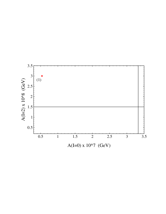
Figure 1: The starting point (1).

The starting point is computed in the absence of QCD corrections. In this case we have only one operator, $Q_{2}$, and:

$$A_{0}=\langle Q_{2}\rangle_{0}=\frac{2}{3}X\qquad A_{2}=\langle Q_{2}\rangle_{2}=\frac{\sqrt{2}}{3}X$$ (2.1)

where $X\equiv\sqrt{3}f_{\pi}\left(m_{K}^{2}-m_{\pi}^{2}\right)$. Fig. 1 illustrates how far the amplitudes thus obtained are from the experimental values.

3 NLO QCD Wilson Coefficients

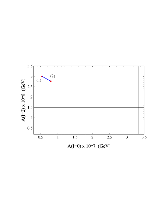
Figure 2: The effect of NLO QCD renormalization: point(2).

The first effect of having QCD in the game is the renormalization group evolution of the Wilson coefficients [6]. To give an idea of it, I collected in Table 1 the relevant next-to-leading-order (NLO) coefficients.

$\Lambda_{QCD}^{(4)}$	250 MeV		350 MeV
$\alpha_{s}(m_{Z})_{\overline{MS}}$	0.113		0.119
(HV) $\quad\mu=0.8$ GeV
$z_{1}$	$(0.0320)$	$-0.657$	$(0.0339)$	$-0.910$
$z_{2}$	$(0.988)$	$1.38$	$(0.987)$	$1.58$
$z_{3}$		$0.0137$		$0.0301$
$z_{4}$		$-0.0292$		$-0.0540$
$z_{5}$		$0.0070$		$0.0100$
$z_{6}$		$-0.0275$		$-0.0515$
$z_{7}/\alpha$		$-0.0055$		$-0.0030$
$z_{8}/\alpha$		$0.0198$		$0.0379$
$z_{9}/\alpha$		$0.0070$		$0.0203$
$z_{10}/\alpha$		$-0.0181$		$-0.0330$

Table 1: The NLO Wilson coefficients for the ten effective operators (as computed in the HV scheme). The initial values at $m_{W}$ are between brackets.

Fig. 2 makes clear that, while the effect goes in the right direction, it is by far too small to account for the rule.

4 Chiral Quark Model

In order to proceed we must estimate the hadronic matrix elements. Neither the lattice nor the $1/N_{c}$ approach can reproduce the rule. Notice that the leading $1/N_{c}$ corrections make $A_{2}$ bigger and do not help.

I will use the chiral quark model [7] ($\chi$QM) that is as simple a model as it is possible without having to renounce those features that we deem crucial in the understanding of the rule. It is defined by the following lagrangian

$${\cal{L}}_{\chi\mbox{\scriptsize QM}}=-M\left(\overline{q}_{R}\;\Sigma q_{L}+\overline{q}_{L}\;\Sigma^{\dagger}q_{R}\right)$$ (4.1)

that dictates the interaction between Goldstone bosons and quarks and therefore allows us to estimate the relevant hadronic matrix elements.

5 Penguin Operators

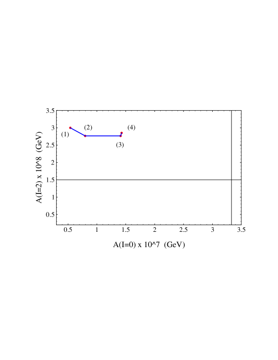
Figure 3: Penguin operators correction. Point (3) is the gluon Penguins; point (4) the electroweak ones. $\left\langle\bar{q}q\right\rangle=(-0.250\mbox{MeV})^{3}$.

A further important step in understanding the enhancement of the $A_{0}$ amplitude comes from the QCD-induced penguin operators [8] that only affect the $I=0$ amplitudes. In the $\chi$QM I find:

$$\langle Q_{3}\rangle_{0}=\frac{1}{N_{c}}X\quad\langle Q_{4}\rangle_{0}=X\quad\langle Q_{5}\rangle_{0}=\frac{2}{N_{c}}\,\frac{\langle\bar{q}q\rangle}{Mf_{\pi}^{2}}\,X^{\prime}\quad\langle Q_{6}\rangle_{0}=2\,\frac{\langle\bar{q}q\rangle}{f_{\pi}^{2}M}\,X^{\prime}\,,$$ (5.1)

where $X^{\prime}\equiv X\left(1-6\ M^{2}/\Lambda_{\chi}^{2}\right)$. Fig. 3 shows their effect.

6 Non-Factorizable Gluon Corrections

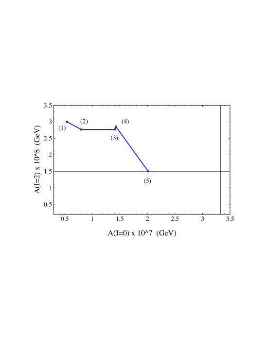
Figure 4: Nonperturbative gluon corrections: point (5).

Another, and, as we shall see essential, effect of QCD in the chiral quark model, arises from the soft-gluon corrections to the matrix elements [9]. These are parametrized by

$$\delta_{\langle GG\rangle}=\frac{N_{c}}{2}\frac{\langle\alpha_{s}GG/\pi\rangle}{16\pi^{2}f^{4}}$$ (6.1)

where I take for the non-perturbative gluon condensate

$$\langle\alpha_{s}GG/\pi\rangle=(350\mbox{MeV})^{4}\,,$$ (6.2)

a value that is consistent with current QCD sum rule estimates [10]. The effect of this correction is

$$\begin{array}[]{rclrcl}\langle Q_{1}\rangle_{0}&=&\frac{1}{3}X\left[-1+\frac{2}{N_{c}}\left(1-\delta_{\left\langle GG\right\rangle}\right)\right]&\qquad\langle Q_{1}\rangle_{2}&=&\frac{\sqrt{2}}{3}X\left[1+\frac{1}{N_{c}}\left(1-\delta_{\left\langle GG\right\rangle}\right)\right]\\ \langle Q_{2}\rangle_{0}&=&\frac{1}{3}X\left[2-\frac{1}{N_{c}}\left(1-\delta_{\left\langle GG\right\rangle}\right)\right]&\qquad\langle Q_{2}\rangle_{2}&=&\frac{\sqrt{2}}{3}X\left[1+\frac{1}{N_{c}}\left(1-\delta_{\left\langle GG\right\rangle}\right)\right]\\ \langle Q_{3}\rangle_{0}&=&\frac{1}{N_{c}}X\left(1-\delta_{\left\langle GG\right\rangle}\right)&\qquad\langle Q_{4}\rangle_{0}&=&X\\ \langle Q_{5}\rangle_{0}&=&\frac{2}{N_{c}}\,\frac{\langle\bar{q}q\rangle}{Mf_{\pi}^{2}}\,X^{\prime}&\qquad\langle Q_{6}\rangle_{0}&=&2\,\frac{\langle\bar{q}q\rangle}{f_{\pi}^{2}M}\,X^{\prime}\,.\end{array}$$ (6.3)

Fig. 4 shows how much this correction helps in going in the right direction. The amplitude $A_{2}$ is brought to its experimental value.

7 Chiral Loop Corrections

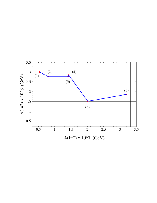
Figure 5: Effect of the chiral loops: point (6)

The amplitude $A_{0}$ is still too small. Meson loops [11] give the final enhancement. Fig. 5 shows how their effect is large for the $A_{0}$ amplitude and small for the $A_{2}$, as it should be in order to agree with the the selection rule.

8 The Final Point

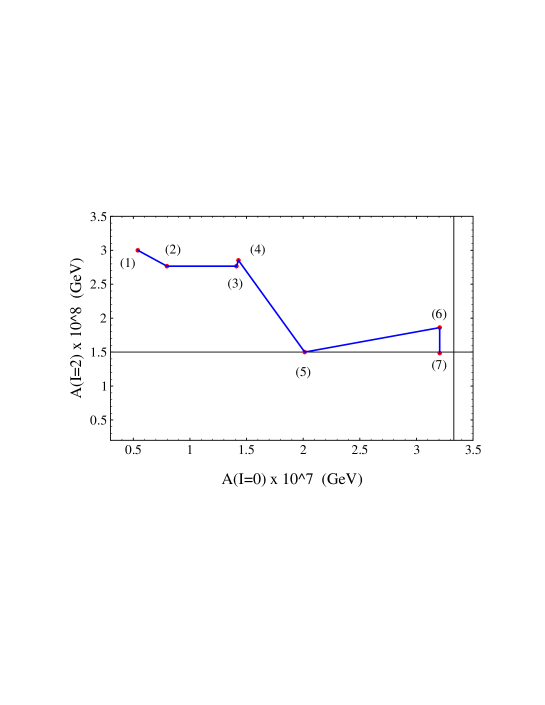
Figure 6: The final point (7).

Finally we must include the iso-spin breaking correction to $A_{2}$; it is proportional to $A_{0}$ and given by

$$A_{2}^{\rm iso-brk}\simeq-\frac{1}{3\sqrt{2}}\frac{m_{d}-m_{u}}{m_{s}}A_{0}$$ (8.1)

Fig. 6 includes such a correction and shows the final result. As it can be seen, the selection rule is now well reproduced.

9 Dependence on Input Parameters

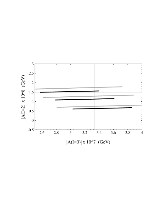
Figure 7: Input parameter dependence. Grey (black) lines are in the NDR (HV) scheme.

While the previous figures plotted a single point which corresponded to a fixed value for the input parameters, the dependence on them is rather strong as shown in Fig. 7 where I varied the quark condensate as

$$-(200\>\mbox{MeV})^{3}\leq\left\langle\bar{q}q\right\rangle\leq-(280\>\mbox{MeV})^{3}$$ (9.1)

and the gluon condensate as

$$(346\>\mbox{MeV})^{4}\leq\langle\frac{\alpha_{s}}{\pi}GG\rangle\leq(386\>\mbox{MeV})^{4}$$ (9.2)

for fixed $M=180\>\mbox{MeV}$ at $\mu=0.8\>\mbox{GeV}$.

Because of this intrinsic uncertainty, the best strategy consists in using the $\Delta I=1/2$ rule to restrict the input parameters and then use the matrix elements thus determined to predict new physical observable like, for instance, $\varepsilon^{\prime}/\varepsilon$ [12].

10 Scale and Matching Dependence

There is also a residual matching dependence that is described in Table 2. As shown by the two last lines of the table, the scale dependence is below the 20% level, as opposed to that before meson-loop renormalization which is as large as 40%.

$\Lambda^{(4)}_{\rm QCD}$ = 350 MeV
	$\mu=0.8$ GeV		$\mu=0.9$ GeV		$\mu=1$ GeV
	NDR	HV	NDR	HV	NDR	HV
$A_{0}$	2.97	2.94	2.66	2.61	2.45	2.39
$A_{2}$	1.60	1.46	1.68	1.56	1.75	1.64
$\Delta_{\gamma_{5}}A_{0}$	$1\%$		$2\%$		$2\%$
$\Delta_{\gamma_{5}}A_{2}$	$9\%$		$8\%$		$6\%$
$\Delta_{\mu}A_{0}$	$19\%-20\%$
$\Delta_{\mu}A_{2}$	$9\%-12\%$

Table 2: Matching dependence. $M\simeq 160\>\mbox{MeV}$, $\left\langle\bar{q}q\right\rangle$ at its PCAC value and $\left\langle\alpha_{s}/\pi GG\right\rangle=(376\>\mbox{MeV})^{4}$.

References

• [1] Review of Particle Properties, Phys. Rev. D 50 (1994) 1173.
• [2] M. Gell-Mann and A. Pais, Proc. Glasgow Conf. 1954, p. 342 (Pergamon, London, 1955).
• [3] H.-Y. Cheng, Int. J. Mod. Phys. A 4 (1989) 495.
• [4] V. Antonelli, S. Bertolini, M. Fabbrichesi and E.I. Lashin, Nucl. Phys. B 469 (1996) 181.
• [5] W.A. Bardeen A.J. Buras and J.-M. GΓ©rard, Phys. Lett. B 192 (1987) 138 and Nucl. Phys. B 293 (1987) 787.
• [6] K.G. Wilson, Phys. Rev. 179 (1969) 1499; M.K. Gaillard and B.W. Lee, Phys. Rev. Lett. 33 (1974) 108; G. Altarelli and L. Maiani, Phys. Lett. B 52 (1974) 351; A.J. Buras, M. Jamin and M.E. Lautenbacher, Nucl. Phys. B 408 (1993) 209; M. Ciuchini, E. Franco, G. Martinelli and L. Reina, Nucl. Phys. B 415 (1994) 403; Phys. Lett. B 301 (1993) 263.
• [7] K. Nishijima, Nuovo Cim. 11 (1959) 698; F. Gursey, Nuovo Cim. 16 (1960) 230 and Ann. Phys. (NY) 12 (1961) 91; J.A. Cronin, Phys. Rev. 161 (1967) 1483; S. Weinberg, Physica 96A (1979) 327; A. Manohar and H. Georgi, Nucl. Phys. B 234 (1984) 189; A. Manohar and G. Moore, Nucl. Phys. B 243 (1984) 55.
• [8] M.A. Shifman, A.I. Vainshtein and V.I. Zakharov, Nucl. Phys. B 120 (1977) 316; Y. Dupont and T.N. Pham, Phys. Rev. D 29 (1984) 1368; J.F. Donoghue, Phys. Rev. D 30 (1984) 1499; M.B. Gavela et al., Phys. Lett. B 148 (1984) 225; R.S. Chivukula, J.M. Flynn and H. Giorgi, Phys. Lett. B 171 (1986) 453.
• [9] D. Espriu, E. de Rafael and J. Taron, Nucl. Phys. B 345 (1990) 22; A. Pich and E. de Rafael, Nucl. Phys. B 358 (1991) 311.
• [10] E. Braaten, S. Narison and A. Pich, Nucl. Phys. B 373 (1992) 581; S. Narison, Phys. Lett. B 361 (1995) 121; R.A. Bertlmann et al., Z. Physik C 39 (1988) 231; C.A. Dominguez and E. de Rafael, Ann. Phys. (NY) 174 (1987) 372.
• [11] G. Kambor, J. Missimer and D. Wyler, Nucl. Phys. B 346 (1990) 17 and Phys. Lett. B 261 (1991) 496; V. Antonelli, S. Bertolini, J. Eeg, M. Fabbrichesi and E.I. Lashin, Nucl. Phys. B 469 (1996) 143.
• [12] S Bertolini, J.O. Eeg and M. Fabbrichesi, A New Esitimate of $\varepsilon^{\prime}/\varepsilon$, preprint SISSA 103/95/EP to appear in Nuclear Physics B.
• [13]