31 May 96 final version

the1.tex 31 May 96 alf

1 Introduction

The so-called principle of multiple point criticality[1, 2, 3, 4] states that Nature - in for example a field theory - seeks out values of action parameters that are located at the junction of a maximum number of phases in a phase diagram of a system that undergoes phase transitions. The phases to which we here ascribe physical importance are normally regarded as artifacts of a calculational regulation procedure. This latter often takes the form of a lattice. Contrary to the notion that a regulator is just a calculational device, we claim that the consistency of any field theory in the ultraviolet limit requires an ontological fundamental scale regulator. In light of this claim, the “lattice artifact” phases of, for example, a lattice gauge theory acquire the status of physically distinguishable fluctuation patterns at the scale of the fundamental regulator that can have important consequences for fundamental physics.

We have applied the principle of multiple point criticality[1, 3, 4] to the system of different (Planck scale) lattice phases that can be provoked using a suitably generalised action in a lattice gauge theory with a gauge group that is taken to be a Planck scale predecessor to the Standard Model Group (SMG) - namely the $N_{gen}$-fold Cartesian product of the SMG (here $N_{gen}$ denotes the number of fermion generations). This gauge group, denoted as $SMG^{N_{gen}}$, is referred to as the Anti Grand Unified Theory (AGUT) gauge group. The number of generations $N_{gen}$ is taken to be three in accord with experimental evidence; the AGUT gauge group $SMG^{3}$ has one $SMG$ factor for each family of quarks and leptons. Ambiguities that arise under mappings of the gauge group $SGM^{3}$ onto itself result in the Planck scale breakdown to the diagonal subgroup of $SMG^{3}$. The diagonal subgroup is isomorphic to the usual standard model group.

In the context of a Yang-Mills lattice gauge theory, the principle of multiple point criticality states that Nature seeks out the point in the phase diagram at which a maximum number of phases convene. This is the multiple point. The physical values of the three SMG gauge couplings at the Planck scale are predicted to be equal to the diagonal subgroup couplings corresponding to the multiple point action parameters of the Yang Mills lattice gauge theory having as the gauge group the AGUT gauge group $SMG^{3}$. It is indeed truly remarkable that this prediction leads to agreement with experiment to within 10 % for the non-Abelian couplings and 5% for the U(1) gauge coupling. For the Abelian as well as the non-Abelian cases, the deviation is of the order of the calculational uncertainty.

In order to compare Planck scale predictions for gauge coupling constants with experiment, it is of course necessary to extrapolate experimental values to the Planck scale. This is done with a renormalization group extrapolation in which a “desert” scenario is assumed. It should be emphasised that the prediction put forth here for the gauge couplings using our model with the AGUT gauge group $SMG^{3}$ is incompatible with the currently popular $SU(5)$ or $SU(5)$ super-symmetric grand unified models and is therefore to be regarded as a rival to these.

In a more general context, the Multiple Point Criticality Principle (MPCP) is proposed as a fundamental principle of Nature that also may be able to explain essentially all of the well known fine-tuning enigma in high energy physics[5, 6, 2]. Indeed, the conspicuous values assumed by many physical constants (e.g., fine-structure constants, the vanishing effective cosmological constant, the smallness of Higgs mass compared to Planck scale, $\Theta_{QCD}$) seem to coincide with values that are obtained if one assumes that Nature in general seeks out multiple point values for intensive parameters.

Multiple point values of intensive parameters could be explained - indeed, would be expected - by having the presence of many coexisting phases separated by first order transitions. Phase coexistence would be enforced for many combinations of universally fixed but not fine-tuned amounts of extensive quantities. The intensive parameters conjugate to such extensive quantities would then have fine-tuned values. And the higher the degree of first-orderness of the phase transition between the coexisting phases, the greater the number of combinations of the extensive quantities that could only be realized by having coexisting phases. As a useful illustrative prototype, one can think of an equilibrium system consisting of a container within which there is water in all three phases: solid, liquid, and ice. If the container is rigid and also impenetrable for heat and water molecules, we have accordingly the fixed amounts of the extensive quantities energy, mole number of water, and volume. If these quantities are fixed at values within some rather wide ranges, the fact that the heats of melting, vaporisation, and sublimation are finite forces the system to maintain the presence of all three phases of water. The permanent coexistence of all three phases accordingly “fine-tunes” the values of the intensive parameters temperature and pressure to those of the triple point of water.

However, having fixed amounts of such extensive quantities is tantamount to having long range non-local interactions of a special type: these interactions are identical between fields at all pairs of space-time points regardless of the space-time distance between them. Such omnipresent nonlocal interactions, which are present in a very general form of a reparameterization invariant action[7], would not be perceived as “action at a distance” but rather most likely incorporated into our theory as constants of Nature. Hence one can speculate[5, 6] that this mild form of non-locality is the underlying explanation of Nature’s affinity for the multiple point. We also speculate that nonlocal effects, described by fields depending on two space-time points, may be responsible for the replication of the fields in three generations[6]. Such a nonlocal mechanism would also triple the number of boson fields. As this feature is inherent to the AGUT model, a tripling of boson fields is a welcome prediction.

Originally, the MPCP was suggested on phenomenological grounds in conjunction with the development of methods for constructing phase diagrams for lattice gauge theories with non-simple gauge groups. These methods have been used to implement the MPCP in the most recent of a series of models that have been developed with the aim of calculating the standard model gauge coupling constants.

Indeed, the theoretical calculation of the fine structure constant $\alpha=1/137.0360...$ and the other Yang Mills coupling constants, the information content of which is identical to that of the Weinberg angle $\theta_{W}$ and the scale parameter $\Lambda_{\overline{MS}}$, continues to pose a challenge to be surmounted by theories at a more fundamental level.

The Multiple Point Criticality Principle (MPCP), developed by Holger Bech Nielsen and me, is but one of the more recent results in a long series of interwoven projects involving many people in which the undisputed central figure and prime instigator has been my teacher and colleague Holger Bech Nielsen. In the course of the last 15 years or so, I have also had the privilege of working together with H.B. Nielsen and others on several other projects some of which have been predecessors to the multiple point criticality idea. Also included among the projects to which I have contributed is some of the work on Random Dynamics. The philosophy of Random Dynamics is the creation of H. B. Nielsen[8] and came to my attention over 15 years ago[9, 10, 11].

Section 2 reviews some earlier work belonging more or less directly to the convoluted ancestry of the multiple point criticality idea. Being somewhat historical, the presentation in this Section is not logically streamlined but rather emphasises the inspirational role that Random Dynamics has played in a number of contexts that somehow are part of the lineage of the multiple point criticality principle. Section 2.1 describes a sort of forerunner to the MPCP that has emerged in a number of models considered - namely an inequality relating gauge couplings at the Planck scale, the number $N_{gen}$ of quark and lepton generations and the critical couplings in a lattice gauge theory. Section 2.2 describes the AGUT gauge group $SMG^{N_{gen}}$ which is inextricably interwoven with the development of the multiple point criticality principle and various Random Dynamics-inspired models. The AGUT gauge group

$$SMG^{N_{gen}}\stackrel{{\scriptstyle def}}{{=}}\underbrace{SMG\times SMG\times\cdots\times SMG}_{N_{gen.}\mbox{ \footnotesize Cartesian product factors}}.$$ (1)

is assumed to be a more fundamental predecessor to the phenomenologically established standard model group. The latter arises as the diagonal subgroup of $SMG^{N_{gen}}$ that survives the Planck scale breakdown of $SMG^{N_{gen}}$. In particular, this Section describes the way that inverse squared gauge couplings are enhanced by a $N_{gen}$-related factor in conjunction with the breakdown to this diagonal subgroup. By definition, the diagonal subgroup of $SMG$ has excitations of the (group valued) lattice link variables that are identical for each of the $N_{gen}$ Standard Model Group factors of $SMG^{3}$. The philosophy of Random Dynamics is sketched in Section 2.3. The Random Dynamics approach is used in the rather lengthly Section 2.4 to “derive” gauge symmetry in the context of a field theory glass. This Section develops and relates many ideas the rudiments of which have been presented by H.B. Nielsen in lectures given at his inspiring course series “Q.C.D. etc”. This legendary course is a veritable forum of new ideas in physics. The so-called “confusion” mechanism by which the AGUT gauge group $SMG^{3}$ breaks down at the Planck scale to its diagonal subgroup is reviewed in Section 2.5. This happens as a result of ambiguities that arise under group automorphic symmetry operations. The AGUT gauge group is viewed as the final link in a chain of increasingly robust SMG predecessors selected by Random Dynamics in going to lower and lower energies at roughly the Planck scale. In Section 2.6, a model with a string-like regularization in a Kaluza-Klein space-time at the fundamental scale is used to derive the inequality of Section 2.1.

Section 3 is devoted to the Multiple Point Criticality Principle (MPCP). Though the MPCP was from the start formulated in the context of a lattice gauge theory in order to predict standard model gauge coupling constants, generalisations[4, 12, 5, 6, 2] in the formulation and applicability of this principle have been considered. Multiple point criticality as a way of explaining “fine-tuned” quantities in Nature is discussed in Section 3.1. This fine-tuning mechanism entails having universally fixed amounts of extensive quantities conjugate to intensive quantities (e.g., fine-structure constants); these latter have a finite probability for being fine-tuned that increases as the number of combinations of extensive variables that cannot be realized as a single phase becomes larger. However, having universally fixed amounts of extensive quantities actually implies having a mild form of non-locality that is analogous to that inherent to a micro-canonical ensemble in statistical mechanics: an inherent feature of a micro-canonical ensemble is the introduction of long range correlations that strictly speaking breaks locality. However it has been shown [7] that non-locality of the type analogous to that introduced by the assumption of a micro-canonical ensemble is harmless insofar as it does not lead to experimentally observable violations of locality. Multiple point criticality as related to the problem of fine-tuning and the presence of non-locality is discussed at some length in Section 3.2.

Section 4 deals with the phases distinguishable at the scale of the lattice in a lattice gauge theory implementation of the MPCP. The junction in the phase diagram to which the maximum number of such phases are adjoined is sought out for the purpose of determining gauge coupling constants. Such phases are really what would normally be regarded as “lattice artifacts”. However, in light of our philosophy that a lattice is one of perhaps many ways of implementing what is assumed to be the necessity of a ontological Planck scale regulator, these “artifact phases” acquire a physical meaning. These phases are governed by which micro physical fluctuation patterns yield the maximum value of $\log Z$ where $Z$ is the partition function. Qualitatively different short distance physics could consist of different distributions of group elements along various subgroups for different regions of (bare) plaquette action parameter space. For example, if in going from one region of parameter space to another, the correlation length goes from being shorter than the lattice constant to being of the order of several lattice constants, we would see a transition from a confining to a “Coulomb phase” if the determination of phase was done at the scale of the lattice. Even if such different lattice scale phases become indistinguishable in going to long wavelengths because such phases turn out to be confining, this in no way precludes physical significance for lattice-scale phases that come about as a result of a physically existing fundamental regulator. At the scale of what is assumed to be the fundamental regulator, there is a distinguishable “phase” for each invariant subgroup $H$ of a non-simple gauge group $G$ including discrete (invariant) subgroups. Any invariant subgroup $H$ of the gauge group $G$ labels a confinement-like phase the defining feature of which is that Bianchi variables (i.e., the variables that must coincide with the unit element in order that the Bianchi identity be fulfilled) have a distribution on the group such that essentially all elements of $H$ would be accessed by quantum fluctuations if the fluctuations in the plaquette variables did not have to be correlated in such a way as the fulfil the Bianchi identities. So a phase confined w.r.t. $H$ has appreciable quantum fluctuations along $H$ while the degrees of freedom corresponding to the cosets of the factor group $G/H$ have a distribution peaked at the coset for which the identity of $G$ is a representative. These latter degrees of freedom are said to have Coulomb-like behaviour. Such a phase is often referred to as a partially confining phase . The classification of these partially confining phases is the subject of Section 4.4.

Section 5 addresses the problem of distinguishing all (or some chosen set) of the possible partially confining phases (with each phase corresponding to an invariant subgroup $H$). This requires using a class of plaquette actions general enough to provoke these phases. Some general features of such actions are examined in Section 5.1. Phase diagrams for non-simple gauge groups suitable for seeking the multiple point are considered in Sections 5.2 and 5.3. Section 5.4 outlines problems encountered in implementing the principle of multiple point criticality in the case of $U(1)$ (or $U(1)^{3}$) as compared to the simpler case of the non-Abelian subgroups of the standard model. One of these problems, related to the “Abelian-ness” of $U(1)$, is a result of the interactions between the $N_{gen}$ replicas of $U(1)$ in the AGUT gauge group $SMG^{3}$. In the roughest approximation, these interactions result in a weakening of the diagonal subgroup coupling of $U(1)\in SMG^{3}$ by a factor of $\frac{1}{2}N_{gen}(N_{gen}+1)=6$ instead of the weakening factor $N_{gen}=3$ that applies to the non-Abelian subgroups (for which such interaction are not gauge invariant).

In constructing actions suitable for implementing the MPCP for the purpose of determining gauge couplings, we reach in Section 6 a point in the development where it is expedient to consider separately the Abelian and non-Abelian couplings. The simpler case of the non-Abelian couplings is treated first in Section 6 followed by the Abelian case in Sections 7 and 8. These latter two sections contain the essence of very recent work[1].

Section 6 deals with the determination of the multiple point couplings (with the AGUT gauge group $SMG^{3}$) for the non-Abelian subgroups of the $SMG$. After writing down some formalism in Section 6.1, the a priori lack of universality of the model is discussed in Section 6.1.1 inasmuch as the phase transitions at the multiple point are typically at first order. However, our restriction on the form of the plaquette action nurtures the hope of at least an approximate universality. Section 6.2 develops a modified Manton action that leads to distributions $e^{S_{\Box}}$ of group-valued plaquette variables consisting of narrow maxima centred at elements $p$ belonging to certain discrete subgroups of the centre of the gauge group. The action at these peaks is then expressed as truncated Taylor expansions around the elements $p$. With this action ansatz, it is possible to provoke confinement-like or Coulomb-like behaviour independently (approximately at least) for the 5 “constituent” invariant subgroups $\mbox{\bf{Z}}_{2},\;\mbox{\bf{Z}}_{3},\;U(1),\;SU(2),$ and $SU(3)$ of the SMG which “span” the set of “all” invariant subgroups of the SMG. In our approximation, the mutually un-coupled variation in the distributions along these 5 “constituent” invariant subgroups is accomplished using 5 action parameters: 3 parameters $\beta_{1},\;\beta_{2},$ and $\beta_{3}$ that allow adjustment of peak widths in the $U(1),\;SU(2),$ and $SU(3)$ directions on the group manifold and 2 parameters $\xi_{2}$ and $\xi_{3}$ that make possible the adjustment of the relative heights of the peaks centred at elements $p\in\mbox{span}\{\mbox{\bf{Z}}_{2},\mbox{\bf{Z}}_{3}\}$. A lengthly digression in Section 6.4 develops techniques for constructing phase diagrams for non-simple gauge group in the simpler approximation in which phases solely confined w.r.t discrete subgroups are not included. Methods for constructing phase diagrams also having this latter type of phase (which are necessary for having a multiple point) are then considered in Section 6.5. Correction due to quantum fluctuations are considered in Section 6.6. The first four Appendices 11.1, 11.2, 11.3 and 11.4, which are not essential to the continuity of the thesis, deal with various improvements to the methods of constructing approximate phase diagrams considered in Section 6. In Appendix 11.4 for example, interactions between the “constituent” invariant subgroups mentioned above are considered.

Section 7 considers the gauge group $U(1)^{3}$ that is used as an approximation to the AGUT $SMG^{3}$ for the purpose of determining the $U(1)$ gauge coupling. The normalisation problems with $U(1)$ are considered in Sections 7.1.1, 7.1.2 and 7.1.3. Phase diagrams for the gauge group $U(1)^{3}$ in which we can seek out multiple point parameter values are needed. In Section 7.2, a formalism is developed that allows us to seek multiple point parameter values by adjusting the metric (which amounts to adjusting the parameters of a Manton action) in a $N_{gen}$-dimensional space upon which is superimposed an hexagonally symmetric lattice of points identified with the identity of $U(1)^{3}$. The hexagonal symmetry takes into account the allowed interactions between the $N_{gen}=3$ $U(1)$ factors of $U(1)^{3}$. Using this formalism, two approximative methods of determining phase boundaries are developed: the independent monopole approximation (Section 7.3.1) and the group volume approximation (Section 7.3.2). These describe respectively phase transitions that are purely second order and strongly first order.

Section 8 is devoted to calculations where we interpolate between the extreme situations described by the group volume and independent monopole approximations. This interpolation is done by calculating the discontinuity $\Delta\gamma_{eff}$ at the multiple point in an effective coupling $\gamma_{eff}$ (introduced in Section 8.2). In Section 8.3 it is seen that the dominant contributions to $\Delta\gamma_{eff}$ are due to multiple point transitions between phases that differ by the confinement of discrete subgroups (rather than continuous subgroups). The calculated $\Delta\gamma_{eff}$ reflects the degree of first-orderness of these transitions. As a result of including this effect, the weakening factor $N_{gen}(N_{gen}+1)/2=6$ is seen in Section 8.4 to increase to about 6.5. The quantity $\Delta\gamma_{eff}$ is also used (together with $\gamma_{eff}$) to calculate the continuum $U(1)$ coupling corresponding to the multiple point of a single $U(1)$ in Section 8.5. In the tables at the end of Section 8.5, this value of the continuum $U(1)$ coupling is multiplied by the weakening factor of about 6.5 (calculated in Section 8.4) to get our prediction for the value of the running $U(1)$ coupling at the Planck scale.

Section 9 presents the results from multiple point criticality for all three gauge couplings. Values are given at the Planck scale as well as at the scale of $M_{Z}$. The latter are obtained using the assumption of the minimal standard model in doing the renormalization group extrapolation. In the case of $U(1)$, a number of slightly different values are presented that reflect the differences that arise due to approximations that differ in how some details are treated. In presenting what we take to be the “most correct” result, we compute the uncertainty from the deviations arising from plausibly correct ways of making distinctions in how different discrete subgroups enter into the calculation of $\Delta\gamma_{eff}$. The value of $\alpha^{-1}$ predicted from multiple point criticality is calculated to be $136.8\pm 9$. This is to be compared with the experimental value of $137.036\cdots$. The thesis ends with some concluding remarks.

Although the presentation of the current state of the MPC model for predicting gauge coupling constants and the techniques devised for implementing it will constitute the major part of this thesis, earlier work will be reviewed and the most recent developments in ongoing work will be included.

2 History of the project including the inspirational role of Random Dynamics

2.1 A Planck scale inequality relating gauge coupling to number of fermion generations

The evolution of the MPC model for predicting the Standard Model gauge coupling constants is inseparably tied together with the ideas of Random Dynamics as well as speculations as to the origins of the SMG and the number $N_{gen}$ of generations of fermions. The work preceding the MPC principle has involved a number of models all of which lead to or at least suggest features of an inequality relating the gauge coupling constants at the Planck scale, the number $N_{gen}$ of quark and lepton generations, and the critical values of inverse squared gauge couplings $\beta_{crit}$ in a regularised (i.e., latticised in most cases) gauge theory:

$$\beta_{experimental}(\mu_{Planck})\geq N_{gen}\beta_{crit}$$ (2)

This inequality, originally suggested on phenomenological grounds[13, 14, 15, 16, 17, 18], is, when supplemented with arguments for why it is realised in Nature as an equality, the forerunner of the multiple point criticality idea. Various “derivations” of this inequality share some common and interrelated features (that, depending on which model is considered, are used as assumptions or show up as consequences):

1. The phenomenologically observed Standard Model Group (SMG) is, at the fundamental ($\approx$ Planck) scale, replicated a number of times. The Cartesian product of these replicas of the SMG, assumed to be a predecessor to the usual SMG, breaks down at the Planck scale to the diagonal subgroup of the Cartesian product.

2. In order to be phenomenologically relevant, the replicas of the Standard Model Group at the fundamental scale must have coupling constants that are on the weak coupling side of the “critical” value in order to avoid a confinement-like phase already at the fundamental scale. This amounts to an upper bound on allowed Planck scale couplings.

3. The Planck scale criticality referred to in 2. pertains to transitions between “phases” that conventionally would be regarded as artifacts of the regularization procedure used (which, for almost all the models considered up to now, means a lattice). Ascribing physical significance to such “phases” is tantamount to assuming the existence of a regulator as an intrinsic property of fundamental scale physics.

4. The upper bound on Planck couplings for the SMG replicas appears to be saturated; i.e., couplings assume the largest possible (i.e., critical) values that are consistent with avoiding confinement. This feature, which may be necessary in order to avoid a Higgsed phase at the Planck scale, is intrinsic to the idea of MPC.

5. It is assumed that the more fundamental Cartesian product gauge group assumed in 1. above contains (at least) one SMG factor for each generation of quarks and leptons. Collaboration of the $N_{gen}$ replicated SMG factors near the Planck scale reduces the gauge symmetry from that of the Cartesian product group to that of the diagonal subgroup (which of course is isomorphic to the usual SMG). Assuming the validity of the saturation property in 4. above for each SMG factor in the Cartesian product gauge group, this spontaneous reduction in the gauge symmetry is accompanied by an enhancement in the values of the three SMG inverse squared gauge couplings of the diagonal subgroup by a factor equal to the number $N_{gen}$ of quark and lepton generations. This was originally suggested on phenomenological grounds: early on the observation was made that the magnitude of the non-Abelian gauge coupling constants is of the order one divided by the square root of the number of generations $N_{gen}$ provided that unit coupling strength is taken to be that at the transition between the confined and Coulomb phases in the mean field approximation.

2.2 The Anti Grand Unified Theory Gauge Group (AGUT Gauge Group) SMG³

As mentioned several times already, a central feature that emerges or that at least is suggested in the context of various different models is that the phenomenologically well-established Standard Model Group SMG stems from a more fundamental predecessor referred to as the “anti-grandunified theory” (AGUT) gauge group and denoted by $SMG^{N_{gen}}$. This group is the $N_{gen}$-fold Cartesian product of essentially SMG factors with one SMG factor for each of the $N_{gen}$ generations of quarks and leptons. In terms of the Lie algebra

$$SMG^{N_{gen}}\stackrel{{\scriptstyle def}}{{=}}$$ (3)

$$=\underbrace{U(1)\times U(1)\times\cdots\times U(1)}_{N_{gen}}\times\underbrace{SU(2)\times SU(2)\times\cdots\times SU(2)}_{N_{gen}}\times\underbrace{SU(3)\times SU(3)\times\cdots\times SU(3)}_{N_{gen}}.$$

The identification of the number of SMG factors in the Cartesian product $SMG^{N_{gen}}$ with the number of families $N_{gen}$ allows the possibility of having different gauge quantum numbers for the $N_{gen}$ different families. The integer $N_{gen}$ designates the number of generations and is taken to have the value $N_{gen}=3$ in accord with experimental results.

In this work, an alternative to the usual Standard Model Group $U(1)\times SU(2)\times SU(3)$ will be used; here the Standard Model Group (SMG) is defined as

$$SMG\stackrel{{\scriptstyle def.}}{{=}}S(U(2)\times U(3))\stackrel{{\scriptstyle def.}}{{=}}\left\{\left.\left(\begin{array}[]{cc}\mbox{\bf{U}}_{2}&\begin{array}[]{ccc}0&0&0\\ 0&0&0\end{array}\\ \begin{array}[]{cc}0&0\\ 0&0\\ 0&0\end{array}&\mbox{\bf{U}}_{3}\end{array}\right)\right|\begin{array}[]{l}\mbox{\bf{U}}_{2}\in U(2),\\ \mbox{\bf{U}}_{3}\in U(3),\\ \mbox{det}\mbox{\bf{U}}_{2}\cdot\mbox{det}\mbox{\bf{U}}_{3}=1\end{array}\right\}$$ (4)

This group is suggested by the representation spectrum of the standard model[19]; it has of course the same Lie algebra as the more commonly used group $U(1)\times SU(2)\times SU(3)$.

The usual standard model description of high energy physics comes about as the diagonal subgroup of $SMG^{3}$:

$$SMG^{3}\stackrel{{\scriptstyle breakdown}}{{\longrightarrow}}(SMG^{3})_{diag.\;subgr.}\stackrel{{\scriptstyle def.}}{{=}}\{(g,g,g)\mid g\in SMG\}$$ (5)

resulting from the Planck scale breakdown of the gauge group $SMG^{3}$. The diagonal subgroup of $SMG^{3}$ is of course isomorphic to the SMG. The breakdown to the diagonal subgroup can come about due to ambiguities that arise under group automorphic symmetry operations. This is usually referred to as the “confusion” mechanism[20, 21, 22].

The breakdown of the group $SMG^{3}$ to the diagonal subgroup has consequences[23] for the SMG gauge couplings that we now briefly describe. Recalling that the diagonal subgroup of $SMG^{3}$ corresponds by definition to identical excitations of the $N_{gen}=3$ isomorphic gauge fields (with the gauge couplings absorbed) and using the names $Peter$, $Paul,\cdots$ as indices that label the $N_{gen.}$ different isomorphic Cartesian product factors of $(SMG)^{N_{gen.}}$, one has

$$(g{\cal A}_{\mu}(x))_{Peter}=(g{\cal A}_{\mu}(x))_{Paul}=\cdots=(g{\cal A}_{\mu}(x))_{N_{gen.}}\stackrel{{\scriptstyle def.}}{{=}}(g{\cal A}_{\mu}(x))_{diag.};$$ (6)

this has the consequence that the common $(gF_{\mu\nu})^{2}_{diag}$ in each term of the Lagrangian density for $(SMG)^{N_{gen.}}$ can be factored out:

$${\cal L}=-1/(4g_{Peter}^{2})(gF_{\mu\nu}^{a}(x))^{2}_{Peter}-1/(4g_{Paul}^{2})(gF_{\mu\nu}^{a}(x))^{2}_{Paul}-\cdots-1/(4g_{N_{gen.}}^{2})(gF_{\mu\nu}^{a}(x))^{2}_{N_{gen.}}$$ (7)

$$=(-1/(4g_{Peter}^{2})-1/(4g_{Paul}^{2})-\cdots-1/(4g_{N_{gen.}}^{2}))\cdot(F_{\mu\nu}^{a}(x))^{2}_{diag}=-1/(4g_{diag}^{2})\cdot(gF_{\mu\nu}^{a}(x))^{2}_{diag}.$$ (8)

The inverse squared couplings for the diagonal subgroup is the sum of the inverse squared couplings for each of the $N_{gen.}$ isomorphic Cartesian product factors of $(SMG)^{3}$. Additivity in the inverse squared couplings in going to the diagonal subgroup applies separately for each of the invariant Lie subgroups $i\in\{SU(2),SU(3)\}\subset SMG$. However, for $U(1)$ it is possible to have terms in the Lagrangian of the type $F_{\mu\nu}^{Peter}F^{\mu\nu\;Paul}$ in a gauge invariant way. Therefore it becomes more complicated as to how one should generalise this notion of additivity. Terms of this type can directly influence the $U(1)^{3}$ continuum couplings. But for the non-Abelian couplings we simply get

$$\frac{1}{g_{i,diag}^{2}}=\frac{1}{g_{i,Peter}^{2}}+\frac{1}{g_{i,Paul}^{2}}+\cdots+\frac{1}{g_{i,N_{gen}}^{2}}\;\;(i\in\{SU(2),\;SU(3)\}).$$ (9)

Assuming that the inverse squared couplings for a given $i$ but different labels $\{Peter,Paul,\cdots,N_{gen.}\}$ are all driven to the multiple point in accord with the principle of multiple point criticality (discussed at length in a later section), these $\{Peter,Paul,\cdots,N_{gen}\}$ couplings all become equal to the multiple point value $g_{i,multi.\;point}$; i.e.,:

$$\frac{1}{g_{i,Peter}^{2}}=\frac{1}{g_{i,Paul}^{2}}=\cdots=\frac{1}{g_{i,N_{gen}}^{2}}=\frac{1}{g_{i,\;multi.\;point}^{2}}.$$ (10)

It is seen that the inverse squared coupling $1/g_{i,\;diag}^{2}$ for the $i$th subgroup of the diagonal subgroup is enhanced by a factor $N_{gen}$ relative to the corresponding subgroup $i$ of each of the $N_{gen}$ Cartesian product factors $Peter$, $Paul,\cdots,N_{gen.}$ of $(SMG)^{N_{gen.}}$:

$$\frac{1}{g_{i,diag}^{2}}=\frac{N_{gen}}{g_{i,\;multi.\;point}^{2}}.$$ (11)

It is this weakening of the coupling for each of the subgroups $i\in\{SU(2),SU(3)\}$ of the diagonal subgroup (i.e., the SMG) that constitutes the main role of the anti-unification scheme in our model. Anticipating the later discussion of the role of the multiple point, we point out prematurely that while it is the $g_{i,\;multi.\;point}$ (i.e., $i=SU(2)$ or $SU(3)$) which are to be identified with the critical values (at the multiple point) of coupling constants for the bulk phase transition of a lattice Yang-Mills theory with gauge group $i$, it is the $g_{i,\;diag.}=g_{i,\;multi.\;point}/\sqrt{N_{gen.}}$ that, in the continuum limit, are to be identified with the corresponding experimentally observed couplings extrapolated to the Planck scale[24, 25].

The validity of the principle of multiple point criticality together with the assumption of the AGUT gauge group $SMG^{N_{gen}}$ as the immediate predecessor to the usual SMG at the Planck scale can be claimed to be justifiable a posteori alone on the grounds of phenomenological success in predicting gauge coupling constants. Even though the idea of multiple point criticality can stand alone as a model that predicts gauge coupling constants and as a plausible candidate for explaining fine-tuned quantities in Nature, I think it is important to emphasise the important inspirational role that Random Dynamics has played in developing the various models that culminated in the principle of multiple point criticality.

2.3 The philosophy of Random Dynamics

The idea behind Random Dynamics is outlined in this section. In the following three Sections 2.4, 2.5 and 2.6 three representative applications of Random Dynamics have been chosen from various models that motivate various aspects that have been important in arriving at what today refer to as the principle of multiple point criticality with AGUT gauge group. In Section 2.4 we present a field theory glass model for Planck scale physics that, in keeping with the idea of Random Dynamics, is proposed as being sufficiently general and unrestricted so as to have a good chance of yielding low energy physics (LEP) in the long wavelength limit. This Section ends with arguments that indicate that the phenomenologically suggested realisation of the inequality (2) as an equality can be understood in the context of a field theory glass. In Section 2.5, a brief review is given of a possible mechanism - the confusion mechanism - for the Planck scale breakdown of the AGUT gauge group $SMG^{3}$ to its diagonal subgroup. In Section 2.6 we discuss a model in which experimental couplings extrapolated to the Planck scale suggest constraints on the volume of the compactification space in a model with a Kaluza-Klein space-time. This leads to a constraint on the value of $N_{gen}$ as well as the scale at which grand-unification, if realised in Nature, could take place. All three models involve arguments suggested by the ideas of Random Dynamics.

The idea behind the Random Dynamics principle is that at very high energies (i.e., $\geq$ Planck energies), almost any model for fundamental physics that possesses sufficient complexity and generality will in the low energy limit (i.e., at energies accessible to experiment) yield physics as we know it. In other words, it is the constraints dictated by the process of taking the low energy limit (of a fundamental model for supra-Planck scale physics) that are decisive in determining the form of low energy physics. Taking this viewpoint means that essentially any (e.g., randomly chosen) model for supra-Planck scale physics will be shaped into low energy physics as we know it because the process of going to low energies “filters away” all features of any supra-Planck scale model except the features that characterise low energy physics. These latter features “survive” a sort of selection process that is assumed to be inherent in taking the long wavelength limit of any fundamental theory. The assertion that we get the same low energy physics (LEP) for almost any sufficiently general set of assumptions for fundamental scale physics suffices as a starting point for taking a long wavelength limit is equivalent to deriving LEP from almost no assumptions about fundamental scale physics. This is because few if any assumptions are so important that they couldn’t be excluded from some set of sufficiently general assumptions that would also yield LEP in the long wavelength limit.

2.4 Gauge symmetry from a field theory glass

Here a field theory glass[26, 27] is taken as the starting point for a Random Dynamics “derivation” of the gauge symmetry of the Standard Model description of LEP physics. By examining a field theory glass, one hopes to find as a generic possibility the approximate gauge symmetry needed as the starting point for the the FNNS gauge symmetry exactification mechanism[28]. Subsequently, we shall use the formal technique used in demonstrating the FNNS mechanism to argue that in a statistical sense MPC offers the best chance for reconciling a conflict between on one hand avoiding confinement and the other hand avoiding Higgsing.

The field theory glass is envisioned as residing in a discretized space-time. In other words, each physically realisable space-time event corresponds to a site in a very irregular lattice. As regards Lorentz invariance, which is obviously absent in this discretized space-time, the hope is that it can be recovered in the long wavelength limit.

Denoting the fundamental set of such space-time points as $\{j\}$, we define a generalised field $\phi$ that for each site $j$ takes values on a site-associated manifold ${\cal M}_{j}$. The site-associated manifolds ${\cal M}_{j}$, each of which is presumed to be individually very complicated, depend on $j$ in a quenched random way. The generalised field $\phi$ is described by the mapping [29, 26]

$$\phi:\{j\}\rightarrow\cup_{j}\{{\cal M}_{j}\}\;\mbox{ with the restriction}\;\phi(j)\in{\cal M}_{j}.$$ (13)

Having the field theory glass degrees of freedom, we want now to define a very general action subject to the constraint that (semi)locality is to be retained. This is accomplished by defining the action to be additive in contributions from small quenched randomly chosen space-time regions (generally overlapping) distinguished here by the index “$r$”: $S[\phi]=\sum_{r}S_{r}(\phi\mid_{r})$ where $\phi\mid_{r}$ denotes the restriction of the mapping $\phi$ to the sites $i\in r$. Each regional contribution $S_{r}$ to the action is a mapping $S_{r}$: $\times^{cart\;prod}_{j\in r}{\cal M}_{j}\rightarrow\mbox{\bf{R}}$ that depends on the region $r$ in a quenched random way. This could be accomplished by assigning to each region $r$ a random set of expansion coefficients for the action $S_{r}$ expressed in terms of a (complete) system of orthogonal functions. The quantum field theory based on this quenched random structure is what we refer to as a field theory glass.

It is instructive to think of how one might in principle use a computer simulation procedure to study the way in which gauge symmetry at LEP might evolve from a field theory glass model for fundamental scale physics. To begin such a computer study, one could proceed in the following manner.

1. Set up a random set $\{j\}$ of points $j$ in 4 dimensions that are the space-time points that exist in the theory.

2. Set up a field $\phi$ on these space-time points such that the values that the field $\phi$ can take at the space-time point $j$ lie on a randomly chosen manifold ${\cal M}_{j}$ that is assigned to the space-time point $j$.

3. Choose in a random way overlapping regions $r$ of space-time points $i\in r$. The overlap is necessary in order to have correlations between space-time regions.

4. Assign in a random way an action $S_{r}$ (i.e. a set $\{\beta_{r}\}$ of action parameters) to each region $r$ such that $S_{r}$ depends only on the values $\phi(i)$ of the field $\phi$ that correspond to $i\in r$. This means that the action $S=\sum_{r}S_{r}$ is semi-local in the sense that the total action $S$ is a sum of possibly non-local action contributions $S_{r}$ defined on small localised regions $r$; it is only within the small localised regions $r$ that there can be non-locality.

   Such a very random action $S=\sum_{r}S_{r}$ could a priori be taken as an expansion in some system of orthogonal functions with a set $\{\beta_{r}\}$ of expansion coefficients that, for each region $r$, is chosen as a quenched random set.

It is important to emphasise that the above features of the model (i.e., sites $\{i\}$, field target spaces $\{{\cal M}_{i}\}$, local action regions $r$, and the parameters $\{\beta_{r}\}$ associated with each region $r$ that define the local action contribution $S_{r}$) are quenched random; that is, they are beforehand randomly fixed once and for all. Accordingly they are held constant under the functional integration used to get the partition function.

• Parallel to the discussion of the general case of the field theory glass, a very restricted form of a field theory glass will also be considered as a concrete example. In this very special case, let the set of fundamental spacetime points $\{i\}$ coincide with the middle of the links of a hyper-cubic lattice; let ${\cal M}_{i}=U(1)\stackrel{{\scriptstyle-}}{{\simeq}}S^{1}\;\;\forall\;\;i\in\{j\}$. Let each of the (non)local action regions $r$ include just the four link-centred $i$ of a simple plaquette. Finally, let us assume that the (semi)local action contribution $S_{r}$ defined on each (non)region $r$ is of the simple identical form

  $$S_{r}=\beta ReU(\Box)+\kappa\sum_{\mbox{\begin{picture}(4.15,10.0)\put(0.0,3.0){\circle*{2.0}} \put(0.0,2.75){\line(1,0){7.0}} \put(7.3,3.0){\circle*{2.0}}\mbox{ } \end{picture} }\;\in\Box}ReU(\mbox{\begin{picture}(4.15,10.0)\put(0.0,3.0){\circle*{2.0}} \put(0.0,2.75){\line(1,0){7.0}} \put(7.3,3.0){\circle*{2.0}}\mbox{ } \end{picture} });$$ (14)

  i.e., we assign the same quenched random set $\{\beta,\kappa\}$ to each (non)local action region $r$.

Figure 1: In this very special case field theory glass the fundamental space-time points $\{j\}$ (indicated by the “$\bullet$”) lie at the centres of the links of a hyper-cubic lattice. The target space ${\cal M}_{i}$ of each $\phi(i)$ is assumed to be a $U(1)$ group manifold. The “quenched random” regions $r,r^{\prime},r^{\prime\prime},\cdots$ on which the semi-local action contributions $S_{r}$ are defined are the overlapping, round-cornered “squares” drawn with broken lines each of which contains just four of the fundamental space-time points $\bullet$ of the set $\{j\}$. The “quenched random” semi-local action contribution $S_{r}$ is taken to be of the identical form $\beta ReU(\Box)+\kappa\sum_{\mbox{\begin{picture}(4.15,10.0)\put(0.0,3.0){\circle*{2.0}} \put(0.0,2.75){\line(1,0){7.0}} \put(7.3,3.0){\circle*{2.0}}\mbox{ } \end{picture} }\;\;\;\;\in r}ReU(\mbox{\begin{picture}(4.15,10.0)\put(0.0,3.0){\circle*{2.0}} \put(0.0,2.75){\line(1,0){7.0}} \put(7.3,3.0){\circle*{2.0}}\mbox{ } \end{picture} })$ for each non-local action region $r$. In other words, the quenched random set $\{\beta_{r}\}=\{\beta,\kappa\}$ associated with a non-local action region $r$ is the same for all regions in this very special case.

Roughly speaking, the hope is by some means to discover degrees of freedom that have patterns of quantum fluctuations that are independent of the manner in which distant boundary conditions are chosen. This behaviour is assumed to be the characteristic feature of (physical) gauge degrees of freedom because even by a very ingenious choice of boundary conditions (e.g., a fixing of boundary conditions in a gauge variant way) it is not possible to influence the fluctuation pattern of gauge degrees of freedom inasmuch as these are not in any way coupled to anything on a distant boundary.

One can think of doing a search for such (would be) gauge field directions (i.e., patterns of quantum fluctuations independent of distant boundary conditions) in configuration space - that is, the space that is the Cartesian product of all the (fundamental site associated) target spaces ${\cal M}_{i}$. This Cartesian product space is denoted as $\mbox{{\bf$\times$}}^{\mbox{{\tiny cart. prod.}}}_{i\in\{j\}}{\cal M}_{i}$. A point in this space - a microstate - is sometimes denoted as $\Phi_{\{j\}}$.

By trial and error one could imagine using a computer routine (for illustrative purposes one might also envision enlisting the assistance of a small “demon”) to find approximate local gauge symmetries (in practice, it is uncertain whether large enough computers are available). By this imagined procedure is meant the discovery of space-time neighbourhoods $B(s^{\mu})$ labelled by a space-time point $s^{\mu}$ such that the $\phi(i)$ for $i\in B(s^{\mu}))$ undergo large fluctuations along some orbit in the configuration space $\mbox{{\bf$\times$}}^{\mbox{{\tiny cart. prod.}}}_{i\in B(s^{\mu})}{\cal M}_{i}$. Here $s^{\mu}$ denotes a space-time point (generally not coinciding with an $i$ of the set $\{j\}$ of fundamental spacetime points) that the demon uses to label such a neighbourhood $B(s^{\mu})$. Such large fluctuation directions or orbits - designated as $ORB_{large\;fluc\;in\mbox{{\bf$\times$}}^{\mbox{{\tiny cart. prod.}}}_{i\in B(s^{\mu})}{\cal M}_{i}}$ - are subsets of $\mbox{{\bf$\times$}}^{\mbox{{\tiny cart. prod.}}}_{i\in B(s^{\mu})}{\cal M}_{i}$:

$$ORB_{large\;fluc\;in\mbox{{\bf$\times$}}^{\mbox{{\tiny cart. prod.}}}_{i\in B(s^{\mu})}{\cal M}_{i}}\subset\mbox{{\bf$\times$}}^{\mbox{{\tiny cart. prod.}}}_{i\in B(s^{\mu})}{\cal M}_{i}.$$ (15)

These orbits can be considered as possible candidates for what can turn out to be a gauge transformation direction along which there is approximate invariance of the action contributions $S_{r}$ corresponding to region(s) $r$ having a non-vanishing intersection with $B(s^{\mu})$. Guided by the $ORB_{large\;fluc\;in\mbox{{\bf$\times$}}^{\mbox{{\tiny cart. prod.}}}_{i\in B(s^{\mu})}{\cal M}_{i}}$, let us assume that the demon can by trial and error put together transformations $\Lambda(s^{\mu})$ of the $\phi(i)$ for $i\in B(s^{\mu})$ that leave action contributions $S_{r}$ invariant (when $r\cap B(s^{\mu})\neq\emptyset$ for the region $r$ associated with $S_{r}$). In general, such transformation $\Lambda(s^{\mu})$ transforms all the $\phi(i)|_{i\in B(s^{\mu})}$ - perhaps differently but in a coordinated way - so as to leave the $S_{r}$ with $r\cap B(s^{\mu})\neq\emptyset$ approximately invariant.

It should be pointed out that it is generically unlikely a priori that local fluctuations would be coupled to distant boundary conditions. Fluctuation patterns sensitive to distant boundary conditions need long range correlations the presence of which would imply massless (or light) particles. In the absence of strictly imposed symmetries (we assume no symmetries in a field theory glass model), having such particles would, naively at least, seem very unlikely as a generic possibility. However, the essence of the FNNS mechanism is precisely that the emergence of exact gauge symmetry is a generic possibility when approximate symmetries are present in a model such as a field theory glass.

Having in some way exact gauge symmetry, we would expect to see massless gauge particles that would survive down to low energies. Such degrees of freedom could couple to distant boundary conditions. Potential gauge symmetry directions in configuration space - coinciding with closed orbits along which there are large fluctuations - should not be affected by changes in distant boundary conditions in the sense that such changes either should not change gauge symmetry orbits at all or at most “parallel translate” such orbits in a direction in configuration space corresponding to massless degrees of freedom (having long range correlations) that can couple to distant boundary conditions.

Let us make a few remarks about the transformations $\Lambda(s^{\mu})$ associated with the gauge ball $B(s^{\mu})$. First, we point out that the requirement that these transformations leave the relevant $S_{r}$ invariant (together with the requirement that the Cartesian product structure $\mbox{{\bf$\times$}}^{\mbox{{\tiny cart. prod.}}}_{i\in B(s^{\mu})}{\cal M}_{i}$ should remain intact) essentially insures that the $\Lambda(s^{\mu})$ have the structure of a group. Let us denote this group of transformations associated with $B(s^{\mu})$ as $G(s^{\mu})$: i.e., $\Lambda(s^{\mu})\in G(s^{\mu})$. It should be understood that, by definition of a gauge ball $B(s^{\mu})$, the field variables $\phi(k)$ corresponding to $k\not\in B(s^{\mu})$ are transformed trivially under the $\Lambda\in G(s^{\mu})$.

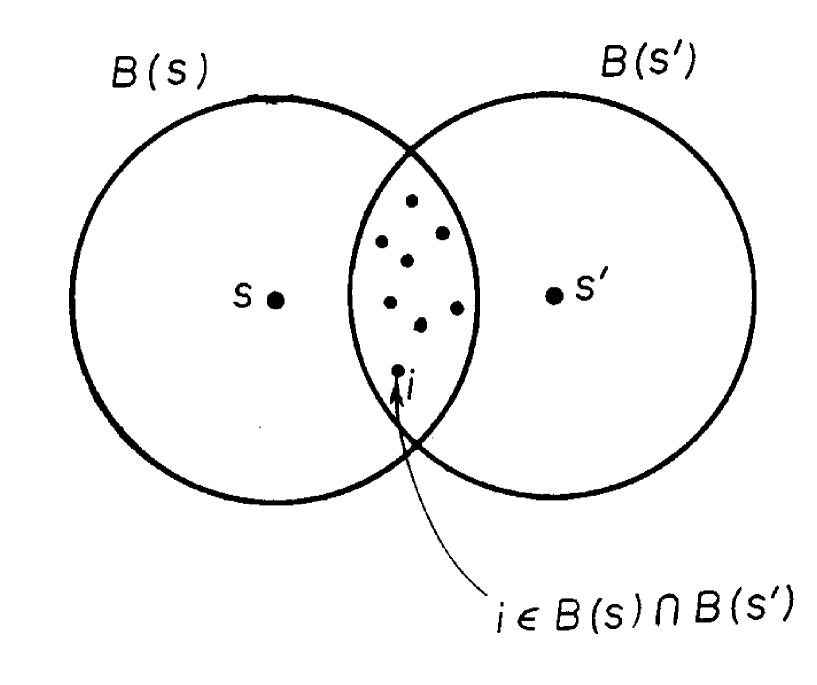
If the demon were, in the manner outlined above, to discover another neighbourhood $B(s^{\prime})$ of another site $s^{\prime}$ such that $B(s^{\mu})\cap B(s^{\prime})\neq\emptyset$, then he would hope to find among the (hopefully large) set of variables $\{\phi(i)\}$ for which $i\in B(s^{\mu})\cap B(s^{\prime})\neq\emptyset$ some that behave as link variables in the sense that they are transformed both by transformations (necessarily corresponding to the same representation) associated with the “site” $s^{\mu}$ and with transformations associated with the “site” $s^{\mu\prime}$ as indeed is characteristic of a link variable. Such a “link-like” configuration is illustrated in Figure 2.

Figure 2: If the number of fundamental space-time points $i\in\{j\}$ lying within $B(s^{\mu})\cap B(s^{\prime\mu})$ is large enough, then it becomes likely that there will be at least a single fundamental space-time point $i$ for which the corresponding field $\phi(i)$ transforms under the same representation of a common subgroup of $G(s^{\mu})$ and $G(s^{\prime\mu})$. Such a field variable will be said to have link-like behaviour.

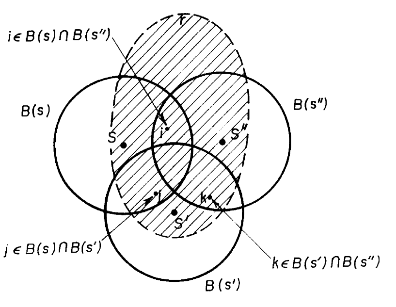
In order to have a microstate configuration that has a chance of giving rise to invariant terms of a (semi)local action contribution $S_{r}$, it is necessary that “link-like” variables are sufficiently profuse so as to ensure what we can call “plaquette-like” variables as a generic possibility: if “link-like” variables are sufficiently copious, one could hope to have part of the overlap of each of (at least) three “link-like” pairs of three gauge balls $B(s_{n}^{\mu})$ ($n\in\{1,2,3\}$) that intersect a (non)local action region $r$. Field variables from each of three such overlap regions (“link-like” variables - see last paragraph) of three gauge balls can be combined so as to simulate a “plaquette-like” variable (see Figure 3). If the coefficient of such a “plaquette variable” term in the action turns out to be large compared say to the coefficients of non-invariant contributions to $S_{r}$ (e.g., a “link-like” term), $S_{r}$ would be approximately invariant under the groups of (local) transformations $G(s_{n})$ ($n\in\{1,2,3\}$) associated with the three gauge balls $B(s_{n})$.

Figure 3: Consider three gauge balls $B(s^{\mu})$, $B(s^{\prime\mu})$ and $B(s^{\prime\prime\mu})$ for which the pair-wise overlap of each of three gauge ball pairs has a non-vanishing intersection with a (non)local action region $r$. Assume that the overlap of each such pair of gauge balls is populated by a number of fundamental space-time points $i$. Then it may be possible, for example, to find three fields $\phi(j)$, $\phi(k)$ and $\phi(i)$ - with let us say $j\in B(s^{\mu})\cap B(s^{\prime\mu})\cap r\neq\emptyset$, $k\in B(s^{\prime\mu})\cap B(s^{\prime\prime\mu})\cap r\neq\emptyset$ and $i\in B(s^{\prime\prime\mu})\cap B(s^{\mu})\cap r\neq\emptyset$ - such that all three fields transform as elements (in a common representation) of a subgroup common to $G(s^{\mu})$, $G(s^{\prime\mu})$ and $G(s^{\prime\prime\mu})$. This being the case, the composition $\phi(i)\cdot\phi(j)\cdot\phi(k)$ would be meaningful and would behave in a plaquette-like way in that a term of $S_{r}$ containing the trace of $\phi(i)\cdot\phi(j)\cdot\phi(k)$ would be approximately invariant under transformations corresponding to the above-mentioned common subgroup of $G(s^{\mu})$, $G(s^{\prime\mu})$ and $G(s^{\prime\prime\mu})$ associated with the three gauge balls $B(s^{\mu})$, $B(s^{\prime\mu})$ and $B(s^{\prime\prime\mu})$.

Figure 4: The 2-dimensional special case field theory glass is readily revealed by the demon as a priori being very nearly a gauge glass. Moving a point in the configuration space (16) along the orbit corresponding to the application of the elements of (17) to the fields $\phi$ at the four fundamental spacetime points $i\in\{I,II,III,IV\}$ lying within the gauge ball $B(s^{\mu})$ leave the action contributions $S_{r}=\beta ReU(\Box)+\kappa\sum_{\mbox{\begin{picture}(4.15,10.0)\put(0.0,3.0){\circle*{2.0}} \put(0.0,2.75){\line(1,0){7.0}} \put(7.3,3.0){\circle*{2.0}}\mbox{ } \end{picture} }\;\;\in r}ReU(\mbox{\begin{picture}(4.15,10.0)\put(0.0,3.0){\circle*{2.0}} \put(0.0,2.75){\line(1,0){7.0}} \put(7.3,3.0){\circle*{2.0}}\mbox{ } \end{picture} })$ (with $r\cap B(s^{\mu})\neq\emptyset$) approximately invariant if $\kappa$ is small. The index $r$ labels the non-local action regions (on which the $S_{r}$ are defined); these are drawn as broken-line rounded squares.

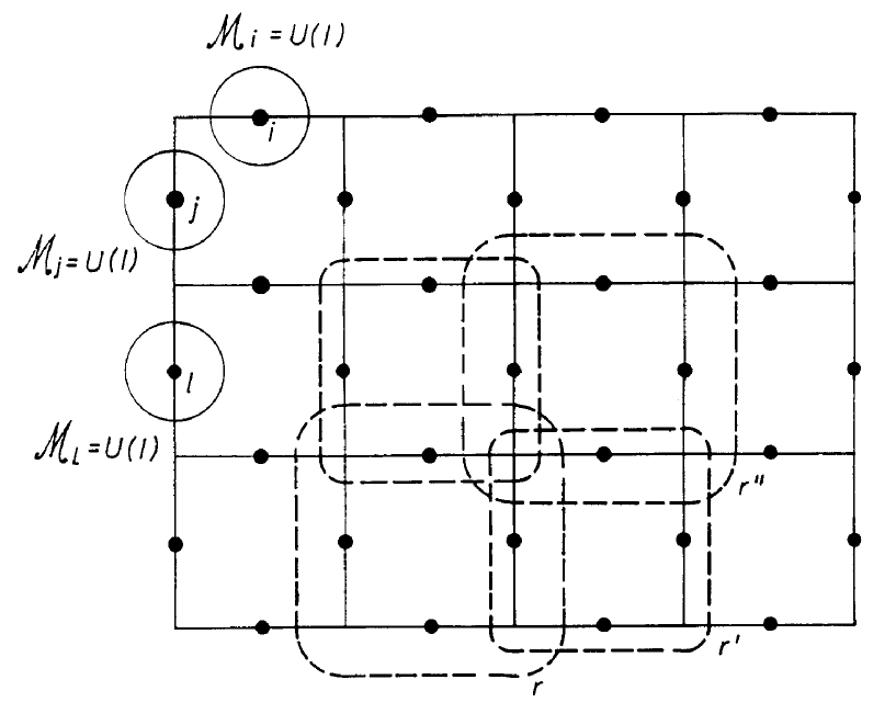
• In the “special case” field theory glass (really it turns out a priori to be close to being a gauge glass, but it is still illustrative to see how a demon might reveal this), a demon would eventually discover a gauge ball $B(s^{\mu})$ centred at an $s^{\mu}$ that coincides with a site of the hyper-cubic lattice (such a site is not one of the fundamental spacetime point $i\in\{j\}$ located at the centres of the links of the lattice). Let such a gauge ball $B(s^{\mu})$ contain the $i$’s located at the centres of the $2d$ ($d$ denotes dimension) links of the lattice emanating from the centre $s^{\mu}$ of $B(s^{\mu})$. In Figure 4 (with $d$=2), $B(s^{\mu})$ is indicated by the circle that contains four “fundamental space-time points” $i$ (labelled by the set $\{I,II,III,IV\}$) and has a non-vanishing intersection with four (overlapping) non-local action regions $r$ (corresponding to plaquettes containing four $i$’s). Each region $r$ such that $r\cap B(s^{\mu})\neq\emptyset$ contains two (adjacent) $i$’s of the four $i\in B(s^{\mu})=\{I,II,III,IV\}$. Let us make the (fortuitous) assumption that the action parameters $\{\beta,\kappa\}$ assigned to each non-local action region $r$ are (in addition to being identical for each region $r$) such that $\beta$ is large and $\kappa$ is small. Then the demon would, for example, observe large fluctuations on

  $$\times^{cart.\;prod}_{i\in B(s^{\mu})}{\cal M}_{i}=$$ (16)

  $${\cal M}_{i=I}\times{\cal M}_{i=II}\times{\cal M}_{i=III}\times{\cal M}_{i=IV}=U(1)_{i=I}\times U(1)_{i=II}\times U(1)_{i=III}\times U(1)_{i=IV}$$

  along an orbit coinciding with the elements of the group $G(s^{\mu})$ of symmetry operations

  $$G(s^{\mu})=\{(\exp(i\theta_{I}),\exp(i\theta_{II}),\exp(i\theta_{III}),\exp(i\theta_{IV}))|$$ (17)

  $$|\theta_{I}=-\theta_{II}=\theta_{II}=-\theta_{IV}\;[e^{i\theta_{I}}\in U(1)_{I}\wedge e^{i\theta_{II}}\in U(1)_{II}\wedge e^{i\theta_{III}}\in U(1)_{III}\wedge e^{i\theta_{IV}}\in U(1)_{IV}]\};$$

  i.e., $G(s^{\mu})$ is the group of (approximate) symmetry operations associated with the gauge ball $B(s^{\mu})$.

  For small $\kappa$ and large $\beta$, this group of transformations leaves the four non-local action contributions corresponding to the four regions $r$ that overlap $B(s^{\mu})$ approximately invariant.

2.4.1 The FNNS mechanism of exactification of an approximate gauge symmetry

The essential result of the FNNS mechanism is that the emergence of exact gauge symmetry in the long wavelength limit is, without fine-tuning, a generic possibility for a very broad class of field theories.

A prerequisite needed in order for the FNNS mechanism to work is an approximate gauge symmetry at say the fundamental scale. Then FNNS promises exact gauge symmetry (i.e. massless gauge bosons) in going to long wavelengths. Let us assume that such an approximate gauge symmetry has, in the manner sketched above, been found on a field theory glass - presumably from observing directions in configuration space along which there are large quantum fluctuations. Large fluctuations are expected in directions corresponding to orbits in configuration space along which the action $S$ is almost independent of the combinations of the $\phi(i)$ lying on such an orbit.

The validity of the FNNS statement is hard to see unless one uses the technique that the founders of FNNS used to construct the argument leading to the conclusion that the emergence of massless gauge bosons is a generic possibility for a broad class of fundamental scale field theories.

The technique consists in the (formal) rewriting of the (single) “God given” field $\phi$ in terms of new fictive fields $\phi_{h}(i)$ and $H(s^{\mu})$ defined respectively on fundamental space-time points $i$ and gauge ball centres $s^{\mu}$. These new variables are defined by

$$\phi(i)\stackrel{{\scriptstyle def}}{{=}}\phi_{h}^{H(s^{\mu})}(i)$$ (18)

With this formal replacement, we trivially acquire a formal symmetry under the transformations

$$\phi_{h}\rightarrow\phi_{h}^{\Omega}$$ (19)

$$H\rightarrow\Omega^{-1}H$$ (20)

inasmuch as transforming back and forth between $\phi_{h}$ and $H$ in this way that doesn’t change the $\phi$ field containing the physics; i.e.,

$$\phi=\phi_{h}^{H}\rightarrow(\phi_{h}^{\Omega})^{\Omega^{-1}H}=\phi_{h}^{H}=\phi$$ (21)

leaves $S[\phi_{h},H]\stackrel{{\scriptstyle def}}{{=}}S[\phi]$ invariant.

Having this formal symmetry also allows the freedom of choosing a gauge condition for the formal symmetry. The fact that these just formal manipulations will be done in a special way so as to make possible the analysis leading to the FNNS result in no way limits the (completely general) validity of the FNNS mechanism conclusion (i.e., photons without fine-tuning) because these formal manipulations are completely decoupled from the physics. In fact it is precisely because the formal manipulations of the $\phi_{h}$ and $H$ fields do not affect the physics that we can conclude that a physical result obtained using a very special manipulation of these fictive variables will remain valid in general (also when the fictive variables are manipulated away). The formal manipulations are however important in the sense that they reveal “hidden” physics that is otherwise not easy to see.

In the FNNS mechanism, the freedom to choose a gauge is used to rewrite the field $\phi(i)$ (with $i\in B(s^{\mu})$ say) as a site “$s$” associated part $H(s^{\mu})$ that is somehow common to the field variables $\phi(i)$ (with $i\in B(s^{\mu})$ and a part $\phi_{h}(i)$ that is the part of $\phi(i)$ that cannot be described by $H(s^{\mu})$. So the gauge choice that is made fixes $H$ to be the part of the $\phi(i)$ fluctuation pattern that for all $i\in B(s^{\mu})$ is common to the $\phi(i)$ field. Even though each field $\phi(i)$ takes values on a different target space ${\cal M}_{i}$, the pattern of fluctuation along different ${\cal M}_{i}$ can be correlated in the sense that in moving a point in configuration space along an orbit of large fluctuations results in changes in the various fields $\phi(i)$ that are correlated. For example, a common phase factor of fixed norm could be “factored out” of the fluctuation pattern of each $\phi(i)$ (with $i\in B(s^{\mu})$) and absorbed into the $H(s^{\mu})$ field defined on the centre of the gauge ball $B(s^{\mu})$. This renders the $H$ field a sort of non-linear Higgs field that fluctuates wildly in the target (configuration) space $\mbox{{\bf$\times$}}^{\mbox{{\tiny cart. prod.}}}_{i\in B(s^{\mu})}{\cal M}_{i}$. Since the $H(s^{\mu})$ field has the same value at all fundamental spacetime points $i\in B(s^{\mu})$ as a result of the choice of gauge, the action $S$ is roughly independent of $H$. Hence $H(s^{\mu})$ can have large fluctuations that can prevent the theory from Higgsing.

The remarkable result of the FNNS mechanism is that if it is possible to formally choose the gauge so that to a large extent the $\phi(i)$ field fluctuations come to reside in the site associated $H(s^{\mu})$ field, there is a generically good chance for having the $\phi_{h}$ field in a Coulomb phase without fine-tuning.

So far the $H$ field is not a proper Higgs field in that in general it will be a non-linear field that fluctuates on a non-convex (e.g. group) target space manifold. However, by block spinning the $H$ field, one can effectively introduce a new variable (not present on the group manifold) that allows the $H$ to effectively become linear. Block spinning essentially re-expresses the fluctuations in (the non-linear) $H$ on the target manifold in terms of this new variable that in effect fills out the non-convex target space manifold so as to form the convex closure of the latter. Of course the space in which the convex closure of the target space comes to reside must be postulated as being a reality. Such a constructed extension of the target space could be taken as the simplest possible space in which $H$ can be embedded linearly. For example, if a non-linear $H$ field takes values in a $U(1)$ target space, it could, by block spinning, become a normal linear Higgs field if $U(1)$ is first embedded in C. For large $H$ fluctuations, $H$ can even come to lie in the symmetric point of the convex envelope of the group manifold thereby attaining a vanishing value as indeed is also possible for a proper Higgs field. The founders of the FNNS mechanism[28] have demonstrated in a number of field theory models that there is a whole range of action parameters for which the fluctuations in $H$ are large enough to prevent the theory from being Higgsed and for which the correlations in the $\phi_{h}$ field are of sufficiently long range to yield a Coulomb phase.

• In the special case “field theory glass” for which there a priori is approximate $U(1)$ gauge symmetry, the derivation of the FNNS mechanism would first involve the introduction of the formal variables[27] $\phi_{h}(i)$ and $H(s^{\mu})$. The first is

  $$\phi_{h}(i)=U_{h}(\;\mbox{\begin{picture}(4.15,10.0)\put(0.0,3.0){\circle*{2.0}} \put(0.0,2.75){\line(1,0){7.0}} \put(7.3,3.0){\circle*{2.0}}\mbox{ } \end{picture} }^{\!\!\!\!\!\!\!s^{\mu}\;\;s^{\mu}+a\delta^{\mu}_{\nu}})\in U(1)\mbox{ defined on``links'' $i$ of lattice}$$ (22)

  ($a$ is the distance between adjacent gauge ball centres; e.g., the centre adjacent to that with coordinate $s^{\mu}$ in the the direction $\nu$ has coordinates $s^{\mu}+a\delta^{\mu}_{\nu}$).

  The second new variable is

  $$H(s^{\mu})=H(\mbox{\begin{picture}(4.15,4.0)\put(2.0,2.0){\circle*{2.0}} \end{picture} }^{\!\!\!\!\!s^{\mu}})\in U(1)\mbox{ defined on ``sites'' $s^{\mu}$ of lattice}.$$ (23)

  These two new variable are defined by

  $$\phi(i)=H^{-1}(\mbox{\begin{picture}(4.15,4.0)\put(2.0,2.0){\circle*{2.0}} \end{picture} }^{\!\!\!\!\!s^{\mu}})U_{h}(\;\mbox{\begin{picture}(4.15,10.0)\put(0.0,3.0){\circle*{2.0}} \put(0.0,2.75){\line(1,0){7.0}} \put(7.3,3.0){\circle*{2.0}}\mbox{ } \end{picture} }^{\!\!\!\!\!\!\!s^{\mu}\;\;s^{\mu}+a\delta^{\mu}_{\nu}})H(\mbox{\begin{picture}(4.15,4.0)\put(2.0,2.0){\circle*{2.0}} \end{picture} }^{\!\!\!\!\!s^{\mu}+a\delta^{\mu}_{\nu}}).$$ (24)

  The action

  $$S[U_{h},H]\stackrel{{\scriptstyle def}}{{=}}S[\phi(i)]=S[H^{-1}(\mbox{\begin{picture}(4.15,4.0)\put(2.0,2.0){\circle*{2.0}} \end{picture} }^{\!\!\!\!\!s^{\mu}})U_{h}(\;\mbox{\begin{picture}(4.15,10.0)\put(0.0,3.0){\circle*{2.0}} \put(0.0,2.75){\line(1,0){7.0}} \put(7.3,3.0){\circle*{2.0}}\mbox{ } \end{picture} }^{\!\!\!\!\!\!\!s^{\mu}\;\;s^{\mu}+a\delta^{\mu}_{\nu}})H(\mbox{\begin{picture}(4.15,4.0)\put(2.0,2.0){\circle*{2.0}} \end{picture} }^{\!\!\!\!\!s^{\mu}+a\delta^{\mu}_{\nu}})]$$ (25)

  is readily shown to be invariant under the following (formal) gauge transformations of the formal variables $U_{h}$ and $H$:

  $$U_{h}(\;\mbox{\begin{picture}(4.15,10.0)\put(0.0,3.0){\circle*{2.0}} \put(0.0,2.75){\line(1,0){7.0}} \put(7.3,3.0){\circle*{2.0}}\mbox{ } \end{picture} }^{\!\!\!\!\!\!\!s^{\mu}\;\;s^{\mu}+a\delta^{\mu}_{\nu}})\rightarrow\Lambda^{-1}(\mbox{\begin{picture}(4.15,4.0)\put(2.0,2.0){\circle*{2.0}} \end{picture} }^{\!\!\!\!\!s^{\mu}})U_{h}(\;\mbox{\begin{picture}(4.15,10.0)\put(0.0,3.0){\circle*{2.0}} \put(0.0,2.75){\line(1,0){7.0}} \put(7.3,3.0){\circle*{2.0}}\mbox{ } \end{picture} }^{\!\!\!\!\!\!\!s^{\mu}\;\;s^{\mu}+a\delta^{\mu}_{\nu}})\Lambda(\mbox{\begin{picture}(4.15,4.0)\put(2.0,2.0){\circle*{2.0}} \end{picture} }^{\!\!\!\!\!s^{\mu}+a\delta^{\mu}_{\nu}})$$ (26)

  $$H(\mbox{\begin{picture}(4.15,4.0)\put(2.0,2.0){\circle*{2.0}} \end{picture} }^{\!\!\!\!\!s^{\mu}})\rightarrow\Lambda^{-1}(\mbox{\begin{picture}(4.15,4.0)\put(2.0,2.0){\circle*{2.0}} \end{picture} }^{\!\!\!\!\!s^{\mu}})H(\mbox{\begin{picture}(4.15,4.0)\put(2.0,2.0){\circle*{2.0}} \end{picture} }^{\!\!\!\!\!s^{\mu}}).$$ (27)

  In terms of the new formal variables $U_{h}$ and $H$ the “semi-local” action contributions (14) (identical for each region $r$ in this very special case) each become

  $$S_{r}=S[U_{h},H]=\beta ReU_{h}(\Box)+\kappa\sum_{\;\mbox{\begin{picture}(4.15,10.0)\put(0.0,3.0){\circle*{2.0}} \put(0.0,2.75){\line(1,0){7.0}} \put(7.3,3.0){\circle*{2.0}}\mbox{ } \end{picture} }^{\!\!\!\!\!\!\!s^{\mu}\;\;s^{\mu}+a\delta^{\mu}_{\nu}}\in\Box}Re(H^{-1}(\mbox{\begin{picture}(4.15,4.0)\put(2.0,2.0){\circle*{2.0}} \end{picture} }^{\!\!\!\!\!s^{\mu}})U_{h}(\;\mbox{\begin{picture}(4.15,10.0)\put(0.0,3.0){\circle*{2.0}} \put(0.0,2.75){\line(1,0){7.0}} \put(7.3,3.0){\circle*{2.0}}\mbox{ } \end{picture} }^{\!\!\!\!\!\!\!s^{\mu}\;\;s^{\mu}+a\delta^{\mu}_{\nu}})H(\mbox{\begin{picture}(4.15,4.0)\put(2.0,2.0){\circle*{2.0}} \end{picture} }^{\!\!\!\!\!s^{\mu}+a\delta^{\mu}_{\nu}}).$$ (28)

  Let us now choose a gauge: e.g., $\prod_{\;\mbox{\begin{picture}(4.15,10.0)\put(0.0,3.0){\circle*{2.0}} \put(0.0,2.75){\line(1,0){7.0}} \put(7.3,3.0){\circle*{2.0}}\mbox{ } \end{picture} }^{\!\!\!\!\!\!\!x^{\mu}\;\;}\mbox{\tiny meeting at }\mbox{\begin{picture}(4.15,4.0)\put(2.0,2.0){\circle*{2.0}} \end{picture} }^{\!\!\!x^{\mu}}}U_{h}(\mbox{\begin{picture}(4.15,10.0)\put(0.0,3.0){\circle*{2.0}} \put(0.0,2.75){\line(1,0){7.0}} \put(7.3,3.0){\circle*{2.0}}\mbox{ } \end{picture} })=1$ (the lattice equivalent of the Lorentz gauge) or $U_{h}(\mbox{\begin{picture}(4.15,10.0)\put(0.0,3.0){\circle*{2.0}} \put(0.0,2.75){\line(1,0){7.0}} \put(7.3,3.0){\circle*{2.0}}\mbox{ } \end{picture} })=1$ for links in the direction $x^{0}$ (temporal gauge). Now, if $\beta$ is sufficiently large we will have

  $$U_{h}(\mbox{\begin{picture}(4.15,10.0)\put(0.0,3.0){\circle*{2.0}} \put(0.0,2.75){\line(1,0){7.0}} \put(7.3,3.0){\circle*{2.0}}\mbox{ } \end{picture} })\approx 1\mbox{ in the measure }{\cal D}U_{h}(\mbox{\begin{picture}(4.15,10.0)\put(0.0,3.0){\circle*{2.0}} \put(0.0,2.75){\line(1,0){7.0}} \put(7.3,3.0){\circle*{2.0}}\mbox{ } \end{picture} }){\cal D}H(\mbox{\begin{picture}(4.15,4.0)\put(2.0,2.0){\circle*{2.0}} \end{picture} })e^{S[U_{h},H]}/Z$$ (29)

  and the action (28) becomes

  $$S_{r}=S[U_{h}=1\mbox{ $\forall$ $\mbox{\begin{picture}(4.15,10.0)\put(0.0,3.0){\circle*{2.0}} \put(0.0,2.75){\line(1,0){7.0}} \put(7.3,3.0){\circle*{2.0}}\mbox{ } \end{picture} }$},H]=\sum\beta\mbox{\bf{1}}+\kappa\sum_{\;\mbox{\begin{picture}(4.15,10.0)\put(0.0,3.0){\circle*{2.0}} \put(0.0,2.75){\line(1,0){7.0}} \put(7.3,3.0){\circle*{2.0}}\mbox{ } \end{picture} }^{\!\!\!\!\!\!\!s^{\mu}\;\;s^{\mu}+a\delta^{\mu}_{\nu}}\in\Box}Re(H^{-1}(\mbox{\begin{picture}(4.15,4.0)\put(2.0,2.0){\circle*{2.0}} \end{picture} }^{\!\!\!\!\!s^{\mu}})H(\mbox{\begin{picture}(4.15,4.0)\put(2.0,2.0){\circle*{2.0}} \end{picture} }^{\!\!\!\!\!s^{\mu}+a\delta^{\mu}_{\nu}})$$ (30)

  $$\propto\kappa\sum_{\;\mbox{\begin{picture}(4.15,10.0)\put(0.0,3.0){\circle*{2.0}} \put(0.0,2.75){\line(1,0){7.0}} \put(7.3,3.0){\circle*{2.0}}\mbox{ } \end{picture} }^{\!\!\!\!\!\!\!s^{\mu}\;\;s^{\mu}+a\delta^{\mu}_{\nu}}}Re(H^{-1}(\mbox{\begin{picture}(4.15,4.0)\put(2.0,2.0){\circle*{2.0}} \end{picture} }^{\!\!\!\!\!s^{\mu}})H(\mbox{\begin{picture}(4.15,4.0)\put(2.0,2.0){\circle*{2.0}} \end{picture} }^{\!\!\!\!\!s^{\mu}+a\delta^{\mu}_{\nu}}).$$

  This is recognised as the “$x-y$”-model in 4-dimensions; from the decay correlation theorem it is known that there are no long range correlations for sufficiently small $\kappa$. Hence the Higgsed phase is avoided and for sufficiently large $\beta$ a Coulomb phase emerges complete with photons!

2.4.2 Relating microstates to macroscopic gauge fields

Starting with the microstate vacuum, we shall now demonstrate a procedure for setting up a macroscopic gauge potential $A^{a}_{\mu}(y_{I})$. This will be done by transforming the field variables $\phi(i)$ at the fundamental space-time points $i\in\{j\}$ using the local microlevel transformations $\Lambda(s^{\mu})\in G(s^{\mu})$ that are associated with the gauge balls $B(s^{\mu})$ within which a fundamental space-time point $i$ (corresponding to $\phi(i)$) lies. We shall also demonstrate that there is a microstate transformation that corresponds to a pure gauge transformation of a macroscopic $A^{a}_{\mu}$ field. Recall that a microstate is specified by a point in $\mbox{{\bf$\times$}}^{\mbox{{\tiny cart. prod.}}}_{i\in\{j\}}{\cal M}_{i}$ (i.e., configuration space). Such a point corresponds to a value of $\phi(i)$ for each $i\in\{j\}$ where $\{j\}$ denotes the set of fundamental space-time sites.

We begin by choosing an (arbitrary) partition of the set of fundamental space-time sites $\{j\}$ in the field theory glass into a set $\{{\cal P}_{y^{\mu}_{J}}\}$ of non-overlapping cells ${\cal P}_{y^{\mu}_{I}}\in\{{\cal P}_{y^{\mu}_{J}}\}$ in such a way that every fundamental space-time point $i$ lies in one and only one cell ${\cal P}_{y^{\mu}_{I}}$. Cells are labelled by the coordinate $y^{\mu}_{I}$ that by definition lies within the cell ${\cal P}_{y^{\mu}_{I}}$. We require that a cell is small to a degree sufficient to validate the assumption that the variation of $A^{a}_{\mu}$ within any cell is negligible.

Any fundamental site $i\in\{j\}$ will always fall within a unique cell of the partition - let us say that $i$ falls within the cell ${\cal P}_{y^{\mu}_{J}}$:

$$i\in{\cal P}_{y^{\mu}_{J}}\in\{{\cal P}_{y^{\mu}_{I}}\}.$$ (31)

In general, $i$ will also belong to a set of gauge balls:

$$\{B(s^{\prime\mu})|i\in B(s^{\prime\mu})\}.$$ (32)

The set (32) can be empty or contain a number of gauge balls depending on the density of gauge balls.

Choose now some cell ${\cal P}_{y^{\mu}_{J}}$ and consider the following subset of the set $\{j\}$ of fundamental space-time points:

$$\{k|k\in\{j\}\wedge k\in{\cal P}_{y^{\mu}_{J}}\wedge k\in B(s^{\prime\mu})\}.$$ (33)

Now let each fundamental space-time point $k$ belonging to the set (33) be transformed according to

$$\lambda^{a}(s^{\prime\mu})=A^{a}_{\mu}(y_{J})(s^{\prime\mu}-y^{\mu}_{J})+c(y_{J}).$$ (34)

where $A^{a}_{\mu}$ is the macroscopic field that we want to set up at $y^{\mu}_{J}$ and $s^{\prime\mu}$ labels the gauge balls $B(s^{\prime\mu})$ for which $B(s^{\prime\mu})\cap{\cal P}_{y^{\mu}_{J}}\neq\emptyset$. The $c(y^{\mu}_{J})$ is a quantity depending only on $y^{\mu}_{J}$ that without loss of generality can be set to zero (because we assume the theory is not Higgsed). This $\lambda^{a}(s^{\prime\mu})$ is the generator of an element $\Lambda(s^{\prime\mu})\in G(s^{\prime\mu})$

$$\Lambda(s^{\prime\mu})=\exp(i\lambda^{a}(s^{\prime\mu})\tau^{a}/2)$$ (35)

that transforms all $\phi(i)$ with $i\in B(s^{\prime\mu})$. Recall that $G(s^{\prime\mu})$ is the set of symmetry operations associated with the gauge ball $B(s^{\prime\mu})$ such that each element of $\Lambda(s^{\mu})\in G(s^{\mu})$ transforms all the $\phi(i)$ corresponding to fundamental spacetime points $i$ within the gauge-ball $B(s^{\mu})$. These transformations are such that action contributions $S_{r}$ associated with regions $r\in\{r^{\prime}|r^{\prime}\cap B(s^{\mu})\neq\emptyset\}$ remain approximately invariant if and only if all $k\in B(s^{\mu})$ are transformed by the same element $\Lambda(s^{\mu})\in G(s^{\mu})$.

In general this is not the case. From (34) it is seen that fundamental spacetime points get transformed by transformations that depend on the cell ${\cal P}_{y^{\mu}_{J}}$ (labelled by $y^{\mu}_{J}$) within which these points lie. The important point is that if a gauge ball $B(s^{\mu})$ falls within more than one cell, then $k\in B(s^{\mu})$ get transformed by (different) $\Lambda(s^{\mu})\in G(s^{\mu})$ according to which cell $k$ belongs. If an action region $r$ (corresponding to an $S_{r}$ that depends only on the field variables $\phi(i)$ with $i\in r$) contains fundamental spacetime points lying within the same gauge ball $B(s^{\mu})$ but different cells of the partition, then fields $\phi$ at the fundamental spacetime points in different cells get transformed by different elements $\Lambda(s^{\mu})\in G(s^{\mu})$. The result is an operation under which $S_{r}$ is not invariant. Such operations can be used to alter the microstate vacuum so as to set up any prescribed macroscopic $A_{a}^{\mu}(y_{J})$ corresponding to a field configuration with non-vanishing $F^{\mu\nu}$.

By way of example, consider the case where the two field variables $\phi(l)$ and $\phi(m)$ with $l,m\in B(s^{\mu})$ fall respectively into two different cells ${\cal P}_{y^{\mu}_{I}}$ and ${\cal P}_{y^{\mu}_{K}}$ of the partition $\{{\cal P}_{y^{\mu}_{J}}\}$. Then $\phi_{l}$ and $\phi_{m}$ are transformed by different group elements of $G(s^{\mu})$: the field variable $\phi_{l}$ is transformed by the element $\Lambda(s^{\mu})\in G(s^{\mu})$ generated by the Lie algebra element $\lambda(s^{\mu})=A(y_{I})(s^{\mu}-y^{\mu}_{I})$ while $\phi_{m}$ is transformed by the element of $G(s^{\mu})$ generated by $\lambda(s^{\mu})=A(y_{K})(s^{\mu}-y^{\mu}_{K})$. Were the field variables $\phi_{l}$ and $\phi_{m}$ “links” of a plaquette lying in in some local action contribution $S_{r}$, the corresponding plaquette term of $S_{r}$ would not be invariant under the modification of the microstate vacuum outlined above. Indeed, such a modification would in general lead to a non-vanishing curvature for such a plaquette.

In the special case that a gauge ball $B(s^{\mu})$ lies entirely within a single cell ${\cal P}_{y^{\mu}_{I}}$ of the partition $\{{\cal P}_{y^{\mu}_{J}}\}$, the fundamental spacetime points in this gauge ball are all transformed by the same element

$$\Lambda(s^{\mu})=\exp(iA^{a}_{\mu}(y_{J})(s^{\mu}-y^{\mu}_{J})\tau^{a}/2)\in G(s^{\mu})$$ (36)

which just leaves us in the vacuum. This will be seen to correspond simply to a gauge transformation of the microstate vacuum.

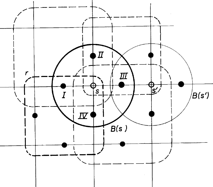
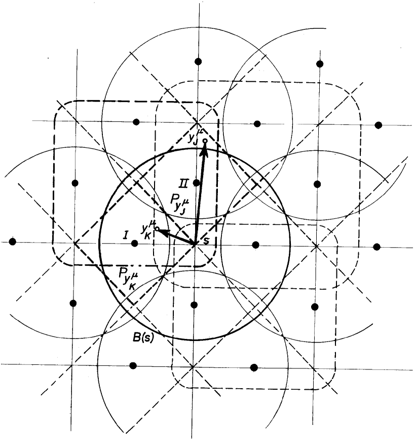
• In the special case “field theory glass” (i.e., in the case where we almost have a gauge glass from the start), let the partition ${\cal P}_{\{y^{\mu}_{J}\}}$ be the squares formed by the dashed diagonal lines in Figure 5. Assume that the points $y^{\mu}_{K}$ and $y^{\mu}_{J}$ are arbitrarily situated in respectively the cells ${\cal P}_{y^{\mu}_{K}}$ and ${\cal P}_{y^{\mu}_{J}}$. Then the field $\phi(I)$ at the fundamental spacetime point I is transformed by the element $\Lambda(s^{\mu})=\exp(iA^{\mu}(y_{K})(s^{\mu}-y^{\mu}_{K}))\in G(s^{\mu})$ corresponding to the setup of the field value $A^{\mu}(y_{K})$ at $y^{\mu}_{K}$ in ${\cal P}_{y^{\mu}_{K}}$. In an analogous fashion, the field $\phi(II)$ at the fundamental spacetime point II is transformed by the element $\Lambda^{\prime}(s^{\mu})=\exp(iA^{\mu}(y_{II})(s^{\mu}-y^{\mu}_{II}))\in G(s^{\mu})$ corresponding to the set-up of the field value $A^{\mu}(y_{II})$ at $y^{\mu}_{II}\in{\cal P}_{y^{\mu}_{II}}$. The essential point is that $\phi(I)$ and $\phi(II)$ are transformed by different elements $\Lambda(s^{\mu})$ and $\Lambda^{\prime}(s^{\mu})$ of the symmetry group $G(s^{\mu})$ associated with the same gauge ball (namely the gauge ball containing both the fundamental spacetime points $I$ and $II$. The (semi)local action contribution $S_{r}$ defined on the (non)local region $r$ within which $I$ and $II$ lie is approximately invariant when the fields at the fundamental spacetime points (within any gauge ball $B(s^{\mu})$ with $B(s^{\mu})\cap r\neq\emptyset$) are all transformed by the same element of the gauge group $G(s^{\mu})$. But this is in general not true when such fields $\phi(I)$ and $\phi(II)$ are transformed by different elements of $G(s^{\mu})$. It is precisely this situation - i.e., different fields $\phi(I)$ and $\phi(II)$ corresponding to fundamental spacetime points within the same gauge ball that are transformed by different elements of $G(s^{\mu})$ - that is needed in order to set up macroscopic fields $A_{\mu}$ of any desired curvature.

Figure 5: In the figure, the chosen partition of the special field theory glass is shown as the diagonal broken-line grid; ${\cal P}_{y^{\mu}_{K}}$ and ${\cal P}_{y^{\mu}_{J}}$ denote cells of this partition containing respectively the (arbitrarily placed) points $y^{\mu}_{K}$ and $y^{\mu}_{J}$. Consider by way of example the fields $\phi(I)$ and $\phi(II)$ at the fundamental spacetime points $I$ and $II$ that both fall within the same gauge ball $B(s^{\mu})$. As $\phi(I)$ (with $I\in{\cal P}_{y^{\mu}_{K}}$) and $\phi(II)$ (with $I\in{\cal P}_{y^{\mu}_{J}}$) are transformed by the different elements $\exp(A_{\mu}(y_{K})(s^{\mu}-y^{\mu}_{K}))$ and $\exp(A_{\mu}(y_{J})(s^{\mu}-y^{\mu}_{J}))$, of $G(s^{\mu})$, we can choose these elements so as to correspond to mutually independent fields $A_{\mu}(y_{K})(s^{\mu}-y^{\mu}_{K})$ and $A_{\mu}(y_{J})(s^{\mu}-y^{\mu}_{J})$ of any desired values.

It has been demonstrated that any macroscopic $A_{\mu}$ field can be set up by a modification of the fields $\phi_{k}$ of the (quenched) microstate vacuum using (local) transformations from (approximate) symmetry groups $G(s^{\mu})$ associated with the different gauge balls $B(s^{\mu})$ of the overlapping system of gauge balls that contain the fundamental space-time sites $k$ at which the fields $\phi(k)$ are defined.

It is important to see that there is also a correspondence between a usual gauge transformation of a macroscopic gauge field $A_{\mu}$ and a modification of the microstate vacuum that corresponds to a (pure) gauge transformation. To see this, consider a usual gauge transformation of a macroscopic gauge field $A_{\mu}\stackrel{{\scriptstyle def}}{{=}}A_{\mu}^{a}\tau^{a}/2$:

$$A_{\mu}(x)\rightarrow A_{\mu}(x)^{\Omega(x)}\stackrel{{\scriptstyle def}}{{=}}\Omega^{-1}(x)A_{\mu}(x)\Omega(x)+i\Omega^{-1}(x)\partial_{\mu}\Omega(x)$$ (37)

We want to see the relation between two microstate transformations leading to two macroscopic gauge fields that are related by (37). In doing this, it is easier to work with the group elements $\Lambda(s^{\mu})\in G(s^{\mu})$ that transform the microstate in the desired way rather than the Lie algebra elements $\lambda(s^{\mu})$ that generates this transformation.

In setting up some macroscopic $A_{\mu}$ field by performing transformations of microstates, we can deal with one cell at a time. Consider therefore some cell ${\cal P}_{y^{\mu}_{J}}$; this cell ${\cal P}_{y^{\mu}_{J}}$ generally contains some subset of the set $\{j\}$ of fundamental spacetime points:

$$\{k|k\in\{j\}\wedge k\in{\cal P}_{y^{\mu}_{J}}\}$$ (38)

and intersects some set of gauge balls

$$\{B(s^{\prime\mu})|B(s^{\prime\mu})\cap{\cal P}_{y^{\mu}_{J}}\neq\emptyset\}.$$ (39)

For each of the gauge balls $B(s^{\mu})$ in the set (39) we perform the microstate transformation

$$\Lambda^{A_{\mu}}_{y^{\nu}_{J}}(s^{\nu})\stackrel{{\scriptstyle def}}{{=}}P\left(\exp\left(i\int_{y^{\nu}_{J}}^{s^{\nu}}A_{\mu}(x^{\nu})dx^{\mu}\right)\right)\in G(s^{\nu})$$ (40)

that is determined by the $A_{\mu}$ field that we want to set up (hence the superscript “$A_{\mu}$” on $\Lambda^{A_{\mu}}_{y^{\nu}_{J}}(s^{\nu})$). The subscript indicates that this is a (microstate) transformation of the fields $\phi(k)$ with $k\in{\cal P}_{y^{\nu}_{J}}$. The argument $s^{\nu}$ indicates that the fields $\phi(i)$ that get transformed are those associated with $i$ lying in $B(s^{\mu})\cap{\cal P}_{y^{\mu}_{J}}$. The “$P$” preceding the integral indicates that a path ordered product is to be taken.

The number of such transformations performed in each cell in setting up a given macroscopic $A_{\mu}$ field is just the number of elements in the set (39); a field $\phi(j)$ at a fundamental spacetime point $j$ contained in the set (38) gets transformed once for each gauge ball of the set (39) within which $j$ lies.

Now if we want to set up the field that has been gauge transformed according to (37)), then we want to use the microstate transformations (40) after these have been transformed according to

$$\Lambda^{A_{\mu}}_{y^{\nu}_{J}}(s^{\nu})\rightarrow\Lambda^{A_{\mu}^{\Omega}}{y^{\nu}_{J}}(s^{\nu})=\Omega^{-1}(s^{\nu})\Lambda^{A_{\mu}}_{y^{\nu}_{J}}(s^{\nu})\Omega(y^{\nu}_{J})\;\;(\Omega\in G(s^{\nu})).$$ (41)

In order to establish that this corresponds to a pure gauge transformation of the microstate vacuum, we need to show that all the $\phi(k)$ corresponding to $k$ lying within a given gauge ball $B(s^{\mu})$ get transformed by only one element $\Lambda(s^{\mu})\in G(s^{\mu})$ of the group $G(s^{\mu})$ associated with this gauge ball. This is the opposite of the situation needed to set up an $A_{\mu}$ in general (with non-vanishing curvature): recall from above that in setting up an $A_{\mu}$ field in general, it was essential that the fields $\phi(k)$ corresponding to $k\in B(s^{\mu})$ transform in a cell dependent way. This being the case, a gauge ball intersected by more than one cell could have fields $\phi(k)$ and $\phi(l)$ (corresponding to fundamental spacetime points in different cells) that would be transformed by different elements of $G(s^{\mu})$ with the consequence that $A_{\mu}$ fields with non-vanishing (or modified) $F_{\mu\nu}$ could be set up. In order to show that $\Lambda^{A_{\mu}}_{y^{\nu}_{J}}$ and $\Lambda^{A^{\Omega(x)}_{\mu}}_{y^{\nu}_{J}}$ both set up macroscopic $A_{\mu}$ fields having the same $F_{\mu\nu}$ (i.e., macroscopic fields related by a pure gauge transformation), we need to show that the transformation (41) takes place in a cell independent way. Looking at (41), this would at first glance seem difficult because (41) involves a transformation $\Omega(y^{\mu}_{J})$ with a cell dependent argument $y_{J}^{\mu}$: while it is true that in (41) both $\Omega(y_{J}^{\nu})$ and $\Omega(s^{\nu})$ are elements of $G(s^{\nu})$, they are not the the same element of $G(s^{\nu})$. The element $\Omega(y_{J}^{\nu})\in G(s^{\nu})$ is obtained by the parallel transport of $G(s^{\nu})$ from $s^{\nu}$ to $y_{J}^{\nu}$ along $y_{J}^{\nu}-s^{\nu}$ using (40).

But now we make use of the fact that we are assuming that our field theory glass is un-Higgsed. This means that two vacua that are related by a global gauge transformation are really exactly the same vacuum. In particular, we can do global transformations for each cell; when we get to the cell ${\cal P}_{y_{J}^{\mu}}$, we perform the global gauge transformation $\Omega(y^{\mu}_{J})^{-1}$ on all gauge balls. Letting $\Omega^{-1}(y_{J}^{\mu})$ act on (41) from the right yields a transformation

$$\Lambda^{A^{\Omega(x)}_{\mu}}_{y^{\nu}_{J}}\Omega(y^{\nu}_{J})^{-1}=\Omega^{-1}(s^{\nu})\Lambda^{A_{\mu}}_{y^{\nu}_{J}}(s^{\nu})$$ (42)

of the same vacuum that is completely equivalent to (41). The right-hand side of (42) is a single element of $G(s^{\nu})$ namely that obtained as the group product of $\Omega^{-1}(s^{\nu})\in G(s^{\nu})$ and the transformation $\Lambda^{A_{\mu}}_{y^{\nu}_{J}}(s^{\nu})\in G(s^{\nu})$ that sets up the macroscopic field $A_{\mu}$ before it is subjected to the gauge transformation (37). The important point is that the transformation (42) depends only on $s^{\nu}$ and not on the cell ${\cal P}_{y^{\nu}_{J}}$.

Repeating this procedure for each cell ${\cal P}_{y_{J}^{\mu}}$ of the partition, it is seen that the net result is that the fields $\phi(k)$ for $k\in B(s^{\mu})$ always get transformed by the same element $\Lambda(s^{\mu})\in G(s^{\mu})$ even if such a gauge ball lies in more than one cell of the partition. Accordingly, we can conclude that the application of the microstate transformations $\Lambda^{A_{\mu}}_{J}$ and $\Lambda^{A^{\Omega(x)}_{\mu}}_{J}$ to the microstate vacuum sets up respectively macroscopic fields $A_{\mu}(x)$ and $A_{\mu}^{\Omega(x)}(x)$ that are related to each other by a pure gauge transformation. This was what we set out to show.

2.4.3 Multiple point criticality from a field theory glass

We have demonstrated a procedure for setting up a macroscopic $A_{\mu}$ field locally in space-time regions delineated by gauge balls $B(s^{\mu})$ using the gauge ball-associated group $G(s^{\mu})$ of (approximate) symmetry transformations $\Lambda(s^{\mu})\in G(s^{\mu})$ to modify the microstate vacuum $\Phi_{\{i\}}$ at space-time points $i$ lying within the gauge ball $B(s^{\mu})$. More specifically, it was seen that in order to set up a gauge field having non-vanishing curvature, it is necessary that a gauge-ball $B(s^{\mu})$ be intersected by more than one cell of an (arbitrary) partition $\{{\cal P}_{y^{\mu}_{J}}\}$ of the fundamental set of space-time sites $\{i\}$. This being the case, it is generically possible to find two fundamental space-time sites $j$ and $k$ such that even when $j,k\in B(s^{\mu})$, the associated $\phi_{j}$ and $\phi_{k}$ get transformed by different group elements of the set of gauge transformations $G(s^{\mu})$ that are approximate symmetries of (non)local action contributions $S_{r}$ for which $r\cap B(s^{\mu})\neq\emptyset$. This will generally be the case when $j$ and $k$ belong to different cells ${\cal P}_{y^{\mu}_{I}}$ and ${\cal P}_{y^{\mu}_{L}}$ of the partition $\{{\cal P}_{y^{\mu}_{J}}\}$ in which case the fields $\phi_{j}$ and $\phi_{k}$ transform according to $\phi_{j}\rightarrow\exp(iA_{\mu}(y_{I})(s^{\mu}-y^{\mu}_{I}))\phi_{j}$ and $\phi_{k}\rightarrow\exp(iA_{\mu}(y_{L})(s^{\mu}-y_{L}^{\mu}))\phi_{k}$. In general, such a combination of transformations does not coincide with just a single element $\Lambda(s^{\mu})$ of the set $G(s^{\mu})$ of (approximate) symmetries of the $S_{r}$ for which $r\cap B(s^{\mu})\neq\emptyset$.

An implicit assumption in this procedure is that there are microstate field variable degrees of freedom $\phi_{i}$ that can be modified non-trivially under the transformations of the various $G(s^{\mu})$ associated with the various gauge balls $B(s^{\mu})$; otherwise the action can only remain constant. The point is that a continuum limit $\frac{1}{g^{2}}$ must stem from a sum of contributions coming from microstate configurations that can represent a $gA^{\mu}$ field. An essential prerequisite for setting up such macroscopic $gA_{\mu}$ fields in the manner outlined above is that there is a sufficient density of sites among the set $\{i\}$ of fundamental space-time sites at which the associated field variables $\phi(i)$ transform non-trivially under the approximate symmetry group $G(s^{\mu})$ associated with some gauge ball $B(s^{\mu})$.

When the demon succeeds in finding a set of transformations $\Lambda(s^{\mu})\in G(s^{\mu})$ where $G(s^{\mu})$ is a group associated with a gauge ball $B(s^{\mu})$, he was presumably helped by the observation of large quantum fluctuations along a (closed) orbit $ORB_{large\;fluc\;in\mbox{{\bf$\times$}}^{\mbox{{\tiny cart. prod.}}}_{i\in B(s^{\mu})}{\cal M}_{i}}\subset\mbox{{\bf$\times$}}^{\mbox{{\tiny cart. prod.}}}_{i\in B(s^{\mu})}{\cal M}_{i}$ (or a set of “parallel” orbits corresponding to different choices of (distant) physical boundary conditions) on the manifold $\mbox{{\bf$\times$}}^{\mbox{{\tiny cart. prod.}}}_{i\in B(s^{\mu})}{\cal M}_{i}$. That large fluctuations are allowed along these orbits is a indication that the action is almost constant along such orbits. For a given set of distant boundary conditions, the different points on $ORB_{large\;fluc\;in\mbox{{\bf$\times$}}^{\mbox{{\tiny cart. prod.}}}_{i\in B(s^{\mu})}{\cal M}_{i}}{\cal M}_{i}$ are related by the transformations $\Lambda(s^{\mu})\in G(s^{\mu})$.

Along such orbits, the distributions of target space values taken by the fields $\phi(i)$ are such that there are correlations in the way that the values assumed by these $\phi$ change. In other words, in moving the configuration space point along such an orbit, we expect that the different fields $\phi(i)$ (with $i\in B(s^{\mu})$) will change in a correlated way. This behaviour would also follow from the properties that we expect to be characteristic of such an orbit. Recall that having such an orbit is presumably tantamount to having found a subset of the set of possible field variable combinations $\phi:\{i\}\cap B(s^{\mu})\rightarrow\mbox{{\bf$\times$}}^{\mbox{{\tiny cart. prod.}}}_{i\in B(s^{\mu})}{\cal M}_{i}$ for which the $S_{r}$ (with $r\cap B(s^{\mu})\neq\emptyset$) are invariant and for which the Cartesian product structure of $\mbox{{\bf$\times$}}^{\mbox{{\tiny cart. prod.}}}_{i\in B(s^{\mu})}{\cal M}_{i}$ is intact. If these properties are fulfilled, there will be points along such a configuration space orbit that can be transformed into each other under the action of a group (see footnote on page 1). The effect of such group operations is to permute points in configuration space (on the orbit) that correspond to whole sets of values of the $\phi(i)$ on such an orbit. This permutation symmetry is in itself an expression of the correlated way in which the $\phi(i)$ change when a point in configuration space is moved along such an orbit $ORB_{large\;fluc\;in\mbox{{\bf$\times$}}^{\mbox{{\tiny cart. prod.}}}_{i\in B(s^{\mu})}{\cal M}_{i}}\subset\mbox{{\bf$\times$}}^{\mbox{{\tiny cart. prod.}}}_{i\in B(s^{\mu})}{\cal M}_{i}$.

We seek now to extract the common variation in the various $\phi(i)$ field combinations corresponding to permutations (i.e., displacements) of configuration points on such orbits. The idea is to incorporate this common movement of the $\phi(i)$’s into a fictive (formal) field variable $H(s^{\mu})$ that takes values in $G(s^{\mu})$. The fictive variable $H(s^{\mu})$ (that maps sites $s$ into configuration space) is defined together with another fictive variable $\phi_{h}(i)$ by

$$\phi(i)=\phi_{h}^{H(s^{\mu})}(i).$$ (43)

This completely formal replacement of a “God-given” variable by a combination of formal variables is reminiscent of the technique used in establishing the FNNS Theorem. Recall that the physical content of the FNNS Theorem is revealed by formal manipulations un-coupled to the physics of a field theory but which are extremely useful in exposing the validity of the physical content of the FNNS mechanism. That real physics can be uncovered using an analysis with fictive variables relies on the fact that such formal operations cannot modify the physical content of a theory. However if such formal manipulations help to reveal real physics, such real physics is still there even when such fictive variables are manipulated in some other way (and in particular when such fictive variables are completely manipulated away).

The argumentation to be given below suggests that MPC actually results from a rather precise compromise between competing behaviour the one extreme of which favours the avoidance of a Higgs phase by having confinement while the other extreme favours the avoidance of confinement by having a Higgsed phase. It will be argued that at the multiple point, the chances of avoiding confinement and Higgsing are best.

In the spirit of the FNNS fictive variable technique, the second new field variable $\phi_{h}(i)$ corresponds to the part of the fluctuation pattern of the $\phi(i)$ (with $i\in B(s^{\mu})$) that remains after “correlated variations” in the values assumed by the variables $\phi(i)$ have been absorbed into the new field $H(s^{\mu})$ defined at the gauge ball centre $s$. This amounts to choosing a gauge for the formal symmetry that comes from introducing fictive variables in such a way that the $\phi(i)_{h}$ have smaller fluctuations than the original fields $\phi(i)$.

Now recall that the orbit $ORB_{large\;fluc\;in\mbox{{\bf$\times$}}^{\mbox{{\tiny cart. prod.}}}_{i\in B(s^{\mu})}{\cal M}_{i}}\subset\mbox{{\bf$\times$}}^{\mbox{{\tiny cart. prod.}}}_{i\in B(s^{\mu})}{\cal M}_{i}$ corresponds to transformations that are only approximately symmetries of the action contributions $S_{r}$ corresponding to the (non)local regions $r$ that overlap the gauge ball $B(s^{\mu})$. There can be small imperfections - i.e., points on the orbit $ORB_{large\;fluc\;in\mbox{{\bf$\times$}}^{\mbox{{\tiny cart. prod.}}}_{i\in B(s^{\mu})}{\cal M}_{i}}\subset\mbox{{\bf$\times$}}^{\mbox{{\tiny cart. prod.}}}_{i\in B(s^{\mu})}{\cal M}_{i}$ corresponding to (shallow) relative minima in one or more of the (coupled) $S_{r}$ corresponding to (non)local regions $r$ that overlap $B(s^{\mu})$.

Having a shallow minimum in an $S_{r}$ - coupled to other (semi)local action contributions $S_{r^{\prime}}$, $S_{r^{\prime\prime}}$, $\dots$ due to the overlap of (non)local regions $r$, $r^{\prime}$, $r^{\prime\prime}$, $\dots$ with $B(s^{\mu})$ - makes for the risk of an alignment of the field $H$ at $s$ that can become correlated with $H$ at other points $s^{\prime}$, $s^{\prime\prime}$, $\dots$ separated from $s$ by distances large enough to lead to Higgsing.

However, Higgsing can be rendered less likely if the fluctuations in $\phi_{h}(i)$ are large enough (corresponding to not having a coupling for the field $\phi_{h}(i)$ that is too weak) to inhibit such correlations in $H$ over large distances. Presumably, the weaker the coupling of the $\phi(i)$, the more of the original fluctuation pattern is common to the $\phi(i)$ (with $i\in B(s^{\mu})$) and therefore incorporated into the $H(s^{\mu})$ field. The remainder of the fluctuation pattern of the $\phi(i)$ fields - the incoherent part that cannot be put into the $H(s^{\mu})$ field - resides in the $\phi_{h}(i)$ and in a statistical sense at least can help to drown out imperfections in the approximate symmetries under the group $G(s^{\mu})$ that could lead to Higgsing.

But if the coupling is too strong, the fluctuations in the (new) variables $\phi_{h}(i)$ are so large that we get confinement of these degrees of freedom (and at the same time more effectively reduce the risk of Higgsing of the $H$-fields).

What we want is long range correlations for the degrees of freedom corresponding to the new variables $\phi_{h}(i)$ while at the same avoiding a Higgsing of the new variable $H(s^{\mu})$. This is the compromise that we claim is sought out by the MPCP.

The weaker the coupling for the variables $\phi_{h}(i)$ - (corresponding to smaller fluctuations in $\phi_{h}(i)$ that accordingly are less effective in preventing correlations in the $H$ field over long distances) - the more near perfect must be the “approximate” gauge symmetries found by the demon if the small uncorrelated fluctuations in $\phi_{h}(i)$ (with $i\in B(s^{\mu})$) are - at least statistically speaking - to be effective in reducing correlations in the $H$-field over distances that can lead to Higgsing.

Consider a gauge ball $B(s^{\mu})$. We want to define a quantity that expresses the amount by which a group of transformations $G(s^{\mu})$ associated with this gauge ball $B(s^{\mu})$ deviates from being a perfect symmetry. Such a quantity, denoted by $\Delta_{dev}$, is considered for each local action contribution $S_{r}$ for which the corresponding (non)local region $r$ (containing all the field variables $\phi_{i}$ on which $S_{r}$ depends non-trivially) is such that $r\cap B(s^{\mu})\neq\emptyset$. This quantity $\Delta_{dev}$ is defined by

$$\Delta_{dev}(G(s^{\mu}))=\stackrel{{\scriptstyle max}}{{\tiny over\;r}}||S_{r}[\phi^{\Lambda}]-\langle S_{r}[\phi^{\Lambda}]\rangle_{\Lambda\in G(s^{\mu})}||\mbox{ for }r\cap B(s^{\mu})\neq\emptyset\mbox{ and }\Lambda(s^{\mu})\in G(s^{\mu}).$$ (44)

According to the argumentation above, the quantity $\Delta_{dev}(G(s^{\mu}))$ must be smaller the larger the inverse squared coupling if the risk for Higgsing due to deviations from perfect symmetry is not to increase. We can express this requirement by an inequality that must be satisfied:

$$\Delta_{dev}(G(s^{\mu}))\leq f(\frac{1}{g^{2}})$$ (45)

where $f(\frac{1}{g^{2}})$ is a monotonically decreasing function of $\frac{1}{g^{2}}$ and $\Delta_{dev}(G(s^{\mu}))$ is given by (44).

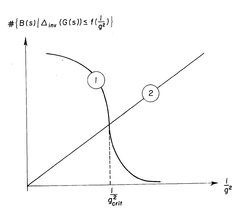
So the gauge ball $B(s^{\mu})$ is useful only if the associated group of transformations $G(s^{\mu})$ satisfy the criterion (45) above. The weaker the coupling (i.e., the larger the value of $\frac{1}{g^{2}}$) the smaller the allowed deviation from perfect symmetry ($\Delta_{dev}$) and the less likely it will be that a gauge ball is useful in the sense that (45) is satisfied. The density of such useful gauge balls decreases as the coupling for the $\phi_{h}(i)$ variables decreases; concurrently, the fundamental space-time points $i$ and associated field variables $\phi(i)$ lying within the gauge balls “rejected” according to the criterion (45) are no longer available for use in setting up a macroscopic $gA^{\mu}$ field. But it is necessary that such $gA^{\mu}$ can be set up if there are to be contributions to $\frac{1}{g^{2}}$ in the continuum limit.

Let us denote the number of gauge balls to which are associated sufficiently accurate symmetry $G(s^{\mu})$ groups (i.e., useful gauge balls) as

$$\#\{B(s^{\mu})|\Delta_{inv}(G(s^{\mu}))\leq f(\frac{1}{g^{2}})\}.$$ (46)

There are two competing relationships between $\frac{1}{g^{2}}$ and $\#\{B(s^{\mu})|\Delta_{inv}(G(s^{\mu}))\leq f(\frac{1}{g^{2}})\}$ (see Figure 6) that can be stated as follows:

1. the larger the number of “useful” gauge balls $\#\{B(s^{\mu})|\Delta_{inv}(G(s^{\mu}))\leq f(\frac{1}{g^{2}})\}$, the larger the number of microstate degrees of freedom $\phi$ that are connected to the macroscopic field $gA^{\mu}$ and hence the larger is $\frac{1}{g^{2}}$.

2. The weaker the coupling the more readily will there be long distance correlations in the field $H(s^{\mu})$ with the danger of Higgsing as a consequence; avoiding such correlations necessitates a smaller allowed deviation (45) from perfect symmetry for the groups $G(s^{\mu})$ associated with gauge balls $B(s^{\mu})$ and consequently a reduction in the number of “active” gauge balls $\#\{B(s^{\mu})|\Delta_{inv}(G(s^{\mu}))\leq f(\frac{1}{g^{2}})\}$.

Figure 6: There are two competing relationships between $\#\{B(s^{\mu})|\Delta_{inv}(G(s^{\mu}))\leq f(\frac{1}{g^{2}})\}$ and $\frac{1}{g^{2}}$ shown as curves 1 and 2. Curve 1 suggests the manner in which more and more gauge balls fail to satisfy (45) as $\frac{1}{g^{2}}$ increases. The suddenness with which curve 1 is depicted as dropping off with increasing $\frac{1}{g^{2}}$ is intended to suggest that $\#\{B(s^{\mu})|\Delta_{inv}(G(s^{\mu}))\leq f(\frac{1}{g^{2}})\}$ varies rapidly at the confinement to Coulomb phase transition. Curve 2 shows that $\frac{1}{g^{2}}$ increases with the number of useful gauge balls. Because of the rapid variation of curve 1 near $\frac{1}{g^{2}_{crit}}$, the intersection of the two curves can be expected to be at least very close to critical coupling values. Applying this argumentation to each possible partially confining phase, the analogue of the intersection of the two curves becomes the multiple point where all possible combinations of degrees of freedom can coexist in confinement and in configurations with long range correlations

The point to be made is that the field theory glass model for fundamental scale physics is a Random Dynamics scenario that, apart from yielding exact LEP gauge symmetry by the FNNS mechanism if there is an approximate symmetry at the fundamental scale, suggests that the inequality (2) is obeyed in Nature as an equality.

Point 1. above implies that having a value of $\frac{1}{g^{2}}$ that at the Planck scale is large enough to avoid confinement (i.e., the fulfilment of the inequality (2)) is really a question of having sufficiently many gauge balls that can be connected to a macroscopic $gA^{\mu}$ field. That the inequality (2) must be realised as an equality is suggested by point 2) above inasmuch as weaker than necessary couplings increase the risk of correlations over distances large enough to lead to Higgsing.

The two relations between $\frac{1}{g^{2}}$ and $\#\{B(s^{\mu})|\Delta_{inv}(G(s^{\mu}))\leq f(\frac{1}{g^{2}})\}$ (points 1. and 2. above) are depicted schematically in Figure (6). The suggestion that the inequality (2) is realised as a equality - if understood as applying to all possible partially confining phases - is tantamount to suggesting the validity of the principle of multiple point criticality.

2.5 Breakdown of the AGUT $SMG^{3}$ by confusion

As an inequality, (2) expresses the important requirement that Yang-Mills degrees of freedom at the Planck scale that give rise to the observed Yang-Mills fields of the Standard Model cannot, already at the Planck scale, have developed a strong coupling/high temperature/confinement-like physics. We make the important assumption that only Yang-Mills degrees of freedom that are Coulomb-like in behaviour at the fundamental scale have a chance of surviving down to experimentally accessible energies. This is what is insured by the inequality (2). In a simple lattice gauge theory with a gauge invariant action $S_{g.i.}$ given by $S_{g.i.}=\beta\sum_{\Box}ReU(\Box)$, confinement is avoided by having a large enough $\beta$.

However, a direction in the configuration space of a field theory glass along which there is only approximate gauge symmetry has accordingly at least small gauge breaking action contributions $S_{g.b.}$ to the quenched random action. We call this latter the fundamental action $S_{fund}$. Let us take as a prototype for $S_{g.b.}$ a term $S_{g.b.}=\kappa\sum_{\mbox{\begin{picture}(4.15,10.0)\put(0.0,3.0){\circle*{2.0}} \put(0.0,2.75){\line(1,0){7.0}} \put(7.3,3.0){\circle*{2.0}}\mbox{ } \end{picture} }}U(\mbox{\begin{picture}(4.15,10.0)\put(0.0,3.0){\circle*{2.0}} \put(0.0,2.75){\line(1,0){7.0}} \put(7.3,3.0){\circle*{2.0}}\mbox{ } \end{picture} })$ that explicitly breaks gauge symmetry.

The random dynamics philosophy for fundamental physics has played a decisive role in motivating the theoretical picture we have for the origin of the SMG via the $SMG^{N_{gen}}$ gauge group.

A possible theoretical motivation for the AGUT gauge group $SMG^{3}$ and its subsequent breakdown to the diagonal subgroup could start with a scenario from “random dynamics”[29, 26]: at an energy a little above the Planck scale, one has a multitude of gauge symmetries resulting from the FNNS exactification[28] of chance occurrences of approximate gauge symmetries. This collection of symmetries can be expected to be dominated by low-dimensional groups as such symmetries are most likely to occur by chance. We envision that the symmetry embodied by this collection of groups is broken down by a succession of steps the last of which, before the Weinberg-Salam breakdown, is the breakdown of the AGUT group $SMG^{3}$ to its diagonal subgroup. This succession of symmetry breakdowns is pictured as occurring for decreasing energies within a range of a few orders of magnitude at the Planck scale.

The succession of breakdowns envisioned coincides with gauge groups that are more and more depleted of group automorphisms. We (and others) have proposed a breakdown mechanism[20, 21, 22] called “confusion” that is active when gauge groups possess automorphisms.

We speculate that confusion breaking - that can be called into play by different types of automorphisms - can successively break very general groups with many Cartesian product factors down to a collection of groups with especially few automorphisms as is characteristic of the SMG itself. It is noteworthy that the SMG has been shown in a certain sense [30, 31] to be the group of rank 4 (and dimension less than 19) that is maximally deficient in automorphisms. We propose the group $SMG^{3}$ as the last intermediate step on the way to the SMG.

We now briefly explain how the confusion breakdown mechanism functions for gauge groups with outer automorphisms. First it is argued that, in the spirit of assuming a fundamental physics that can be taken as random, one is forced to allow for the possibility of having quenched random “confusion surfaces” in space-time. The defining property of these surfaces is that (e.g. gauge) fields obey modified continuity conditions at such surfaces; for example, the permutation of a gauge field with an automorphic image of the field can occur. A non-simply connected space-time topology is essential for the presence of nontrivial confusion surfaces; a discrete space-time structure such as a lattice is inherently non-simply connected because of the “holes” in the structure.

The essential feature of the “confusion” breakdown mechanism is that, in the presence of “confusion surfaces”, the distinct identities of a field and its automorphic image can be maintained locally but not globally. To see how this ambiguity arises, imagine taking a journey along a closed path on the lattice that crosses a confusion surface at which the labels of a gauge group element and its automorphic image are permuted. Even if one could, at the onset of the journey, unambiguously assign say the names “$Peter$” and “$Paul$” to two gauge fields related by an automorphism, our careful accounting of the field identities as we travel around the loop would not, upon arriving back at the starting point, necessarily be in agreement with the names assigned when we departed on our journey. So an attempt to make independent global gauge transformations of $Peter$ and $Paul$ (sub)groups would not succeed. Therefore, for the action at confusion surfaces, there is not invariance under global gauge transformations of the whole gauge group but only under transformations of the subgroup left invariant by the automorphism.

The ambiguity under the automorphism caused by confusion (surfaces) is removed by the breakdown of the gauge group to the maximal subgroup which is left invariant under the automorphism. The diagonal subgroup of the Cartesian product of isomorphic groups is the maximal invariant subgroup of the permutation automorphism(s); i.e., because the diagonal subgroup is the subgroup left invariant by the automorphism, it has the symmetry under gauge transformations generated by constant gauge functions (corresponding to the global part of a local gauge transformation) that survives after the ambiguity caused by the automorphism is removed by breakdown to the diagonal subgroup.

For the purpose of illustrating a possible origin of the “anti-unified” gauge group and its subsequent breakdown to the standard model group, we describe two important examples of group automorphisms - examples 1 and 2 below - that call the confusion mechanism into play:

Example 1.

Many groups have a charge conjugation-like automorphism corresponding in the $SU(N)$ case to complex conjugation of the matrices element by element. While for $SU(2)$ this is an inner automorphism, it is for higher $SU(N)$ groups an outer automorphism. According to the speculated confusion mechanism, such a group should break down to the subgroup consisting of only the real matrices which is the largest subgroup that is invariant under the automorphism. If the group is provided with C-breaking chiral fermions, the automorphism can be broken in this way thereby thwarting the “attack” from the confusion mechanism.

Example 2.

There can be automorphisms under the permutation of identical group factors in a Cartesian product group: we argue that the symmetry reduction (at the Planck scale) from $(SMG)^{N_{gen.}}$ to $SMG=S(U(2)\times U(3))$ is triggered by the symmetry under the automorphism that permutes the $N_{gen}$ SMG factors in $(SMG)^{N_{gen.}}$.

Elaborating briefly on example 1 above, we point out that with the exception of the semi-simple groups such as $SU(2)$, $SO(3)$ , the odd $N$ spin or $SO(N)$-groups and the symplectic groups, all groups have outer automorphisms of the complex conjugation- or charge conjugation-like type. Following a series of confusion breakdowns activated by charge conjugation-like automorphisms, we expect that the (intermediate) surviving gauge symmetry (i.e., that of $(SMG)^{N_{gen.}}$) must have matter fields that break charge conjugation-like symmetries. In other words, the presence of such matter fields serves to protect the surviving symmetry from further breakdown by eliminating the possibility for further confusion of the surviving group with its automorphic image under charge conjugation.

In particular, we expect that a necessary condition for the survival of gauge groups like $U(1)$ and $SU(3)$ is the presence of some matter fields not invariant under charge conjugation. Protection against this sort of breakdown can be provided by chiral fields that break the charge conjugation symmetry of the gauge fields. In the case of the Standard Model, left- and right-handed fermions always appear in different representations so that confusion breakdown by way of a charge conjugation automorphism is not possible. In fact, the number of particles in a single generation in combination with the rather intricate way these are represented in the Standard Model can be shown to be the simplest possible manner in which gauge anomalies can be avoided[32, 33, 34, 35].

As mentioned in example 2 above, it is assumed that the confusion breakdown of the intermediate gauge group $SMG^{3}$ to the standard model group SMG (at the Planck scale) is activated by the automorphism that permutes the $N_{gen}$ isomorphic Cartesian product factors in $(SMG)^{N_{gen.}}$. The elimination of the ambiguities that can arise in trying to keep track of the identities of a group element and its automorphic image under such permutations coincides with the breakdown to the standard model group $SMG=S(U(2)\times U(3))$ which, being the diagonal subgroup of $(SMG)^{N_{gen.}}$, is invariant under the automorphism that permutes the SMG group factors in $(SMG)^{N_{gen.}}$. In order for this final confusion breakdown to work effectively, the Cartesian product factors of $(SMG)^{N_{gen.}}$ must presumably be truly isomorphic - i.e., the matter field content of each factor must essentially have the same structure. This combined with the fact that one usual fermion generation is known to provide the least complicated arrangement of particles that avoids gauge anomalies would strongly suggest that the $N_{gen}$ factors of $(SMG)^{N_{gen.}}$ are simply dull repetitions of the standard model group each having a comparable matter field content but with the possibility of having different gauge quantum numbers as a distinguishing feature of the different families. Each of the $N_{gen}$ factors is the “ancestor” to one of the $N_{gen}$ generations of the diagonal subgroup identified with the usual Standard Model Group.

It should be emphasised that all the confusion breakdowns - those utilising a series of charge conjugation automorphisms leading to $(SMG)^{N_{gen.}}$ as well as the final confusion breakdown of the $SMG^{3}$ to the diagonal subgroup that is caused by the permutation automorphism - are assumed to take place within a rather narrow range of energies at the Planck scale.

Before leaving the confusion breakdown mechanism, we should point out that any mechanism that breaks the $SMG^{3}$ down to the diagonal subgroup would suffice for our model. A Higgs field mechanism could for example provide an alternative to the confusion mechanism of breakdown.

2.6 A string-regulated model using a Kaluza-Klein space-time

In this model, the Random Dynamics-inspired input is that the (quenched random) values of gauge couplings are given at the fundamental scale independent of low energy physics. This assumption can be implemented by insisting that, from the point of view of low energy physics, the value of gauge couplings at the fundamental scale must appear to be random. In the context of this model which will be briefly described now, it is argued that there is a range of fundamental scale coupling values that must be avoided if the suspicion of fine-tuning is not to be aroused. The weakest coupling in this range provides an upper limit on how strong a coupling should be observed experimentally.

Using a regularised Kaluza-Klein space-time at the fundamental scale with Yang-Mills fields in $D-4$ compactified dimensions, we examine the $\beta$-function for a dimensionless expression $\beta(1/a)=(2/g^{2})a^{D-4}$ for the coupling constants $g$ in $D$-dimensions. Here $a$ is the lattice constant and defines the renormalization point $\mu=1/a$. The “running” $\beta(\mu)$ is defined so as to describe observed continuum physics as a lattice with lattice constant $a=1/\mu$. The $\beta$-function for this $\beta(1/\mu)$ is shown to have an ultraviolet stable fixed point $\beta_{crit}$. The argument is that in order to avoid the suspicion that the values at the fundamental scale are fine-tuned to experimentally observed values (recall that couplings are assumed to be given at the fundamental scale independent of low energy physics), a small range of fundamental scale ($\approx$ Planck scale) coupling values centred at $\beta_{crit}$ must be avoided. Due to a scale dependent effective dimensionality $D$, this “forbidden” interval of values expands due to renormalization group effects into a large range of values in going towards the infrared that should not be observed at low (i.e., experimentally accessible) energies (see Figure 7. It is the larger $\beta$ boundary of the “forbidden” interval (at low energies) that provides an upper bound on “allowed” values for experimental couplings inasmuch as this boundary corresponds to being on the “Coulomb-like” side of $\beta_{crit}$ at the fundamental scale. The small $\beta$ boundary of the “forbidden” interval at low energies would correspond to a fundamental scale $\beta$ for which there was confinement already at the fundamental scale and accordingly would not lead to physics observable at low energies.

Figure 7: In the string regulated model using a Kaluza-Klein space-time with $D-4$ compactified dimensions at the fundamental scale, the idea is that in order not to arouse the suspicion of fine-tuning, a small interval centred at $\beta_{crit}$ at the fundamental scale must be avoided. This small “forbidden” interval $\epsilon$ expands due to renormalization group effects into a whole range of “forbidden” values of $\beta_{crit}$ that should not be observed in going to low energies. It is the upper limit of this range that provides an upper bound on allowed experimental couplings.

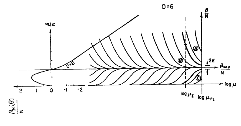
In this model, the scale dependence of the space-time dimensionality $D$ has several consequences. At the fundamental scale, the Kaluza-Klein space $\mbox{\bf{R}}^{4}\times K$ is of dimension $D>4$ but in going to lower energies, one at some point encounters the energy corresponding to the linear dimension $\rho$ of the compactification space $K$. At energies corresponding to distances longer than $\rho$, the dimensionality of space-time is reduced to $D=4$ and renormalization group effects are just the normal quantum mechanical ones. At the energy $1/\mu\approx\rho$ coinciding with the transition $D>4$ $\longrightarrow$ $D=4$, it is argued that couplings are weakened by a factor roughly equal to the number of fundamental string regulation volumes $reg.\;vol.$ that can be accommodated in the volume $vol(K)$ of the compactification space. Subsequently it is proposed that this factor cannot be less than the number of generations $N_{gen}$ by invoking an argument reminiscent of that sometimes encountered in string model “$T.O.E.$” the essence of which is that the quark and lepton generations correspond to various zero modes of a Weyl operator in the compactifying space.

Using string physics as a way of achieving a regularization of the Yang-Mills fields in the limit of zero slope is an alternative to a fundamental scale lattice as a way of implementing what we regard as the necessity of an ontological fundamental scale regularization in order that field theories be consistent. In a string theory, the compactification space $K$ is a continuum and what is needed, roughly speaking, is an argument for $vol(K)$ being large enough to accommodate a string from each generation without an overlapping of the domains of the different strings. A plausible line of reasoning would be that if the compactifying space $K$ becomes too small, the fields in $K$ corresponding to the zero modes could become so compressed and thereby so strong that the fluctuations giving rise to the extension of a string (corresponding for example to a gauge particle) become limited because the maximal string extension is constrained to be of the order of a typical length related to the field. For instance, it is quite possible that a string in a very curled-up Riemannian space with many niches and corridors will be constrained to be inside one (or several) of these niches even if this means that the string cannot have the usual $\sqrt{\alpha^{\prime}}$ extension.

As an example, we can think of a string as a rigid rotor on an $S_{2}$-sphere. If the sphere has a very small radius, even a string of small angular momentum (e.g. $l=1$) about a pole of the sphere can readily attain maximal extension - namely that corresponding to the ends of the string rotating in the equatorial plane. So in this case, the length of the string state (leading to a gauge particle) can be no more than $\pi r$ where $r$ is the radius of the $S_{2}$-sphere. This means that it is the scale of the curvature of the Riemannian space-time rather than the $\sqrt{\alpha^{\prime}}$ string extension that determines the string size in a very strongly curved space-time. In summary, the conclusion we want to make is that when a compactifying space of given topology (Euler number) is diminished in linear dimension, at some stage of this squeezing process, the property dictating the effective string regularization switches from being a characteristic of the string to being a characteristic of the curvature of the compactifying space. This in turn has the effect of “squeezing down” the otherwise string-determined regularization scale.

A variation on this scenario is the suggestion[36] that a string cannot be affected by the components in the background (e.g. gravitational) field having frequencies above the $\frac{1}{\sqrt{\alpha^{\prime}}}$ scale. Effectively this means that such components do not exist in which case it would be impossible to have the compactifying space-time of extent less than that necessary in order to have a curvature that is of the order $\alpha^{\prime}$. This would in turn mean that $\frac{vol(K)}{reg.\;vol.}$ would be at least of the same order of magnitude as the Euler number of $K$.

Arguments of the type just presented aid in justifying the assertion that, at least to order of magnitude validity, the effective number of regularization volumes in $K$ (namely $\frac{vol(K)}{reg.\;vol.}$) is larger than the number of zero modes $N_{gen}$. This form of argumentation together with the requirement that suspicions of fine-tuning be avoided leads to the inequality (2) in the slightly modified form

$$\beta_{experimental}(\mu_{Planck})\geq\frac{vol(K)}{{\cal N}_{0}}\geq N_{gen}\beta_{crit}.$$ (47)

Here $\beta_{experimental}(\mu_{Planck})$ denotes the experimental values of the inverse squared couplings (one for each of the SMG subgroups $SU(3)$, $SU(2)$, and $U(1)$ that have been extrapolated to the Planck scale using the assumption of a “desert” in the renormalization group extrapolation. The lower bound $N_{gen}\beta_{crit}$ of the inequality (47) depends obviously on $N_{gen}$ as well as $\beta_{crit}$. The latter tends to be larger the larger the group. This is corroborated for $SU(N)$ groups by the approximate relationship

$$\frac{\beta_{crit,\;M.F.A.}}{N}\approx 0.8$$ (48)

known from studies using the Mean Field Approximation ($MFA$). It is shown that for $N_{gen}=3$ and for a $SU(N)$ group with $N=3$, the lower limit $N_{gen}\beta_{crit}$ is pushed so high up in value that the experimentally observed inverse squared couplings are only just barely large enough to escape the “forbidden gap”. In fact, a gauge group no larger than $SU(5)$ would be on the verge of predicting less than three generations of fermions in the “forbidden gap” is to be avoided. This allows several tentative conclusions:

1. There is not “room” for many more than the three experimentally known generations of quarks and leptons.

2. Grand unification cannot be accommodated in the 4-dimensional scale region as this would increase $\beta_{crit}$ prohibitively; in fact, grand unification could only be tolerated at a scale close to the Planck scale. This implies a large desert. Already for $SU(2)$ and $SU(3)$ the inequality (47) is close to being saturated insofar as $N_{gen}$ is experimentally established as not being less than three.

3. A “blooming” of the desert in excess of that already “known” to couple to the SMG Yang-Mills fields is not allowed inasmuch as additional scalars or fermions at low energies would make unwelcome contributions to the 4-dimensional Callan-Symanzik $\beta$-function.

4. The compactifying space $K$ should be no larger “than necessary”; i.e.,., $vol(K)$ should not exceed the number of generations times the regulation volume of a fundamental string region.

5. At the string or fundamental scale, the couplings are expected only to be just enough larger so as not to arouse the suspicion of fine-tuning.

3 The principle of multiple point criticality

A central theme of this work can be stated as a proposed fundamental principle - the principle of multiple point criticality. This principle has evolved from being a specific assertion about the values assumed by the gauge fine-structure constants in the context of a Yang-Mills lattice gauge theory to a general statement about Nature that essentially aspires to be a solution to all the fine-tuning paradoxes in fundamental physics. In the specific context in which this principle originated, it can be stated as follows:

At the fundamental scale (taken to be the Planck scale), the actual running gauge coupling constants correspond to the multiple point critical values in the phase diagram of a lattice gauge theory.

In this context, the multiple point is a point in the phase diagram of the lattice gauge theory at which all - or at least many - “phases” convene. This point corresponds to critical values for the parameters used to describe the form of the action. In the rather crude mean field approximation considered here, there is one “phase” for each combination $(K,H)$ where $K$ is a subgroup of the gauge group $G$ and $H$ is an invariant subgroup of $K$; i.e., there is a “phase” for each combination $(K\subseteq G,H\lhd K)$ where $H$ can also be a discrete invariant subgroup.

If one adopts the viewpoint that the actual existence of a fundamental regulator is a prerequisite for the consistency of any field theory at sufficiently short distances, then one must accept phases distinguishable at the scale of the regulator as also being real and physically existing. In this context, the MPCP would assert that there is an affinity for parameters corresponding to the junction of a maximum number of “regulator-scale” distinguishable phases regardless of how the ontological regulator of field theories at the fundamental scale is implemented. We have considered the MPCP in the context of a lattice regulator; however, assuming that such a fundamental regulator can be formulated or implemented in ways alternative to a lattice (e.g., as strings), a credible MPCP would need to give the same values of, for example, fine-structure constants upon seeking out the junction of a maximum number of phases distinguishable at the scale of the alternative regulator.

3.1 Multiple Point Criticality: a prototype for fine-tuning

3.1.1 What are fine-tuning problems?

One has a fine-tuning problem when the experimental values of physical constants are found to have very special values relative to an a priori expectation. An explanation of why constants of Nature have seemingly non-generic values cries out for a theoretical explanation. Why for instance is the cosmological constant so exceedingly small in terms of Planck scale units, which one would naturally suspect were the fundamental units in Nature? Why is the Higgs expectation value, which determines the weak interaction scale, so small compared to the Planck mass or, if one believes in Grand Unification, to the unification scale? Addressing the fine-tuning problems offers the hope of being able to use hints coming directly from Nature - rather than from pure speculation - to learn about what the physics should be like at much shorter distances than those presently accessible and known.

The values assumed by the fine-structure constants of the Standard Model also constitute a fine-tuning problem in that these rather remarkably take the values at “the” multiple point. In the formulation that we have used so far, the multiple point is the point in the phase diagram of a lattice gauge theory (having a sufficiently general plaquette action) at which all - or at least many - phases convene. Actually the experimental values of the fine-structure constants only coincide with the multiple point values if we make the assumption of an AGUT gauge group[3, 37, 38, 39, 7, 20, 21, 22] with the gauge group $SMG^{3}$ (which is the 3-fold Cartesian product of the “usual” Standard Model Group (SMG): $SMG^{3}\stackrel{{\scriptstyle def}}{{=}}SMG\times SMG\times SMG$). The “usual” Standard Model Group $SMG=S(U(2)\times U(3))$ arises as the group surviving the Planck scale breakdown of $SMG^{3}$ to its diagonal subgroup. With the anti-grand unified gauge group $SMG^{3}$, each generation acquires its own 12 gauge fields just as in the Standard Model). Hence, if the assumption of the gauge group $SMG^{3}$ etc. is accepted as the immediate (Planck scale) predecessor to the $SMG$, it is indeed a fine-tuning problem that is addressed in explaining why the fine-structure constants should take just the multiple point values, on a par with explaining the smallness of, for example, the cosmological constant.

We propose that all the fine-tuning problems, including the fine-structure constant one, are unified (or at least reformulated) if it is assumed that Nature in general has an affinity for the multiple point, where a lot of phases meet for a single combination of the “intensive parameters”. The latter are really just parameters of the action. Included among such parameters - generalised “coupling constants” - are lattice artifact parameters. This is because we take the lattice as really existing, in the sense that a lattice is one of many ways of implementing what we assume to be the actual existence of a fundamental regularization at roughly the Planck scale. This assumption is inspired by the fact that the consistency of any field theory seems to require a cut-off.

3.1.2 How does multiple point criticality solve fine-tuning problems?

So our basic explanation for the fine-tuning problems is that, for some reason, the coupling constants etc. in Nature take values that correspond to the multiple point where “all” (or as many as possible) phases convene.

An analogous phenomenon is known from other fields of physics: e.g., a mixture of ice and water (and vapour) chooses its temperature and pressure to be that of the melting point (the triple point). By mixtures of well chosen but not fine-tuned amounts of various different molecules, it would be possible to realise a multiple point with more than just three phases that convene. Here it is the enforced coexistence (insured by choosing combinations of extensive quantities like mole number, energy and volume such that the universe is not realizable as a single phase) of the phases that consequently enforces the multiple point values for the chemical potentials, temperature and pressure so that there is a balance w.r.t. exchange of molecules between the phases.

It is very tempting to speculate that an analogous scenario, in which there are (e.g., primordially) fixed but not fine-tuned amounts of perhaps a great many extensive quantities (analogous to number of molecules, energy and volume in the above example), can provide an explanation for all fine-tuned quantities in Nature. We shall see in the sequel that having fixed amounts of extensive quantities in, say, the universe implies a mild form of non-locality (or vice versa) that, in turn, implies multiple point criticality and thereby universally fixed physical constants.

3.2 Fine-tuning demands non-locality

In this section it is argued that at least the cosmological constant fine-tuning problem really calls for the breakdown of the principle of locality in the mild sense referred to above. Any fine-tuning problem concerning coupling constants - among which we may also include the cosmological constant - calls for some way by which these coupling constants are rendered “dynamical”, in the sense that their values are not simply fixed a priori but can in some way take on values that must (for the sake of translational invariance) be maintained at a constant value. That a physical constant (e.g., coupling constant) can depend on something (i.e., in spite of being constant as a function of space-time, is not simply fixed a priori) is the most important content of the baby-universe[40, 41, 42, 43, 44] theory. The latter theory indeed aspires with some success to solve the cosmological constant problem. The baby-universe theory also makes use of an effective breakdown of the principle of locality and renders the coupling constants dynamical. Hereby this theory has the right ingredients needed if the goal of explaining why the cosmological constant is small is to be achieved .

The problem in local theories - i.e., healthy theories inasmuch as locality is seemingly well confirmed - is that, if the coupling constants and in particular the (bare) cosmological constant are “dynamical”, the strict validity of a principle of locality in the theory would imply that the bare dynamical cosmological constant could only depend on the situation at the space time point in question and, indirectly, also on previous times but certainly not on the future! However, a bare cosmological constant that is constant in space-time should already in the first moment after the Big Bang have had its value fine-tuned once and for all - up to, say, 120 decimal places - to the value which makes the dressed (renormalised) cosmological constant so exceedingly small (as only can be seen in a background so depleted of matter as is the case today). That means that the bare constant had to “know” about the details of a vacuum that did not exist at the time when the bare cosmological constant was already tuned in to the vacuum that would eventually evolve! Such a tuning of the bare cosmological constant seems to need some form of pre-cognition! But this is precisely what is achieved by breaking the principle of locality. So we are forced to accept that at least a strict principle of locality is not allowed, if we are to explain the cosmological constant problem in a way commensurate with having dynamical (bare) couplings and the renormalization corrections of quantum field theory with a well-defined vacuum.

3.2.1 The possibility for having non-locality commensurate with phenomenology

In [7] it is argued that, even if the principle of locality were indeed broken at the fundamental level, it might be regained effectively by restricting the breakdown of locality to a form that does not violate the principle of general reparameterization invariance of general relativity.

A theory having non-localities extending only over fundamental scale distances may usually be considered local when viewed at distances long compared to the fundamental scale. So the form of non-locality that potentially could be in conflict with the phenomenologically obeyed principle of locality must involve distances much longer than the fundamental scale (the Planck scale say). We want to argue that even non-locality over extremely large distances is not in conflict with what we regard as the phenomenological validity of the principle of locality, if the (long distance) non-locality is restricted to being invariant under diffeomorphisms or reparameterization. This class of non-locality includes that of interest to us - namely nonlocal interactions surviving at distances much longer than the fundamental scale and that are the same between the fields at any pair of points in space-time independent of the distance between these points.

Figure 8: Exponential decay of interaction coefficients $c(x,y)$ as a result of quantum gravity fluctuations[7] (Figure from a lecture by H.B. Nielsen in his course “Q.C.D. etc.”).

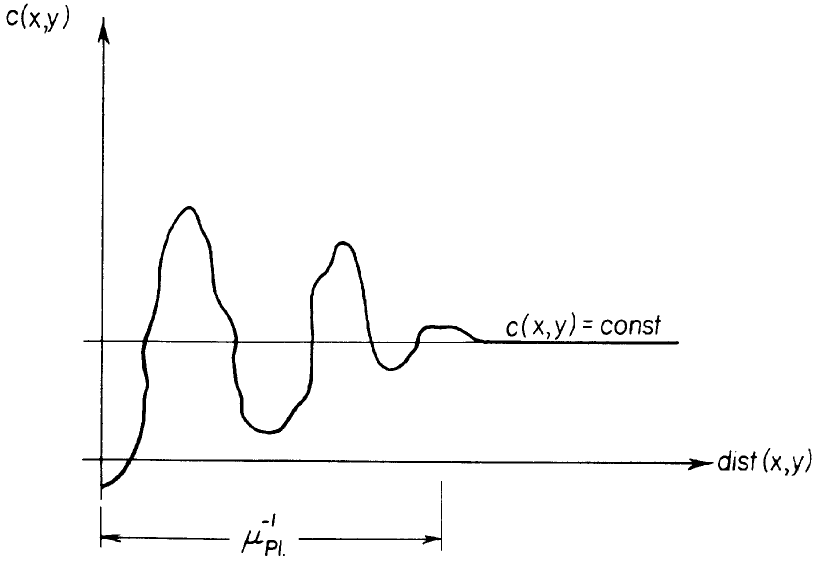
It can be argued[7] that quantum gravity fluctuations will at large distances $\int_{x}^{y}ds$ smooth out the effective interaction between a pair of fields $\phi(x)$ and $\phi(y)$ in such a way that interaction coefficients $c(x,y)$ decay exponentially as a function of distance to values independent of the distance $\int_{x}^{y}ds$: i.e., $c(x,y)=const.$ Here the $c(x,y)$ are defined by there being an action term

$$\int\int d^{4}xd^{4}y\sqrt{g(x)g(y)}c(x,y){\cal L}_{i}(x){\cal L}_{j}(y).$$ (49)

The expected exponential decay of $c(x,y)$ to the long distance constant value $const.$ has decay rates not differing by more than a few orders of magnitude from the fundamental scale. Hence, for the purposes of very long distances, (49) becomes

$$const.\cdot\int\int d^{4}xd^{4}y\sqrt{g(x)}\sqrt{g(y)}{\cal L}_{i}(x){\cal L}_{j}(y)\stackrel{{\scriptstyle def}}{{=}}const.\cdot I_{i}I_{j}$$

The interaction between a number of fields can similarly be taken into consideration, in such a way that the long distance physics takes the form of non-linear functions of integrals $I_{j}=\int d^{4}x\sqrt{g(x)}{\cal L}_{j}(x)$. Here the ${\cal L}_{i}(x)$’s denote expressions of the type that could be usual Lagrangian density terms. The reparameterization invariance of general relativity is in essence assumed in this argumentation.

Indeed a principle like reparameterization invariance is needed, in order to have a symmetry between all pairs of space-time points that implies the same interaction between all such pairs regardless of the distance separating them.

The important point is that an interaction that has the character of being the same between the fields located at any pair of points (regardless of separation) is really hardly perceivable as a nonlocal interaction. Rather we would tend to interpret such effects as being a part of the laws of Nature, since such effects are forever everywhere the same. Such an omnipresent effect is therefore effectively unobservable and we would not in practice see any deviation from locality.

Finally, having once renounced a strict principle of locality, it is natural to go a step further and enquire as to whether it might be possible for fields to depend on more than one space-time point (separated by large distances). We propose that such fields might cause a spontaneous breakdown of reparameterization invariance, so that distant points in space-time become related. Degrees of freedom at distant points, related by this breakdown, would be interpreted as several degrees of freedom at the same point. Such a field replication mechanism that comes from “explaining away” ontological non-locality would be welcome, as a possible explanation for the 3-fold replication seen in the three generations of quarks and leptons. This possibility is discussed more extensively in Section 3.2.4. That a 3-fold replication mechanism for fermions would, probably unavoidably, also provide a 3-fold replication of bosons is also a very welcome prediction in the context of the AGUT gauge group model that uses the gauge group $SMG^{3}$ (i.e., the 3-fold Cartesian product of the Standard Model Group). This gauge group, the Planck scale breakdown of which yields the normal SMG in our model, is an important ingredient in our predictions of gauge couplings using multiple point criticality.

3.2.2 Non-locality as the underlying explanation of the affinity of Nature for a multiple point

We shall now argue that the assumption of non-locality implies having the the principle of multiple point criticality. For the purpose of explaining why Nature seeks out the multiple point, we assume in accord with the argumentation of Section 3.2.1 that we have fields $\phi$ depending on a single space-time point that interact non-locally, in such a way that the long distance remnants of the nonlocal interactions between fields $\phi(x)$ and $\phi(y)$ are the same for all pairs of space-time points $x$ and $y$. As the reparameterization invariance of general relativity implies this symmetry between space-time points, we write our nonlocal action as a non-linear function of reparameterization invariant integrals of the form

$$I_{j}\stackrel{{\scriptstyle def}}{{=}}\int d^{4}x\sqrt{g(x)}{\cal L}_{j}(x)$$ (50)

where the ${\cal L}_{j}$ denote the usual sort of terms in a local Lagrangian density. An ${\cal L}_{j}$ could, for example, be a polynomial of degree $n$ in the (scalar) field $\phi(x)$: ${\cal L}_{j}=\phi^{n}(x)$ or the $k$th partial derivative of such a field: ${\cal L}_{j}=\partial^{k}\phi^{n}(x)$ (somehow made rotationally invariant).

We achieve non-locality by considering actions $S_{nl}(I_{1},I_{2},...,I_{N})$ that are non-linear functions of the integrals $I_{j}$. Note that nonlinearity is tantamount to non-locality, because nonlinearity in the quantities $I_{j}$ implies having integrals with more than one integration variable; e.g., an action term $\propto I_{i}I_{j}$ is indeed nonlocal because

$$I_{i}I_{j}=\int\int d^{4}xd^{4}y\sqrt{g(x)}\sqrt{g(y)}{\cal L}(x)_{i}{\cal L}(y)_{j}$$

contains contributions from fields at independent (and therefore in general different) space-time points $x$ and $y$. Note that had we taken a linear function of the integrals $I_{j}$: $S=\sum g_{j}I_{j}$, we would get an ordinary local action.

An important property of the reparameterization invariant integrals $I_{j}$ is that any function of such integrals - even a non-linear and thereby nonlocal one - is also reparameterization invariant. So we can say that we restrict the non-locality allowed in our model to the non-locality that comes about, due to having an action that is a non-linear function of a lot of integrals $I_{j}$ having integrands corresponding to the various Lagrangian densities ${\cal L}_{j}$ being used. Our speculation is that this form of non-locality (formulated with the $I_{i}$’s) is really the only form that can survive at long distances, when reparameterization invariance is insisted upon (see however Section 3.2.4 for a generalisation).

However, we now want to argue that this restricted form of non-locality would not be easily observable and could therefore really exist in Nature without ever having been observed as, for example, an “action at a distance” sort of non-locality. Rather we would say that the only traces of the restricted form of non-locality that we consider are (some) solutions of fine-tuning problems.

Formally we can think of having the functional integral of Nature with a nonlocal action $\hat{S}_{nl}$ that is a functional of the fields $\phi$ of the theory:

$$\int{\cal D}\phi e^{i\hat{S}_{nl}[\phi]}.$$ (51)

where

$$\hat{S}_{nl}[\phi]\stackrel{{\scriptstyle def}}{{=}}S_{nl}(I_{1}[\phi],I_{2}[\phi],\dots I_{N}[\phi])$$ (52)

and $\phi$ is used as a symbol for all the fields of the theory. As with any classical approximation for a field theory, it can be argued that this functional integral is dominated by field values in the neighbourhood of the field values $\phi_{0}$ for which the action is stationary:

$$\frac{\delta\hat{S}_{nl}}{\delta\phi}|_{\phi_{0}}=0.$$ (53)

Were the quantities $I_{i}$ effectively independent, we would deduce from Eq. (53) that

$$\frac{\partial S_{nl}(\{I_{i}\})}{\partial I_{j}}=0.$$ (54)

If there are some necessary relations between the $I_{i}$’s, because of their functional forms as functionals of the same fields $\phi$, the $I_{i}$’s may be constrained to take values in only some allowed region of the space spanned by the $\{I_{i}\}$ (see Figure 9 for an example). In the event that $S_{nl}$ has an extremum on the border of the allowed region, we should only require that the variation of $S_{nl}$ vanish along this border. In this event,

$$\frac{\partial S_{nl}(\{I_{i}\})}{\partial I_{j}}=\lambda a_{j}.$$ (55)

where the variation along the border obeys the restriction $\sum a_{j}dI_{j}=0$ and $\lambda$ is a Lagrange multiplier. If the border is of co-dimension greater than one, there will be a Lagrange multiplier for each co-dimension and a corresponding contribution in Eq. (55).

We illustrate the idea of how a nonlocal reparameterization invariant action can lead to fine-tuning by an example in which we ignore derivative terms in the action. Thus we consider only a nonlocal pure scalar field potential type action, in which the potential term is nonlocal at very long distances in such a way that the interaction is independent of the distance between space-time points. This is insured by taking a nonlocal potential $\hat{V}_{nl}[\phi]=V_{nl}(\{I_{j}[\phi]\})$ that is a (non-linear) function of the quantities $\{I_{j}\}$.

We now seek the minimum for a nonlocal potential $V_{nl}(\{I_{j}\})$ in a space spanned by quantities $I_{j}/V$ - i.e., the volume densities of the quantities $I_{j}$. For illustrative purposes we consider the simple situation in which there are just two quantities $I_{1}$ and $I_{2}$ where

$$I_{1}=\int d^{4}x\sqrt{g(x)}\phi(x)\stackrel{{\scriptstyle def}}{{=}}\int d^{4}x\sqrt{g(x)}v_{1}(\phi(x))$$ (56)

and

$$I_{2}=\int d^{4}x\sqrt{g(x)}(\phi^{4}(x)-5\phi^{2}(x)+\phi(x))\stackrel{{\scriptstyle def}}{{=}}\int d^{4}x\sqrt{g(x)}v_{2}(\phi(x))$$ (57)

where $v_{2}(\phi(x))$ is some polynomial that, for illustrative purposes, is taken as being 4$th$ order; e.g., $v_{2}(\phi(x))=\phi^{4}(x)-5\phi^{2}(x)+\phi(x)$.

One should bear in mind that the integrals $I_{1}$ and $I_{2}$ of field polynomials over space-time cannot take values that are completely independent of each other. If, for instance, the integral $I_{2}$ of $v_{2}(\phi(x))$ over space-time is required to be rather small, the value of $\phi$ cannot be too large over most of space-time. This in turn would limit the possible values of the integral over space-time of $\phi$ itself. Taking such relationships into account leads to an allowed region of values for the $\{I_{j}\}$. Including many polynomials in the fields $\phi$ can lead to allowed regions that can be somewhat complicated. We shall continue to restrict our example to the two quantities $I_{1}$ and $I_{2}$ defined above. Figure 9 depicts schematically the allowed region of $I_{1}$ and $I_{2}$ values, with values of $I_{1}/V=\langle\phi\rangle$ plotted along the abscissa and $I_{2}/V=\langle v_{2}(\phi)\rangle$ along the ordinate. The average $\langle\rangle$ denotes an average over space-time. The part of the boundary of the convex envelope of allowed values drawn as the heavy solid curve corresponds to having a constant $\phi(x)$ in space-time: $\phi(x)=I_{1}/V$.

Figure 9: The nonlocal potential $V_{nl}(I_{1},I_{2})$ can have its minimum at any point in the interior (e.g., point 3) or on the boundary (e.g., points 1 or 2) of the convex closure of allowed $(I_{1}/V,I_{2}/V)$ combinations (the cross-hatched area). The three inserts show the characteristic form of the effective local potential $V_{eff}$ at the three generic possibilities for the minima of $V_{nl}$. For minima of $V_{nl}$ at interior points, $V_{eff}$ is just flat (see insert at point 3). At minima of $V_{nl}$ on the heavy solid curve portion of the boundary, the characteristic feature of $V_{eff}$ is one absolute minimum (see insert at point 1) corresponding to $(I_{1}/V,I_{2}/V)$ combinations realisable in a universe with just one (dominant) value of $\phi(x)$ in the vacuum. At minima of $V_{nl}$ located at boundary points indicated by the heavy broken line, the characteristic feature of $V_{eff}$ is two equally deep minima (see insert at point 2), corresponding to $(I_{1}/V,I_{2}/V)$ combinations that can be realised as the vacuum of a universe having different dominant constant values of $\phi(x)$ in different space-time subregions.

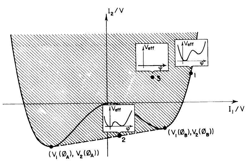
A priori, the nonlocal potential $V_{nl}(I_{1},I_{2})$ can have its minimum at any point in the interior (the cross-hatched region of Figure 9) or on the boundary of the allowed region (convex envelope). The heavy solid curve of Figure 9 corresponds to the $(I_{1}/V,I_{2}/V)$ combinations that can be realised in a universe having just one dominant value of (i.e., almost everywhere in space-time constant) $\phi(x)$ in the vacuum. Here the symbol $V$ denotes the volume of the universe. That is, $\phi(x)=\langle\phi\rangle$ for almost all of space(time). Allowed $(I_{1}/V,I_{2}/V)$ combinations, not lying on the heavy solid curve portion of the boundary of the convex envelope, cannot be realised in a universe having a single dominant (for all space-time) constant value of $\phi(x)$. However, such points can be realised by means of a positively weighted linear combination of points on the heavy solid curve. Such points would correspond to a universe the vacuum of which has different dominant constant values of $\phi(x)$ in different space-time subregions, where the extent of these subregions in space-time is proportional to the positive weights needed, in the combination of the several constant values of $\phi(x)$, to get a universe having the average values $\langle\phi\rangle=I_{1}/V$ and $\langle v_{2}(\phi)\rangle=I_{2}/V$.

In Figure 9, we also indicate with the points 1, 2 and 3 representatives for the three generic classes of points, in the convex envelope of allowed $(I_{1},I_{2})$ combinations, at which $V_{nl}(I_{1},I_{2})$ can have its minimum: point 3 represents the interior, point 1 represents the class of points on the heavy solid curve coinciding with the boundary of the convex envelope, and point 2 is a prototype for the remainder of the boundary of the convex envelope. It is reasonable to claim that all of these 3 prototypes represent generic possibilities - even though one might a priori think that a minimum on the border would require some degree of fine-tuning.

A moment’s reflection can perhaps convince the reader that a point such as 3 can be obtained as a suitably (positively) weighted combination of infinitely many points on the heavy solid curve in Figure 9. Points on this heavy solid line in Figure 9 (i.e., points of type 1) correspond to universes that can only be realised with fields that are almost everywhere equal to the average values of these fields (i.e., essentially the same constant value for $\phi(x)$ at almost all space-time points $x$): $\forall x,\;\phi(x)=\langle\phi\rangle$. Indeed a point such as 1 on the convex closure of the convex envelope of allowed $(I_{1}/V,I_{2}/V)$ combinations can only be obtained as a single-term “combination” of different constant values of $\phi(x)$ - namely the constant value of $\phi(x)$ at the point 1.

The final prototype point at which $V_{nl}(I_{1},I_{2})$ can have its minimum - the interesting case as it turns out - is point 2, located on the closure of the convex envelope that is not on the heavy solid curve. Such a point corresponds to a universe not realisable with a single constant (i.e., everywhere in space-time constant) value of $\phi(x)$.

At such a point, there are only two constant values of $\phi(x)$ (having one constant value at points in some space-time subregion and the other constant value at all other points in space-time) that together can participate in a weighted combination that can realise the prototype point 2. These are the constant values, $\phi=\phi_{A}$ and $\phi=\phi_{B}$, at the points on the convex closure at which the heavy broken line of universes, un-realisable with single constant values of $\phi(x)$, is tangent to the heavy solid curve (corresponding to all universes that are realisable with a single value of $\phi(x)=\langle\phi\rangle$):

$$\frac{I_{1}}{V}=\langle\phi_{point\;2}\rangle=w_{A}\phi_{A}+w_{B}\phi_{B}\;\;\;(w_{A}+w_{B}=1)$$ (58)

where $w_{A}$ is proportional to the extent of the space-time region having the constant value $\phi_{A}$ and $w_{B}$ to that of the space-time region having the constant value $\phi_{B}$.

We want to examine the effective local potential in the three cases, in which the nonlocal potential is located at the three types of points 1, 2 and 3.

The effective local potential $V_{eff}$ is defined as that function of $\phi$ for which the derivatives are equal to the corresponding (functional) derivatives of the nonlocal potential $V_{nl}$. We can think of $V_{eff}$ as the potential observed in a laboratory very small compared to the volume of the universe and arbitrarily placed at some space-time point. The derivative of $V_{eff}$ is the change in $V_{eff}$ observed in the laboratory, when the value of the field $\phi$ is changed only in the laboratory and kept constant at all other points of space. If $\phi$ is changed by a finite amount in the laboratory, the effective local potential can be integrated up: $V_{eff}(\phi_{A})-V_{eff}(\phi_{B})=\int^{\phi_{B}}_{\phi_{A}}V_{eff}^{\prime}(\phi)d\phi$.

Formally we make the definition

$$\frac{\partial V_{eff}(\phi(x))}{\partial\phi(x)}\stackrel{{\scriptstyle def}}{{=}}\frac{\delta V_{nl}(\{I_{j}[\phi]\})}{\delta\phi(x)}\left|{}_{near\;\;min.}\right.=\sum_{i}\left(\frac{\partial V_{nl}(\{I_{j}\})}{\partial I_{i}}\frac{\delta I_{i}[\phi]}{\delta\phi(x)}\right)\left|{}_{near\;\;min.}\right.$$ (59)

$$=\sum_{i}\frac{\partial V_{nl}(\{I_{j}\})}{\partial I_{i}}\left|{}_{near\;\;min.}\right.v_{i}^{\prime}(\phi(x))$$

This definition implicitly assumes that, to a very good approximation, $V_{nl}$ takes on its lowest possible value. But this does not preclude small regions of space-time from having $\phi$ values that deviate, by essentially any desired amount, from the average value(s) in the vacuum or vacua. The subscript “near min” in this formula denotes the approximate ground state of the whole universe, up to deviations of $\phi(x)$ from its vacuum value (or vacuum values for a multi-phase vacuum) in relatively small regions.

As a solution to Eq. (59) we have

$$V_{eff}(\phi)=\sum_{i}\frac{\partial V_{nl}(\{I_{j}\})}{\partial I_{i}}v_{i}(\phi)$$ (60)

where the $v_{i}(\phi)$ are the (field polynomial) integrands of the “extensive” (reparameterization invariant) quantities $I_{j}=\int d^{4}x\sqrt{g(x)}v_{j}(\phi(x))$. We can identify the $\frac{\partial V_{nl}(\{I_{j}\})}{\partial I_{i}}$ as intensive quantities conjugate to the $I_{i}$.

That Eq. (60) solves Eq. (59) is easily seen by differentiating Eq. (60) and using that the right hand side of Eq. (59) is $\sum_{j}\frac{\partial V_{nl}}{\partial I_{j}}\frac{\delta I_{j}[\phi]}{\delta\phi}=\sum_{j}\frac{\partial V_{nl}}{\partial I_{j}}v_{j}^{\prime}(\phi(x))$. The seeming $x$-dependence of this right-hand side of (59) for prescribed values of $\phi(x)$ is effectively absent due, at the end, to the reparameterization invariance hidden in the form of the $I_{j}$’s.

We now proceed with a study of the effective potential $V_{eff}$ for the field configurations $\phi$ near the minimum of $V_{nl}$, when this minimum is near one of the three types of points 1, 2 and 3.

At an interior point of type 3, the absolute minimum of $V_{nl}$ is also a local minimum and $\frac{\partial V_{nl}(\{I_{j}\})}{\partial I_{i}}=0$ for all $i$. Accordingly,

$$V_{eff}=\sum_{i}\frac{\partial V_{nl}}{\partial I_{i}}\left|{}_{near\;\;min.\;\;at\;\;``3"}v_{i}(\phi)=0\right.$$ (61)

So when $V_{nl}$ has its minimum in the interior, the effective potential $V_{eff}$ is flat. Recall that an interior point such as 3 can be obtained as a suitably (positively) weighted combination of infinitely many points on the boundary of the allowed region. This is related to the fact that $V_{eff}$ has infinitely many minima (because it is flat) at an interior point at which $V_{nl}$ has its minimum.

If $V_{nl}$ has its minimum at a point of the type 1 or 2 (i.e., on the border of the convex envelope), we have in general that

$$V_{eff}=\sum_{i}\frac{\partial V_{nl}}{\partial I_{i}}\left|{}_{near\;\;min.\;\;at\;\;``1"\;\;or\;\;``2"}\;v_{i}(\phi)\neq 0\right.$$ (62)

because in general $\frac{\partial V_{nl}(\{I_{j}\})}{\partial I_{i}}\neq 0$ at an absolute minimum of $V_{nl}$ located on the boundary of the convex envelope.

For the minimum of $V_{nl}$ located at a point of the type 1, there is only one value of $\phi(x)$ realised in the vacuum (i.e., in extended regions of space-time) - namely the value $\langle\phi\rangle=I_{1}/V$ at which the minimum of $V_{nl}$ is located. Accordingly, $V_{eff}$ has a single deepest minimum - namely that at $\phi_{1}$ where the latter denotes the value of $I_{1}/V$ at the point 1 on the convex closure where $V_{nl}$ has its minimum.

That there is only one deepest minimum at a type 1 point is readily seen, by showing that the assumption of a second equally deep minimum at some other value $\phi_{C}$ would lead to a contradiction. First we make the observation that the gradient of $V_{nl}$, which cannot be zero for a generic point of type 1, is perpendicular to the tangent to the convex envelope at point 1. Secondly, note that the line connecting $\phi_{1}$ with $\phi_{C}$ determines a chord of the convex envelope that necessarily lies in the interior of the convex envelope. A displacement away from point 1, along such a chord, has therefore always a component along the gradient of $V_{nl}$. But moving along this chord, defined by the two equally deep minima in $V_{eff}$ at respectively $\phi_{1}$ and $\phi_{C}$, corresponds to replacing $\phi_{1}$ by $\phi_{C}$ (or vice versa) in a small space-time region at no cost in energy. This is inconsistent with the observation that a displacement along this chord necessarily has a component along the gradient of $V_{nl}$. We conclude that $V_{eff}$ cannot have two (or more) equally deep minima.

The most interesting case is that for which the minimum of $V_{nl}$ is located at a point of type 2 (with coordinates denoted as $(I_{1},I_{2})_{type\;2}$, see Figure 9) on the convex closure of the convex envelope of the allowed region. Such a universe cannot be realised with $(\phi(x),v_{2}(\phi(x)))=(I_{1}/V,I_{2}/V)_{type\;2}$. It can be shown that, in order to realise $(I_{1}/V,I_{2}/V)_{type\;2}$, only the two constant contributions $(\phi_{A},v_{2}(\phi_{A}))$ and $(\phi_{B},v_{2}(\phi_{B}))$ can participate in the (unique) weighted combination. A universe corresponding to the point $(I_{1}/V,I_{2}/V)_{type\;2}$ could be realised with the field

$$\phi(x)=\left\{\begin{array}[]{c}\phi_{A}\mbox{\footnotesize{ for $x$ $\in R_{A}$ }}\\ \phi_{B}\mbox{\footnotesize{ for $x$ $\in R_{B}$}}\end{array}\right..$$ (63)

where $R_{A}$ and $R_{B}$ are large regions of space-time.

It is interesting that two minima of $V_{eff}$ will be seen to have the same depth. This is tantamount to fine-tuning, in that the relation $V_{eff}(\phi_{A})=V_{eff}(\phi_{B})$ can be used to eliminate a bare parameter (for example, the bare Higgs mass $m_{H}$). Having two equally deep minima of $V_{eff}$, for $\phi_{A}$ and $\phi_{B}$, is characteristic of a vacuum with two coexisting phases. This is tantamount to being at the multiple point.

That we in fact have $V_{eff}(\phi_{A})=V_{eff}(\phi_{B})$, when the minimum of $V_{nl}$ is at a type 2 point, can be seen by considering the directional derivative of $V_{nl}$ along the line connecting the points $(\phi_{A},v_{2}(\phi_{A}))$ and $(\phi_{B},v_{2}(\phi_{B}))$. This line is parameterised by

$$(I_{1}/V,I_{2}/V)=\xi(v_{1}(\phi_{A}),v_{2}(\phi_{A}))+(1-\xi)(v_{1}(\phi_{B}),v_{2}(\phi_{B}))$$ (64)

with $\xi$ as the parameter. Along this line we have

$$\frac{dI_{j}/V}{d\xi}=v_{j}(\phi_{A})-v_{j}(\phi_{B})$$ (65)

for $j=1,2$. The directional derivative is

$$\frac{dV_{nl}}{d\xi}=\sum_{j}\frac{\partial V_{nl}}{\partial I_{j}}\frac{dI_{j}}{d\xi}=\sum_{j}\frac{\partial V_{nl}}{\partial I_{j}}(v_{j}(\phi_{A})-v_{j}(\phi_{B}))V=V_{eff}(\phi_{A})-V_{eff}(\phi_{B})$$ (66)

which means that, if Eq. (66) is zero as must be the case at an (absolute) minimum at a point of type 2, the effective potential $V_{eff}$ will take the same value in $\phi_{A}$ and $\phi_{B}$. Let us emphasise that having demonstrated $V_{eff}(\phi_{A})=V_{eff}(\phi_{B})$ amounts to having derived multiple point criticality at least with finite probability, i.e. in one generic situation.

3.2.3 Multiple Point Criticality as the solution of non-locality paradoxes

This section begins with the familiar example (in three space dimensions) of temperature fine-tuning that can be accomplished by enforcing the coexistence of ice and water phases by fixing the values of extensive quantities. The generalisation of phase coexistence enforced by having fixed values of extensive quantities is subsequently examined for (4-dimensional) space-time. It will be seen that in general, intensive quantities (conjugate to fixed extensive quantities) - we sometimes refer to such quantities as generalised “coupling constants” - depend on the future (as well as on the past). Such behaviour is of course blatantly non-local and also can lead to paradoxes. It will be seen however that such paradoxes can be resolved[2]. The interesting point is that the resolution of paradoxes that would arise by having non-locality is a compromise that Nature can only realise by obeying the principle of multiple point criticality.

Consider first an ice-water system at 1 atm. pressure. The system - let it be enclosed in a soft, insulated plastic bag - has a fixed total energy $E_{TOT}$ and number of moles $n_{H_{2}O}$. Under what conditions is the system forced to exist in two phases? The coexistence of both phases is insured (and the temperature fine-tuned to $0^{o}$ $C$ ($273^{o}$ $K$)) if the total energy $E_{TOT}$ lies in the interval

$$n_{H_{2}O}\int^{273^{o}\;K}_{0^{o}\;K}C_{p,ice}(T)dT<E_{TOT}<n_{H_{2}O}\int^{273^{o}\;K}_{0^{o}\;K}C_{p,ice}(T)dT+n_{H_{2}O}\cdot(molar\;heat\;of\;fusion)$$ (67)

($$C_{p,ice}$$ is the molar heat capacity of ice at constant pressure)

because a total energy $E_{TOT}$ in this interval cannot be realised as $n_{H^{2}O}$ moles of ice alone or $n_{H^{2}O}$ moles of water alone. Rather an $E_{TOT}$ in the interval (67) (or equivalently, if $E_{TOT}$ is such that $0<\frac{E_{TOT}}{n_{H_{2}O}}-\int^{273^{o}\;K}_{0^{o}\;K}C_{p,ice}(T)dT<molar\;heat\;of\;fusion$) can only be realised as a mixture of a well defined (equilibrated) mixture of ice and water because the heat of fusion is a finite quantity (because the ice-water transition is first order). In fact the larger the heat of fusion, the better is a system as a “fine-tuner” because there is a better chance that a randomly chosen $E_{TOT}$ will fall in the interval (67).

By also fixing the extensive quantity volume $V$ (in addition to $E_{TOT}$ and $n_{H_{2}O}$) using say a thermos flask (instead of a soft, insulated plastic bag), there are many combinations of the extensive quantities $V$, $E_{TOT}$ and $n_{H_{2}O}$ that can only be realised by maintaining the presence of the three phases ice, liquid water, and water vapour at the triple point of water. Here the temperature and pressure are fine-tuned to the triple point values. The triple point is a multiple point where three phases coexist instead of just two as is the case for values of $E_{TOT}$ and $n_{H_{2}O}$ satisfying (67) (with unconstrained volume). As a consequence of also constraining the volume $V$, we can have two fine-tuned intensive parameters instead of one.

In suggesting how we humans might explain the presence of fine-tuned quantities in Nature, we can compare ourselves to an intelligent, well-educated fish that makes the observation that the temperature of the water in which it lives is suspiciously fine-tuned to the value of $0^{\circ}\;C$. Despite the fact that the clever fish had never observed other than the liquid phase of water, it might deduce that in some remote region of its large tank there must be an ice phase of water that coexists in equilibrium (or close to equilibrium) with the water phase in which the fish lives.

It should be emphasised that the mechanism of fine-tuning by enforced coexistence of phases is, to be effective, contingent upon having phase transitions that are strongly first order (corresponding to the largest possible “heats of fusion”, “heats of vaporisation” and “heats of sublimation” in the water system analogy). The more strongly first order the phase transitions are, the more combinations of fixed amounts of extensive variables - even random combinations - that can only be realised as a mixture of phases.

Analogies to the ice-water system just described can be sought in treating the universe having a (4-dimensional) space-time volume $V$. What does it mean to have coexisting phases in (4-dimensional) space-time? In addressing this question, consider first the effective potential (60) in the special case that

$$V_{nl}(\{I_{j}\})=V_{nl}(I_{2},I_{4})$$ (68)

where $I_{2}$ and $I_{4}$ (the extensive quantities) are the spacetime integrals over respectively the polynomials $|\phi^{2}(x)|$ and $|\phi^{4}(x)$:

$$I_{2}=\int_{V}d^{4}x\sqrt{g(x)}|\phi^{2}(x)|$$ (69)

and

$$I_{4}=\int_{V}d^{4}x\sqrt{g(x)}|\phi^{4}(x)|.$$ (70)

In this case, (60) becomes

$$V_{eff}=\frac{\partial V_{nl}(I_{2},I_{4})}{\partial I_{2}}|\phi^{2}(x)|+\frac{\partial V_{nl}(I_{2},I_{4})}{\partial I_{4}}|\phi^{4}(x)|\stackrel{{\scriptstyle def}}{{=}}\frac{1}{2}m^{2}_{Higgs}|\phi^{2}(x)|+\frac{1}{4}\lambda|\phi^{4}(x)|$$ (71)

where the right hand side of this equation defines $m^{2}_{Higgs}$ and $\lambda$; the right hand side of (71) is recognised as the prototype SMG scalar potential at the tree level. Here it serves to illustrate how “coupling constants” (think of $m^{2}_{Higgs}$ as a prototype for a “coupling constant”) are related to the nonlocal potential $V_{nl}$:

$$\frac{1}{2}m^{2}_{Higgs}=\frac{\partial V_{nl}(I_{2},I_{4})}{\partial I_{2}}$$ (72)

$$\frac{1}{4}\lambda=\frac{\partial V_{nl}(I_{2},I_{4})}{\partial I_{4}}.$$ (73)

Of course the form of $V_{nl}$ is, at least a priori, completely unknown to us so - for example - (72) cannot be used to calculate the coupling constant $m^{2}_{Higgs}$.

The potential

$$V_{eff}=\frac{1}{2}m_{Higgs}^{2}\phi^{2}+\frac{1}{4}\lambda\phi^{4}$$ (74)

is for $m_{Higgs}^{2}<0$ characteristically different from that for $m_{Higgs}^{2}>0$: in the usual scenario, the case $m_{Higgs}^{2}<0$ leads to spontaneous symmetry breakdown and thereby masses for the gauge bosons and fermions without compromising renormalizability if the Lagrangian has gauge symmetry. This is just standard physics (without non-locality). Actually we want to consider a potential having two minima; such a potential comes about when radiative corrections to (74) are taken into account. The next order approximation to (74) is obtained[46] by considering one particle irreducible (1PI) diagrams with a single loop and with zero external momenta. Assuming that scalar loops are negligible (justifiable if the Higgs scalar mass and thereby $\lambda$ is small), the effective potential $V_{eff\;1-loop}$ so obtained is of the form

$$V_{eff\;1-loop}=\frac{1}{2}m^{2}_{Higgs}\phi^{2}+\phi^{4}(\frac{\lambda}{4}+B\log\frac{\phi^{2}}{\Lambda})$$ (75)

where $\Lambda$ is an arbitrary (non-vanishing) mass scale and $B$ depends on the Yakawa coupling $g_{Y}$ and gauge couplings $g$ and $g^{\prime}$:

$$B=\frac{3}{16}(3g^{4}+2g^{2}g^{\prime 2}+g^{\prime 4})-g_{Y}^{4}$$ (76)

Using a renormalization group improved effective potential of the type (75), it can be shown that if the top quark is very heavy, the potential will be unbounded: an asymmetric minimum will still exist at the weak scale, but at some large value of $\phi$, the potential will turn over and fall to negative infinity[46]. If the top quark mass is not too heavy, the Yukawa coupling will eventually be small enough so that $B$ will be positive; the potential will then turn back around. There will be two relative asymmetric minima (i.e., both minima at non-vanishing values of $\phi$). The two relative minima of such a potential would correspond to two possible vacua of the universe. Which of these vacua would dominate depends on the value of, for example, the parameter $m^{2}_{Higgs}$. The case of interest here will be that for which the vacua are essentially degenerate; this is tantamount to the coexistence of more than one phase.

Coexistence of more than one phase in a simple model of the universe

Thinking now of the double well potential, we want to use a simple cosmological model for the universe in order to illustrate that one of the ways of achieving the coexistence of several phases in spacetime is to have different vacua in different epochs of the history of the universe.

Digression

Non-locality can be introduced using the assumption that the values of (perhaps many) space-time integrals $I_{i}$ - extensive quantities - are fixed at values $I_{i\;fixed}$. This amounts to choosing the non-local action $S_{nl}(\{I_{j}\})$ such that

$$\exp(S_{nl}(\{I_{j}\}))=\prod_{i}\delta(I_{i}-I_{i\;fixed}).$$ (77)

This highly non-linear function of the space-time integrals $I_{i}$ is just one of many possible ways of having non-locality. It turns out, as will be discussed in the sequel, that the essential feature - namely that the presence of non-local (but reparameterization invariant) Lagrangian contributions renders multiple point values of intensive parameters generically very probable - is rather insensitive to which non-local function of the $I_{i}$ is considered. The partition function corresponding to (77) is then

$$Z=\int{\cal D}\phi\prod_{i}\delta(I_{i}-I_{i\;fixed}).$$ (78)

Rewriting the $\delta$-function we have

$$Z=\int{\cal D}\phi\int\prod_{j}d\beta_{j}e^{i\beta_{j}(I_{j}-I_{j\;fixed})}$$ (79)

and then

$$\langle I_{i}-I_{i\;fixed}\rangle=\frac{1}{Z}\int{\cal D}\phi\int\frac{\partial}{\partial\beta_{i}}\prod_{j}d\beta_{j}e^{i\beta_{j}(I_{j}-I_{j\;fixed})}.$$ (80)

Requiring $\langle I_{i}\rangle-I_{i\;fixed}=0$ determines the value of the dominant $\beta_{i}$ ($\langle I_{i}\rangle$ is function of the set $\{\beta_{j}\}$). The $\beta_{i}$ are the intensive variables conjugate to the $I_{i}$. The important point is that for a first order phase transition, there is a finite probability that the set $\{I_{i\;fixed}\}$ will fall within some range of values that can only be realized as two or more coexisting phases.

Figure 10: The essential feature of the MPCP fine-tuning mechanism is that phase transitions are first order. This being the case, there will be finite volume in the space of possible combinations of extensive variables associated with single points the in action parameter. In part a) of the figure, it is seen that the volume $\Delta I_{i}(\beta_{crit})$ that get mapped to the single point $\beta_{crit}$ is comparable in size the the volumes $\Delta I_{i}(Phase\;\;2)$ and $\Delta I_{i}(Phase\;\;1)$ that get mapped respectively to finite intervals $\beta>\beta_{crit}$ and $\beta<\beta_{crit}$ in parameter space that correspond to entire phases. Thinking of a complicated system of phase boundaries (as suggested in part b) of the figure), one could assign probabilities that random choices of extensive quantities would result in fine-tuned values corresponding to the various multiple points $1,2,3,4,\cdots$. These probabilities are proportional to the volumes in the space of possible combinations of extensive variables that are mapped into the points $1,2,3,4,\cdots$ (i.e., analogous to $\delta I_{i}(\beta_{crit})$ in part a) of the figure). The important point is that fine-tuning by multiple point criticality work because a finite probability is associated with a set of points in parameter space of measure zero.

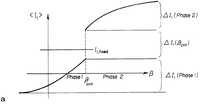
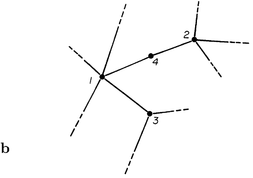
In general, a volume in action parameter space $\prod_{i}\Delta\beta_{i}(\vec{\beta_{0}})$ (i.e. in phase-diagram space) at the point $\vec{\beta_{0}}$ can be mapped into a corresponding volume in the space of extensive variables (spanned by the $I_{j}$):

$$\prod_{i}\Delta\beta_{i}(\vec{\beta_{0}})\longrightarrow\prod_{j}\Delta I_{j}(\prod_{i}\Delta\beta_{i}(\vec{\beta_{0}}))$$ (81)

This volume in $I_{j}$-space contains the combinations of values of extensive quantities that lead to parameter space values within the volume $\prod_{i}\Delta\beta_{i}(\vec{\beta_{0}})$. Generally, even an entire (single) phase corresponds to some finite volume in the space of extensive quantities spanned by the $\{I_{j}\}$. The useful feature for the purpose of fine-tuning is that, for a first order phase transition, the single points (belonging to a measure zero set) along phase borders (including the system of multiple points) correspond to a finite volume in the space of extensive quantities of size comparable to the volume associated with the dense set of points in action parameter space corresponding to the values of an entire (single) phase.

Thinking in terms of a random dynamics scenario, the values of extensive quantities $I_{j}$ are envisioned as having been randomly fixed at some set of values corresponding to a point $\vec{I_{0}}$ in the space of extensive quantities. The probability that the “coupling constants” realized in Nature fall within a small volume $\prod_{j}\Delta\beta_{j}(\vec{\beta})$ at some set $\{\beta_{0\;i}\}=\vec{\beta_{0}}$ of values is proportional to the volume $\prod_{i}\Delta I_{i}$ in the space spanned by the extensive quantities corresponding to this small volume $\prod_{j}\Delta\beta_{j}(\vec{\beta})|_{\vec{\beta}=\vec{\beta_{0}}}$.

In the case that the values in a finite volume in the space of extensive quantities all result in the action parameter values at a single point (e.g., a multiple point) greatly increases the probability that a random choice $\vec{I_{0}}$ of values in the space of extensive quantities will result in action parameter values at a phase transition. At such points (which must be first order phase transitions) the “coupling constants are “infinitely well” fine-tuned. The probability for the realization of such “infinitely well” fine-tuned values for “coupling constants” is greater the greater the “heat of fusion” at the transition.

If we think of an abstract phase diagram with a labyrinth of phase boundaries having a system of multiple points at which some number of the various phase boundaries convene, we could ascribe probabilities that one or another of the corresponding sets of values of “coupling constants” were realized in Nature according to the volume in extensive parameter space associated with these various multiple points.

The non-locality resulting from having “fixed” amounts $I_{i}=I_{i\;fixed}$ of extensive quantities in the space-time manifold is of the same type as that introduced in the water example above where the coexistence of three phases was enforced by appropriately fixing the values of $V$, $E_{TOT}$ and $n_{H_{2}O}$ so as to fine-tune the temperature and pressure to triple point values. However, non-locality that comes about in this way can essentially be “approximated away” by the standard technique of approximating a microcanonical ensemble by a canonical ensemble .

The long range correlations that strictly speaking are present in microcanonical ensembles because the total energy is “known”(thinking classically) will go unnoticed because they can be absorbed into coupling constants. In other words, this form of non-locality is acceptable because it is manifested in all space-time in the same way - namely as contributions to constants of Nature.

In implementing the 4-dimensional space-time analogy to using a canonical ensemble as an approximation to a microcanonical one, the idea[4] is to assume that the Feynman path integral of the “quantum field theory of Nature” is constrained by the requirement of fixed amounts of some (perhaps a multitude of) extensive quantities $I_{i}$ by using an action that satisfies (77). This procedure results in “coupling constants” that are maintained at critical values in a dynamical way. The mild form of non-locality discussed above (i.e., non-local terms of the Lagrange density that are reparameterization invariant) is the reason that this dynamical mechanism works in the same way everywhere in spacetime so that intensive parameters are keep at (universally) constant (critical) values.

This is also the essence of the claim to fame of Baby Universe theories: these use the effective breakdown of locality to render “coupling constants” dynamical. In the context of quantum field theory, the picture to have in mind is a universe completely permeated by a labyrinth of quantum fluctuation worm-holes. Coupling constants only “notice” the resulting non-locality in the sense that these constants are fixed as (non-local) averages over all space-time.

Back to simple model for multi-phase universe

Let us take as a prototype extensive variable the space-time integral

$$\frac{I_{2}}{V}\stackrel{{\scriptstyle def}}{{=}}\int_{V}d^{4}x|\phi^{2}(x)|\stackrel{{\scriptstyle def}}{{=}}\langle|\phi^{2}|\rangle.$$ (83)

There is one such integral for each Feynman path history of the universe. Let us assume that the value of such an integral (i.e., an extensive quantity) is fixed at some “God-given” value $\langle|\phi^{2}|\rangle_{``God"}$. This requirement

$$\langle|\phi^{2}|\rangle=\langle|\phi^{2}|\rangle_{``God"}$$ (84)

is a selection criterion that singles out a subset of all possible Feynman paths - namely those for which (84) is satisfied.

Inasmuch as this rule is a statement about the allowed values of Feynman paths when integrated from time $t_{Big\;Bang}$ to $t_{Big\;Crunch}$, it is appropriate to call this criterion (84) a non-local Law of Nature for times $t$ such that $t_{Big\;Bang}<t<t_{Big\;Crunch}$. The justification for calling (84) a non-local law is that it implements a criterion for selecting a subset of all possible Feynman paths in configuration space that is based on what will happen in the future (as well as the past of course).

This is to be contrasted to the situation for a fixed quantity $E_{TOT}/V$ in the 3-dimensional ice-water system. Here there is really no time inasmuch as the system is in equilibrium. The fixed extensive quantity $E_{TOT}/V$ is a remnant of the initial conditions of the system that (due to conservation laws) survives as an easily measured quantity in equilibrium. Fixed quantities such as $E_{TOT}/V$ in the 3-dimensional ice-water system select a subset of all possible microstate configurations in a way analogous to the manner in which the requirement (84) selects an allowed subset of all possible Feynman paths in the 4-dimensional model.

Returning now to the toy model of the universe that we want to consider, let us assume that the fixed value $\langle|\phi^{2}(x)|\rangle_{God}$ cannot be realised in all space-time (i.e., throughout the history of the universe) but instead must be realised as a “coexisting” combination of two vacua (“phases”) $\langle|\phi^{2}(x)|\rangle_{A}$ and $\langle|\phi^{2}(x)|\rangle_{B}$ corresponding to the two relative minima in the double-well potential of Sher mentioned above. We can think of a two-minima Standard Model effective Higgs field potential. For the sake of later discussion, let us assume that $\langle|\phi^{2}(x)|\rangle_{A}\leq\langle|\phi^{2}(x)|\rangle_{B}$. We shall sometimes use “us” and “other” (i.e., the vacuum we live in and some other vacuum) instead of respectively the subscripts $A$ and $B$. In what follows, spacetime averages (designated with the brackets $\langle\cdots\rangle$) that have a subscript “$A$”, “$B$”, “$us$” or “$other$” always denote values of spacetime averages that correspond to relative minima of $V_{eff}$. Hence $\langle\cdots\rangle_{A}$, $\langle\cdots\rangle_{B}$, $\langle\cdots\rangle_{``us"}$, and $\langle\cdots\rangle_{``other"}$ always denote average values $\langle f(\phi)\rangle$ of the integrand of $\frac{1}{V}\int_{V}d^{4}xf(\phi(x))$ that correspond either to true vacua or meta-stable vacua.

One possibility (the one to be considered here) would be for the fixed value of $\langle|\phi^{2}(x)|\rangle_{God}$ to be realised as a combination of the two vacua $\langle|\phi^{2}(x)|\rangle_{us}$ and $\langle|\phi^{2}(x)|\rangle_{other}$ that exist in two different time periods in the life of the universe:

$$\langle|\phi^{2}(x)|\rangle_{God}=\langle|\phi^{2}(x)|\rangle_{us}(t_{ignition}-t_{0})+\langle|\phi^{2}(x)|\rangle_{other}(t_{crunch}-t_{ignition})$$ (85)

where $t_{ignition}$ stands for “time of ignition” and denotes the time at which the transition from one vacuum to the other occurs. The scenario in which the thermodynamics of the Big Bang is such that the universe starts off in what becomes a “false” vacuum is considered in the literature[46]. This would correspond to the relative minimum in $V_{eff}$ that has the smaller value of the space-time integral $\int d^{4}x\sqrt{g(x)}|\phi^{2}(x)|$; i.e., the value $\langle|\phi^{2}(x)|\rangle_{us}$. At the time $t_{ignition}$, the transition $\langle|\phi^{2}(x)|\rangle_{us}\rightarrow\langle|\phi^{2}(x)|\rangle_{other}$ occurs.

Note that $I_{2}$ and $I_{4}$ are in this simple case a function of $t_{ignition}$ which means that $m^{2}_{Higgs}\stackrel{{\scriptstyle def}}{{=}}\frac{\partial V_{nl}(\{I_{2},I_{4}\})}{\partial I_{2}}$ is also a function of $t_{ignit}$.

Figure 11: The development of the double well potential and $m_{Higgs}$ as a function of $t_{ignition}$. Note that all the more or less randomly drawn non-locality curves intersect the “normal physics” curve near where the vacua are degenerate (i.e., the MPCP solution).

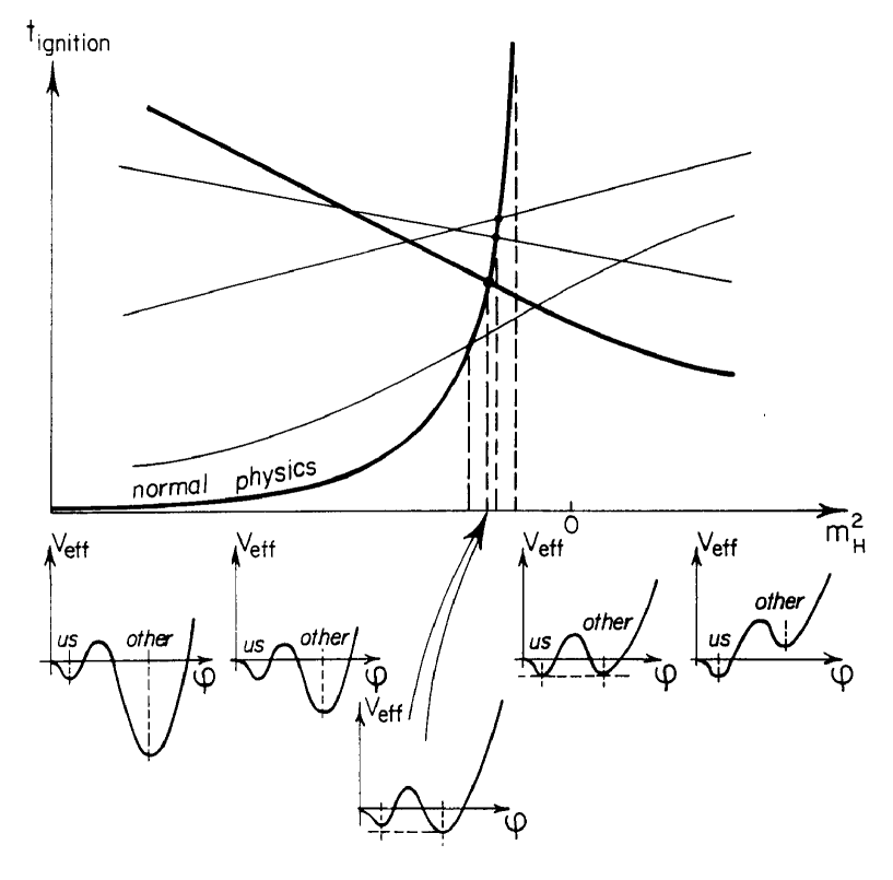
Let us first use “normal physics” to see how the relative depths of the two minima of the double well are related to $m^{2}_{Higgs}$ and to $t_{ignition}$. From the work of Sher, it can be deduced that a large negative value of $m^{2}_{Higgs}$ corresponds to the minimum at $\langle|\phi^{2}(x)|\rangle_{other}$ being deeper relative to the depth of the minimum at $\langle|\phi^{2}(x)|\rangle_{us}$ than for less negative values of $m^{2}_{Higgs}$ (see Figure 11). It can also be argued quite plausibly that a minimum at $\langle|\phi^{2}(x)|\rangle_{other}$ much deeper than that at $\langle|\phi^{2}(x)|\rangle_{us}$ would correspond to an early (small) $t_{ignition}$ inasmuch as the “false” vacuum at $\langle|\phi^{2}(x)|\rangle_{us}$ is very unstable. However, as the value of the potential at $\langle|\phi^{2}(x)|\rangle_{other}$ approaches that at $\langle|\phi^{2}(x)|\rangle_{us}$, $t_{ignition}$ becomes longer and longer and approaches infinity as the depth of the wells at $\langle|\phi^{2}(x)|\rangle_{us}$ and $\langle|\phi^{2}(x)|\rangle_{other}$ become the same; it may be that $t_{ignition}$ becomes infinite before the minimum at $\langle|\phi^{2}(x)|\rangle_{us}$ becomes as deep as the minimum at $\langle|\phi^{2}(x)|\rangle_{other}$. The development in the form of the double well potential as $t_{ignition}$ becomes larger corresponds to less and less negative values of $m^{2}_{Higgs}$. The development of the double well potential and $m^{2}_{Higgs}$ as a function of $t_{ignition}$ is illustrated in Figure 11.

In the simple cosmological model being considered, it is readily seen that the “coupling constant” $m^{2}_{Higgs}$, regarded as function of $t_{ignition}$, depends on the future as well as the past. Note that the larger the difference $|\langle|\phi^{2}(x)|\rangle_{other}-\langle|\phi^{2}(x)|\rangle_{us}|$ the greater the dependence of $I_{2\;``God"}\stackrel{{\scriptstyle def}}{{=}}\langle|\phi^{2}(x)|\rangle_{``God"}$ on $t_{ignition}$ (this corresponds to a large heat of fusion in the ice-water analogy). If $\langle|\phi^{2}(x)|\rangle_{us}=\langle|\phi^{2}(x)|\rangle_{other}$, the dependence on $t_{ignition}$ disappears as does the non-locality in the theory.

Prediction of top quark and Higgs masses

In very recent work[47], our multiple point criticality principle has been used to predict the masses for the top quark and the Higgs mass. This is done by making the the multiple point criticality optimally effective. First the MPCP is assumed using the formulation that the two minima - denoted $V_{us}$ and $V_{other}$ - of the Standard Model Higgs field potential (with one-loop corrections) are degenerate: $V_{us}=V_{other}$. Secondly, it is assumed that $|\langle|\phi^{2}(x)|\rangle_{other}-\langle|\phi^{2}(x)|\rangle_{us}|$ is as large as “possible” subject to the constraint that we should stay below the Planck scale. This insures the largest possible number of combinations of fixed extensive quantities that are not realisable as a single phase (or, more generally, not realisable with a smaller number of phases than are present at the multiple point). The analogy to this assumption in the example above with water (in which ice, liquid, and vapour coexist at the triple point) would be that Nature had chosen large values for the heats fusion, vaporisation, and sublimation.

In the work[47] in which the top quark and Higgs masses are predicted, the authors take $|\langle|\phi^{2}(x)|\rangle_{other}-\langle|\phi^{2}(x)|\rangle_{us}|$ as being of order unity in Planck units. This amounts to taking the vacuum expectation value of $|\langle|\phi^{2}(x)|\rangle_{other}$ to be of order unity in Planck units and $\langle|\phi^{2}(x)|\rangle_{us}|$ (the vacuum corresponding to physics as we humans know it) to be as determined by the Standard Model (which turns out to be very small in terms of Planck scale units). This amounts having the minimum $V_{other}$ at the Planck scale; this assumption is consistent with Planck scale units being regarded as important in fundamental physics and at the same time maximises the probability that the intensive quantities Higgs mass and top quark mass acquire values dictated by the MPCP fin-tuning mechanism. This follows because even randomly chosen values of $\langle\phi^{2}(x)\rangle$ are not likely to fall outside the interval $|\langle|\phi^{2}(x)|\rangle_{other}-\langle|\phi^{2}(x)|\rangle_{us}|$ that is of order unity in Planck scale units.

This assumption of maximally effective MPCP fine-tuning leads to remarkably good predictions for the top quark and Higgs masses. The prediction is $(M_{t},M_{H})=(173\pm 4,\;\;135\pm 9)$ GeV. The authors of this work[47] conclude that if this very good prediction of the top quark mass and reasonable prediction for the expected Higgs mass are not regarded as accidental, one is essentially forced to accept the validity of the multiple point criticality principle fine-tuning mechanism as well as the minimal standard model (at least as far as the top quark and Higgs interactions are concerned). The latter implies that super-symmetry would not be allowed.

Avoiding paradoxes arising from non-locality

Figure 12: Many non-locality curves could lead to paradoxes similar to the “matricide” paradox. Such paradoxes are avoided if the value of $m_{Higgs}$ is fine-tuned to the multiple point critical value.

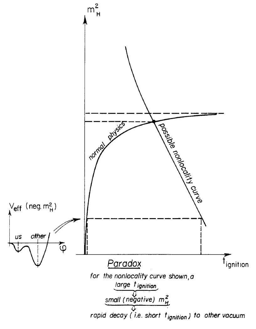
In general the presence of non-locality leads to paradoxes. While the form that the non-local action (or potential $V_{nl}$ in this discussion) is, at present at least, unknown to us, we can make some guesses as to its form. These guesses could correspond to the non-locality curves in Figure 11. In particular, non-locality curves having a negative slope as a function of $t_{ignition}$ lead to paradoxes in the following manner. Consider specifically the non-locality curve in Figure 12. Now let us make the assumption that $t_{ignition}$ is large and see that this leads to a contradiction. Assuming that $t_{ignition}$ is large, it is seen from the non-locality function in Figure 12 that this implies that $m^{2}_{Higgs}$ has a large negative value. But a large negative value of $m^{2}_{Higgs}$ corresponds to a vacuum $\langle|\phi^{2}(x)|\rangle_{us}$ that is very unstable and hence to a very short $t_{ignition}$ (corresponding to a rapid decay to the stable vacuum $\langle|\phi^{2}(x)|\rangle_{other}$). So the paradox appears: the assumption of a large $t_{ignition}$ implies a small $t_{ignition}$. This is very much akin to the “matricide” paradox encountered for example when dealing with “time machines”. It is well known[48, 49, 50] that Nature avoids such paradoxes by choosing a very clever solution in situations where these paradoxes lure.

In the case of the paradoxes that can come about due to non-locality of the type considered here, the clever solution that Nature uses to avoid paradoxes is that of obeying the Principle of Multiple Point Criticality[2]. This corresponds to the intersection of the “normal physics” curve and the “non-locality” curve in Figure 12. This point corresponds to a value of $m^{2}_{Higgs}$ for which the vacua at $\langle|\phi^{2}(x)|\rangle_{us}$ and $\langle|\phi^{2}(x)|\rangle_{other}$ are (almost) degenerate. This is equivalent to being at the multiple point. The paradox is avoided by taking the multiple point value of $m^{2}_{Higgs}$. But at the multiple point, an intensive parameter has its value fine-tuned for a wide range of values for the quantity conjugate to this intensive quantity. Fine-tuning is to be understood as a consequence of Nature’s way of avoiding paradoxes that can come about due to non-locality.

It should be pointed out that the paradox-free solution corresponding to the intersection of the two curves in Figure 12 occurs for a value of $m^{2}_{Higgs}$ corresponding to “our” vacuum at $\langle|\phi^{2}(x)|\rangle_{us}$ being very slightly unstable. The value of $m^{2}_{Higgs}$ corresponding to the vacua at $\langle|\phi^{2}(x)|\rangle_{us}$ and $\langle|\phi^{2}(x)|\rangle_{other}$ being (precisely) degenerate is slightly less negative than that corresponding to the multiple point value of $m^{2}_{Higgs}$ at the intersection of the curves.

It is very satisfying from the point of view of Random Dynamics to see that the the multiple point value of $m^{2}_{Higgs}$ is very insensitive to which “guess” we use for the non-local action. Indeed all the “non-locality” curves in Figure 12 intersect the “normal physics” curve at values of $m^{2}_{Higgs}$ that are tightly nested together. The reason for this is that the $m^{2}_{Higgs}$ is a very slowly varying function of $t_{ignition}$ as $m_{Higgs}^{2}(t_{ignition})$ approaches the value corresponding to degenerate vacua. The more nearly parallel the “normal physics” and the “non-locality” curves at the point of intersection, the less are the (paradoxical) effects of non-locality. For a point of intersection at values of $t_{ignition}$ sufficiently large that $m^{2}_{Higgs}(t_{ignition})\approx m^{2}_{Higgs}(\infty)$), the non-locality effects disappear as the curves become parallel since both curves become independent of $t_{ignition}$. If the curves were parallel, there would also be the possibility that they don’t intersect in which there would be no “miraculous solution” that could avoid the paradoxes imbued in having non-locality.

If the interval $|\langle|\phi^{2}(x)|\rangle_{other}$-$\langle|\phi^{2}(x)|\rangle_{us}|$ is large (e.g. of the order of the largest physically conceivable scale (Planck?) if tuning is to be maximally effective) and if $\langle|\phi^{2}(x)|\rangle_{``God"}$ falls not too close to the ends of this interval, then $t_{ignition}$ will be something of the order of half the life of the universe. Actually, the approximate degeneracy of the vacua $\langle|\phi^{2}(x)|\rangle_{other}$ and $\langle|\phi^{2}(x)|\rangle_{us}$ may be characteristic of the temperature of the post-Big Bang universe in the present epoch and not characteristic of the high temperature that prevailed immediately following the Big Bang. Such a much higher temperature universe might very plausibly have favoured the vacuum at $\langle|\phi^{2}(x)|\rangle_{us}$ very strongly at the expense of the “phase” corresponding to the $\langle|\phi^{2}(x)|\rangle_{other}>\langle|\phi^{2}(x)|\rangle_{us}$. This could be explained as being due to the fact that at high temperatures, the free energy is considerably less than the total energy if the entropy is large enough. A phase with a large number of light particles - for example a Coulomb-like vacuum such as the “us” phase in which we live - could very plausibly be so strongly favoured at high temperatures that other phases - for example the “other” vacuum - simply disappeared at the high temperature of the universe immediately following the Big Bang.

If this were to have depleted the universe of the phase $\langle|\phi^{2}(x)|\rangle_{other}$ at high temperatures, it would indeed be difficult to re-establish it in a lower temperature universe even if the vacuum $\langle|\phi^{2}(x)|\rangle_{us}$ were only meta-stable and $\langle|\phi^{2}(x)|\rangle_{other}$ were were the true vacuum at the lower temperature. Such an exchange of the true vacuum is indeed a possibility in going to lower temperatures inasmuch as the difference between the total energy and the free energy decreases in going to lower temperatures. Accordingly this difference becomes less effective in favouring a Coulomb-like phase at the expense of a phase with heavy particles.

On the other hand, the value of $\langle|\phi^{2}(x)|\rangle_{``God"}$ can easily (i.e. as a generic possibility) assume a value that requires the the universe to be in the “phase” $\langle|\phi^{2}(x)|\rangle_{other}$ during a sizeable period of its life if the universe is to have multiple point parameters in the course of its evolution (as required for avoiding the paradoxes that accompany non-locality). How can Nature overcome the energy barrier that must be surmounted in order to bring about the decay of the slightly unstable (false) vacuum at $\langle|\phi^{2}(x)|\rangle_{us}$ to the vacuum at $\langle|\phi^{2}(x)|\rangle_{other}$? Even producing just a tiny “seed” of the vacuum $\langle|\phi^{2}(x)|\rangle_{other}$ would be very difficult. What miraculously clever means can Nature devise so as to avoid deviations from a multiply critical evolution of the universe? One extraordinarily ingenious master plan that Nature may have implemented has recently been proposed by Holger Bech Nielsen. Maybe life was created with the express “purpose” of evolving some (super intelligent?) physicists that could ignite a “vacuum bomb” by first creating in some very expensive accelerator the required “seed” of the “correct” vacuum $\langle|\phi^{2}(x)|\rangle_{other}$ that subsequently would en-gulf the universe in a (for us) cataclysmic transition to the “other” phase thereby permitting the continued evolution of a “paradox-free” universe!

3.2.4 Two-position fields/particles replicated at one position

In Sections 3.2.1 and 3.2.2 we have suggested that, if fields are defined the usual way as functions of space-time points (and if for simplicity short distance non-localities are ignored), we can interpret long distance non-locality that is independent of space-time as being incorporated into the laws of Nature rather than being observable in some offensive way. However, having once relinquished the principle of locality in this mild ontological sense, there is no longer any compelling reason to assume that fields depend on just one space-time point! Rather it becomes quite natural to contemplate the possibility of having, for example, a field $\phi(x,y)$ that depends on two space-time points $x=x_{\mu}$ and $y=y_{\mu}$. If we for simplicity take $\phi(x,y)$ as a scalar field, it transforms under reparameterization transformations (i.e., diffeomorphisms), in both $x$ and $y$:

$$\phi\rightarrow\phi^{\prime}\;\;\mbox{where}\;\;\;\phi^{\prime}(x^{\prime},y^{\prime})=\phi(x(x^{\prime}),y(y^{\prime})).$$ (86)

Physically a field such as $\phi$ is just a function of a couple of space-time points regarded as abstractly defined (i.e. coordinate independent) events.

The integrals that can be used for constructing a nonlocal but still reparameterization invariant action, depending on such double-position fields $\phi(x,y)$, can hardly be imagined to be anything but double integrals of the form

$$\int d^{4}x\int d^{4}y{\cal F}(\phi(x,y),\phi(x),\phi(y),\partial\phi(x,y)/\partial x^{\mu},...).$$ (87)

Roughly such a model can be thought of as one in which space-time is 8-dimensional rather than just 4-dimensional but in which there are two types of particles:

a) “ordinary” particles (or fields) having only one position and really only depending on four out of the eight coordinates, e.g. on $x$ but not on $y$.

and

b) “double position particles (or fields)” (e.g., $\phi(x,y)$) that can take values in the entire 8-space.

In practice we presumably have something we may call “vacuum” for both sorts of fields: vacuum values in the classical approximation are constant (zero say) over most combinations of $x$ and $y$. Assuming “we” humans are primarily composed of “ordinary” particles, we could not readily interact with the Fourier components of the $\phi(x,y)$ field unless these components have zero momentum along either $x$ or $y$. Genuine excitations of $\phi(x,y)$ locally in the 8-dimensional space can only occur by interaction of two ordinary particles and therefore are presumably rather suppressed. This makes it very difficult in practice to discover the non-locality related to the two-position fields, unless there are some huge amounts of matter in 8-space so to speak.

If reparameterization invariance is not to be broken spontaneously, we must have fields - for example $\phi(x,y)$ -that are constant in all 8-space points $(x,y)$ except along the diagonal $x=y$ (and, presumably, infinitesimally close to $x=y$). However, the absence of non-locality that we experience phenomenologically is probably insured if there is not spontaneous breakdown under reparameterizations in a local region. So if the reparameterization in one neighbourhood differed from that prescribed by reparameterization invariance at another very far removed region, this might well not be observed as a breaking of locality. So a priori it would not be forbidden phenomenologically if the field $\phi(x,y)$ takes on some other values (i.e., departing from the almost everywhere dominant constant vacuum value) along a thin band representing a graph of a function yielding $y$ as function of $x$. We assume that the structure is the same everywhere along this band so that there is still reparameterization invariance under the special type of transformation that transforms the $x$ and $y$ at a point $(x,y)$ in the band in the same way. Field configurations corresponding to this band make up a 4-dimensional manifold in the 8-dimensional $(x,y)$ space, along which there can be a systematic communication between a space-time point $x$ and its image $y$.

If we had efficient communication by non-locality between say $x$ and $y$ due to the above-outlined spontaneous breakdown of reparameterization invariance, one can enquire as to whether this effect would be perceived as a breaking of locality. Probably not: rather we would interpret the related space time points - the ones with $(x,y)$ on the band - as representing different degrees of freedom at a single space-time point $x$ say. Because we would experience the space-time point $x$ and its image $y$ as the same space-time point, locality is effectively restored. Concurrent with this, we would experience a replication of the field degrees of freedom at one space-time point! In Nature we seem to see a 3-fold replication with respect to the fermions, in the sense that we observe three generations. A tripling of the number of fields can easily be achieved with (just) two-position fields that are applied a couple of times: the two-position field may have several “bands” as proposed, so that one point - $x$ say - can be connected to several (e.g. two) far away points $y$, by two different bands in the same $\phi(x,y)$-field.

Indeed, in the experimentally supported Standard Model, we find a trinity of similar (but not exactly replicated) field types: the three generations of quarks and leptons! But the three generations found in Nature are not exact replicas of each other, as one at first might expect if these truly represented particles of the same sort just at different points in space and time. However these generations may correspond to superpositions of states at different related space-time points; there is also the possibility of some sort of (later) spontaneous breakdown of the symmetry between the different related space time points. There is therefore no necessity for perfect symmetry between the different generations, in order to uphold the interpretation that these are due to the non-locality with spontaneously broken reparameterization symmetry.

Moreover, we would expect that a 3-fold (approximate) replication mechanism due to non-locality would not only triple the quark and lepton fields but also the boson fields! In fact, such a tripling of boson fields is an intrinsic feature of our long standing $SMG^{3}$ “anti-grand unification” gauge group model. In this model, we predict that the values of the fine-structure constants at the multiple point of the phase diagram for the gauge group $SMG^{3}$ should agree with experimental values. For the moment let us content ourselves with the observation that non-locality can easily lead to a picture in which not only the fermions are tripled but also, essentially unavoidably, the bosons. That is to say, we would predict, roughly speaking, 3 photon-types, three $W^{+}$’s, three $W^{-}$ ’s, three $Z^{0}$’s, and 24 gluons. There may also be some predicted but not observed gauge bosons (and presumably even more Higgses or replacements for them) that would need to be given large masses.

3.2.5 Concluding remarks on non-locality and MPC

Relinquishing strict adherence to the principle of locality has several attractive features from a theoretical point of view. In other work[29, 26, 7] we have in the spirit of Random Dynamics also investigated the possibility of removing this principle from the list of initial assumptions necessary for constructing a fundamental theory.

Starting with the problem of the cosmological constant being almost zero - from a Planck scale point of view at least - we have argued that there should be a breakdown of the principle of locality for field interactions from a fundamental point of view. We have also argued that if fundamental physics obeys the multiple point criticality principle in 4-dimensions, non-locality is implied (at least in the mild form in which reparameterization invariance remains intact) inasmuch as it seems difficult to find another explanation if one accepts the phenomenological validity of the MPCP. Going the other way, we have also argued that if non-locality is an inherent feature of fundamental physics, the solution whereby paradoxes due to non-locality are avoided coincides with the choice of the multiple point values of coupling constants.

As already mentioned, it appears that a theory with non-locality (that retains reparameterization invariance) or, equivalently, a theory for which the MPCP is valid provides a promising approach to explaining a series of fine-tuning problems. The principle of multiple point criticality - which essentially asserts the coexistence of a number of phases - leads to such an impressive number of good predictions for fine-tuned quantities that one is almost forced to take it seriously!

Essentially all of the well known fine-tuning mysteries in high energy physics are potentially solved: 1) the vanishing of the dressed cosmological constant; 2) the small Higgs field expectation values and masses; 3) the hierarchy of quark and lepton masses; 4) strong CP conservation and 5) the multiple point values of fine-structure constants.

The values obtained assuming the MPCP for the three Standard Model gauge couplings are discussed at length elsewhere in this thesis. The manner in which the MPCP might solve the mysteries of the first four fine-tuning enigma are briefly mentioned now.

1. Cosmological constant $\Lambda_{eff}=0$ at transition from finite to infinite universe

   According to the multiple point criticality model for fine-tuning, one should expect to find the fine-tuned parameters observed in Nature at parameter values that coincide with MPCP values. Since the cosmological constant value $\Lambda_{eff}=0$ corresponds to the border between finite and infinite space spheres (universes), it is not surprising that computer simulations[51, 52] of quantum gravity indicate singular behaviour at the value $\Lambda_{eff}=0$ for the cosmological constant. We can therefore claim that the phenomenologically indicated value $\Lambda_{eff}=0$ coincides with the MPCP prediction for the value of the cosmological constant.

2. Our “unfortunate ” prediction of the Higgs mass

   A promising proposal for the explanation of the fine-tuning problem of the expected small value of the Weinberg-Salam Higgs mass (compared say to the Planck scale) is at hand if the multiple point criticality idea for gauge couplings is assumed to be valid in a slightly extended form that requires not only that a maximum number of Coulomb-like and confinement-like “phases” (i.e. partially confining phases ) be accessible at the multiple point (by making infinitesimal changes in the multiple point coupling values) but also that (Planck scale) multiple point parameters should be at the border between Higgsed and un-Higgsed phases. At such boundaries there is a change of sign in $m_{Higgs}^{2}$ which, for transitions that are not too strongly first order, would imply that values of $m_{Higgs}^{2}$ relative to the Planck scale are strongly suppressed. So in a certain sense, our fine-tuning model explains the physical fine-tuning problem related to the so-called hierarchy problem. The hierarchy problem might then be said to be Nature’s way of telling us that the Yang-Mills vacuum is very close to a Higgs phase boundary! It should be pointed out that the need for solving this problem has often been used to argue for super-symmetry.

   Let us elaborate briefly on this a priori promising but de facto experimentally refuted approach. Using one-loop corrections, logarithms can get introduced into the condition for the coexistence of phases in such a way that the Higgs mass, or equivalently the Higgs field expectation value appears only in a logarithm in the equation imposing the coexistence of the Weinberg Salam Higgs phase and the unbroken phase (in which $W^{+}$, $W^{-}$ and $Z^{0}$ would be massless). In this event, we can argue that the fine-tuning mystery of why the scale of the Higgs expectation value is so very low compared say to the Planck scale is solved: once the ratio is determined by its logarithm, it can easily become very large.

   The calculation of what happens when we impose the requirement of the equality of the Higgs field potential depths for the two minima corresponding to the mentioned phases - the Higgs and the unbroken (= Coulomb) phase - has in fact already been performed; this specially adjusted Higgs potential corresponds to the Linde-Weinberg bound[53, 54] which is slightly different that the better known Coleman-Weinberg bound[55]. In the Linde-Weinberg bound, the Higgs bare mass is fine-tuned to the requirement that the two minima be equally deep. This is precisely what our prediction using multiple point criticality (or fundamental non-locality) would suggest: we predict the Linde-Weinberg situation as the solution to the problem of why the Higgs field expectation value is so small. Indeed, in the Linde-Weinberg situation, the vacuum expectation value of the Higgs field is obtained from a logarithm and in this way comes to deviate exponentially from the input mass. In the philosophy of a fundamental scale, we would of course take the input mass to be at the Planck scale (or whatever the fundamental scale is taken to be). This looks wonderful at first: we have solved the problem of the small Higgs expectation value by postulating fundamental non-locality! The technical hierarchy problem, that, in going to different orders in perturbative calculations, includes quadratic divergences (if you do not have super-symmetry at least) which are expected to be of the order of the cut-off scale, is now argued away. This is done by claiming that in going to different orders in the perturbative calculations, we should for each order recalculate the amount of space-time volume which is in the unbroken phase (and the amount which is in the Higgs phase). After this recalculation - which is not really performed inasmuch as we do not actually know the non-local action - we find that we have just to use the Linde-Weinberg situation in which case the Higgs mass and expectation value are not renormalised away.

   However, the Linde-Weinberg bound does not agree well with experiment. The prediction obtained from the requirement of remaining within this bound - this must also be taken as our prediction from non-locality - is a Higgs mass which, using the usual expectation value known from experimental weak interactions, turns out to be 7.8 GeV and, in the same connection, a top-quark mass of less than about 90 GeV. This is a failure of our model that might be resolvable if there were several Higgs fields in which case the simple Linde-Weinberg calculation would not hold true. With this scenario, one could hope to retain the exponential behaviour of the Higgs field expectation value and thereby still solve the hierarchy-related problem of why the Higgs particle is so light.

   Another possible scenario would be that Nature ends up at a point in the multiply critical manifold (presumably of high dimension) at which phase transitions are maximally first order. In this picture, $m^{2}_{Higgs}$ becomes small by using the well-known two-minima Higgs field potential of the pure Standard Model with one-loop corrections[46] in conjunction with the MPCP fine-tuning mechanism. This latter states that the Higgs field minima should be degenerate (i.e., have identical energy densities) and furthermore, that the generic probability for having a universe that can only be realized with two or more coexisting phases should be maximised (maximum “heat of melting”). This latter is implemented in[47] by postulating that one of the minima is at the largest thinkable energy - the Planck scale. This is tantamount to taking the “heat of melting” to be of order unity in Planck scale units; it is then generically unlikely that a universe can be realised as a single phase. The two minima of the degenerate vacua of the Higgs field potential get in this way separated by energies that differ maximally; i.e., of order of unity in Planck units. By assuming that this gap in energy is as large as possible, it is almost insured that even randomly chosen values of “extensive variables” (e.g., energy) will fall within this gap and that the conjugate intensive quantities (e.g., Higgs mass and top quark mass) will accordingly be fine-tuned. This implementation of the multiple point criticality fine-tuning mechanism yields extremely good predictions[47] for the top quark mass and the expected Higgs mass. This has been discussed in Section 3.2.3.

   Furthermore, by postulating that Nature seeks out multiple point criticality at maximally first order transitions (on for example a multi-dimensional multiply critical surface), we might also alleviate the universality problem inherent to first order transitions[56] inasmuch as the requirement of maximal first-orderness might place us at a unique position in the multiply critical manifold in parameter space. This could lead to unique values of continuum couplings.

3. Mass Hierarchies of Quark-Lepton Generations
   As one of the fine-tuning mysteries we also count the question of why the masses for most quarks and leptons are so small compared to the weak interaction scale, which is the mass you would expect if the Yukawa couplings were simply of order unity [5, 6]. The explanation suggested is that, in the physics at the fundamental scale, there are some Higgs fields that get relatively small expectation values, much in analogy to the above speculation about the Weinberg-Salam Higgs field. They might even easily be exponentially light, due to the fact that their masses are determined via a logarithm. But even just the presence of the phase transition makes the Higgs masses small. After all, it is at a transition between positive and negative mass squared that we have the boundary between the Higgsed and the Coulomb phases. This then means that the transitions between left and right handed components of fermions, which need such Higgses for their occurrence, are suppressed. Recent work [57, 58, 59] explores the mass hierarchy of fermions (leptons and quarks) as a consequence of Higgsed gauge symmetries that are only weakly broken, due to the Higgs fields having only “small” expectation values. Such a mechanism can rather naturally explain the large gaps between the generations in the mass spectrum.

   From the point of view of a very general picture with approximately conserved quantum numbers, searches have been made for clues as to which approximately conserved gauge quantum numbers should exist beyond the Standard Model. Using the extra quantum numbers in the $SMG^{3}$ model (that is used here to in connection with our MPCP predictions of fine-structure constants) leads to a rather natural explanation of the generation mass gaps. However, a problem is encountered in getting the top quark mass sufficiently heavy compared to the bottom quark and $\tau$ lepton masses. However adding a fourth Abelian gauge group $U(1)_{f}$ helps[57, 58, 59].

4. Strong CP-conservation also at a junction of phases

   Yet another fine-tuning problem is the strong CP-problem. The $\Theta_{QCD}$ dependence of the first order de-confining phase transition has recently been studied[60]. It is found that in the continuum limit there is a critical point at $\Theta_{QCD}=0$, where the confinement phase corresponding to $\Theta_{QCD}=0$ meets the “Higgs” phase corresponding to $\Theta_{QCD}\neq 0$. It then follows, assuming that QCD is in the confinement phase, that $\Theta_{QCD}=0$ and CP is conserved by the strong interactions. However, from our point of view, we look for a more “ontological” type of solution and do not accept that Nature at the bare level should be precisely renormalised to, for example, reveal the confining phase of long distance QCD. We can nevertheless, in the spirit of our multiple point principle above, use the phase diagram of [60] to suggest the possibility that $\Theta_{QCD}=0$ can be characterised as a meeting point for phases. Therefore, even the strong CP-problem of why $\Theta_{QCD}$ is so small can find an explanation derivable from the coexistence of phases in the same spirit as our solution of the other fine-tuning problems.

3.3 A speculative alternative proposal for the stability of the multiple point

The most current and probably most eloquent explanation for Nature’s affinity for the multiple point stems from the apparent necessity of having long distance (diffeomorphism invariant) nonlocal interactions if the fine-tuning of physical constants is to be dynamical (discussed in Section 3.2). However, an earlier pursuit of a theoretical explanation for why the multiple point should be realised in Nature has some merits. This proposal of a mechanism for the stability of the multiple point (outlined in more detail in Appendix LABEL:specproapp) assumes a nonlocal lattice gauge glass with a random plaquette action (e.g.; an action with quenched random values for character expansion parameters). Here “non-locality” is restricted to fundamental scale distances: action terms for Wilson loops of extent $A$ very large compared to the lattice constant $a$ are effectively nonlocal as seen from scales in the intermediate length range $[a,A]$. We define gauge couplings that run due to the inclusion of successively larger Wilson loops in going towards the infrared. The effect of these terms on the running of the couplings is describable by an extra term in the Callan-Symanzik $\beta$-function. The inclusion of these glassy nonlocal action terms in such a generalised $\beta$-function (really a multicomponent vector of generalised $\beta$-functions) is in addition to but opposite in sign to the normal Yang-Mills renormalization group contribution. It is argued that rapid variations in the generalised $\beta$-functions at the multiple point can easily lead to zeros of these $\beta$-functions close to the multiple point. It is estimated that already at energies near the Planck scale the running plaquette action parameter values are presumably very close to those of the “infrared stable” fixed point zeros of the generalised $\beta$-functions which in turn are close to the multiple point (see Appendix 11.5).

theph.tex 31 May 96 alf

4 The phases of a non-simple gauge group

4.1 Features of the phases that can convene at the multiple point

Since it is postulated that Nature seeks a special point in plaquette action parameter space - the multiple point - where many “phases” come together, it is necessary to clarify what is meant by these “phases” as well as how such different “phases” are distinguished. This is the purpose of this Section.

First it should be made clear that when referring to phases of groups at the Planck scale, it is phase transitions between what are usually referred to as lattice artifact “phases”. Distinguishing quantitatively different physical behaviours - here referred to as “Higgs-like”, “Coulomb-like” and “confinement-like phases” - at the lattice scale (here taken as the Planck scale) is motivated from results[61, 62, 63, 64, 65] obtained using the mean field approximation $(MFA)$ which intrinsically distinguishes phases on the basis of the qualitative differences in the physics that are discernible at the scale of the lattice. All “phases” involving non-Abelian degrees of freedom will of course, for sufficiently long distances, turn out to be confining with no long range correlations (corresponding to finite glue-ball masses) when, as is the case in this section, matter fields are ignored.

An important feature of the phases of interest here is that they be identifiable at the scale of the lattice. The following discussion of some qualitative features of such phases motivates the more or less well known fact that transitions between the lattice artifact phases of interest to us are first order transitions (at least near the multiple point). Let us write the logarithm of the partition function as $\log Z\propto V_{tot}\cdot\log f(\beta)$ where $V_{tot}$ is the geometrical volume of the system and $f(\beta)\stackrel{{\scriptstyle def}}{{=}}\frac{1}{V_{tot}}\log Z$ is the free energy density. As $Z$ is essentially the product of the average height $\langle e^{S_{action}}\rangle$ of the distribution of plaquette variables times the average width $W(\beta)$ of this distribution, we can write $f(\beta)=\langle s_{action}\rangle+s_{entropy}$ where $\langle s_{action}\rangle\stackrel{{\scriptstyle def}}{{=}}\frac{1}{V_{tot}}\langle S_{action}\rangle$ and $s_{entropy}\stackrel{{\scriptstyle def}}{{=}}\frac{1}{V_{tot}}\log W(\beta)$.

Let us clarify the properties required of two phases - call them phases $I$ and $II$ - in order that they be distinguishable using a small geometric sampling volume of the order of a few lattice cubes. The hope for being able to do this lies in not having much overlap in the regions of configuration space that are appreciably populated in different phases . This being the case, it is meaningful to introduce free energy density functions $f_{I}(\beta)$ and $f_{II}(\beta)$ that very much dominate respectively in the phases $I$ and $II$:

$$f(\beta)\approx\left\{\begin{array}[]{l}f_{I}\mbox{ in phase I}\\ f_{II}\mbox{ in phase II}\end{array}\right.$$ (88)

which corresponds to a partition function $Z$ that approximately factorizes with one factor for each of the two phases $I$ and $II$:

$$Z\approx Z_{I}(\beta)+Z_{II}(\beta).$$ (89)

The disjointness of the regions of configuration space appreciably populated in phases $I$ and $II$ is tantamount to requiring that the quantity

$$\log(\frac{Z_{I}(\beta)}{Z_{II}(\beta)})=V_{tot}(f_{I}(\beta)-f_{II}(\beta))$$ (90)

be very large or very small depending on whether we are in phase $I$ or $II$ (assuming that we are sufficiently far removed from the phase boundary where by definition $\frac{Z_{I}(\beta)}{Z_{II}(\beta)}=1$). The relation (90) is equivalent to saying that if, in going from phase $I$ to $II$, this quantity that contains $V_{tot}$ as a factor changes by a large amount, a change could also be detected using a smaller volume (e.g., a lattice scale volume $V_{lattice\;scale}$).

This scenario relies in an essential way on the assumption that the quantity $f_{I}(\beta)-f_{II}(\beta)$, which vanishes at the phase boundary, rapidly becomes large or small in going to parameter values $\beta$ removed from the boundary. This in turn relies on having to a good approximation a discontinuous change at the phase boundary in the configuration space appreciably populated by the two phases. This would be reflected as a discontinuity at the boundary in the entropy

$$\Delta s_{entropy}=s_{I,\;entropy}(\beta_{crit}+\epsilon)-s_{II,\;entropy}(\beta_{crit}-\epsilon).$$ (91)

Such a discontinuity can come about at the phase boundary if there is a compensating jump in the average plaquette action

$$\Delta\langle s_{action}\rangle=\langle s_{I,\;action}(\beta_{crit}+\epsilon)\rangle-\langle s_{II,\;action}(\beta_{crit}-\epsilon)\rangle.$$ (92)

in accord with having (by definition) $f_{I}=f_{II}$ at the phase boundary; i.e., in the limit $\epsilon\rightarrow 0$, we must have

$$0=\log f_{I}(\beta_{crit}+\epsilon)-\log f_{II}(\beta_{crit}-\epsilon)=\Delta\langle s_{action}\rangle-\Delta s_{entropy}$$ (93)

But the average plaquette action is essentially the derivative of $\log Z$ w.r.t $\log\beta$ so a jump in $\langle s_{action}\rangle$ is tantamount to a discontinuity in $\frac{\partial\log Z}{\log\beta}$ which is of course the defining feature of first order phase transitions. In fact it is known from Monte Carlo calculations based on lattice gauge theories that phase transitions at the multiple point are first order. So the idea of distinguishing lattice artifact phases at the scale of the lattice is not inconsistent with known results.

However, determination of gauge couplings based on first order phase transition are intrinsically plagued by problems of non-universality. From this point of view, second order phase transitions would be preferable. However, it is rather meaningless to talk about second order phase transitions at a given scale. The phases separated by a second order phase transition are defined relative to distinct (different) fixed points in parameter space; a particular phase is identified by which fixed point the running coupling(s) converge to in the long wavelength limit. That second order phase transitions can first be identified in the limit of long wavelengths can be understood intuitively when it is recalled that the derivative of $\log Z$ w.r.t. $\beta$ is continuous at the phase boundary of a second order phase transition. It is therefore difficult to avoid overlap in the regions of configuration space appreciably populated by the two phases. Hence the quantity $f_{I}(\beta)-f_{II}(\beta)$, which can be expected to be large for first order transition, become smaller (and a more poorly defined quantity) in the transition from a first order to second order phase transition - even for points in the phases $I$ and $II$ far removed from the phase boundary. In this case, the condition $\frac{Z_{I}(\beta)}{Z_{II}(\beta)}\neq 1$ (which really has no meaning for a fully second order phase transition) that is necessary for being able to see that there are two phases requires a larger and larger sample volume $\approx V_{tot}$. This is another way of saying that we have to take a long wavelength limit in order to see a second order phase transition.

For small sampling volumes $V_{sample}$, first order phase transitions dominate completely over second order transitions in determining the physically realized phase boundary.

At the multiple point of a phase diagram for a lattice gauge theory, the different lattice artifact phases are presumably separated by first order phase transitions and accordingly are distinguishable using a small sampling volume which is assumed to be of the order of the Planck scale lattice. Such phases are therefore completely governed by which micro (e.g. Planck scale) physical fluctuation patterns yield the maximum value of $\log Z$. Qualitatively different short distance physics could consist of different distributions of group elements along various subgroups or invariant subgroups of the gauge group for different regions of (bare) plaquette action parameter space. It is therefore the physics at the scale of the lattice that is of interest because it is lattice scale physics that dominates the different $\log Z$ ansatz that prevail (i.e., are maximum) in different parameter space regions separated by first order transitions. However, this does not mean that longer distance behaviour is unchanged in passing from one “phase” to another. As an example, consider the string tension at the transition between two different lattice scale phases that both really correspond to confining phases in the usual sense: in what we designate as confining in the mean field approximation ($MFA$) or “confinement at the lattice scale”, the string tension has an order of magnitude given by dimensional arguments from the lattice. On the other hand, in what we call the “Coulomb phase at the lattice scale”, or the Coulomb phase in the $MFA$ approximation, the string tension is much smaller; i.e,. smaller by an exponential factor.

4.2 Goal: the classification of the phases of the vacuum for a lattice gauge theory with non-simple gauge group

Now we want to assign names to the different lattice artifact phases, i.e., qualitatively different physical behaviours of the vacuum of a lattice gauge theory at the lattice scale. The different phases that are possible depend on the gauge group $G$. There is a possible phase for each combination of a subgroup $K_{i}\in G$ and an invariant subgroup $H_{j}\triangleleft K_{i}$. Pairs such as $(K_{i},H_{j})$ can be used as labels for the possible phases. The criterion as to which phase is realized is according to whether or not there is spontaneous breakdown of the gauge symmetry remaining after a partial fixing of the gauge. It is necessary to use the freedom to choose a gauge in order to put Elitzur’s Theorem out of commission. Otherwise spontaneous symmetry breakdown is precluded insofar as Elitzur’s Theorem states that any gauge variant quantity vanishes when averaged over the full gauge symmetry.

For illustrative purposes, one can think of a lattice formulation of a gauge theory with gauge group $G$. Let the dynamics of the system be described by a Lagrangian ${\cal L}(A^{\mu},\phi)$ that is invariant under (local) gauge transformations $\Lambda$ of the gauge potential $A^{\mu}$ and the (complex) scalar field $\phi$. In the continuum, the fields $A^{\mu}$ and $\phi$ transform under gauge transformations as

$$gA^{\mu}(x)\rightarrow\Lambda^{-1}(x)gA^{\mu}(x)\Lambda(x)+i\Lambda^{-1}(x)\partial^{\mu}\Lambda(x)\;(\mbox{$g=$ coupling constant})$$ (94)

$$\phi(x)\rightarrow\Lambda(x)\phi(x)$$ (95)

In the lattice formulation, each of the four components of the $A^{\mu}$ field corresponds to a group-valued variable $U(\mbox{\begin{picture}(4.15,10.0)\put(0.0,3.0){\circle*{2.0}} \put(0.0,2.75){\line(1,0){7.0}} \put(7.3,3.0){\circle*{2.0}}\mbox{ } \end{picture} })$ defined on links of the lattice; under a local gauge transformation, the $U(\;\mbox{\begin{picture}(4.15,10.0)\put(0.0,3.0){\circle*{2.0}} \put(0.0,2.75){\line(1,0){7.0}} \put(7.3,3.0){\circle*{2.0}}\mbox{ } \end{picture} }^{\!\!\!\!\!\!\!x^{\mu}\;\;y^{\mu}})$ transforms as

$$U(\;\mbox{\begin{picture}(4.15,10.0)\put(0.0,3.0){\circle*{2.0}} \put(0.0,2.75){\line(1,0){7.0}} \put(7.3,3.0){\circle*{2.0}}\mbox{ } \end{picture} }^{\!\!\!\!\!\!\!x^{\mu}\;\;y^{\mu}})\rightarrow\Lambda^{-1}(x)U(\;\mbox{\begin{picture}(4.15,10.0)\put(0.0,3.0){\circle*{2.0}} \put(0.0,2.75){\line(1,0){7.0}} \put(7.3,3.0){\circle*{2.0}}\mbox{ } \end{picture} }^{\!\!\!\!\!\!\!x^{\mu}\;\;y^{\mu}})\Lambda(y)=\Lambda^{-1}(x)U(\;\mbox{\begin{picture}(4.15,10.0)\put(0.0,3.0){\circle*{2.0}} \put(0.0,2.75){\line(1,0){7.0}} \put(7.3,3.0){\circle*{2.0}}\mbox{ } \end{picture} }^{\!\!\!\!\!\!\!x^{\mu}\;\;y^{\mu}})\Lambda(x+a\delta^{\nu})\approx\Lambda^{-1}(x)U(\;\mbox{\begin{picture}(4.15,10.0)\put(0.0,3.0){\circle*{2.0}} \put(0.0,2.75){\line(1,0){7.0}} \put(7.3,3.0){\circle*{2.0}}\mbox{ } \end{picture} }^{\!\!\!\!\!\!\!x^{\mu}\;\;y^{\mu}})(\Lambda(x)+\partial^{\nu}\Lambda(x)a\delta_{\nu})$$ (96)

$$=\Lambda^{-1}(x)U(\;\mbox{\begin{picture}(4.15,10.0)\put(0.0,3.0){\circle*{2.0}} \put(0.0,2.75){\line(1,0){7.0}} \put(7.3,3.0){\circle*{2.0}}\mbox{ } \end{picture} }^{\!\!\!\!\!\!\!x^{\mu}\;\;y^{\mu}})\Lambda(x)(1+\partial^{\nu}(\log\Lambda(x))a\delta_{\nu})\approx\Lambda^{-1}(x)U(\;\mbox{\begin{picture}(4.15,10.0)\put(0.0,3.0){\circle*{2.0}} \put(0.0,2.75){\line(1,0){7.0}} \put(7.3,3.0){\circle*{2.0}}\mbox{ } \end{picture} }^{\!\!\!\!\!\!\!x^{\mu}\;\;y^{\mu}})\Lambda(x)\exp(i\partial^{\nu}(\log\Lambda(x))a\delta_{\nu})$$

This is readily verified: write $U(\;\mbox{\begin{picture}(4.15,10.0)\put(0.0,3.0){\circle*{2.0}} \put(0.0,2.75){\line(1,0){7.0}} \put(7.3,3.0){\circle*{2.0}}\mbox{ } \end{picture} }^{\!\!\!\!\!\!\!x^{\mu}\;\;y^{\mu}})=\exp(iA_{\nu}(x)a\delta^{\nu})\approx 1+iA^{\nu}(x)a\delta_{\nu}$ in which case the gauge transformation above is

$$\Lambda^{-1}(x)(1+iA^{\nu}(x)a\delta_{\nu})\Lambda(x)(1+\partial^{\nu}(\log\Lambda(x))a\delta_{\nu})\approx$$

$$1+\Lambda^{-1}(x)(iA^{\nu}(x)a\delta_{\nu})\Lambda(x)+\partial^{\nu}(\log\Lambda(x))a\delta_{\nu}$$

$$=1+\Lambda^{-1}(x)(iA^{\nu}(x)a\delta_{\nu})\Lambda(x)+\Lambda^{-1}(x)\Lambda(x)\frac{1}{\Lambda(x)}\partial^{\nu}(\Lambda(x))a\delta_{\nu}$$

which corresponds to the transformation (94) for the gauge potential.

On the lattice, the group-valued field $\phi$ is defined on lattice sites; the transformation rule is as in (95) above.

As the aim is to determine the transformation properties of the vacuum under gauge transformations consistent with the gauge choice, it is necessary to characterise the vacuum for the Yang-Mills field $U(\;\mbox{\begin{picture}(4.15,10.0)\put(0.0,3.0){\circle*{2.0}} \put(0.0,2.75){\line(1,0){7.0}} \put(7.3,3.0){\circle*{2.0}}\mbox{ } \end{picture} }^{\!\!\!\!\!\!\!x^{\mu}\;\;y^{\mu}})$ as well as the scalar field $\phi(\mbox{\begin{picture}(4.15,4.0)\put(2.0,2.0){\circle*{2.0}} \end{picture} }^{\!\!\!x^{\mu}})$ in some way. The Yang-Mills vacuum could be characterised by a probability density $P(U(\mbox{\begin{picture}(4.15,10.0)\put(0.0,3.0){\circle*{2.0}} \put(0.0,2.75){\line(1,0){7.0}} \put(7.3,3.0){\circle*{2.0}}\mbox{ } \end{picture} }^{\!\!\!\!l_{0}}))$:

$$P(U(\mbox{\begin{picture}(4.15,10.0)\put(0.0,3.0){\circle*{2.0}} \put(0.0,2.75){\line(1,0){7.0}} \put(7.3,3.0){\circle*{2.0}}\mbox{ } \end{picture} }^{\!\!\!\!l_{0}}))=\int\prod_{\mbox{\begin{picture}(4.15,10.0)\put(0.0,3.0){\circle*{2.0}} \put(0.0,2.75){\line(1,0){7.0}} \put(7.3,3.0){\circle*{2.0}}\mbox{ } \end{picture} }\;\;\not=\;\;\mbox{\begin{picture}(4.15,10.0)\put(0.0,3.0){\circle*{2.0}} \put(0.0,2.75){\line(1,0){7.0}} \put(7.3,3.0){\circle*{2.0}}\mbox{ } \end{picture} }^{\!\!\!\!l_{0}}}d^{{\cal H}aar}U(\mbox{\begin{picture}(4.15,10.0)\put(0.0,3.0){\circle*{2.0}} \put(0.0,2.75){\line(1,0){7.0}} \put(7.3,3.0){\circle*{2.0}}\mbox{ } \end{picture} })e^{S}.$$ (97)

Here $U(\mbox{\begin{picture}(4.15,10.0)\put(0.0,3.0){\circle*{2.0}} \put(0.0,2.75){\line(1,0){7.0}} \put(7.3,3.0){\circle*{2.0}}\mbox{ } \end{picture} }^{\!\!\!\!l_{0}})\in SMG^{3}$ is the link variable associated with an arbitrary link $\mbox{\begin{picture}(4.15,10.0)\put(0.0,3.0){\circle*{2.0}} \put(0.0,2.75){\line(1,0){7.0}} \put(7.3,3.0){\circle*{2.0}}\mbox{ } \end{picture} }^{\!\!\!\!l_{0}}$ of the lattice A similar probability density function can be envisaged for the site-defined scalar field $\phi$:

$$P(\phi(\mbox{\begin{picture}(4.15,4.0)\put(2.0,2.0){\circle*{2.0}} \end{picture} }^{\!\!\!x^{\mu}}))=\int\prod_{\mbox{\begin{picture}(4.15,4.0)\put(2.0,2.0){\circle*{2.0}} \end{picture} }\;\neq\;\mbox{\begin{picture}(4.15,4.0)\put(2.0,2.0){\circle*{2.0}} \end{picture} }^{\!\!\!x^{\mu}}}d\phi(\mbox{\begin{picture}(4.15,4.0)\put(2.0,2.0){\circle*{2.0}} \end{picture} })e^{S}$$ (98)

where $\mbox{\begin{picture}(4.15,4.0)\put(2.0,2.0){\circle*{2.0}} \end{picture} }^{\!\!\!x^{\mu}}$ is an arbitrary site of the lattice. Assuming that translational and rotational symmetry is not spontaneously broken, the density functions $P(U(\mbox{\begin{picture}(4.15,10.0)\put(0.0,3.0){\circle*{2.0}} \put(0.0,2.75){\line(1,0){7.0}} \put(7.3,3.0){\circle*{2.0}}\mbox{ } \end{picture} }^{\!\!\!\!l_{0}}))$ and $P(\phi(\mbox{\begin{picture}(4.15,4.0)\put(2.0,2.0){\circle*{2.0}} \end{picture} }^{\!\!\!x^{\mu}}))$ can be taken as the same for respectively all links and sites.

We assume that the action $S$ contains a term that partially fixes the gauge in accord with the choice of gauge. It it also assumed that the action contains a parameter $\epsilon$ that multiplies a term that explicitly breaks the symmetry under consideration; $\epsilon$ is set equal to zero at the end of the calculation.

By expanding the vacuum density functions $P(U(\mbox{\begin{picture}(4.15,10.0)\put(0.0,3.0){\circle*{2.0}} \put(0.0,2.75){\line(1,0){7.0}} \put(7.3,3.0){\circle*{2.0}}\mbox{ } \end{picture} }^{\!\!\!\!l_{0}}))$ and $P(\phi(\mbox{\begin{picture}(4.15,4.0)\put(2.0,2.0){\circle*{2.0}} \end{picture} }^{\!\!\!x^{\mu}}))$ in continuous unitary irreducible representations of the gauge group, it can be seen that the investigation of the transformation properties of these functions is reduced to an examination of the transformation properties of the expansion coefficients $\int d^{{\cal H}aar}U(\mbox{\begin{picture}(4.15,10.0)\put(0.0,3.0){\circle*{2.0}} \put(0.0,2.75){\line(1,0){7.0}} \put(7.3,3.0){\circle*{2.0}}\mbox{ } \end{picture} }^{\!\!\!\!l_{0}})D_{kl}^{(\nu)*}(U(\mbox{\begin{picture}(4.15,10.0)\put(0.0,3.0){\circle*{2.0}} \put(0.0,2.75){\line(1,0){7.0}} \put(7.3,3.0){\circle*{2.0}}\mbox{ } \end{picture} }^{\!\!\!\!l_{0}}))P(U(\mbox{\begin{picture}(4.15,10.0)\put(0.0,3.0){\circle*{2.0}} \put(0.0,2.75){\line(1,0){7.0}} \put(7.3,3.0){\circle*{2.0}}\mbox{ } \end{picture} }^{\!\!\!\!l_{0}}))\stackrel{{\scriptstyle def.}}{{=}}\langle D_{kl}^{(\nu)*}(U(\mbox{\begin{picture}(4.15,10.0)\put(0.0,3.0){\circle*{2.0}} \put(0.0,2.75){\line(1,0){7.0}} \put(7.3,3.0){\circle*{2.0}}\mbox{ } \end{picture} }^{\!\!\!\!l_{0}}))\rangle$ where $D_{kl}^{(\nu)}(U(\mbox{\begin{picture}(4.15,10.0)\put(0.0,3.0){\circle*{2.0}} \put(0.0,2.75){\line(1,0){7.0}} \put(7.3,3.0){\circle*{2.0}}\mbox{ } \end{picture} }^{\!\!\!\!l_{0}}))$ denotes a matrix element[66] of the continuous unitary irreducible representation in the representation $(\nu)$.

4.3 Some motivation for vacuum phase classification scheme

The scheme to be used for vacuum phase classification utilises transformation properties of the vacuum that are suggested by examining the requirements for getting a massless gauge particle as the Nambu-Goldstone boson accompanying the spontaneous breakdown of the vacuum $\langle U(\;\mbox{\begin{picture}(4.15,10.0)\put(0.0,3.0){\circle*{2.0}} \put(0.0,2.75){\line(1,0){7.0}} \put(7.3,3.0){\circle*{2.0}}\mbox{ } \end{picture} }^{\!\!\!\!\!\!\!x^{\mu}\;\;y^{\mu}})\rangle$. These requirements should certainly be consistent with the transformation properties of the vacuum $\langle U(\;\mbox{\begin{picture}(4.15,10.0)\put(0.0,3.0){\circle*{2.0}} \put(0.0,2.75){\line(1,0){7.0}} \put(7.3,3.0){\circle*{2.0}}\mbox{ } \end{picture} }^{\!\!\!\!\!\!\!x^{\mu}\;\;y^{\mu}})\rangle$ that we use to define a Coulomb phase in the classification scheme to be given.

As already pointed out, a gauge choice must be made in order that spontaneous breakdown of gauge symmetry is at all possible. Otherwise Elitzur’s Theorem insures that all gauge variant quantities vanish identically.

Once a gauge choice is made - the Lorenz gauge is strongly suggested inasmuch as we want, in order to classify phases, to retain the freedom to make gauge transformations with constant and linear gauge functions - the symmetry under the remaining gauge symmetry must somehow be broken in order to get a Nambu-Goldstone boson that, according to the Nambu-Goldstone Theorem, is present for each generator of a spontaneously broken continuous gauge symmetry. However the proof of the Nambu-Goldstone Theorem requires the assumption of translational invariance. This is tantamount to the requirement that the vacuum is invariant under gauge transformations having gauge functions such that these transformations correspond to gauge transformations generated by the commutator of the momentum operator with the generator of the spontaneously broken symmetry.

Recalling from (96) that a link variable $U(\;\mbox{\begin{picture}(4.15,10.0)\put(0.0,3.0){\circle*{2.0}} \put(0.0,2.75){\line(1,0){7.0}} \put(7.3,3.0){\circle*{2.0}}\mbox{ } \end{picture} }^{\!\!\!\!\!\!\!x^{\mu}\;\;y^{\mu}})$ transforms under gauge transformations as

$$U(\;\mbox{\begin{picture}(4.15,10.0)\put(0.0,3.0){\circle*{2.0}} \put(0.0,2.75){\line(1,0){7.0}} \put(7.3,3.0){\circle*{2.0}}\mbox{ } \end{picture} }^{\!\!\!\!\!\!\!x^{\mu}\;\;y^{\mu}})\rightarrow\Lambda^{-1}(x)U(\;\mbox{\begin{picture}(4.15,10.0)\put(0.0,3.0){\circle*{2.0}} \put(0.0,2.75){\line(1,0){7.0}} \put(7.3,3.0){\circle*{2.0}}\mbox{ } \end{picture} }^{\!\!\!\!\!\!\!x^{\mu}\;\;y^{\mu}})\Lambda(x)\cdot\underbrace{\exp(i\partial^{\nu}(\log\Lambda(x))\cdot a\delta_{\nu}}_{\mbox{\footnotesize gradient part of transf.}},$$ (99)

it is seen that, for the special case of an Abelian gauge group, a gauge function that is linear in the coordinates (or higher order in the coordinates) is required for spontaneous breakdown because the only possibility for spontaneously breaking the symmetry comes from the “gradient” part of the transformation (99). However, we need also to take into account the requirement of translational invariance.

We show now that these two requirements. i.e.,

1. spontaneous breakdown via the gradient in (99)

2. translational invariance

can only be satisfied for gauge transformations with linear gauge functions. Let $Q_{\nu}$ denote the generator of such transformations. For such transformations, the first requirement is obviously satisfied. The second requirement is equivalent to requiring that the vacuum $\langle U(\;\mbox{\begin{picture}(4.15,10.0)\put(0.0,3.0){\circle*{2.0}} \put(0.0,2.75){\line(1,0){7.0}} \put(7.3,3.0){\circle*{2.0}}\mbox{ } \end{picture} }^{\!\!\!\!\!\!\!x^{\mu}\;\;y^{\mu}})\rangle$ is annihilated by the commutator $[P_{\mu},Q_{\nu}]=ig_{\mu\nu}Q$ where $Q$ denotes the generator of gauge transformations with constant gauge functions. So the condition for having translational invariance translates into the requirement that the vacuum $\langle U(\;\mbox{\begin{picture}(4.15,10.0)\put(0.0,3.0){\circle*{2.0}} \put(0.0,2.75){\line(1,0){7.0}} \put(7.3,3.0){\circle*{2.0}}\mbox{ } \end{picture} }^{\!\!\!\!\!\!\!x^{\mu}\;\;y^{\mu}})\rangle$ be invariant under gauge transformations with constant gauge functions. An examination of (99) verifies that this is always true for Abelian gauge groups and also for non-Abelian groups if the vacuum expectation value $\langle U(\;\mbox{\begin{picture}(4.15,10.0)\put(0.0,3.0){\circle*{2.0}} \put(0.0,2.75){\line(1,0){7.0}} \put(7.3,3.0){\circle*{2.0}}\mbox{ } \end{picture} }^{\!\!\!\!\!\!\!x^{\mu}\;\;y^{\mu}})\rangle$ lies in the centre of the group (which just means that the vacuum is not “Higgsed”).

Note that while gauge transformations with gauge functions quadratic (and higher order) in the coordinates would suffice for giving spontaneous symmetry breaking, such gauge functions would preclude translational invariance.

In summary, the conditions to be fulfilled in order that the Nambu-Goldstone boson accompanying a spontaneous breakdown of gauge symmetry can be identified with a massless gauge particle (the existence of which is the characteristic feature of a Coulomb-like phase) suggest that the Coulomb phase vacuum is invariant under gauge transformations having a constant gauge function but spontaneously broken under gauge transformations having linear gauge functions. These transformation properties of the vacuum will emerge in Section 4.4.2 as the defining features of a Coulomb-like phase.

4.4 “Phase” classification according to symmetry properties of vacuum

When the gauge field $U(\;\mbox{\begin{picture}(4.15,10.0)\put(0.0,3.0){\circle*{2.0}} \put(0.0,2.75){\line(1,0){7.0}} \put(7.3,3.0){\circle*{2.0}}\mbox{ } \end{picture} }^{\!\!\!\!\!\!\!x^{\mu}\;\;y^{\mu}})$ takes values in a non-simple gauge group such as $SMG^{3}$ having many subgroups and invariant subgroups (including discrete subgroups), it is possible for degrees of freedom corresponding say to different subgroups to take group values according to distributions that characterise qualitatively different physical behaviours along the different subgroups. Some degrees of freedom can have a fluctuation pattern characteristic of a Higgsed phase; some of the degrees of freedom having fluctuation patterns characteristic of an un-Higgsed phase can be further classified according to whether they have Coulomb-like or confinement-like patterns of fluctuation. The point is that a “phase”, which of course corresponds to a region in the action parameter space, can, for a non-simple gauge group, be described in terms of characteristics that differ along different subgroups.

The fluctuation patterns for the various degrees of freedom corresponding to these subgroups can be classified according to the transformation properties of the vacuum under the two classes of gauge transformations $\Lambda_{Const}$ and $\Lambda_{Linear}$; following a partial fixing of the gauge, the (lattice artifact) phases of the vacuum are to be classified[7, 3] according to whether or not there is spontaneous breakdown of gauge symmetry under gauge transformations corresponding to the sets of gauge functions $\Lambda_{Const}$ and $\Lambda_{Linear}$ that are respectively constant and linear in the spacetime coordinates:

$$\Lambda_{Const}\in\{\Lambda:\mbox{\bf{R}}^{4}\rightarrow G|\exists\alpha[\forall x\in\mbox{\bf{R}}^{4}[\Lambda(x)=e^{i\alpha}]]\}$$ (100)

and

$$\Lambda_{Linear}\in\{\Lambda:\mbox{\bf{R}}^{4}\rightarrow G|\exists\alpha_{\mu}[\forall x\in\mbox{\bf{R}}^{4}[\Lambda(x)=e^{i\alpha_{\mu}x^{\mu}}]]\}.$$ (101)

Here $\alpha=\alpha^{a}t^{a}$ and $\alpha_{\mu}=\alpha^{a}_{\mu}t^{a}$ where $a$ is a “colour” index in the case of non-Abelian subgroups. The $t^{a}$ denote a basis of the Lie algebra satisfying the commutation relations $[t^{a},t^{b}]=c^{ab}_{c}t^{c}$ where the $c^{ab}_{c}$ are the structure constants.

Spontaneous symmetry breakdown is manifested as non-vanishing values for gauge variant quantities. However, according to Elitzur’s theorem, such quantities cannot survive under the full gauge symmetry. Hence a partial fixing of the gauge is necessary before it makes sense to talk about the spontaneous breaking of symmetry. We choose the Lorentz gauge for the reason that this still allows the freedom of making gauge transformations of the types $\Lambda_{Const}$ and $\Lambda_{Linear}$ to be used in classifying the lattice artifact “phases” of the vacuum. On the lattice, the choice of the Lorentz gauge amounts to the condition $\prod_{\;\;\mbox{\begin{picture}(4.15,10.0)\put(0.0,3.0){\circle*{2.0}} \put(0.0,2.75){\line(1,0){7.0}} \put(7.3,3.0){\circle*{2.0}}\mbox{ } \end{picture} }^{\!\!\!\!\!\!\!x^{\mu}\;\;}\;\tiny\mbox{emanating from }\mbox{\begin{picture}(4.15,4.0)\put(2.0,2.0){\circle*{2.0}} \end{picture} }^{\!\!\!x^{\mu}}}U(\mbox{\begin{picture}(4.15,10.0)\put(0.0,3.0){\circle*{2.0}} \put(0.0,2.75){\line(1,0){7.0}} \put(7.3,3.0){\circle*{2.0}}\mbox{ } \end{picture} })=1$ for all sites $\cdot$.

It will be seen that the set of possible “phases” corresponds one-to-one to the set of all possible subgroup pairs $(K,H)$ consisting of a subgroup $K\subseteq SMG^{3}$ and invariant subgroup $H\triangleleft K$. Each “phase” $(K,H)$ in general corresponds to a partitioning of the degrees of freedom (these latter can be labelled by a Lie algebra basis) - some that are Higgsed, others that are un-Higgsed; of the latter, some degrees of freedom can be confining, others Coulomb-like. It is therefore useful to think of a group element $U$ of the gauge group as being parameterised in terms of three sets of coordinates corresponding to three different structures that are appropriate to the symmetry properties used to define a given phase $(K,H)$ of the vacuum. These three sets of coordinates, which are definable in terms of the gauge group $SMG^{3}$, the subgroup $K$, and the invariant subgroup $H\triangleleft K$, are the homogeneous space $SMG^{3}/K$, the factor group $K/H$, and $H$ itself:

$$U=U(g,k,h)\;\;\mbox{with }\;g\in SMG^{3}/K,k\in K/H,h\in H.$$ (102)

The coordinates $g\in SMG^{3}/K$ will be seen to correspond to Higgsed degrees of freedom, the coordinates $k\in K/H$ to un-Higgsed, Coulomb-like degrees of freedom and the coordinates $h\in H$ to un-Higgsed, confined degrees of freedom.

4.4.1 Higgsed or un-Higgsed vacuum

The degrees of freedom belonging to the subgroup $K$ are said to be un-Higgsed if, after fixing the gauge in accord with say the Lorentz condition, $K\subseteq G$ is the maximal subgroup of gauge transformations belonging to the set $\Lambda_{Const}$ that leaves the vacuum invariant. For the vacuum of field variables defined on sites (denoted by $\langle\phi(\mbox{\begin{picture}(4.15,4.0)\put(2.0,2.0){\circle*{2.0}} \end{picture} }^{\!\!\!x^{\mu}})\rangle$), invariance under transformations $\Lambda_{Const.}$ is possible only if $\langle\phi(\mbox{\begin{picture}(4.15,4.0)\put(2.0,2.0){\circle*{2.0}} \end{picture} }^{\!\!\!x^{\mu}})\rangle=0$. For the vacuum of field variables defined on links (denoted by $\langle U(\;\mbox{\begin{picture}(4.15,10.0)\put(0.0,3.0){\circle*{2.0}} \put(0.0,2.75){\line(1,0){7.0}} \put(7.3,3.0){\circle*{2.0}}\mbox{ } \end{picture} }^{\!\!\!\!\!\!\!x^{\mu}\;\;y^{\mu}})\rangle$, invariance under transformations $\Lambda_{Const}$ requires that $\langle U(\;\mbox{\begin{picture}(4.15,10.0)\put(0.0,3.0){\circle*{2.0}} \put(0.0,2.75){\line(1,0){7.0}} \put(7.3,3.0){\circle*{2.0}}\mbox{ } \end{picture} }^{\!\!\!\!\!\!\!x^{\mu}\;\;y^{\mu}})\rangle$ takes values in the centre of the subgroup $K$. Conventionally, the idea of Higgsed degrees of freedom pertains to field variables defined on sites. With the above criterion using $\Lambda_{Const}$, the notion of Higgsed degrees of freedom is generalised to also include link variables.

If $K\subseteq G$ is the maximal subgroup for which the transformations $\Lambda_{Const}$ leave the vacuum invariant, the field variables taking values in the homogeneous space $G/K$ (see for example [67, 68]) are by definition Higgsed in the vacuum. For these degrees of freedom, gauge symmetry is spontaneously broken in the vacuum under gauge transformations $\Lambda_{Const}$.

Before leaving the discussion of the Higgs phase, a simple model allowing a Higgsed vacuum is presented. Taking by way of example the gauge group $G=SO(3)$, we consider a model for which there is the possibility of Higgsed degrees of freedom. To this end consider a field variable defined on sites - denoted $\phi(\mbox{\begin{picture}(4.15,4.0)\put(2.0,2.0){\circle*{2.0}} \end{picture} })$ - and taking values in the cosets of the homogeneous space $G/K=SO(3)/SO(2)$ in such a way that the gauge symmetry is spontaneously broken down to that of $SO(2)$.

Upon identifying the field degrees of freedom $\phi(\mbox{\begin{picture}(4.15,4.0)\put(2.0,2.0){\circle*{2.0}} \end{picture} })$ with the cosets of $SO(3)/SO(2)$, the action of the gauge group on the variables $\phi(\mbox{\begin{picture}(4.15,4.0)\put(2.0,2.0){\circle*{2.0}} \end{picture} })$ corresponds to moving these variables around on a $S_{2}$ inasmuch as $S_{2}$ is the orbit of an element of $SO(3)/SO(2)$ (e.g., the “north pole”) under the action of representatives of the cosets of $SO(3)/SO(2)$ (the same applies of course to the action of the whole gauge group because every $g\in G$ is the representative of some coset of $SO(3)/SO(2)$). Formally, the action of the group[69] $SO(3)$ on the homogeneous space $SO(3)/SO(2)$ is given by

$$g\cdot\phi(\mbox{\begin{picture}(4.15,4.0)\put(2.0,2.0){\circle*{2.0}} \end{picture} }^{\!\!\!x^{\mu}})=\phi^{\prime}(\mbox{\begin{picture}(4.15,4.0)\put(2.0,2.0){\circle*{2.0}} \end{picture} }^{\!\!\!x^{\mu}})\cdot R\left\{\begin{array}[]{c}g\in SO(3)\\ \phi,\phi^{\prime}\in SO(3)/SO(2)\\ R\in SO(2)\end{array}\right.$$ (103)

As $g\cdot\phi(\mbox{\begin{picture}(4.15,4.0)\put(2.0,2.0){\circle*{2.0}} \end{picture} }^{\!\!\!x^{\mu}})\in SO(3)$, this can element can always be expressed as the (unique) coset decomposition $\phi^{\prime}(\mbox{\begin{picture}(4.15,4.0)\put(2.0,2.0){\circle*{2.0}} \end{picture} }^{\!\!\!x^{\mu}})\cdot R$. The mapping of $SO(3)/SO(2)$ onto itself under the action of the group $SO(3)$ is given by

$$SO(3):\frac{SO(3)}{SO(2)}\stackrel{{\scriptstyle g}}{{\longrightarrow}}\frac{SO(3)}{SO(2)}$$ (104)

$$\phi\stackrel{{\scriptstyle g}}{{\longrightarrow}}\phi^{\prime}\;\;\;\phi,\phi^{\prime}\in SO(3)/SO(2).$$

Think of having an $S_{2}$ at each site $\mbox{\begin{picture}(4.15,4.0)\put(2.0,2.0){\circle*{2.0}} \end{picture} }^{\!\!\!x^{\mu}}$ of the lattice. In this picture, the variable $\phi(\mbox{\begin{picture}(4.15,4.0)\put(2.0,2.0){\circle*{2.0}} \end{picture} }^{\!\!\!x^{\mu}})$ at each site $\mbox{\begin{picture}(4.15,4.0)\put(2.0,2.0){\circle*{2.0}} \end{picture} }^{\!\!\!x^{\mu}}$ corresponds to a point on the $S_{2}$ at this site. A priori there is no special point in this homogeneous space $SO(3)/SO(2)\stackrel{{\scriptstyle-}}{{\simeq}}S_{2}$ which implies $\langle\phi(\mbox{\begin{picture}(4.15,4.0)\put(2.0,2.0){\circle*{2.0}} \end{picture} })\rangle=0$. The Higgs mechanism comes into play when, for all sites on the lattice, the vacuum distribution of the $\phi(\mbox{\begin{picture}(4.15,4.0)\put(2.0,2.0){\circle*{2.0}} \end{picture} })$ - modulo parallel transport between sites by link variables - clusters about some point in $SO(3)/SO(2)\stackrel{{\scriptstyle-}}{{\simeq}}S_{2}$ and we conclude that $\langle\phi(\mbox{\begin{picture}(4.15,4.0)\put(2.0,2.0){\circle*{2.0}} \end{picture} })\rangle\neq 0$. In the Higgsed situation, the point of $S_{2}$ about which there is a clustering of the values of $\phi(\mbox{\begin{picture}(4.15,4.0)\put(2.0,2.0){\circle*{2.0}} \end{picture} })$ for all sites of the lattice (modulo parallel transport) defines the “north pole” of the rotations of the $SO(2)$ gauge symmetry surviving the spontaneous breakdown of the $SO(3)$ symmetry by Higgsing.

The Higgs mechanism outlined above can be provoked if a term

$$\kappa dist^{2}(\phi(\mbox{\begin{picture}(4.15,4.0)\put(2.0,2.0){\circle*{2.0}} \end{picture} }^{\!\!\!x^{\mu}}),U(\;\mbox{\begin{picture}(4.15,10.0)\put(0.0,3.0){\circle*{2.0}} \put(0.0,2.75){\line(1,0){7.0}} \put(7.3,3.0){\circle*{2.0}}\mbox{ } \end{picture} }^{\!\!\!\!\!\!\!x^{\mu}\;\;y^{\mu}})\phi(\mbox{\begin{picture}(4.15,4.0)\put(2.0,2.0){\circle*{2.0}} \end{picture} }^{\!\!\!\!\!y^{\mu}}))$$ (105)

where $\kappa$ is a parameter and $dist^{2}(\phi(\mbox{\begin{picture}(4.15,4.0)\put(2.0,2.0){\circle*{2.0}} \end{picture} }^{\!\!\!x^{\mu}}),U(\;\mbox{\begin{picture}(4.15,10.0)\put(0.0,3.0){\circle*{2.0}} \put(0.0,2.75){\line(1,0){7.0}} \put(7.3,3.0){\circle*{2.0}}\mbox{ } \end{picture} }^{\!\!\!\!\!\!\!x^{\mu}\;\;y^{\mu}})\phi(\mbox{\begin{picture}(4.15,4.0)\put(2.0,2.0){\circle*{2.0}} \end{picture} }^{\!\!\!\!\!y^{\mu}}))$ is the suitably defined squared distance on the $S_{2}$ at the site $\mbox{\begin{picture}(4.15,4.0)\put(2.0,2.0){\circle*{2.0}} \end{picture} }^{\!\!\!x^{\mu}}$ between the point $\phi(\mbox{\begin{picture}(4.15,4.0)\put(2.0,2.0){\circle*{2.0}} \end{picture} }^{\!\!\!x^{\mu}})$ and the point $\phi(\mbox{\begin{picture}(4.15,4.0)\put(2.0,2.0){\circle*{2.0}} \end{picture} }^{\!\!\!\!\!y^{\mu}})$ after the latter is “parallel transported” to $\mbox{\begin{picture}(4.15,4.0)\put(2.0,2.0){\circle*{2.0}} \end{picture} }^{\!\!\!x^{\mu}}$ using the link variable $U(\;\mbox{\begin{picture}(4.15,10.0)\put(0.0,3.0){\circle*{2.0}} \put(0.0,2.75){\line(1,0){7.0}} \put(7.3,3.0){\circle*{2.0}}\mbox{ } \end{picture} }^{\!\!\!\!\!\!\!x^{\mu}\;\;y^{\mu}})\in G$.

In terms of of elements $g\in SO(3)$,

$$dist^{2}(\phi(\mbox{\begin{picture}(4.15,4.0)\put(2.0,2.0){\circle*{2.0}} \end{picture} }^{\!\!\!x^{\mu}}),U(\;\mbox{\begin{picture}(4.15,10.0)\put(0.0,3.0){\circle*{2.0}} \put(0.0,2.75){\line(1,0){7.0}} \put(7.3,3.0){\circle*{2.0}}\mbox{ } \end{picture} }^{\!\!\!\!\!\!\!x^{\mu}\;\;y^{\mu}})\phi(\mbox{\begin{picture}(4.15,4.0)\put(2.0,2.0){\circle*{2.0}} \end{picture} }^{\!\!\!\!\!y^{\mu}}))\stackrel{{\scriptstyle def}}{{=}}$$ (106)

$$inf\{dist^{2}(g_{x}\cdot SO(2),U(\;\mbox{\begin{picture}(4.15,10.0)\put(0.0,3.0){\circle*{2.0}} \put(0.0,2.75){\line(1,0){7.0}} \put(7.3,3.0){\circle*{2.0}}\mbox{ } \end{picture} }^{\!\!\!\!\!\!\!x^{\mu}\;\;y^{\mu}})g_{y}\cdot SO(2)|$$

$$\mbox{ $g_{x}$ \& $g_{y}$ \footnotesize are reps. of respectively the cosets $\phi(\mbox{\begin{picture}(4.15,4.0)\put(2.0,2.0){\circle*{2.0}} \end{picture} }^{\!\!\!x^{\mu}})$ \& $\phi(\mbox{\begin{picture}(4.15,4.0)\put(2.0,2.0){\circle*{2.0}} \end{picture} }^{\!\!\!\!\!y^{\mu}})$}\}$$

In order to provoke the Higgs mechanism, not only must the parameter $\kappa$ be sufficiently large to ensure that it doesn’t pay not to have clustered values of the variables $\phi(\cdot)$. It is also necessary that “parallel transport” be well defined so that it makes sense to talk about the values of $\phi(\mbox{\begin{picture}(4.15,4.0)\put(2.0,2.0){\circle*{2.0}} \end{picture} })$ being organised (i.e., clustered) at some coset of $SO(3)/SO(2)$. This would obviously not be the case if the theory were confined. In confinement, $\langle U(\;\mbox{\begin{picture}(4.15,10.0)\put(0.0,3.0){\circle*{2.0}} \put(0.0,2.75){\line(1,0){7.0}} \put(7.3,3.0){\circle*{2.0}}\mbox{ } \end{picture} }^{\!\!\!\!\!\!\!x^{\mu}\;\;y^{\mu}})\rangle=0$ and parallel transport is meaningless. In the continuum theory, this would correspond to having large curvature (i.e., large $F_{\mu\nu}$) which in turn would make parallel transport very path dependent .

4.4.2 Confined and Coulomb-like degrees of freedom in the vacuum

In the vacuum, the un-Higgsed degrees of freedom - taking values in the subgroup $K$ - can be in a confining phase or a Coulomb-like phase according to the way these degrees of freedom transform under gauge transformations $\Lambda_{Linear}\in K$ having linear gauge functions.

Degrees of freedom taking values in the invariant subgroup $H\triangleleft K$ are by definition confined in the vacuum if $H$ is the maximal invariant subgroup of gauge transformations $\Lambda_{Linear}$ that leaves the vacuum invariant; i.e., $h$ consists of the set of elements $h=\exp\{i\alpha^{1}_{a}t_{a}\}$ such that the gauge transformations with linear gauge function $\Lambda_{Linear}$ exemplified by$\Lambda_{Linear}\stackrel{{\scriptstyle def.}}{{=}}h^{x^{1}/a}$ leave the vacuum invariant.

If $H\triangleleft K$ is the maximal invariant subgroup of degrees of freedom that are confined in the vacuum, the cosets belonging to the factor group $K/H$ are by definition in a Coulomb phase (again, in the Lorentz gauge). For degrees of freedom corresponding to this set of cosets, there is invariance under coset representatives of the type $\Lambda_{Const}$ while gauge symmetry is spontaneously broken in the vacuum under coset representatives of the type $\Lambda_{Linear}$.

In conclusion, the phase classification scheme used here allows a unique phase for each subgroup $K$ and invariant subgroup $H$ satisfying the condition $H\triangleleft K\subseteq G$ where $G$ denotes the gauge group. For a non-simple group such as the $SMG$, any given phase $(K\subseteq G,H\triangleleft K)$ generally has degrees of freedom of all possible types: Higgsed, confined, and Coulomb-like.

The different possible “phases” of the vacuum will be classified on the basis of the transformation properties of the vacuum under gauge transformations of the types $\Lambda_{Const.}(x)=e^{i\alpha^{a}t^{a}}$ and $\Lambda_{Linear}(x)=e^{i\alpha^{a}_{\mu}t^{a}x^{\mu}}$ [7].

For the degrees of freedom that have as values the cosets of the factor group $K/H$, there is invariance of the vacuum expectation value under the corresponding constant gauge transformations, while there is spontaneous breakdown under the linear gauge transformations corresponding to these degrees of freedom. Such degrees of freedom will be said to demonstrate “Coulomb-like” behaviour.

Having now formal criteria for distinguishing the different phases of the vacuum, it would be useful to elaborate a bit further on what is meant by having a phase associated with a subgroup - invariant subgroup pair $(K_{i}\subseteq G,H_{j}\lhd K_{i})$. A phase is a characteristic region of action parameter space. Where does an action parameter space come from and what makes a region of it characteristic of a given phase $(K_{i}\subseteq G,H_{j}\lhd K_{i})$? An action parameter space comes about by choosing a functional form of the plaquette action. Having an action allows the calculation of the partition function and subsequently the free energy. As each phase $(K_{i}\subseteq G,H_{j}\lhd K_{i})$ corresponds to different micro physical patterns of fluctuations along the subgroup $K_{i}$ and invariant subgroup $H_{j}$ (recall that we are dealing with phases separated by first order phase transitions), the partition function and hence the free energy is a different function of the plaquette action parameters for each phase $(K_{i}\subseteq G,H_{j}\lhd K_{i})$. A region of plaquette action parameter space is characteristic of a (i.e., in a) given phase $(K_{i}\subseteq G,H_{j}\lhd K_{i})$ if the free energy $\log Z_{K_{i}\subseteq G,H_{j}\triangleleft K_{i}}$ associated with this phase has the largest value of all free energy functions (i.e., one free energy function for each phase $(L\subseteq G,M\lhd L)$) in this region of plaquette action parameter space.

In seeking the multiple point, we seek the point or surface in parameter space where “all” (or a maximum number of) phases $(K_{i}\subseteq G,H_{j}\lhd K_{i})$ “touch” one another.

theact.tex 31 May 96 alf

5 Generalised action is required

5.1 The general idea

In implementing the multiple point criticality principle, the goal, a priori at least, is to bring all phases $(K_{i}\subseteq G,H_{j}\lhd K_{i})$ together in plaquette action parameter space at the multiple point/surface. In practice we settle for a point in parameter space at which a chosen set of partially confining phases come together. In referring to the multiple point, it is, in practice at least, such a point that is meant.

A condition that can be used as a criterion for when a partially confining phase $(K_{i}\subseteq G,H_{i}\triangleleft K_{i})$ is in contact with the multiple point is that there must be a region of parameter space infinitesimally close to the multiple point in which the free energy function $\log Z_{K_{i}\subseteq G,H_{j}\triangleleft K_{i}}$ corresponding to this phase has a value that in this region is greater than the values of the free energy functions corresponding to all other partially confining phases . This obviously requires that the free energy function for each phase $(K_{i}\subseteq G,H_{j}\lhd K_{i})$ depends specifically on an ansatz for the micro physical fluctuation pattern along the subgroup $K_{i}\subseteq G$ and the invariant subgroup $H_{j}\lhd K_{i}$ - at least at the multiple point. The picture to have in mind is that, for each ansatz (i.e., each partially confining phase) that can be realized, the corresponding free energy function, which is defined everywhere in parameter space, dominates over the free energy functions of all other partially confining phases in some region of parameter space. A point in parameter space a neighbourhood of which contains a region in which each chosen phase has a dominant free energy function is the multiple point.

Note that a free energy function $\log Z_{K_{i}\subseteq G,H_{j}\triangleleft K_{i}}$ is determined, via the partition function $Z$, from the plaquette action. The latter has in turn a functional form that is determined by the choice of action parameters. So if a phase $(K_{i}\subseteq G,H_{j}\triangleleft K_{i})$ is to be in contact with the multiple point, the choice of action parameters must include parameters that specifically govern the micro physical fluctuation patterns along this subgroup - invariant subgroup pair in such a way that the corresponding free energy function $\log Z_{K_{i}\subseteq G,H_{j}\triangleleft K_{i}}$ can come to dominate in some region of parameter space at the multiple point.

A further requirement on the action parameters is that they are sufficiently independent in the sense that the adjustment of the parameters relevant for making the free energy function for one phase dominant in a neighbourhood of the multiple point does not, in so doing, preclude the variation of the free energy function for some other phase that is necessary in order that it can dominate in some other region adjoining the multiple point.

5.2 The $SMG$ (and $U(N)$) can have an infinity of phases

What is needed is a way to seek the multiple point in a phase diagram for gauge groups such as $SMG$, $SMG^{3}$ and $U(N)$ (collectively referred to by the symbol “$G$”); $U(N)$ is useful because it has many features in common with the $SMG$ and $SMG^{3}$ while, for expositive purposes, being simpler to deal with. All these groups have nontrivial subgroups $K\subseteq G$ and invariant subgroups $H\triangleleft K$. In fact, for all the gauge groups $G$ considered, the number of possible phases $(K_{j}\subseteq G,H_{i}\triangleleft K_{j})$ is infinite. For example, for all these gauge groups $G$, there is an infinity of possible subgroups $K_{j}$ including $U(1)$, the Cartesian product of $U(1)$ subgroups and an invariant $U(1)$ subgroup as well as subgroups of such Cartesian products, and then also discrete subgroups of the centre of non-Abelian subgroups. Possible invariant subgroups $H_{i}$ include the infinitely many discrete (invariant) subgroups $\mbox{\bf{Z}}_{N}$ of $U(1)$ the latter of course being an invariant subgroup as well as a subgroup of the gauge groups considered.

So the goal, in principle at least, is to bring together the infinity of possible phases $(K_{j},H_{i})$ at the multiple point. In general this would require an infinite number of action parameters that could, in principle at least, be taken as the coefficients of an expansion in group characters corresponding to each imaginable way of associating group characters with Wilson loops. A priori then, the number $n$ of possible phases as well as the dimension $d$ of action parameter space are infinite.

It is not clear whether the number $n$ of possible phases approaches infinity more or less rapidly than the number of possible action parameters that could be used to span a parameter space in which the phase diagram for a system with $n\rightarrow\infty$ phases could be constructed. The suspicion is that the number of phases $n$ increases less rapidly than the total number of available plaquette parameters as $n\rightarrow\infty$. This suspicion is motivated by considering the phases involving the infinity of $\mbox{\bf{Z}}_{N}$ invariant subgroups of say $U(1)$. For a given $N$, the number of conjugacy classes is $N$ (i,e., one class for each discrete element of the (invariant) subgroup $\mbox{\bf{Z}}_{N}$). To each of the $N$ conjugacy classes there corresponds a coefficient that could be used as the basis of the action parameter space. On the other hand, the number of subgroups of a $\mbox{\bf{Z}}_{N}$ subgroup (= the number of possible phases w.r.t which there can be confinement for a $\mbox{\bf{Z}}_{N}$ subgroup) is limited to the number of possible factors of $N$. As the number of factors of $N$ is generally less than $N$, the indication is that when all subgroups $\mbox{\bf{Z}}_{N}$ are taken into account (i.e., $N\rightarrow\infty$) the potential number of possible plaquette action parameters increases more rapidly than the number of possible phases w.r.t. which there can be confinement.

5.3 Practical considerations in implementing the $MPCP$

In practice we shall restrict consideration to a finite number $n$ of possible phases $(K_{j},H_{i})$. In an infinite dimensional action parameter space this finite number $n$ of phases could (using an appropriate action) presumably be made to come together along an infinite dimensional manifold ${\cal M}_{crit,\;\infty}$ of co-dimension no greater than $n-1$. The symbol ${\cal M}_{crit,\;\infty}$ denotes the manifold along which all $n$ phases under consideration have critical parameter values; the second subscript $\infty$ indicates that this manifold is embedded in an infinite dimensional plaquette action parameter space. The claim that the restriction to a finite number $n$ of (judiciously chosen) phases will lead to a multiple point that gives good values for gauge couplings is tantamount to the assumption that having criticality or not for the infinitely many “forgotten” phases is not important for the values of the action parameters used to calculate the continuum couplings; i.e., the coordinates of the multiple point for the restricted phase diagram would not be changed much if the “forgotten” phases had been appended to the multiple point of the restricted $n$ phase system.

Concurrent with the restriction to a finite number $n$ of phases, it will be assumed from now on that the action parameter space can be restricted to a finite $d$-dimensional subspace of the in principle infinite dimensional action parameter space. The idea is to choose a combination of action terms in such a way that all of the $n$ phases $(K\subseteq G,H\triangleleft K)$ under consideration can, in the the $d$-dimensional parameter subspace, be brought together along a sub-manifold ${\cal M}_{crit\;d}$ of the $codim$ $n-1$ manifold ${\cal M}_{crit\;\infty}$ embedded in the most general infinite dimensional parameter space as described above. Denoting a point in this restricted parameter space by a $d$-dimensional vector $\vec{\beta}$, the points lying in the manifold ${\cal M}_{crit\;d}$ embedded in the $d$-dimensional parameter space can formally be defined as follows:

$$\{\vec{\beta}|\forall\;H_{i}\lhd K_{j}\subseteq G\;\exists\;\;\vec{\epsilon}_{infinitesimal}=$$ (107)

$$=(\epsilon_{1},\cdots,\epsilon_{d})\;\;[\log Z_{K_{j},H_{i}}(\vec{\beta}+\vec{\epsilon})=\log Z=\mbox{max}\{\log Z_{L,M}|M\lhd L\subseteq G\}]\}.$$

There can be a constraint on the number $n$ of phases that can be provoked by varying the action parameters chosen to span a $d$-dimensional parameter space. Consider a multiply critical manifold ${\cal M}_{crit.\;d}$ embedded in the $d$-dimensional parameter space along which all $n$ phases meet. If $codim({\cal M}_{crit.\;d})=n-1$, then the manifold ${\cal M}_{crit.\;d}$ is referred to as being a generic multiply critical manifold. Multiply critical manifolds that are generic can be found systematically for many parameter choices. Sometimes, however, it is possible to have multiply critical manifolds along which more than the generic number of phases come together; i.e., along such surfaces, $n>codim({\cal M}_{crit.\;d})+1$. Such manifolds are referred to as being non-generic and can generally only be found for judicious choices of the $d$-dimensional parameterisation when, for example, there is some degree of symmetry. On the other hand, $codim({\cal M}_{crit.\;d})$ cannot exceed the dimension $d$ of the action parameter space. In summary, it is seen that

$$d\geq codim({\cal M}_{crit.\;d})\left\{\begin{array}[]{ll}=n-1&\mbox{\footnotesize in the generic case}\\ <n-1&\mbox{\footnotesize in the non-generic case}\end{array}\right..$$

The case $d=n-1(=codim({\cal M}_{crit.\;d}))$, corresponds to the largest possible number of phases than can come together generically in a $d$-dimensional parameter space: $n-1$ phases meet along a multiply critical manifold ${\cal M}_{crit.\;d}$ of dimension zero (generic multiple point). If $d>n-1$, then we would generically expect to have a multiple point critical surface of co-dimension $n-1$. For a special choice of parameterisation, utilising for example the symmetries afforded by multiple occurrences of a given gauge subgroup/invariant subgroup, it may be possible to have $n>codim({\cal M}_{crit.\;d})+1$; i.e., the number of phases $n$ coming together at the multiple point exceeds the number of phases that meet at a generic multiple point.

In order to see the difference between a generic and a non-generic multiple point, consider a journey in action parameter space that starts at a random point and subsequently seeks out phase boundaries for which a successively greater number of phases are accessible by making infinitesimal changes in the action parameters at the points along the journey. In the generic case, the co-dimension $codim$ of the boundary goes up by one each time an additional phase is encountered so that a phase boundary surface/curve is in contact with $codim+1$ phases. In the non-generic case, the number of phases accessible goes up faster than the co-dimension - at least once in the course of the journey in parameter space. So for the non-generic case, it is possible to have points in phase space (e.g., a non-generic multiple point) forming a surface at which infinitesimal variations in action parameters give access to a number of phases exceeding $codim+1$ where $codim$ is the co-dimension of this surface.

The choice of plaquette action parameters that span this restricted $d$-dimensional subspace amounts to a choice of which types of terms are to be included in the plaquette action. These parameters are the coefficients of (gauge invariant) action terms defined on fields the vacua of which can transform in characteristic ways under the gauge symmetry remaining after a partial fixing of the gauge: in the phase classification scheme outlined in the previous section, the phases of the vacuum were in fact labelled according to the transformation properties of the vacuum using the gauge symmetry remaining after fixing the gauge in accord with the Lorentz condition.

Included in the gauge symmetry remaining after adopting the Lorentz condition are the class of gauge transformations $\Lambda_{Const}$ generated by elements of the Lie algebra that are constants. The maximal subgroup $K$ of gauge transformations of the class $\Lambda_{Const}$ that leave the vacuum invariant is the criterion used to identify the subgroup $K$ as the field degrees of freedom that in the vacuum are not Higgsed. Accordingly, the field degrees of freedom (in the vacuum) taking values in the set of cosets belonging to the homogeneous space $G/K$ are in a Higgsed phase. This is just the generalised notion of a Higgsed phase [7] that was used in Section 4.4.1.

Also included in the gauge transformations allowed after fixing the gauge in accord with the Lorentz condition are gauge transformations $\Lambda_{Linear}$ generated by elements of the Lie algebra that depend linearly on spacetime. The maximal invariant subgroup $H\triangleleft K$ of gauge transformations belonging to the class $\Lambda_{Linear}$ that leave the vacuum invariant is used as the defining feature of an invariant subgroup $H$ of field degrees of freedom that are confined in the vacuum. The vacuum expectation values of field degrees of freedom taking values in the factor group $K/H$ are accordingly invariant under gauge transformations of the class $\Lambda_{Const.}$ but led to spontaneous breakdown under gauge transformations of the class $\Lambda_{Linear}$. These transformation properties are the defining features of field degrees of freedom that are in a Coulomb-like phase.

The boundaries between the various phases are characterised by singularities in the derivatives of $\log Z=\mbox{max}\{\log Z_{(L,M)}|L\subseteq G,\;M\lhd L\}$ where $G$ denotes the gauge group. At the boundary delineating a phase for which an subgroup $K_{j}\subseteq G$ and an invariant subgroup $H_{i}\lhd K_{j}$ are realized as being respectively un-Higgsed and confinement-like, $\log Z_{(K_{j},H_{i})}$ dominates in a part of the neighbourhood of such a boundary. Recall that the quantity $\log Z_{(K\subseteq G,H\triangleleft K)}$ is by definition $\log Z$ when the latter is calculated for a field configuration distribution for which the lattice gauge theory is in a phase for which the homogeneous space $G/K$ is Higgsed, the invariant subgroup $H\lhd K$ is “confining” and the factor group $K/H$ is “Coulomb-like”.

In implementing the multiple point criticality principle $MPCP$ in practice, we seek a multiple point in some restriction to a finite dimensional subspace of the in principle infinite dimensional action parameter space. This just amounts to making an action ansatz. Consider an action parameter space that has been chosen so that we can realize a given phase $(K\subseteq G,H\triangleleft K)$. In this paper, we consider only the special case $K=G$ corresponding to not having degrees of freedom that are Higgsed. However, we want to include a suggestion of the manner in which one - at least in a discretised gauge theory - could also have convening phases at the multiple point that are Higgsed w.r.t. to various degrees of freedom even though we shall not make use of Higgsed phases in the sequel.

In order to bring about a Higgsing of the gauge group $G$ down to the subgroup $K$, one could use action terms defined on gauge invariant combinations of site-defined fields $\phi(\mbox{\begin{picture}(4.15,4.0)\put(2.0,2.0){\circle*{2.0}} \end{picture} }^{\!\!\!x^{\mu}})$ and the link variables $U(\mbox{\begin{picture}(4.15,10.0)\put(0.0,3.0){\circle*{2.0}} \put(0.0,2.75){\line(1,0){7.0}} \put(7.3,3.0){\circle*{2.0}}\mbox{ } \end{picture} })$. The fields $\phi(\mbox{\begin{picture}(4.15,4.0)\put(2.0,2.0){\circle*{2.0}} \end{picture} }^{\!\!\!x^{\mu}})$ take values on homogeneous spaces $G/K$ of the gauge group $G$ where $K\subseteq G$. Such action terms are designed so that for sufficiently large values of a coefficient $\kappa$, the field $\phi(\mbox{\begin{picture}(4.15,4.0)\put(2.0,2.0){\circle*{2.0}} \end{picture} }^{\!\!\!x^{\mu}})$ acquires a non-vanishing vacuum expectation value: $\langle\phi(\mbox{\begin{picture}(4.15,4.0)\put(2.0,2.0){\circle*{2.0}} \end{picture} }^{\!\!\!x^{\mu}})\rangle\neq 0$ with the result that the gauge symmetry is spontaneously Higgsed from that of the gauge group $G$ down to that of the subgroup $K$. Then degrees of freedom corresponding to the cosets of $G/K$ are Higgsed and degrees of freedom corresponding to elements of $K$ are unHiggsed. We have seen that the defining feature of the subgroup $K$ is that it is the maximal subgroup of gauge transformations having constant gauge functions that leave the vacuum invariant.

Other coefficients - call them $\beta$ and $\xi$ - multiply action terms defined on factor groups $K/H$ of the un-Higgsed subgroup $K$ where $H\triangleleft K$. Two types of coefficients $\beta$ and $\xi$ having to do with respectively continuous and discrete invariant subgroups $H$ are distinguished. For sufficiently large values of the parameters $\beta$ and/or $\xi$, the gauge symmetry is spontaneously broken from that of $K$ down to that of the invariant subgroup $H$ under gauge transformations of the class $\Lambda_{Linear}$. The degrees of freedom corresponding to cosets of the factor group $K/H$ are Coulomb-like while elements of the invariant subgroup $H$ correspond to confined degrees of freedom. The feature used to define $H$ is that $H\triangleleft K$ is the maximal invariant subgroup of the class of gauge transformations $\Lambda_{Linear}$ that leaves the vacuum invariant.

Actually, were we to include the possibility of Higgsed phases, an extra interaction between the Higgs field and the gauge field (in addition to the one implemented by the use of covariant derivatives in the kinetic term for the Higgs field) would be needed in order to make the various phases meet at the multiple point. Otherwise there is the risk that the fine-structure constant changes (e.g., does not remain equal to $\alpha_{crit}$) in going from $\langle\phi(\mbox{\begin{picture}(4.15,4.0)\put(2.0,2.0){\circle*{2.0}} \end{picture} }^{\!\!\!x^{\mu}})\rangle=0$ to $\langle\phi(\mbox{\begin{picture}(4.15,4.0)\put(2.0,2.0){\circle*{2.0}} \end{picture} }^{\!\!\!x^{\mu}})\rangle\neq 0$. A suitable interaction term might be of a rather explicit form; for example, it could be implemented by replacing the parameters $\beta$ and $\xi$ by functions of the Higgs fields so that the interaction effectively (i.e., via the Higgs fields) will depend on the subgroup $K\subseteq SMG^{3}$ of un-Higgsed degrees of freedom.

This could be accomplished using a term in the action of the form

$$c|\phi(\mbox{\begin{picture}(4.15,4.0)\put(2.0,2.0){\circle*{2.0}} \end{picture} }^{\!\!\!x^{\mu}})|^{2}\mbox{Tr}(U(\Box)).$$ (108)

A term such as (108) comes into play when the gauge symmetry is spontaneously broken by Higgsing from $G$ down to $K\subseteq G$. It could compensate changes in the critical coupling that accompany such a spontaneous breakdown inasmuch as it is obvious that

$$\langle\phi(\mbox{\begin{picture}(4.15,4.0)\put(2.0,2.0){\circle*{2.0}} \end{picture} }^{\!\!\!x^{\mu}})\rangle\left\{\begin{array}[]{l}=0\mbox{ in phase }(G,\mbox{\bf{1}})\\ \neq 0\mbox{ in phase }(K,\mbox{\bf{1}}),\;\;\;\phi(\mbox{\begin{picture}(4.15,4.0)\put(2.0,2.0){\circle*{2.0}} \end{picture} }^{\!\!\!x^{\mu}})\in G/K\end{array}\right..$$ (109)

In other words, a term such as (108) vanishes in the phase $(G,\mbox{\bf{1}})$ where $\langle\phi(\mbox{\begin{picture}(4.15,4.0)\put(2.0,2.0){\circle*{2.0}} \end{picture} }^{\!\!\!x^{\mu}})\rangle=0$ but can, in going into the phase $(K,\mbox{\bf{1}})$ where $\langle\phi(\mbox{\begin{picture}(4.15,4.0)\put(2.0,2.0){\circle*{2.0}} \end{picture} }^{\!\!\!x^{\mu}})\rangle\neq 0$, make a contribution to the inverse squared coupling for $K$.

5.4 Seeking the multiple point in a phase diagram for $SMG^{3}$

Ideally it is at the multiple point of the gauge group $SMG^{3}$ that critical values of action parameters are sought. This is technically rather difficult however. Hence it is fortuitous that there are approximate ways of constructing the phase diagram for $SMG^{3}$ such that we do not have to deal with the whole $SMG^{3}$ at once. Instead, it is possible to piece together an approximation of the phase diagram for $SMG^{3}$ by separately considering subgroups the treatment of which can be found in the literature [72, 73, 74, 75, 76, 77, 78]. This is possible because $SMG^{3}$ is a Cartesian product group and therefore allows an action that is additive in contributions from each $SMG$ group factor of $SMG^{3}$. That is, for the gauge group

$$SMG_{Peter}\times SMG_{Paul}\times SMG_{Maria}$$

it is possible to have an action of the form

$$S=S_{Peter}+S_{Paul}+S_{Maria}.$$ (110)

With such an action, we are restricted to bringing together at an approximative multiple point the confining phases that correspond to factorizable invariant subgroups which means invariant subgroups that are Cartesian products of invariant subgroup factors each of which can be identified as coming from just one of the isomorphic $SMG$ factors (labelled by “$Peter$”, “$Paul$”, $\cdots$) of $SMG^{N_{gen}}$. So if we restrict ourselves to an additive action of the type (110), the phase diagram for the “fundamental” gauge group $SMG^{N_{gen}}$ is completely determined from a knowledge of the phase diagram for just one of the group factors (e.g. $SMG_{Peter}$) of $SMG^{N_{gen}}$. The additive action approximation yields the same value of the coupling for the $U(1)$ subgroup of each of the $SMG$ factors (labelled by the $N_{gen}$ indices “$Peter$”, “$Paul$”, $\cdots$). The same applies for the three $SU(2)$’s and $SU(3)$’s. In going to the diagonal subgroup, all three $SMG$ fine-structure constants (i.e. for $U(1)$, $SU(2)$ and $SU(3)$) are each enhanced by the same factor $N_{gen}=3$:

$$\frac{1}{\alpha_{diag}}(\mu_{Pl})=\frac{1}{\alpha_{Peter}}(\mu_{Pl})+\frac{1}{\alpha_{Paul}}(\mu_{Pl})+\frac{1}{\alpha_{Maria}}(\mu_{Pl})=$$ (111)

$$=\frac{1}{\alpha_{multicr.}}+\frac{1}{\alpha_{multicr.}}+\frac{1}{\alpha_{multicr.}}=\frac{3}{\alpha_{multicr.}}.$$

For the non-Abelian subgroups, it turns out that the approximate multiple point found in this way lacks contact with relatively few of the possible partially confining phases whereas such an approximate multiple point lacks contact with an infinity of partially confining phases of $U(1)^{3}$. Accordingly, we have found that the approximate multiple point critical couplings obtained using an additive action (110) yield excellent predictions for the non-Abelian fine-structure constants whereas the analogous prediction for the $U(1)$ fine-structure constant is off by about 100 %. We shall see that the reason for this has to do with the “Abelian-ness” of $U(1)$: interactions between the $N_{gen}=3$ replicated $SMG$ factors in the AGUT gauge group $SMG^{3}$ give rise to terms of the type $F_{Peter}^{\mu\nu}F_{\mu\nu\;Paul}$ (here the indices $``Peter,\;Paul,\cdots^{\prime\prime}$ label the $N_{gen}=3$ replicated $SMG$ factors in the AGUT gauge group). Having such terms (which would break gauge symmetry in the case of non-Abelian groups) results in $\frac{1}{2}N_{gen}(N_{gen}+1)=6$ quadratic $F_{\mu\nu}$ contributions to the Lagrangian instead of the $N_{gen}=3$ possible terms in the non-Abelian case. For the $SU(2)$ and $SU(3)$ subgroups of $SMG^{3}$, the only possible non-factorizable subgroups are diagonal subgroups of Cartesian products of $\mbox{\bf{Z}}_{2}$ and $\mbox{\bf{Z}}_{3}$ subgroups from the different $SMG$ factors of $SMG^{3}$. The multiple point obtained when these few phases are neglected is therefore a good approximation. In this approximation, the couplings for $SU(2)$ and $SU(3)$ can be found separately and then multiplied by the factor $N_{gen}=3$ by which the inverse squared couplings for the non-Abelian subgroups are enhanced in going to the diagonal subgroup of $SMG^{3}$.

For the $U(1)$ couplings, the situation is more complicated because of the “mixed” terms in the Lagrangian and the related fact that, for $U(1)$, the phases involving non-factorizable subgroups are important in the determination of the multiple point. Therefore it is necessary to effectively treat $U(1)^{3}$ rather than a single $U(1)$ when determining multiple point $U(1)$ couplings.

The problem with phases that are lacking when the action is restricted to being additive - i.e., phases corresponding to confinement along non-factorizable subgroups - is present unless all the group factors of a Cartesian product group are without common nontrivial isomorphic subgroups of the centre. In the case of the Cartesian product group $SMG^{3}$, the centre (which itself is a Cartesian product) has nontrivial repeated subgroup factors that are in different $SMG$ factors of $SMG^{3}$. Diagonal subgroups of such repeated subgroup factors are non-factorizable in the sense that they cannot be factorized into parts that each are unambiguously associated with just one $SMG$ factor of $SMG^{3}$. With an additive action, it is not possible to have confinement alone along the diagonal subgroups of such repeated factors.

Getting the phases that are confined w.r.t. non-factorizable invariant subgroups to convene at the multiple point (together with phases for factorizable invariant subgroups) requires interaction terms in the action that obviously are incommensurate with having an additive action. Having such interaction terms means that in in general it is necessary to seek the multiple point for the whole $SMG^{3}$. For simplicity, we might approximate the problem by considering $U(1)^{3}$, $SU(2)^{3}$ and $SU(3)^{3}$ separately - but even this may ignore some non-factorizable subgroups that could confine by having appropriate interaction terms in the action. As mentioned above, for the non-Abelian groups, an even rougher approximation is rather good: finding the multiple point couplings for $SU(2)$ and $SU(3)$ instead of respectively for $SU(2)^{3}$ and $SU(3)^{3}$ corresponds to finding the multiple point using the approximation of an additive action (110).

Having non-factorizable subgroups requires having invariant (and therefore necessarily central) “diagonal-like” subgroups (i.e., diagonal subgroups or subgroups that are diagonal up to automorphisms within subgroups of the centre). The centre of $SMG^{3}$ is the Cartesian product

$$[(U(1)\times\mbox{\bf{Z}}_{2}\times\mbox{\bf{Z}}_{3})/``\mbox{\bf{Z}}_{6}"]_{Peter}\times[(U(1)\times\mbox{\bf{Z}}_{2}\times\mbox{\bf{Z}}_{3})/``\mbox{\bf{Z}}_{6}"]_{Paul}\times[(U(1)\times\mbox{\bf{Z}}_{2}\times\mbox{\bf{Z}}_{3})/``\mbox{\bf{Z}}_{6}"]_{Maria}$$ (112)

In the case of the non-Abelian subgroups $SU(2)^{3}$ and $SU(3)^{3}$, the possibility for non-factorizable subgroups is limited to the finite number of “diagonal-like” subgroups that can be formed from $\mbox{\bf{Z}}_{2}^{3}$ and $\mbox{\bf{Z}}_{3}^{3}$ (i.e., the respective centres of $SU(2)$ and $SU(3)$). An examples is

$$\{(g,g)|g\in\mbox{\bf{Z}}_{3}\}\stackrel{{\scriptstyle-}}{{\simeq}}\mbox{\bf{Z}}_{3}$$ (113)

where the element $(g,g)$ is the special (diagonal) case of say an element $(g_{Peter},g_{Paul})\subset SMG^{3}$ for which $g_{Peter}=g_{Paul}\stackrel{{\scriptstyle def}}{{=}}g$. Other examples are

$$\{(g,g^{-1})|g\in\mbox{\bf{Z}}_{3}\}\stackrel{{\scriptstyle-}}{{\simeq}}\mbox{\bf{Z}}_{3},$$ (114)

$$\{(g,g,g)|g\in\mbox{\bf{Z}}_{3}\}\stackrel{{\scriptstyle-}}{{\simeq}}\mbox{\bf{Z}}_{3},$$ (115)

$$\{(h,h^{\prime},h^{\prime\prime})|h,h^{\prime},h^{\prime\prime}\in\mbox{\bf{Z}}_{2},\mbox{two out of three of the }h,h^{\prime},h^{\prime\prime}\mbox{odd}\}$$ (116)

$$=\{(1,1,1),(1,-1,-1),(-1,1,-1),(-1,-1,1)\}\stackrel{{\scriptstyle-}}{{\simeq}}\mbox{\bf{Z}}_{2}\times\mbox{\bf{Z}}_{2}$$

and

$$\{(h,h,g,g)|h\in\mbox{\bf{Z}}_{2},g\in\mbox{\bf{Z}}_{3}\}\stackrel{{\scriptstyle-}}{{\simeq}}\mbox{\bf{Z}}_{2}\times\mbox{\bf{Z}}_{3}\}.$$ (117)

In the case of $U(1)^{3}\subset SMG^{3}$, any subgroup is invariant (because $U(1)^{3}$ lies entirely in the centre of $SMG^{3}$). In particular, any diagonal-like subgroup is invariant and constitutes therefore a non-factorizable subgroup along which there separately can be confinement. While the non-factorizable (invariant) subgroups for $SU(2)^{3}$ and $SU(3)^{3}$ are exclusively of dimension $0$, such subgroups can occur for $U(1)^{3}$ with dimension 0, 1, 2 and 3. For $U(1)$, non-factorizable subgroups occur as diagonal-like subgroups of all possible Cartesian products having two or three repeated subgroup factors (with different labels “$Peter$”, “$Paul$”, $\cdots$). These repeated factors can be discrete $\mbox{\bf{Z}}_{N}$ subgroups (for all $N\in\mbox{\bf{Z}}$) and also $U(1)$ subgroups. The latter are of importance as regards plaquette action terms that are bilinear in gauge fields: unlike the case for continuous non-Abelian subgroups, it is possible to have gauge invariant quadratic action terms of, for example, the type $F_{\mu\nu\;Peter}F^{\mu\nu}_{Paul}$ defined on, for example, $U(1)_{Peter}\times U(1)_{Paul}\subset U(1)^{3}$. Because the subgroup $U(1)_{Peter}\times U(1)_{Paul}$ lies in the centre of $SMG^{3}$, diagonal-like subgroups are invariant and it is therefore meaningful to consider the transition between phases that are confining and Coulomb-like for such diagonal-like subgroups. By introducing terms in the action of the type $F_{\mu\nu\;Peter}F^{\mu\nu}_{Paul}$, we can extend the space of parameters and thereby find additional phases that we subsequently can try to make accessible at the multiple point. In fact, such terms can explain the factor “6” enhancement of Abelian inverse squared couplings in going to the diagonal subgroup of $U(1)^{3}$. The analogous factor for the non-Abelian diagonal subgroup couplings is recalled as being only three - i.e., $N_{gen}=3$.

Because the procedure for getting the Abelian and non-Abelian couplings from the parameter values at the multiple point of $SMG^{3}$ utilise different approximations of the full $SMG^{3}$ group, it is convenient to treat the two case separately. The non-Abelian couplings, being in many ways simpler than for $U(1)$, are treated first (in Section 6 immediately following this section). After this, $U(1)$ is considered in Sections 7 and 8.

thenon.tex 31 May 96 alf

6 Implementing the $MPCP$ for the purpose of determining the non-Abelian $SMG$ gauge couplings

6.1 General remarks

For the purpose of determining the non-Abelian couplings from $MPC$, it is a good approximation to seek the multiple point for a single $SMG$ rather than the full gauge group $SMG^{3}$ to which the $MPCP$ in principle is to be applied. The multiple point for the gauge group $SMG$ is the point/surface where the infinity of phases $(K,H)$ (with $H\lhd K\subseteq SMG$) convene in the (presumably infinite-dimensional) phase diagram for $SMG$. Also, we shall deal only with a finite subset of the infinity of possible phases $(K,H)$. First of all, consideration will be restricted to the subset of phases for which $K$ is identical with the gauge group $G$ where of course we are interested in the case $G=SMG$ (but sometimes consider the similar but simpler case of $G=U(N)$). Taking $K=G$ is tantamount to the assumption that all degrees of freedom of $G$ are “un-Higgsed” (i.e., all $\Lambda_{Const}\in G$ leave the vacuum invariant). Secondly, only a finite number of the infinity of discrete (invariant) subgroups $\mbox{\bf{Z}}_{N}\subseteq U(1)$ are considered: namely the ones that are also invariant subgroups of (the centres of) the non-Abelian subgroups of the $SMG$ (i.e., $\mbox{\bf{Z}}_{2}\subset SU(2)$ and $\mbox{\bf{Z}}_{3}\subset SU(3)$). The analogous restriction in the case of $U(N)$ would be to the $\mbox{\bf{Z}}_{N}\subset SU(N)$.

The restrictions described above amount to a specification of a finite number $n$ of phases that we seek to bring together at the multiple point. In the case of $U(N)$ this is the set of phases that can be confined w.r.t. the following 5 invariant subgroups $H$:

$$H=\left\{\begin{array}[]{l}\mbox{\boldmath$1$}\\ U(1)\\ SU(N)\\ U(N)\\ Z_{N}\end{array}\right.$$ (118)

In the case of the $SMG$, this set would be the 13 invariant subgroups

$$H=\left\{\begin{array}[]{l}\mbox{\boldmath$1$}\\ U(1)\\ SU(2)\\ SU(3)\\ (U(1)\times SU(2))/Z_{2}=U(2)\\ (U(1)\times SU(3))/Z_{3}=U(3)\\ SU(2)\times SU(3)\\ SMG=S(U(2)\times U(3))\\ \mbox{\bf{Z}}_{2}\\ \mbox{\bf{Z}}_{3}\\ \mbox{\bf{Z}}_{2}\times\mbox{\bf{Z}}_{3}\\ SU(2)\times\mbox{\bf{Z}}_{3}\\ SU(3)\times\mbox{\bf{Z}}_{2}\\ \end{array}\right..$$ (119)

Having now specified the finite set of phases that are to convene at a multiple point, the question of choosing a plaquette action that can do this must now be addressed. It is obviously necessary to restrict the class of actions considered to those having a finite number of parameters. One could for example in some way truncate the most general group character expansion. An alternative approach corresponding to that used here is to consider the restriction to the class of plaquette actions $S_{\Box}$ that correspond to distributions $e^{S_{\Box}}$ of plaquette variables that consists of narrow “peaks” centred at elements $p$ belonging to discrete subgroups of the centre of the gauge group. In accord with the above-mentioned restriction to a finite number of the infinity of discrete subgroups $\mbox{\bf{Z}}_{N}\subset U(1)$, this amounts, for the gauge group $G=SMG$, to sharply peaked maxima centred at elements $p\in\mbox{span}\{\mbox{\bf{Z}}_{2},\mbox{\bf{Z}}_{3}\}$. For $G=U(N)$, $p\in\mbox{\bf{Z}}_{N}$. This restricted class of plaquette actions can be formulated as low order Taylor expansions around such elements $p$ in the span of the discrete subgroups considered. The simplest of this restricted class of plaquette actions (neglecting zero order terms) would then be of the form

$$\left.\frac{\partial^{2}S_{act.}}{\partial k_{a}\partial k_{b}}\right|_{\vec{k}^{(p)}}(k_{a}-k^{(p)}_{a})(k_{b}-k^{(p)}_{b})$$ (120)

Here the $k_{a}$ are coordinates on the group manifold in a neighbourhood of just one of the elements $p$ belonging to the span of discrete subgroups considered. The coordinates at $p$ are denoted $\vec{k}^{(p)}=(k_{1}^{(p)},k_{2}^{(p)},\cdots,k_{dim(G))}^{(p)})$.

From the assumption of a distribution $e^{S(\Box)}$ of narrow peaks centred at the elements $p\in\mbox{\bf{Z}}_{N}$ (thinking for the moment of $G=U(N)$ for illustrative purposes), a group element not close to some $p\in\mbox{\bf{Z}}_{N}$ leads to a vanishing value of $e^{S(\Box)}$; i.e., a non-vanishing value of $e^{S(\Box)}$ at a given group element $\vec{k}=(k_{1},k_{2},\cdots,k_{dim(G)})$ gets its value in our ansatz action solely from the Taylor expansion centred at just one element $p\in\mbox{\bf{Z}}_{N}$ (i.e., the one for which the quantity $\sum_{a,b}g^{ab}(\vec{k}^{(p)})(k_{a}-k^{(p)}_{a})(k_{b}-k^{(p)}_{b})$ is minimum). Here $g^{ab}$ is the metric tensor defined by requiring invariance under left and right group multiplication supplemented with normalisation conventions. We define the quantities $\beta_{i}$ (at the point $p$) by

$$\left.\frac{\partial^{2}S_{act.}}{\partial k_{a}\partial k_{b}}\right|_{\vec{k}^{(p)}}\stackrel{{\scriptstyle def.\;of\;\beta_{i}}}{{=}}\sum_{i}\beta_{i}g_{i}^{ab}(p)$$ (121)

where the index $i$ labels the Lie subgroups of the gauge group invariant w.r.t. the algebra.

Let us define $dist(p,u)\stackrel{{\scriptstyle def}}{{=}}\int_{p}^{u}ds$ where $ds=g_{ab}dk^{a}dk^{b}$ is the left-right invariant Riemann space metric. We sometimes write (120) as

$$\sum_{i}\beta_{i}dist_{i}^{2}(\vec{k^{(p)}},\vec{k})$$ (122)

or

$$\sum_{i}\beta_{i}dist_{i}^{2}(k^{(p)},k)$$ (123)

where $dist^{2}_{i}$ is the component of $dist^{2}$ along the $i$th invariant subgroup. At least for small distances on the group manifold, this decomposition is well defined.

Later we shall also need to define the volume of - for example - an invariant subgroup. It turns out to be useful in dealing with distances along- and volumes of invariant subgroups to let the quantities $\beta_{i}$ be absorbed in the metric tensor defined on the various invariant subgroups.

With this convention, we write the squared distance along the $i$th invariant subgroup as $Dist^{2}_{i}$ with uppercase “$D$”. The relation to squared distances $dist^{2}_{i}$ in the non-absorbed notation is

$$Dist^{2}_{i}=\beta_{i}dist^{2}_{i}.$$ (124)

Using the absorbed notation, we can define $Dist^{2}\stackrel{{\scriptstyle def.}}{{=}}\sum_{i}Dist^{2}_{i}.$ Formally we have

$$Dist(1,k)=\int_{1}^{k}ds\;\;\makebox{ with }\;\;ds^{2}=g_{ab}dk^{a}dk^{b}$$ (125)

where the $k^{a}$ are a set of coordinates (on the group) for the element $k\in G$. These coordinates are chosen so as to split into separate sets along each of the three Lie groups associated with the three “basic” invariant sub-Lie algebras $U(1),\;SU(2),$ and $SU(3)$. This could be done by choosing a basis in the Lie algebra with each basis vector in only one of the “basic” invariant sub-algebras whereupon the group could be parameterised by means of the exponential map.

The metric tensor $g_{ab}$ in the adjoint representation is given by

$$g_{ab}(k)=\left(\begin{array}[]{rrr}(g^{U(1)}\cdot\beta_{1})^{(1\times 1)}&0^{(1\times 3)}&0^{(1\times 8)}\\ 0^{(3\times 1)}&(g^{SU(2)}(k)\cdot\beta_{2})^{(3\times 3)}&0^{(3\times 8)}\\ 0^{(8\times 1)}&0^{(8\times 3)}&(g^{SU(3)}(k)\cdot\beta_{3})^{(8\times 8)}\end{array}\right)$$ (126)

where $g_{ab}^{U(1)}$, $g_{ab}^{SU(2)}(k)$, and $g_{ab}^{SU(3)}(k)$ are the metrics along the various invariant subgroups.

Using this metric with absorbed $\beta$’s, a volume can be defined for any sub-manifold - for instance, a subgroup $H$ - of the group $G=S(U(2)\times U(3))$. Such a volume, denoted by “$VolH$” with uppercase “$V$”, is given by

$$\frac{1}{(dim(H))!}\int_{H}d^{dim(H)}h\sqrt{g_{a_{1}b_{1}}(k(h))g_{a_{2}b_{2}}\cdots g_{a_{dim(H)}b_{dim(H)}}(k(h))}\cdot$$ (127)

$$\cdot\left(\frac{\partial k^{a_{1}}}{\partial h^{l_{1}}}\frac{\partial k^{a_{2}}}{\partial h^{l_{2}}}\cdots\frac{\partial k^{a_{dim(H)}}}{\partial h^{l_{dim(H)}}}\varepsilon^{l_{1}l_{2}\cdots l_{dim(H)}}\frac{\partial k^{b_{1}}}{\partial h^{m_{1}}}\frac{\partial k^{b_{2}}}{\partial h^{m_{2}}}\cdots\frac{\partial k^{b_{dim(H)}}}{\partial h^{m_{dim(H)}}}\varepsilon^{m_{1}m_{2}\cdots m_{dim(H)}}\right)^{\frac{1}{2}}$$

the coordinates $h^{1},h^{2},\dots h^{dim(H)}$ parameterise the manifold $H$ and $\varepsilon^{l_{1},l_{2},\dots l_{dim(H)}}$ is totally antisymmetric in $dim(H)$ indices.

It is also possible by means of the metric $g_{ab}(k)$ to induce a metric on a factor group $G/H=\{gH\mid g\in G\}$ by defining the distance between two cosets $g_{1}H$ and $g_{2}H$ as the distance between representatives for these cosets that is shortest:

$$Dist(g_{1}H,g_{2}H)\stackrel{{\scriptstyle def.}}{{=}}inf\{Dist(k_{1},k_{2})\mid k_{1}\in g_{1}H\mbox{ and }k_{2}\in g_{2}H\}.$$ (128)

With this metric on a factor group, a volume for a factor group can be defined:

$$Vol(G/H)=\int d^{dim(G/H)}f\sqrt{det\{g_{pq}^{(factor\;gr.)}(f)\}}$$ (129)

where $g_{pq}^{(factor\;gr.)}$ denotes the metric induced into the factor group, i.e.,

$$ds_{factor\;gr.}^{2}=(inf\{Dist(k_{1},k_{2})\mid k_{1}\in gH,k_{2}\in(g+dg)H\})^{2}$$ (130)

$$=g_{pq}^{(factor\;gr.)}(gH)df^{p}df^{q}.$$

Here $g+dg$ is a representative for a coset $(g+dg)H$ infinitesimally close to $gH$. In the coordinatization of $G/H$, $gH$ and $(g+dg)H$ take respectively the coordinate sets $f^{p}$ and $f^{p}+df^{p}$.

The need will arise for consideration of 4$th$ and 6$th$ order terms when applying the principle of multiple point criticality to the subgroup $U(1)^{3}=U(1)\times U(1)\times U(1)\subset SMG^{3}$. A 4$th$ order term would be of the form

$$\frac{\partial^{4}S}{\partial k_{a}\partial k_{b}\partial k_{c}\partial k_{d}}|_{k^{(p)}_{a},k^{(p)}_{b},k^{(p)}_{c},k^{(p)}_{d}}(k_{a}-k^{(p)}_{a})(k_{b}-k^{(p)}_{b})(k_{c}-k^{(p)}_{c})(k_{d}-k^{(p)}_{d})$$ (131)

where

$$\frac{\partial^{4}S}{\partial k_{a}\partial k_{b}\partial k_{c}\partial k_{d}}|_{k^{(p)}_{a},k^{(p)}_{b},k^{(p)}_{c},k^{(p)}_{d}}\stackrel{{\scriptstyle def.}}{{=}}\sum_{i,j}\gamma_{ij}g_{i}^{ab}(\vec{k}^{(p)})g_{j}^{cd}(\vec{k}^{(p)})$$ (132)

The parameter $\gamma_{ij}$ is the coefficient of a term of the action that is present if there is an interaction between the degrees of freedom corresponding to the $ith$ and $jth$ subgroups. The effects of such terms are elaborated upon in Appendix 11.4. A 6$th$ order term would describe the interaction between the degrees of freedom associated with three different subgroups.

6.1.1 Problems with universality

A priori, the model considered here lacks universality because the determination of multiple point critical surfaces is based on first-order phase transitions. However an action ansatz of the type considered (i.e., narrow maxima centred at elements $p_{i,\;N}=e^{i2\pi p_{i,\;N}/N}\in\mbox{\bf{Z}}_{N}\;\;(p_{i,\;N}\in\mbox{\bf{Z}})$, has the advantage that it intrinsically has at least an approximate universality. This can be argued as follows.

Consider the space of all (analytic) plaquette action mappings $S_{\Box}:G\rightarrow\mbox{\bf{R}}$. Let this space be spanned by a basis consisting of the set of coefficients of the terms of all orders of a Taylor expansion of an analytic function.

If we restrict our considerations to actions sharply peaked at identity (and at elements of discrete subgroups of centre), this is essentially the same as to say that we are considering actions that are very much dominated by the second order term of a Taylor expansion. Actions dominated by second order terms include all actions with large coefficients to second order terms regardless of higher order terms.

Physical quantities (e.g., continuum couplings) or properties (e.g., phase transitions) are generally calculated as functional integrals weighted with the exponentiated action. If the the exponent (i.e., the action) of this weight function depends essentially only on the (large) coefficient of the second order term of a Taylor expansion, this is tantamount to saying that physical quantities essentially have contour curves that are orthogonal to the axis of coefficients of second order terms of Taylor expansion provided the coefficient values are sufficiently large.

Universality for our model means that we can move along the infinite dimensional multiple point surface (i.e., surface of co-dimension $n-1$ embedded in our action function space) without intersecting contours of continuum couplings. This will generally not be the case because the multiple point surface and the contours of constant continuum couplings will depend in different ways on the higher order terms in Taylor expansion of action such that multiple point surface intersects contours of constant continuum coupling values thereby dashing any hope of universality.

However, if the location of the multiple point surface in action space spanned by Taylor expansion parameters is at a position corresponding to sufficiently large values of coefficients of second order Taylor expansion term, it too (i.e., just like all other physical quantities such as continuum couplings) will essentially only depend on the second order term of any action $S$ with this large value of $S^{\prime\prime}$. This would tend to make the multiple point surface parallel to surfaces of constant continuum couplings thereby leading to approximate universality.

6.2 The modified Manton action

Non-generic multiple points will be sought using the simplest possibility from among the class of actions that can be expressed as low order Taylor expansions around elements $p$ in the span of discrete subgroup(s) of the centre of the gauge group. This simplest possible action can be characterised as the projection of the class of all possible actions onto the subspace of actions having the form of second order Taylor expansions in group variables with one Taylor expansion at each element $p$ in the span of the relevant discrete subgroup(s). For illustrative purposes, one can think of the gauge group $U(N)$ with $p\in\mbox{\bf{Z}}_{N}\subset U(N)$. Assuming for simplicity that the peaks expanded around each element $p\in\mbox{\bf{Z}}_{N}$ are symmetric (so that odd-order derivatives vanish), the simplest of this restricted class of plaquette actions (neglecting zero order terms) would then be of the form (120) and (121). When (121) is used with $G=U(N)$, $i\in\{U(1),SU(N)\}$ and $p\in\mbox{\bf{Z}}_{N}$. So the action to be used - from now on referred to as the modified Manton action - leads to Gaussian peaks at each $p$; $\beta_{i}$ is the action parameter that determines the width of the Gaussian distribution along the $i$th Lie subgroup. The parameter $\beta_{i}$ is assumed to be the same at all elements $p\in\mbox{\bf{Z}}_{N}$. A full specification of the modified Manton action also requires parameters that specify the relative height of peaks at the different elements $p\in\mbox{\bf{Z}}_{N}$. For $N=2$ or $3$, one parameter - denote it by $\xi_{N}$ - is sufficient.

Using the parameters of the modified Manton action (e.g., for $U(N)$, the parameters are $\beta_{i}$ and $\xi_{N}$ as described above), non-generic multiple points are readily found. The selection of subgroups to which these parameters correspond make up what we call the “constituent” invariant subgroups (e.g., for $U(N)$, the “constituent invariant subgroups are $U(1)$, $SU(N)$, and $\mbox{\bf{Z}}_{N}$). The corresponding set of parameters has the advantage that they are essentially independent: variation of one of these parameters leads to a change in the width of the distribution $e^{S_{\Box}}$ along the corresponding “constituent” invariant subgroup that is approximately un-coupled from the distributions of group elements along other “constituent” invariant subgroups. Also, all possible invariant subgroups $H$ of the gauge groups considered here can be constructed as factor groups associated with a subset of the set of the “constituent” invariant subgroups.

For the $SMG$, the “constituent” invariant subgroups are $U(1)$, $SU(2)$, $SU(3)$, $\mbox{\bf{Z}}_{2}$, and $\mbox{\bf{Z}}_{3}$. The $\beta_{i}$ ($i\in\{U(1),SU(2),SU(3)\}$) constitute three of the five required parameters for the modified Manton action. The remaining two parameters are designated as $\xi_{2}$ and $\xi_{3}$. These are associated with the discrete invariant subgroups $\mbox{\bf{Z}}_{2}$ and $\mbox{\bf{Z}}_{3}$ and determine the relative heights of peaks of the distribution $e^{S_{\Box}}$ at various elements $p\in\mbox{span}\{\mbox{\bf{Z}}_{2},\mbox{\bf{Z}}_{3}\}$.

The modified Manton action for the $SMG$ is

$$S_{\Box}(U(\Box))=\left\{\begin{array}[]{l}\sum_{i\in\{U(1),SU(2),SU(3)\}}\beta_{i}dist_{i}^{2}(U(\Box),p)+\log\xi(p)\;\;\;\mbox{for $U(\Box)$ near $p\in\mbox{span}\{\mbox{\bf{Z}}_{2},\mbox{\bf{Z}}_{3}\}$ }\\ \approx-\infty\;\;\;\mbox{for $U(\Box)$ not near any $p\in\mbox{span}\{\mbox{\bf{Z}}_{2},\mbox{\bf{Z}}_{3}\}$}\end{array}\right.$$ (133)

where the symbol $dist_{i}^{2}(U(\Box),p)$ denotes the component of the distance squared (defined in Section LABEL:genrem) between the group element $U(\Box)$ and the nearest element $p\in\mbox{span}\{\mbox{\bf{Z}}_{2},\mbox{\bf{Z}}_{3}\}$ along the $i$th invariant Lie subgroup and

$$\log\xi(p)=\left\{\begin{array}[]{ll}0&\mbox{for }p\in\mbox{\bf{Z}}_{3}\\ \log\xi_{2}&\mbox{for }p\not\in\mbox{\bf{Z}}_{3}\end{array}\right\}+\left\{\begin{array}[]{ll}0&\mbox{for }p\in\mbox{\bf{Z}}_{2}\\ \log\xi_{3}&\mbox{for }p\not\in\mbox{\bf{Z}}_{2}\end{array}\right\}.$$ (134)

This action gives rise to a distribution $e^{S_{\Box}}$ having 6 Gaussian peaks at the elements

$$p_{r}\stackrel{{\scriptstyle def.}}{{=}}\left(\begin{array}[]{cc}e^{\frac{i2\pi r}{2}}\mbox{\bf{1}}^{2\times 2}&\begin{array}[]{ccc}0&0&0\\ 0&0&0\end{array}\\ \begin{array}[]{cc}0&0\\ 0&0\\ 0&0\end{array}&e^{\frac{-i2\pi r}{3}}\mbox{\bf{1}}^{3\times 3}\end{array}\right)\in\mbox{span}\{\mbox{\bf{Z}}_{2},\mbox{\bf{Z}}_{3}\}=\mbox{\bf{Z}}_{6}\;\;\;\mbox{with }r=0,1,\cdots,5.$$ (135)

all having widths $(2\beta_{1})^{-1/2}$, $(2\beta_{2})^{-1/2}$, and $(2\beta_{3})^{-1/2}$ in respectively the $U(1)$, $SU(2)$, and $SU(3)$ subgroup directions. For $r=0$ (i.e., at the group identity), the peak height is 1; for $r=3$, (i.e., at the nontrivial element of $\mbox{\bf{Z}}_{2}$) the peak height is $\xi_{2}$; for $r=2,4$ (i.e., the nontrivial elements of $\mbox{\bf{Z}}_{3}$), the peak heights are $\xi_{3}$; for $r=1,5$, the peak heights are $\xi_{2}\xi_{3}$.

Note that the assumption of very sharp peaks at the elements $p\in\mbox{span}\{\mbox{\bf{Z}}_{2},\mbox{\bf{Z}}_{3}\}$ means that actions of this class are in essence completely specified by parameters corresponding to the coefficients of second order terms in their Taylor expansions about these elements $p$. Higher order terms in the Taylor expansion are irrelevant. Roughly speaking, this also means that physical quantities such as continuum couplings and the log$Z_{H}$ for various invariant subgroups $H$ (and therefore the realizable phases) can only depend on the coefficients of second order action terms. Hence, the multiple point critical surface can be expected to be approximately parallel to surfaces of constant continuum coupling values thereby yielding an approximate universality.

6.3 Factorising the free energy

The critical coupling values for the transitions on the lattice which we are interested in here happen to be so relatively weak that a weak coupling approximation makes sense. We therefore make use of such an approximation in conjunction with a mean field approximation ($MFA$) in our very crude exploratory studies of the qualitative features to be expected for the phase diagram of a lattice gauge theory. A sensible weak coupling approximation requires that $\beta^{-1}$ is small compared to the squared extension of the group where of course $\beta$ is the coefficient of the real part of the trace of a plaquette variable in the action. Because we assume weak coupling, we use the approximation of a flat space measure in the evaluation of functional integrals with the limits of integration extended to $\pm\infty$.

It is natural to enquire as to how such a weak coupling approximation can have a chance of being sensible in dealing with the onset of a confinement-like phase at the lattice phase transition. Recall first that we use as the defining feature of a confinement-like phase that Bianchi identities can be ignored to a good approximation. But the variables to which the Bianchi identities apply are not plaquette variables but rather the variables taken by 3-dimensional volumes enclosed by plaquettes - in the simplest case, just the cubes bounded by six plaquettes. Now the distribution of such cube variables is the 6-fold convolution of the distribution of plaquette variables were it not for Bianchi identities. So if the distribution of plaquette variables has a width proportional to $\beta^{-1}$, the width of the distribution of group elements taken by cubes enclosed by six plaquettes is proportional to $(\beta/6)^{-1}$. Therefore, the question of the validity of using a weak coupling approximation at the phase transition on a lattice is really a question of whether the number 6 can be regarded as large compared to unity. Accepting this as true, we can conclude that even when $\beta^{-1}$ is small compared to the squared extension of the group as required for a meaningful weak coupling approximation, the quantity $(\beta/6)^{-1}$ is large enough compared to the squared extension of the group so as to justify the the use of the Haar measure distribution for the Bianchi-relevant cube variables obtained as the convolution of six plaquette variable distributions. This amounts to ignoring the Bianchi identities. A phase for which Bianchi identities can be ignored is, according to our ansatz, a confinement-like phase.

In this approximation we obtain an expression for the free energy $\log Z$ in terms of quantities $Vol(L)\stackrel{{\scriptstyle def.}}{{=}}\frac{vol(L)}{``fluctuation\;vol."}\cdot(\pi e)^{\frac{dim(L)}{2}}$ where $L$ is a factor group/invariant subgroup of the $SMG$ and $vol(L)$ is the volume of $L$. The “fluctuation volume” is defined as the width of the flat distribution that yields the same entropy $S_{ent}$ as the original distribution; i.e.,

$$\Delta S_{ent}=<-\log(\frac{e^{\beta dist^{2}}}{\sqrt{\pi/\beta}})-\log(``flat\;distribution")>=0.$$

For large $\beta$ (weak coupling approximation), we have the approximation $Vol(L)\approx\beta^{\frac{dim(L)}{2}}vol(L)$ which we shall use in the sequel.

For the partially confining phase that is confined w. r. t. the invariant subgroup $H$, the free energy per active link is[71]

$$\log Z_{per\;active\;link}=\mbox{max}_{H}\{\log Z_{H}|H\lhd G\}$$ (136)

where

$$\log Z_{H}=\log[\frac{(\pi/6)^{(dim(G/H))/2}}{Vol(G/H)}]+2\log[\frac{(\pi)^{(dim(H))/2}}{Vol(H)}]$$ (137)

$$=\log[\frac{(\pi/6)^{(dim(G))/2}}{Vol(G)}]+\log[\frac{(6\pi)^{(dim(H))/2}}{Vol(H)}]$$

where it is understood that $\log Z_{H}$ is calculated using an ansatz that results in confinement for the invariant subgroup $H$ and Coulomb-like behaviour for the factor group $SMG/H$.

In our approximation (137), it can be shown that at the multiple point, any two invariant subgroups $H_{1}$ and $H_{2}$ of the gauge group must satisfy the condition

$$\log(\sqrt{6\pi})^{dim(H_{J})-dim(H_{I})}=\log\frac{Vol(H_{J})}{Vol(H_{I})}$$ (138)

where it is recalled that the quantity $Vol(H_{J})$ is essentially the volume of the subgroup $H_{J}$ measured in units of the critical fluctuation volume. In special case where $H_{I}=\mbox{\bf{1}}$, we get

$$\frac{\log Vol(H_{J})}{dim(H_{J})}=\log(\sqrt{6\pi});$$ (139)

i.e., for any invariant subgroup $H_{J}$ the quantity $Vol(H_{J})$ per Lie algebra dimension must be equal (in this approximation) to the same constant (“$\sqrt{6\pi}\;$”) at the multiple point.

The condition expressed by (139) is referred to as the free energy factorisation property and must be fulfilled in order to have a multiple point in the approximation we are considering. In general this property can only be fulfilled if one uses an action that can also provoke phases confined solely w.r.t. discrete subgroups. Consideration of this latter type phase will be postponed until after the digression in the next section (Section (6.4)). in which we consider the approximation in which the confinement of discrete subgroups occurs only when the continuous (sub)groups to which discrete subgroups belong are also confined; i.e., discrete subgroups are not alone confined.

6.4 Digression: developing techniques for constructing phase diagrams for non-simple gauge groups (without confinement of discrete subgroups)

Before proceeding to show the factorisation property (139) which is necessary for having a multiple point, a digression is made at this point. The formula (137) will now be derived in the special case where $p$ in (133) always coincides with the identity element. This amounts to the restriction to the first 8 of the 13 invariant subgroups $H$ in the list (119) - namely the ones that do not involve the discrete subgroups $\mbox{\bf{Z}}_{2}$ and $\mbox{\bf{Z}}_{3}$. These 8 invariant subgroups correspond, in the approximation considered, to the partially confining phases of the $SMG$ that can be realized using the set $\{U(1),SU(2),SU(3)\}$ as the constituent invariant subgroups. The construction of crude phase diagrams using this set will be considered in some detail. It will be seen that the absence of action terms that can render the discrete subgroups $\mbox{\bf{Z}}_{2}$ and $\mbox{\bf{Z}}_{3}$ critical coincides with not being able to have the first 8 phases of (119) meet at a multiple point. The crucial role of the discrete subgroups $\mbox{\bf{Z}}_{2}$ and $\mbox{\bf{Z}}_{3}$ will be demonstrated explicitly in a later section.

With the restriction to the set of invariant subgroups $\{U(1),SU(2),SU(3)\}$, the action in (133) becomes

$$S_{action}=\sum_{i}\beta_{i}\sum_{\Box}dist_{i\in\{U(1),\;SU(2),\;SU(3)\}}^{2}(1,U(\Box))$$ (140)

The symbol $dist_{i}(g,k)$ denotes the component of the distance between the group elements $g$ and $k$ along the invariant subgroup $i$ (see Section LABEL:genrem). Here $\{i\}=\{U(1),\;SU(2),\;SU(3)\}$.

The symbol $U(\Box)$ of course designates the group-valued plaquette variable obtained from the group composition of the link variables for the links enclosing the plaquette in question:

$$U(\Box)=\prod_{\mbox{\begin{picture}(4.15,10.0)\put(0.0,3.0){\circle*{2.0}} \put(0.0,2.75){\line(1,0){7.0}} \put(7.3,3.0){\circle*{2.0}}\mbox{ } \end{picture} }\;\in\;\partial\;\Box}U(\mbox{\begin{picture}(4.15,10.0)\put(0.0,3.0){\circle*{2.0}} \put(0.0,2.75){\line(1,0){7.0}} \put(7.3,3.0){\circle*{2.0}}\mbox{ } \end{picture} })$$ (141)

With the convention in which the $\beta$’s are absorbed in the metric (see Section LABEL:genrem), the Manton action (140) becomes:

$$S_{action}=-\sum_{\Box}Dist^{2}(1,U(\Box))=-\sum_{i}\sum_{\Box}Dist_{i}^{2}(1,U(\Box)).$$ (142)

As alluded to in Section LABEL:genrem, the concept of projecting a distance onto invariant subgroups is well defined only for the covering group (e.g., $R\times SU(2)\times SU(3)$ for the $SMG$). For a group obtained by identifying a discrete subgroup of the centre of the covering group the decomposition of the distance between two group elements $g$ and $k$ along basic invariant subgroups can be ambiguous due to the global structure of the group. This could be a problem for the group $S(U(2)\times U(3))$ used here as the $SMG$ (obtained from $R\times SU(2)\times SU(3)$ by identifying elements of the discrete subgroup $(2\pi,-\mbox{\bf{1}}^{2\times 2},e^{i\frac{2\pi}{3}}\mbox{\bf{1}}^{3\times 3})^{p}$ with $p\in\mbox{\bf{Z}}$). However, this ambiguity is absent when, for dominant configurations, group elements are clustered together at the identity as is inherently the case in the weak coupling approximation used here.

Given the gauge group $G$ and the phase that is partially confining with confinement along $H\subseteq G$, we have claimed that the Coulomb-like Yang-Mills fields can be regarded, essentially without loss of information, as mappings of the set of links of the lattice into the factor group $G/H$ (instead of the whole group $G$) . Therefore the actions that regulate the distribution of Coulomb-like and confinement-like link variables are in a sense defined on different groups each of which contribute mutually orthogonal components to distances $Dist$ in $G$. It is useful in the calculations that follow to rewrite the plaquette action $S_{action}$ as the sum of contributions from confinement-like and Coulomb-like degrees of freedom: $S_{action}=S_{action,\;conf}+S_{action,\;Coul}$. Using this decomposition for a given phase, action contributions from components of the distance along invariant Lie sub-algebras corresponding to gauge field degrees of freedom that are Coulomb-like are separated from invariant sub-algebra components corresponding to confined gauge field degrees of freedom. We can write

$$S_{action}=-\sum_{\Box}Dist^{2}(1,U(\Box))=-\sum_{\Box}\sum_{i}Dist_{i}^{2}(1,U(\Box))$$ (143)

$$=S_{action,\;Coul.}+S_{action,\;conf.}=-\sum_{\Box}(Dist_{Coul.}^{2}(1,U(\Box))+Dist_{conf.}^{2}(1,U(\Box)))$$

where the indices “$Coul$.” and “$conf$” denote sets of the three “basic” invariant subgroups that correspond respectively to Coulomb-like and confinement-like (physical) gauge field degrees of freedom in any given one of the $2^{3}=8$ general phases obtainable as combinations of Coulomb or confining “basic” invariant sub-algebras:

$$-Dist_{Coul.}^{2}(1,U(\Box))=-\sum_{i\in``Coul."}Dist_{i}^{2}(1,U(\Box)$$

$$-Dist_{conf.}^{2}(1,U(\Box)))=-\sum_{i\in``conf."}Dist_{i}^{2}(1,U(\Box).$$

In limiting our considerations to these $2^{3}=8$ phases, we are explicitly ignoring the denumerable infinity of distinct phases that could arise if one considered all group-theoretically possible invariant subgroups (e.g. the discrete subgroups a few of which will be taken into account in a later section).

Here we shall consistently use the terminology “confining phase” even though, in many cases, the designation “strong coupling phase ” or “short range correlation phase” would be more appropriate. Inasmuch as we are unconcerned as to whether a “confining phase” also has matter field representations (e.g. quarks) that actually suffer confinement, the word confinement is possibly misleading. Here the essential property that distinguishes Coulomb and confinement phases is whether the phase has long or short range correlations.

The mean field approximation (MFA) calculation in the weak coupling approximation begins with the addition and subtraction of an ansatz action $S_{ansa}$ to the plaquette action $S_{action}$.

For the ansatz action $S_{ansa}$ we take

$$S_{ansa}=-\sum_{j\in``Coul"}\alpha_{j}\sum_{\mbox{\begin{picture}(4.15,10.0)\put(0.0,3.0){\circle*{2.0}} \put(0.0,2.75){\line(1,0){7.0}} \put(7.3,3.0){\circle*{2.0}}\mbox{ } \end{picture} }}dist_{j}^{2}(1,U(\mbox{\begin{picture}(4.15,10.0)\put(0.0,3.0){\circle*{2.0}} \put(0.0,2.75){\line(1,0){7.0}} \put(7.3,3.0){\circle*{2.0}}\mbox{ } \end{picture} }))=-\sum_{j\in``Coul"}\tilde{\alpha_{j}}\sum_{\mbox{\begin{picture}(4.15,10.0)\put(0.0,3.0){\circle*{2.0}} \put(0.0,2.75){\line(1,0){7.0}} \put(7.3,3.0){\circle*{2.0}}\mbox{ } \end{picture} }}Dist_{j}^{2}(1,U(\mbox{\begin{picture}(4.15,10.0)\put(0.0,3.0){\circle*{2.0}} \put(0.0,2.75){\line(1,0){7.0}} \put(7.3,3.0){\circle*{2.0}}\mbox{ } \end{picture} }))$$ (144)

where $\tilde{\alpha}_{j}=\alpha_{j}/\beta_{j}$. The parameters $\tilde{\alpha_{j}}$ are to be adjusted in accordance with the requirement that the distribution defined by $S_{ansa}$ should effectively approximate the distribution given by the original action. In fact, we approximate by fitting $S_{ansa}$ to the most rapidly varying (i.e., Coulomb-like) behaviour of the gauge field which means that the $\alpha$’s are to be chosen so as to minimise the quantity $S_{action,\;Coul}-S_{ansa}$. This implies that the necessary variation of $S_{ansa}$ can be realized by defining it on the $de\;\;facto$ domain of $S_{Coul}$ - namely the cosets of the factor group $G/H$ where again it is to be remembered that the symbol $H$ denotes one of the (invariant) subgroups $H$ as enumerated in (119) along which (physical) gauge field degrees of freedom are in confinement. In practice the $\alpha$’s are chosen so as to maximise the partition function in an approximate form to be elaborated upon below.

In light of the discussion above, the partition function

$$Z=\int_{G}\cdots\int_{G}{\cal D}U(\mbox{\begin{picture}(4.15,10.0)\put(0.0,3.0){\circle*{2.0}} \put(0.0,2.75){\line(1,0){7.0}} \put(7.3,3.0){\circle*{2.0}}\mbox{ } \end{picture} })\exp(S_{action})\stackrel{{\scriptstyle def.}}{{=}}\int_{G}\cdots\int_{G}\prod_{\mbox{\begin{picture}(4.15,10.0)\put(0.0,3.0){\circle*{2.0}} \put(0.0,2.75){\line(1,0){7.0}} \put(7.3,3.0){\circle*{2.0}}\mbox{ } \end{picture} }}d^{{\cal H}aar}U(\mbox{\begin{picture}(4.15,10.0)\put(0.0,3.0){\circle*{2.0}} \put(0.0,2.75){\line(1,0){7.0}} \put(7.3,3.0){\circle*{2.0}}\mbox{ } \end{picture} })\exp(S_{action})$$ (145)

can now be written as

$$Z=\int_{G}\cdots\int_{G}{\cal D}U(\mbox{\begin{picture}(4.15,10.0)\put(0.0,3.0){\circle*{2.0}} \put(0.0,2.75){\line(1,0){7.0}} \put(7.3,3.0){\circle*{2.0}}\mbox{ } \end{picture} })\exp(S_{action,\;Coul.}-S_{ansa}+S_{action,\;conf.}+S_{ansa}).$$ (146)

$$\stackrel{{\scriptstyle def}}{{=}}\exp(``-\beta F")$$

The partition function $Z$ can be reformulated:

$$Z=\langle\exp(S_{action,\;Coul}-S_{ansa})\rangle_{S_{ansa}+S_{action,\;conf.}}\cdot Z_{S_{ansa}+S_{action,\;conf.}}$$

where we define

$$Z_{S_{ansa}+S_{action\;conf.}}=\int_{G}\cdots\int_{G}{\cal D}U(\mbox{\begin{picture}(4.15,10.0)\put(0.0,3.0){\circle*{2.0}} \put(0.0,2.75){\line(1,0){7.0}} \put(7.3,3.0){\circle*{2.0}}\mbox{ } \end{picture} })\exp(S_{action,\;conf.}+S_{ansa})$$ (147)

and where the notation $\langle\cdots\rangle_{S_{ansa}+S_{action,\;conf.}}$ denotes the average obtained under functional integration over the (above-mentioned Cartesian product) Haar measure weighted with the exponentiated “action” $S_{action,\;conf.}+S_{ansa}$; i.e.

$$\langle A\rangle_{S_{ansa}+S_{action,\;conf}}=\frac{\int_{G}\cdots\int_{G}{\cal D}U(\mbox{\begin{picture}(4.15,10.0)\put(0.0,3.0){\circle*{2.0}} \put(0.0,2.75){\line(1,0){7.0}} \put(7.3,3.0){\circle*{2.0}}\mbox{ } \end{picture} })\exp(S_{action,\;conf.}+S_{ansa})\cdot A}{\int_{G}\cdots\int_{G}{\cal D}U(\mbox{\begin{picture}(4.15,10.0)\put(0.0,3.0){\circle*{2.0}} \put(0.0,2.75){\line(1,0){7.0}} \put(7.3,3.0){\circle*{2.0}}\mbox{ } \end{picture} })\exp(S_{action,\;conf.}+S_{ansa})}.$$ (148)

$$\langle A\rangle_{S_{ansa}+S_{action,\;conf}}=\frac{\int_{G}\cdots\int_{G}{\cal D}U(\mbox{\begin{picture}(4.15,10.0)\put(0.0,3.0){\circle*{2.0}} \put(0.0,2.75){\line(1,0){7.0}} \put(7.3,3.0){\circle*{2.0}}\mbox{ } \end{picture} })\exp(S_{action,\;conf.}+S_{ansa})\cdot A}{\int_{G}\cdots\int_{G}{\cal D}U(\mbox{\begin{picture}(4.15,10.0)\put(0.0,3.0){\circle*{2.0}} \put(0.0,2.75){\line(1,0){7.0}} \put(7.3,3.0){\circle*{2.0}}\mbox{ } \end{picture} })\exp(S_{action,\;conf.}+S_{ansa})}.$$ (149)

Repeating this procedure, we rewrite

$$Z_{S_{ansa}+S_{action,\;conf.}}$$ (150)

as

$$\langle\exp(S_{action,\;conf.})\rangle_{S_{ansa}}\cdot Z_{S_{ansa}}.$$ (151)

where the average $\langle\cdots\rangle_{S_{ansa}}$ is defined by

$$\langle A\rangle_{S_{ansa}}=\frac{\int_{G}\cdots\int_{G}{\cal D}U(\mbox{\begin{picture}(4.15,10.0)\put(0.0,3.0){\circle*{2.0}} \put(0.0,2.75){\line(1,0){7.0}} \put(7.3,3.0){\circle*{2.0}}\mbox{ } \end{picture} })A\exp(S_{ansa})}{\int_{G}\cdots\int_{G}{\cal D}U(\mbox{\begin{picture}(4.15,10.0)\put(0.0,3.0){\circle*{2.0}} \put(0.0,2.75){\line(1,0){7.0}} \put(7.3,3.0){\circle*{2.0}}\mbox{ } \end{picture} })\exp(S_{ansa})}.$$ (152)

and

$$Z_{S_{ansa}}=\int_{G}\cdots\int_{G}{\cal D}U(\mbox{\begin{picture}(4.15,10.0)\put(0.0,3.0){\circle*{2.0}} \put(0.0,2.75){\line(1,0){7.0}} \put(7.3,3.0){\circle*{2.0}}\mbox{ } \end{picture} })\exp(S_{ansa})$$ (153)

The original expression for the partition function in Eqn. (145) has been re-expressed as the product of three factors:

$$Z=\langle\exp(S_{action,\;Coul.}-S_{ansa})\rangle_{S_{ansa}+S_{action,\;conf.}}\cdot\langle\exp S_{action,\;conf.}\rangle_{S_{ansa}}\cdot Z_{S_{ansa}}.$$ (154)

Using the inequality

$$\langle\exp(S_{action,\;Coul}-S_{ansa})\rangle_{S_{ansa}+S_{action,\;conf.}}$$ (155)

$$\geq\exp(\langle S_{action,\;Coul}-S_{ansa}\rangle_{S_{ansa}+S_{action,\;conf.}}),$$

we note that if the difference between the two distributions given by $S_{ansa}$ and $S_{action,\;Coul}$ is small, the inequality becomes an approximate equality. This being the case, we can hence-forward fit the parameters $\alpha_{i}$ by maximising the right hand side of this inequality.

$$Z\geq Z_{MFA}\stackrel{{\scriptstyle def.}}{{=}}$$ (156)

$$=\exp(\langle S_{action,\;Coul.}-S_{ansa}\rangle_{S_{ansa}+S_{action,\;conf.}})\langle\exp(S_{{}_{action,\;conf.}})\rangle_{{}_{S_{ansa}}}Z_{S_{ansa}}.$$ (157)

Before proceeding with the calculation, it is useful to establish some conventions. We designate the squared distance between the group identity 1 and a nearby group element $U=\exp(\mbox{\bf{A}})$ as $dist^{2}(\mbox{\bf{1}},\exp(\mbox{\bf{A}}))$ where A is an element of the Lie algebra. Throughout this paper, the representation of Lie algebra elements, denoted with bold type, is assumed to be anti-Hermitian.

In the weak coupling approximation, functional integrals on group manifolds can be approximated by integrals in the tangent space located at the group identity. In the tangent space, we can take the distance squared as the Cartan-Killing form $CK(\mbox{\bf{A}},\mbox{\bf{A}})$ defined as $-\mbox{Tr}((\rho_{def.\;rep.}(\mbox{\bf{A}}))^{2})$. It is assumed that the 12 basis generators of the Lie algebra have been chosen so that each generator is orthogonal to all but one basic sub-algebra. A completely unambiguous notation is a cumbersome combination of sums over the sub-algebras of basis invariant subgroups as well as over Lie algebra generators within a given sub-algebra. For example, a distance measured along the Coulomb-like degrees of freedom of a partially confining phase is written with all the details as

$$dist_{Coul.}^{2}(\mbox{\bf{1}},\exp(\mbox{\bf{A}}))=\sum_{i\in``Coul."}dist^{2}_{i}(\mbox{\bf{1}},\exp(\mbox{\bf{A}}_{i}))$$ (158)

$$=\sum_{i\in``Coul."}dist^{2}_{i}(\mbox{\bf{1}},\exp(\sum_{a_{i}\in i\,th\;basic\;inv.\;subalg.}A^{a_{i}}\frac{\mbox{\boldmath$\lambda_{a_{i}}$}}{2}))$$

$$\stackrel{{\scriptstyle def.}}{{=}}-Tr_{def.\;rep.}\left[\sum_{i\in``Coul."}(\sum_{a_{i}\in i\,th\;basic\;inv.\;subalg.}A^{a_{i}}\frac{\mbox{\boldmath$\lambda_{a_{i}}$}}{2}\cdot\sum_{b_{i}\in i\,th\;basic\;inv.\;subalg.}A^{b_{i}}\frac{\mbox{\boldmath$\lambda_{b_{i}}$}}{2})\right]$$

$$=\sum_{i\in``Coul."}\sum_{a_{i}\in i\,th\;basic\;inv.\;subalg.}1/2(A^{a_{i}})^{2}_{i}\mbox{ (with normalisation }Tr_{def.\;rep.}(\frac{\mbox{\boldmath$\lambda_{a_{i}}$}}{2},\;\frac{\mbox{\boldmath$\lambda_{b_{i}}$}}{2})=-\delta_{a_{i}b_{i}}/2)$$ (159)

From now on we use a more streamlined notation that can be defined by rewriting Eqn. (159):

$$\sum_{i\in``Coul."}\sum_{a_{i}\in i\,th\;basic\;inv.\;subalg.}\frac{1}{2}(A^{a_{i}})^{2}_{i}\stackrel{{\scriptstyle def.}}{{=}}\sum_{i\in``Coul."}\frac{1}{2}A^{2}_{i}\stackrel{{\scriptstyle def.}}{{=}}\frac{A^{2}}{2}$$ (160)

That is, when we write $A^{2}_{i}$, it is assumed that we have summed over all “col-or indices” $(a,b,\cdots)$ labelling generators spanning the $i$th basic sub-algebra. If we write $(A^{a})_{i}$, we mean the $a$th Lie algebra component of A that, moreover, is assumed to lie entirely within the $i$th sub-algebra. With this understanding, sub-algebra indices $i,j,\cdots$ on the colour indices $a,b,\cdots$ can be omitted.

The Lie algebra basis (in the defining representation) is normalised such that $Tr(\frac{\mbox{\boldmath$\lambda^{a}$}}{2},\;\frac{\mbox{\boldmath$\lambda^{b}$}}{2})=\delta_{ab}/2$ where $a$ and $b$ label the relevant subset of the $12$ generators of the $SMG$. The choice of representation for calculating the trace is of course a matter of convention since, for simple groups, different representations simply give different overall normalisation factors that can be absorbed into the coupling constant.

We deal first with the argument of the exponential in the first factor in (157):

$$\langle S_{action,\;Coul.}-S_{ansa}\rangle_{S_{ansa}+S_{action,\;conf.}}.$$

Commence by using the observation made above: $\langle\cdots\rangle_{S_{ansa}+S_{action,\;conf.}}\approx\langle\cdots\rangle_{S_{ansa}}$ because the essential information contained in $S_{action,\;Coul.}$ and $S_{ansa}$ is retained when these are defined on the set of cosets of $H$ and, if considered as a function on $G$, they have little variation along each coset of $H$. Expressed slightly differently, we recall that both $S_{action,\;Coul.}$ and $S_{ansa}$ are proportional to $Dist^{2}_{Coul}$ which is slowly varying along the “$H$-parallel” cosets. Recall that along these cosets, fluctuation are sufficiently large so that Bianchi identities are not important for these degrees of freedom.

$$\langle S_{action,\;Coul.}-S_{ansa}\rangle_{S_{action,\;conf.}+S_{\;ansa}}$$ (161)

$$\approx\langle S_{action,\;Coul.}-S_{ansa}\rangle_{G/H,\;S_{ansa}}$$

$$=\int_{G/H}{\cal D}U_{coset}(\mbox{\begin{picture}(4.15,10.0)\put(0.0,3.0){\circle*{2.0}} \put(0.0,2.75){\line(1,0){7.0}} \put(7.3,3.0){\circle*{2.0}}\mbox{ } \end{picture} })(-\sum_{\Box}Dist^{2}_{Coul.}(1,U_{coset}(\Box))+\sum_{\mbox{\begin{picture}(4.15,10.0)\put(0.0,3.0){\circle*{2.0}} \put(0.0,2.75){\line(1,0){7.0}} \put(7.3,3.0){\circle*{2.0}}\mbox{ } \end{picture} }}\sum_{i\in``Coul."}\tilde{\alpha}_{i}Dist^{2}_{i}(1,U_{coset}(\mbox{\begin{picture}(4.15,10.0)\put(0.0,3.0){\circle*{2.0}} \put(0.0,2.75){\line(1,0){7.0}} \put(7.3,3.0){\circle*{2.0}}\mbox{ } \end{picture} })))\cdot$$

$$\cdot\exp(-\sum_{i\in``Coul."}\tilde{\alpha}_{i}Dist^{2}_{i}(1,U_{coset}(\mbox{\begin{picture}(4.15,10.0)\put(0.0,3.0){\circle*{2.0}} \put(0.0,2.75){\line(1,0){7.0}} \put(7.3,3.0){\circle*{2.0}}\mbox{ } \end{picture} })))$$ (162)

Before calculating this integral approximatively in the weak coupling limit, it is useful to describe how we implement the gauge constraint necessary to eliminate unphysical gauge degrees of freedom. In say the axial gauge, it is seen that, for a 4-dimensional cubic lattice, 6 of the 8 links emanating from a site are “active links”; i.e., not gauge-fixed. We therefore take the gauge condition into account approximatively by using the statistically correct distribution: on the average, 3 of the 4 link variables demarcating a plaquette are active even though any given (2-dimensional) plaquette has either 2 or 0 links in the gauge-fixed direction. Denoting by $U_{1}(\mbox{\begin{picture}(4.15,10.0)\put(0.0,3.0){\circle*{2.0}} \put(0.0,2.75){\line(1,0){7.0}} \put(7.3,3.0){\circle*{2.0}}\mbox{ } \end{picture} })$, $U_{2}(\mbox{\begin{picture}(4.15,10.0)\put(0.0,3.0){\circle*{2.0}} \put(0.0,2.75){\line(1,0){7.0}} \put(7.3,3.0){\circle*{2.0}}\mbox{ } \end{picture} })$ and $U_{3}(\mbox{\begin{picture}(4.15,10.0)\put(0.0,3.0){\circle*{2.0}} \put(0.0,2.75){\line(1,0){7.0}} \put(7.3,3.0){\circle*{2.0}}\mbox{ } \end{picture} })\in G/H$ the three link variables that on the average are active for any plaquette, we conclude, again on the average, that a plaquette variable $U(\Box)$ is specified by the group product $U_{1}(\mbox{\begin{picture}(4.15,10.0)\put(0.0,3.0){\circle*{2.0}} \put(0.0,2.75){\line(1,0){7.0}} \put(7.3,3.0){\circle*{2.0}}\mbox{ } \end{picture} })\cdot U_{2}(\mbox{\begin{picture}(4.15,10.0)\put(0.0,3.0){\circle*{2.0}} \put(0.0,2.75){\line(1,0){7.0}} \put(7.3,3.0){\circle*{2.0}}\mbox{ } \end{picture} })\cdot U_{3}(\mbox{\begin{picture}(4.15,10.0)\put(0.0,3.0){\circle*{2.0}} \put(0.0,2.75){\line(1,0){7.0}} \put(7.3,3.0){\circle*{2.0}}\mbox{ } \end{picture} })\in G/H$ of the three active links. We can now write $Dist^{2}(1,U(\Box))=Dist^{2}(1,U_{1}(\mbox{\begin{picture}(4.15,10.0)\put(0.0,3.0){\circle*{2.0}} \put(0.0,2.75){\line(1,0){7.0}} \put(7.3,3.0){\circle*{2.0}}\mbox{ } \end{picture} })\cdot U_{2}(\mbox{\begin{picture}(4.15,10.0)\put(0.0,3.0){\circle*{2.0}} \put(0.0,2.75){\line(1,0){7.0}} \put(7.3,3.0){\circle*{2.0}}\mbox{ } \end{picture} })\cdot U_{3}(\mbox{\begin{picture}(4.15,10.0)\put(0.0,3.0){\circle*{2.0}} \put(0.0,2.75){\line(1,0){7.0}} \put(7.3,3.0){\circle*{2.0}}\mbox{ } \end{picture} })).$

For a partially confining phase for which the link degrees of freedom corresponding to the $i$th basic sub-algebra are Coulomb-like, we shall assume a link distribution for distances $\sqrt{A^{2}/2}$ that is Gauss distributed with normalised density $F(\sqrt{A^{2}/2})$ given by

$$F_{{}_{\mbox{\begin{picture}(4.15,10.0)\put(0.0,3.0){\circle*{2.0}} \put(0.0,2.75){\line(1,0){7.0}} \put(7.3,3.0){\circle*{2.0}}\mbox{ } \end{picture} }}}(\sqrt{A^{2}/2})=(\prod_{i}(\frac{\tilde{\alpha}_{i}}{\pi})^{\frac{d_{i}}{2}})\cdot Vol(G/H)\cdot e^{-\sum_{i\in``Coul."}\frac{1}{2}\tilde{\alpha}_{i}A_{i}^{2}}d^{{\cal H}aar}U(\mbox{\begin{picture}(4.15,10.0)\put(0.0,3.0){\circle*{2.0}} \put(0.0,2.75){\line(1,0){7.0}} \put(7.3,3.0){\circle*{2.0}}\mbox{ } \end{picture} })\;\;\mbox{with}\;\;\sum_{i}d_{i}=dim(G/H).$$ (163)

and where we have normalised $\int_{G/H}d^{{\cal H}aar}U(\mbox{\begin{picture}(4.15,10.0)\put(0.0,3.0){\circle*{2.0}} \put(0.0,2.75){\line(1,0){7.0}} \put(7.3,3.0){\circle*{2.0}}\mbox{ } \end{picture} })=1.$ In this (tangent space) approximation we have

$$\langle S_{ansa}\rangle_{S_{ansa}}\approx\sum_{\mbox{\begin{picture}(4.15,10.0)\put(0.0,3.0){\circle*{2.0}} \put(0.0,2.75){\line(1,0){7.0}} \put(7.3,3.0){\circle*{2.0}}\mbox{ } \end{picture} }}(\prod_{i}(\frac{\tilde{\alpha}_{i}}{\pi})^{\frac{d_{i}}{2}})\cdot Vol(G/H)\cdot$$

$$\cdot\int_{-\infty}^{\infty}\frac{d^{dim(G/H)}(A^{a})_{i}/\sqrt{2}}{Vol(G/H)}(\sum_{i\in``Coul."}\frac{1}{2}\tilde{\alpha}_{i}A_{i}^{2})\exp(-\sum_{i\in``Coul."}\frac{1}{2}\tilde{\alpha}_{i}A_{i}^{2})$$

$$=\sum_{\mbox{\begin{picture}(4.15,10.0)\put(0.0,3.0){\circle*{2.0}} \put(0.0,2.75){\line(1,0){7.0}} \put(7.3,3.0){\circle*{2.0}}\mbox{ } \end{picture} }}\sum_{i\in``Coul."}\langle\tilde{\alpha}_{i}A_{i}^{2}/2\rangle_{F_{{}_{\mbox{\begin{picture}(4.15,10.0)\put(0.0,3.0){\circle*{2.0}} \put(0.0,2.75){\line(1,0){7.0}} \put(7.3,3.0){\circle*{2.0}}\mbox{ } \end{picture} }}}(A_{i}/\sqrt{2})}=\sum_{\mbox{\begin{picture}(4.15,10.0)\put(0.0,3.0){\circle*{2.0}} \put(0.0,2.75){\line(1,0){7.0}} \put(7.3,3.0){\circle*{2.0}}\mbox{ } \end{picture} }}\sum_{i}\frac{d_{i}}{2}$$ (164)

where the approximation of extending the limits of integration to the interval $\;]-\infty;\;\infty[\;\;$ is justified in consequence of our using the weak coupling approximation.

For a plaquette variable, we want the distribution of distances corresponding to the group product of the three active link variables. In the tangent space approximation, such a distribution is obtained as the convolution of the distributions for the distances for each of the three link variables. For each link, the distribution is given by Eqn. (163). That is, distances corresponding to plaquette variables (denoted by $\mbox{\bf{P}}\approx\mbox{\bf{A}}_{1}+\mbox{\bf{A}}_{2}+\mbox{\bf{A}}_{3}$ in the flat space approximation) are distributed with the density

$$F_{\Box}(\sqrt{P^{2}/2})=F_{\mbox{\begin{picture}(4.15,10.0)\put(0.0,3.0){\circle*{2.0}} \put(0.0,2.75){\line(1,0){7.0}} \put(7.3,3.0){\circle*{2.0}}\mbox{ } \end{picture} }}\ast F_{\mbox{\begin{picture}(4.15,10.0)\put(0.0,3.0){\circle*{2.0}} \put(0.0,2.75){\line(1,0){7.0}} \put(7.3,3.0){\circle*{2.0}}\mbox{ } \end{picture} }}\ast F_{\mbox{\begin{picture}(4.15,10.0)\put(0.0,3.0){\circle*{2.0}} \put(0.0,2.75){\line(1,0){7.0}} \put(7.3,3.0){\circle*{2.0}}\mbox{ } \end{picture} }}(\sqrt{A^{2}/2}).$$ (165)

Using the normalisation $Norm$ given by

$$Norm=$$

$$=\sum_{\Box}\int_{G/H}\cdots\int_{G/H}d^{{\cal H}aar}U_{1\;coset}(\mbox{\begin{picture}(4.15,10.0)\put(0.0,3.0){\circle*{2.0}} \put(0.0,2.75){\line(1,0){7.0}} \put(7.3,3.0){\circle*{2.0}}\mbox{ } \end{picture} })d^{{\cal H}aar}U_{2\;coset}(\mbox{\begin{picture}(4.15,10.0)\put(0.0,3.0){\circle*{2.0}} \put(0.0,2.75){\line(1,0){7.0}} \put(7.3,3.0){\circle*{2.0}}\mbox{ } \end{picture} })d^{{\cal H}aar}U_{3\;coset}(\mbox{\begin{picture}(4.15,10.0)\put(0.0,3.0){\circle*{2.0}} \put(0.0,2.75){\line(1,0){7.0}} \put(7.3,3.0){\circle*{2.0}}\mbox{ } \end{picture} })\cdot\exp(-\sum_{i\in``Coul."}\tilde{\alpha}_{i}Dist^{2}_{i}(1,U(\mbox{\begin{picture}(4.15,10.0)\put(0.0,3.0){\circle*{2.0}} \put(0.0,2.75){\line(1,0){7.0}} \put(7.3,3.0){\circle*{2.0}}\mbox{ } \end{picture} })))$$

we have

$$\langle S_{action,\;Coul.}\rangle_{S_{ansa}}=$$ (166)

$$\frac{1}{Norm}\sum_{\Box}\int_{G/H}\cdots\int_{G/H}d^{{\cal H}aar}U_{1\;coset}(\mbox{\begin{picture}(4.15,10.0)\put(0.0,3.0){\circle*{2.0}} \put(0.0,2.75){\line(1,0){7.0}} \put(7.3,3.0){\circle*{2.0}}\mbox{ } \end{picture} })d^{{\cal H}aar}U_{2\;coset}(\mbox{\begin{picture}(4.15,10.0)\put(0.0,3.0){\circle*{2.0}} \put(0.0,2.75){\line(1,0){7.0}} \put(7.3,3.0){\circle*{2.0}}\mbox{ } \end{picture} })d^{{\cal H}aar}U_{3\;coset}(\mbox{\begin{picture}(4.15,10.0)\put(0.0,3.0){\circle*{2.0}} \put(0.0,2.75){\line(1,0){7.0}} \put(7.3,3.0){\circle*{2.0}}\mbox{ } \end{picture} })\cdot$$

$$\cdot(-Dist^{2}_{Coul.}(1,\;U_{1,\;coset}(\mbox{\begin{picture}(4.15,10.0)\put(0.0,3.0){\circle*{2.0}} \put(0.0,2.75){\line(1,0){7.0}} \put(7.3,3.0){\circle*{2.0}}\mbox{ } \end{picture} })\cdot U_{2,\;coset}(\mbox{\begin{picture}(4.15,10.0)\put(0.0,3.0){\circle*{2.0}} \put(0.0,2.75){\line(1,0){7.0}} \put(7.3,3.0){\circle*{2.0}}\mbox{ } \end{picture} })\cdot U_{3,\;coset}(\mbox{\begin{picture}(4.15,10.0)\put(0.0,3.0){\circle*{2.0}} \put(0.0,2.75){\line(1,0){7.0}} \put(7.3,3.0){\circle*{2.0}}\mbox{ } \end{picture} })))\cdot\exp(-\sum_{i\in``Coul."}\tilde{\alpha}_{i}Dist^{2}_{i}(1,U(\mbox{\begin{picture}(4.15,10.0)\put(0.0,3.0){\circle*{2.0}} \put(0.0,2.75){\line(1,0){7.0}} \put(7.3,3.0){\circle*{2.0}}\mbox{ } \end{picture} })))\approx$$

$$\approx\sum_{\Box}\prod_{i}((\frac{\tilde{\alpha}_{i}}{\pi})^{\frac{d_{i}}{2}}\cdot Vol(G/H))^{3}\cdot$$

$$\cdot\int_{-\infty}^{\infty}\frac{d^{dim(G/H)}(P^{a})_{i}/\sqrt{2}}{Vol(G/H)}(-1/2\sum_{i\in``Coul."}P^{2}_{i})(\int_{-\infty}^{\infty}\frac{d^{dim(G/H)}(A^{a})_{1,\;i}/\sqrt{2}}{Vol(G/H)}\int_{-\infty}^{\infty}\frac{d^{dim(G/H)}(A^{a})_{2,\;i}/\sqrt{2}}{Vol(G/H)}\cdot$$

$$\cdot\exp(-\sum_{i\in``Coul."}(\frac{1}{2}\tilde{\alpha}_{i}A^{2}_{i,\;1}))\exp(-\sum_{i\in``Coul."}(1/2\tilde{\alpha}_{i}A_{i,\;2}^{2}))\exp(-\sum_{i\in``Coul"}(1/2\tilde{\alpha}_{i}(P_{i}-A_{i,\;1}-A_{i,\;2})^{2}))$$

$$=\sum_{\Box}Vol(G/H)(\prod_{i}(\frac{\tilde{\alpha}_{i}}{3\pi})^{\frac{d_{i}}{2}})\cdot\int_{-\infty}^{\infty}\frac{d^{dim(G/H)}(P^{a})_{i}/\sqrt{2}}{Vol(G/H)}(-1/2\sum_{i\in``Coul."}P^{2}_{i})\exp(-\sum_{i\in``Coul."}\frac{\tilde{\alpha}_{i}}{3}P_{i}^{2}/2)$$

$$=-\sum_{\Box}\sum_{i}\langle P_{i}^{2}/2\rangle_{F_{\mbox{\begin{picture}(4.15,10.0)\put(0.0,3.0){\circle*{2.0}} \put(0.0,2.75){\line(1,0){7.0}} \put(7.3,3.0){\circle*{2.0}}\mbox{ } \end{picture} }}\ast F_{\mbox{\begin{picture}(4.15,10.0)\put(0.0,3.0){\circle*{2.0}} \put(0.0,2.75){\line(1,0){7.0}} \put(7.3,3.0){\circle*{2.0}}\mbox{ } \end{picture} }}\ast F_{\mbox{\begin{picture}(4.15,10.0)\put(0.0,3.0){\circle*{2.0}} \put(0.0,2.75){\line(1,0){7.0}} \put(7.3,3.0){\circle*{2.0}}\mbox{ } \end{picture} }}(\mbox{\bf{P}}_{i})}=-\sum_{\Box}\sum_{i}d_{i}\cdot\frac{3}{2\tilde{\alpha}_{i}}.$$ (167)

The factor $Z_{S_{ansa}}$ in the expression (157) for $Z_{MFA}$ is readily calculated:

$$Z_{S_{ansa}}=\prod_{\mbox{\begin{picture}(4.15,10.0)\put(0.0,3.0){\circle*{2.0}} \put(0.0,2.75){\line(1,0){7.0}} \put(7.3,3.0){\circle*{2.0}}\mbox{ } \end{picture} }}\int_{G}d^{{\cal H}aar}U(\mbox{\begin{picture}(4.15,10.0)\put(0.0,3.0){\circle*{2.0}} \put(0.0,2.75){\line(1,0){7.0}} \put(7.3,3.0){\circle*{2.0}}\mbox{ } \end{picture} })\exp(-\sum_{i\in``Coul."}\tilde{\alpha}_{i}Dist^{2}_{i}(1,U(\mbox{\begin{picture}(4.15,10.0)\put(0.0,3.0){\circle*{2.0}} \put(0.0,2.75){\line(1,0){7.0}} \put(7.3,3.0){\circle*{2.0}}\mbox{ } \end{picture} }))$$ (168)

$$\approx\prod_{\mbox{\begin{picture}(4.15,10.0)\put(0.0,3.0){\circle*{2.0}} \put(0.0,2.75){\line(1,0){7.0}} \put(7.3,3.0){\circle*{2.0}}\mbox{ } \end{picture} }}\int_{G/H}d^{{\cal H}aar}U_{coset}(\mbox{\begin{picture}(4.15,10.0)\put(0.0,3.0){\circle*{2.0}} \put(0.0,2.75){\line(1,0){7.0}} \put(7.3,3.0){\circle*{2.0}}\mbox{ } \end{picture} })\exp(-\sum_{i\in``Coul."}\tilde{\alpha}_{i}Dist_{i}^{2}(1,U_{coset}(\mbox{\begin{picture}(4.15,10.0)\put(0.0,3.0){\circle*{2.0}} \put(0.0,2.75){\line(1,0){7.0}} \put(7.3,3.0){\circle*{2.0}}\mbox{ } \end{picture} })).$$

where in the last step we have used that $S_{ansa}$, regarded as a function on $G$, is slowly varying along each of the cosets of $H$. Assuming a normalised Haar measure in the functional integral over the cosets of $G/H$, the tangent space approximation yields

$$Z_{S_{ansa}}=\prod_{\mbox{\begin{picture}(4.15,10.0)\put(0.0,3.0){\circle*{2.0}} \put(0.0,2.75){\line(1,0){7.0}} \put(7.3,3.0){\circle*{2.0}}\mbox{ } \end{picture} }}\int_{-\infty}^{\infty}\frac{d^{dim(G/H)}(A^{a})_{i}/\sqrt{2}}{Vol(G/H)}\exp(-\sum_{i\in``Coul."}\frac{1}{2}\tilde{\alpha}_{i}A_{i}^{2})$$ (169)

$$=\prod_{-}\frac{1}{Vol(G/H)}\cdot\prod_{i\in``Coul."}((\frac{\pi}{\tilde{\alpha}_{i}})^{d_{i}/2})$$

Finally, the factor $\langle\exp S_{action,\;conf.}\rangle_{S_{ansa}}$ in Eqn. (157) must be calculated. For the confining degrees of freedom we shall use the approximation in which Bianchi identities are ignored:

$$\langle\exp S_{action,\;``conf."}\rangle_{S_{ansa}}=\langle\prod_{\Box}\exp(-\sum_{i\in``conf."}Dist^{2}_{i}(1,U(\Box)))\rangle_{S_{ansa}}\approx$$

$$\approx\prod_{\Box}\langle\exp(-\sum_{i\in``conf."}Dist^{2}_{i}(1,U(\Box)))\rangle_{S_{ansa}}$$ (170)

$$\approx\prod_{\Box}\int_{H}d^{{\cal H}aar}U(\mbox{\begin{picture}(4.15,10.0)\put(0.0,3.0){\circle*{2.0}} \put(0.0,2.75){\line(1,0){7.0}} \put(7.3,3.0){\circle*{2.0}}\mbox{ } \end{picture} })\exp(-\sum_{i\in``conf."}Dist^{2}_{i}(1,\mbox{\bf{P}}_{i}))).$$

Restriction of the region of integration to $H$ in the last step reflects the fact that contributions from cosets far from the region near the coset 1$\cdot H$ are suppressed by $S_{ansa}$. Assuming a normalised Haar measure on $H$, the approximation in which we use the tangent space at the group identity yields

$$\langle\exp(S_{action,\;conf.})\rangle_{S_{ansa}}\approx$$ (171)

$$\approx\prod_{\Box}\int_{-\infty}^{\infty}\cdots\int_{-\infty}^{\infty}\frac{d^{dim(H)}(P^{a})_{i}/\sqrt{2}}{Vol(H)}\exp(-\sum_{i\;\in\;``conf."}P_{i}^{2}/2)=\prod_{\Box}\frac{\prod_{\;\;\;j\in``conf."}(\pi)^{d_{j}/2}}{Vol(H)}$$

where again, in allowing the limits of integration to be infinite, we are assuming that the finite group volume is effectively very large in the weak coupling approximation.

Before proceeding, we should comment briefly on the validity and accuracy of the approximation of ignoring Bianchi identities in Eqn. (170). The reliability of this approximation depends on the values of the $\beta_{i}$’s (and hereby, $Dist^{2}_{i}$ in the metric with absorbed $\beta_{i}$’s) in such a way that it is better for small $\beta_{i}$’s than for larger ones. We have estimated the effect of taking the Bianchi-identities into account in a crude way and find that this is accomplished by the replacement of a number of factors $\langle\exp(-\sum_{i\in``conf."}\dot{D}ist_{i}^{2}(1,U(\Box)))\rangle_{S_{ansa}}$ by $1/\sqrt{6}$. In fact, one should replace one such factor for each independent Bianchi-identity. For increasing $\beta$-values, a crude criterion for determining the $\beta$-value at which the Bianchi identity correction should start to be included is that the correction should increase rather than decrease the partition function.

We have also looked into a refined approximation for this correction and found that the correction is expressible by means of a complete elliptic integral that arises via a $\theta_{3}$-function that in turn is obtained as a sum over exponentials of squares of integers times a constant. We shall not elaborate further on the refined correction here; we consider only the crude correction outlined above.

In the region of “large” $\beta_{i}$’s where the Bianchi-identities are to be taken into account, it turns out that the slope of the $``-\beta F"_{per\;active\;link,\;conf.}$ for degrees of freedom that are confined is the same as that of $``-\beta F"_{per\;active\;link,\;Coul.}$ for these same degrees of freedom in the Coulomb phase. As a consequence, the free energies $``-\beta F"_{per\;active\;link,\;conf.}$ and $``-\beta F\mbox{''}_{per\;active\;link,\;Coul.}$ for respectively the confinement and Coulomb phases (both as functions of $\log\beta$) cannot intersect for $\beta$-values larger than those for which the Bianchi identity correction commences. In fact, the two free energies are not only parallel but in fact coincident in the lowest order approximation we consider (see Figure 13).

Figure 13: The free energies $``-\beta F"_{conf}$ and $``-\beta F"_{Coul.}$ as a function of $\log Vol$.

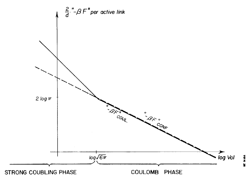
In going to weaker couplings, the fact that the values of the inverse squared couplings $\beta_{i}$ for which Bianchi identities become important coincides with the onset of the Coulomb phase should $a\;priori$ probably be regarded as a chance artifact of the lowest order approximation. However, we suspect that the transition to the Coulomb (organised) phase may be fundamentally related to having couplings weak enough to allow the self-organising effects of Bianchi identity constraints to be enforced in which case the coincidence may not be just a chance occurrence. In either event, the fact that $``-\beta F"_{per\;active\;link,\;conf.}$ is parallel to $``-\beta F"_{per\;active\;link,\;Coul.}$ for $\beta$ values exceeding that for which Bianchi identity corrections set in precludes an intersection of $``-\beta F"_{per\;active\;link,\;conf.}$ and $``-\beta F"_{per\;active\;link,\;Coul.}$ in this region of $\beta$ values. Therefore ignoring Bianchi identity corrections is justified when the $\beta_{crit.}$ are determined by the phase transition in the lowest order MFA.

For $\beta$ values corresponding to confinement,it is justifiable to neglect Bianchi identity corrections in the lowest order calculation of $\langle\exp S_{action,\;conf.}\rangle_{S_{ansa}}$ as the corrections first become relevant at the $\beta_{i,\;crit.}$ - i.e., upon leaving the confinement phase when the critical points are determined as the points of intersection for $``-\beta F"_{per\;active\;link,\;conf.}$ and $``-\beta F"_{per\;active\;link,\;Coul.}$.

Collecting the various factors in the expression (157) for $Z_{MFA}$ that have been calculated yields

$$Z_{MFA}=\exp(\langle S_{action,\;Coul.}-S_{ansa}\rangle_{S_{action,\;conf.}+S_{ansa}})\langle\exp(S_{action,\;conf.})\rangle_{S_{ansa}}\cdot Z_{S_{ansa}}$$

$$Z=\exp(``-\beta F")\geq Z_{MFA}\approx\exp(-\sum_{\Box}(\sum_{i\in``Coul."}d_{i}\cdot\frac{3}{2\tilde{\alpha}_{i}})+\sum_{\mbox{\begin{picture}(4.15,10.0)\put(0.0,3.0){\circle*{2.0}} \put(0.0,2.75){\line(1,0){7.0}} \put(7.3,3.0){\circle*{2.0}}\mbox{ } \end{picture} }}(\sum_{i\in``Coul."}d_{i}\cdot\frac{1}{2}))\cdot$$ (172)

$$\cdot\prod_{\Box}\prod_{j\in``conf."}\frac{(\pi)^{d_{j}/2}}{Vol(H)}\cdot\prod_{\mbox{\begin{picture}(4.15,10.0)\put(0.0,3.0){\circle*{2.0}} \put(0.0,2.75){\line(1,0){7.0}} \put(7.3,3.0){\circle*{2.0}}\mbox{ } \end{picture} }}\frac{1}{Vol(G/H)}\prod_{i\in``Coul."}(\frac{\pi}{\tilde{\alpha}_{i}})^{d_{i}/2}.$$

that is,

$$``-\beta F"=\log Z\geq-\sum_{\Box}\sum_{i\in``Coul."}d_{i}\frac{3}{2\tilde{\alpha}_{i}}+\sum_{-}\sum_{i\in``Coul."}\frac{d_{i}}{2}+\sum_{\Box}\log\frac{\prod_{j\in``conf"}(\pi)^{d_{j}/2}}{Vol(H)}+$$ (173)

$$+\sum_{-}\log(\frac{1}{Vol(G/H)}\prod_{i\in``Coul."}(\frac{\pi}{\tilde{\alpha}_{i}})^{d_{i}/2})$$

As we want to calculate a $``-\beta F"$ density rather than $``-\beta F"$ for the entire lattice ($``-\beta F"$ for an infinite lattice would of course be divergent), we now choose to work with the quantity $``-\beta F"=\log Z$ per active link. For a 4-dimensional hyper-cubic lattice, there are 3 active links per site (i.e., the number of dimensions reduced by the one dimension along which the gauge is fixed) and 6 plaquettes per site. This yields 2 plaquettes per active link. The expression for the total lattice $``\beta F"$ can now be rewritten as a “free energy density per active link”:

$$\log Z_{per\;active\;link}=``-\beta F\mbox{''}_{per\;active\;link}\geq$$ (174)

$$-2\sum_{i\in``Coul."}d_{i}\frac{3}{2\tilde{\alpha}_{i}}+\sum_{i\in``Coul."}\frac{d_{i}}{2}+2\log\left(\prod_{j\in``conf."}\frac{\pi^{d_{i}/2}}{Vol(H)}\right)+$$ (175)

$$+\log\left(\frac{1}{Vol(G/H)}\prod_{i\in``Coul."}(\frac{\pi}{\tilde{\alpha}_{i}})^{d_{i}/2}\right).$$

The extremum for $``-\beta F\mbox{''}_{per\;active\;link}$ w. r. t. the $\tilde{\alpha}_{i}$ is found for

$$\tilde{\alpha}_{i}=6\;\;\;(\forall i\in\mbox{``Coul."})$$ (176)

Inserting $\tilde{\alpha}_{i}=6$ in (175) yields $``-\beta F\mbox{''}_{per\;active\;link}$ to the approximation used here:

$$``-\beta F\mbox{''}_{per\;active\;link}=\sum_{i\in``Coul."}(-2d_{i}\frac{3}{2\cdot 6}+\frac{d_{i}}{2}+\log((\frac{\pi}{6})^{d_{i}/2})))+$$ (177)

$$+2\log\left(\frac{(\pi)^{\frac{\sum_{j\in``conf."}d_{j}}{2}}}{Vol(H)}\right)+\log(\frac{1}{Vol(G/H)})$$

$$=\log[\frac{(\pi/6)^{(dim(G/H))/2}}{Vol(G/H)}]+2\log[\frac{(\pi)^{(dim(H))/2}}{Vol(H)}]$$ (178)

6.4.1 The phase diagram for $SMG$ in lowest order $MFA$

The expression (178) for $``-\beta F_{per\;active\;link}$” provides a means of constructing an approximate phase diagram depicting the phase boundaries separating the partially confining phases of a non-simple gauge group. Using the weak coupling approximation, the goal in this section is the construction of a phase diagram for the $SMG$ using an action parameter space spanned by the logarithm of the volumes of the three different “basic” invariant subgroups $H_{i}$ where $\{i\}=\{U(1),\;SU(2),\;SU(3)\}$ (Figure17). In the absorbed notation, increasing values along the $i$th axis of this space correspond to increasing values of the “scaling” factor $\beta_{i}^{dim(H_{i})/2}$. Recall from Eqn. (124) that the relationship between volumes with and without the $\beta$’s absorbed into the metric is $Vol(H_{i})=\beta_{i}^{(dim(H_{i}))/2}\;vol(H_{i})$ where “$Vol$” and “$vol$” designate respectively volumes in terms of the metric with and without the $\beta_{i}$’s absorbed. In the “$Vol$”

At the boundary between a partially confining phase that confines along an invariant subgroup $H_{I}$ and another partially confining phase that is in confinement along an invariant subgroup $H_{J}$, the condition to be fulfilled for the critical volumes of the subgroups is obtained by equating the “free energy”, $``-\beta F$”, for these two phases. This leads to the condition

$$\log(6\pi)^{\frac{dim(H_{J})-dim(H_{I})}{2}}=\log\frac{Vol(H_{J})}{Vol(H_{I})}.$$ (179)

Uppercase indices $I,\;J,\cdots$ label the invariant subgroups corresponding to the eight possible partially confining phases of the $SMG$ obtainable when the discrete subgroups are not included among the basic invariant subgroups (i.e., using just the basic invariant subgroups $H_{i}$ with $i\in\{U(1),\;SU(2),\;SU(3)\}$). Of course the invariant subgroups $H_{J}$ do not in all cases coincide with one of the three “basic” invariant subgroups, but each $H_{J}$ is spanned by some subset of the basic invariant subgroups $H_{i}$ (having perhaps a discrete subgroup of the centre identified with the group identity).

The quantities “$Vol$” corresponding to the first eight invariant subgroups in the list (119) w.r.t. which there can be confinement in the approximation being considered in this Section are listed in the first column of Table 1. The second column contains the corresponding “$Vol$” quantities for the Coulomb-like factor group degrees of freedom.

Table 1: The first entry in a row is the quantity “$Vol$” for an invariant subgroup $H$ w.r.t which there can be confinement. The second entry in a row is the quantity “$Vol$”for the corresponding factor group $G/H$ degrees of freedom that behave in a Coulomb-like fashion.

$$\begin{array}[]{ll}Vol(\{1\})=1&Vol(SMG)=Vol(SMG/\{1\})=Vol(U(1)_{large})Vol(SU(2))Vol(SU(3))/6\\ Vol(U(1)(large))=Vol(U(1)_{large})&Vol(SMG/U(1))=Vol(So(3)\times SU(3)/Z_{3})=Vol(SU(2))Vol(SU(3))/6\\ Vol(SU(2))=Vol(SU(2))&Vol(SMG/SU(2))=Vol(U(3)_{factorgr.})=Vol(U(1)_{large})Vol(SU(3))/6\\ Vol(SU(3))=Vol(SU(3))&Vol(SMG/SU(3))=Vol(U(2)_{factor\;gr.})Vol(U(1)_{large})/6\\ Vol(U(2)_{subgroup})=Vol(U(1)_{large})Vol(SU(2))/2&Vol(SMG/U(2))=Vol({SU(3)/Z_{3}}_{factorgr.})=Vol(SU(3))/3\\ Vol(U(3)_{subgroup})=Vol(U(1)_{large})Vol(SU(3))/3&Vol(SMG/U(3))=Vol(So(3)_{factorgr.})=Vol(SU(2))/2\\ Vol(SU(2)\times SU(3)_{subgroup})=Vol(SU(2))Vol(SU(3))&Vol(SMG/(SU(2)\times SU(3)))=Vol(U(1)_{small})=Vol(U(1)_{large})/6\\ Vol(SMG)=Vol(U(1)_{large})Vol(SU(2))Vol(SU(3))/6&Vol(SMG/SMG)=Vol(\{1\})=1\\ \end{array}.$$ (180)

In particular, setting one of the invariant subgroups ($H_{I}$ for example) in Eqn. (179) equal to the group identity 1 yields the value of the volume of the subgroup $H_{J}$ at the interface with the totally Coulomb phase. That is, $\log Vol(H_{J})_{subgr.}=\log((6\pi)^{(dim(H_{J}))/2})$ at the boundary between the totally Coulomb phase and the partially confining phase with confinement along $H_{J}$. Within this partially confining phase, $\log Vol(H_{J})_{subgr.}\leq\log((6\pi)^{(dim(H_{J}))/2})$.

Alternatively, setting one of the invariant subgroups ($H_{J}$ for example) in (179) equal to the entire gauge group $G$ yields the value of the volume for the invariant factor group $G/H_{I}$ at the interface with the totally confining phase. That is $\log Vol(G/H_{I})_{factor\;gr.}=\log(6\pi)^{(dim(G/H_{I}))/2}$ at the boundary between the totally confining phase and the partially confining phase that is Coulomb-like w.r.t. $(G/H_{I})_{factorgr.}$. Within this partially confining phase, $\log Vol(G/H_{I})_{factorgr.}\geq\log(6\pi)^{(dim(G/H_{J}))/2}$.

In general (but not considering Higgsed degrees of freedom), each partially confining phase can be characterised by the invariant subgroup $H_{J}$ along which the corresponding degrees of freedom are confined or the factor group $G/H_{J}$ the cosets of which constitute the Coulomb-like degrees of freedom. Denoting by $L_{H_{J}}$ and $L_{G/H_{J}}$ the Lie algebras of respectively the invariant subgroup $H_{J}$ and the factor group $G/H_{J}$, we have of course that these Lie algebras span the gauge group Lie algebra $L_{G}$: $L_{G}=L_{H_{J}}\oplus L_{G/H_{J}}$.

To understand the approximate phase diagram of the $SMG$ sought here, it is useful to have as a reference the parallel study of the simpler Lie algebra-identical Cartesian product group $U(1)\times SU(2)\times SU(3)$. As stated previously, the group that we use as the Standard Model Group ($SMG$) is consistently taken to be

$$SMG=U(1)\times SU(2)\times SU(3)/``\mbox{\bf{Z}}_{6}"$$ (181)

where

$$``\mbox{\bf{Z}}_{6}"\stackrel{{\scriptstyle def}}{{=}}\{(2\pi,-{\mbox{\bf{1}}}^{(2\times 2)},\exp(i2\pi/3){\mbox{\bf{1}}}^{(3\times 3)})^{p}\mid p\in{\bf Z}\}.$$ (182)

This group has of course the same Lie algebra as the Cartesian product group $U(1)\times SU(2)\times SU(3)$ but has quite another global structure - namely that resulting when the subgroup of centre elements generated by the element $(2\pi,\;-{\mbox{\bf{1}}}^{(2\times 2)},\;\exp(i2\pi/3){\mbox{\bf{1}}}^{(3\times 3)})$ are identified with the group identity. In other words, the elements of the Standard Model Group ($SMG$) are, in this work, the set of cosets $g\cdot(2\pi,\;-{\mbox{\bf{1}}}^{(2\times 2)},\;\exp(i2\pi/3){\mbox{\bf{1}}}^{(3\times 3)})^{p}$ where $g\in U(1)\times SU(2)\times SU(3)$ and $p\in Z$. Each such coset consists of 6 elements of the group $U(1)\times SU(2)\times SU(3)$.

A characteristic feature of the phase diagram for the $SMG$ is that there is an extended phase boundary separating the totally confining and the totally Coulomb-like phases in the action parameter space spanned by just the three variables $\log Vol(H_{i})$ ($i\in\{U(1),\;SU(2),\;SU(3)\}$). This feature, which makes it impossible for all of the 8 possible partially confining phases to convene at a multiple point, is not present in the phase diagram for the Cartesian product group $U(1)\times SU(2)\times SU(3)$ where in fact the boundary separating the totally confining phase from the totally Coulomb-like phase is just one point in the 3-dimensional phase space where the 8 partially confining phases come together.

This difference in the phase diagrams for $SMG$ and $U(1)\times SU(3)\times SU(3)$ stems from the different way in which the volume of an invariant subgroup and the Lie algebra-identical factor group are related to each other and to the volume of the whole gauge group.

Generally, the volume of a confining subgroup $Vol(H_{J})$ and the volume of the factor group with the same Lie algebra are simply related. For a Cartesian product group $G=H_{1}\times H_{2}\times\cdots\times H_{J}\times\cdots$, the relation between the volume of a subgroup factor $H_{J}$ and the volume of the factor group with the same Lie algebra is particularly simple:

$$Vol(H_{J})=Vol(G/{\textstyle\prod_{{}_{cart.\;prod.,\;I\not=J}}}\cdots\times H_{I}\cdots)$$

where $G/{\textstyle\prod_{{}_{cart.\;prod.,\;I\not=J}}}\cdots\times H_{I}\cdots$

is the factor group having the same Lie algebra as the subgroup $H_{J}$. Characteristic for a Cartesian product group is that the centre is “disjoint” in the sense that the centre of a Cartesian product group is multiplicative in the centres of the subgroup factors. The centres of $SU(N)$ subgroups and $U(1)$ are isomorphic to respectively $\mbox{\bf{Z}}_{N}$ (cyclic group of order $N$) and $S_{1}$ (a circle).

The situation is a little more complicated when various subgroups of the centre of the Cartesian product group are identified with the identity element of the group (as is the case for $SMG$). In the case of $SMG$ 181, which is obtained from the Cartesian product group $U(1)\times SU(2)\times SU(3)$ by identifying the discrete “$\mbox{\bf{Z}}_{6}$” subgroup 182 of centre elements with the unit element (181), the volume is smaller by a factor 6 (the number of centre elements identified with the group identity) than that for the Cartesian product group $U(1)\times SU(2)\times SU(3)$. The greater complexity of the phase diagram for the $SMG$ arises because of the different ways that the total volume reduction factor “6” can be shared between (confined) invariant subgroups and corresponding (Coulomb-like) factor groups.

The group $U(N)=(U(1)\times SU(N))/``Z_{N}"$ as illustrative analogy to $SMG=(U(1)\times SU(2)\times SU(3))/``Z_{6}"$

In order to see how we get the phase diagram for the $SMG$ in the approximation considered here, it is useful to see how the distinctive difference in the phase diagrams for the gauge group $SMG=S(U(2)\times U(3))$ of Eqn. (181) and the Lie algebra-identical Cartesian product gauge group $U(1)\times SU(2)\times SU(3)$ comes about. To this end, it is enlightening (because it is easier) to consider the essentially analogous pair of groups $U(N)$ and the Cartesian product group $U(1)\times SU(N)$ (which of course has the same Lie algebra as $U(N)$). The relation of the group $U(N)$ to the Cartesian product group $U(1)\times SU(N)$ is analogous to the relation of the $SMG$ (Eqn. (181)) to the Cartesian product group $U(1)\times SU(2)\times SU(3)$ because $U(N)$, like the $SMG$, is obtained by identifying a discrete subgroup of the centre of the Cartesian product group with the group identity:

$$U(N)=(U(1)\times SU(N))/``\mbox{\bf{Z}}_{N}"$$ (183)

where

$$``\mbox{\bf{Z}}_{N}"\stackrel{{\scriptstyle def}}{{=}}\{(2\pi,\exp(i2\pi/N){\mbox{\bf{1}}}^{(N\times N)})^{p}\}\;\;\;(p\in\mbox{\bf{Z}}).$$ (184)

For both $U(N)$ and $U(1)\times SU(N)$, the choices for confining subgroups are the four invariant subgroups $SU(N)$, $U(1)$, $G$ (i.e., the whole group $U(N)$ or $U(1)\times SU(N)$) and 1 (the group identity). The Lie algebra-identical factor groups, listed in the same order, are $G/U(1)$, $G/SU(N)$, $G/\mbox{\bf{1}}$, and $G/G$. The invariant $(subgroup,\;\;factor\;\;group)$ pairs characterising (in a redundant way) the four partially confining phases are $(U(1)_{subgroup},(G/U(1))_{factor\;gr.})$, $(SU(N)_{subgroup},(G/SU(N))_{factor\;gr.})$, $(G_{subgroup},(G/G)_{factor\;gr.})$, $(\mbox{\bf{1}}_{subgroup},(G/\mbox{\bf{1}})_{factor\;gr.})$.

The last two $(subgroup,\;\;factor\;\;group)$ pairs designate the two special cases of partially confining phases in which all (physical) Yang-Mills degrees of freedom are respectively confining and Coulomb-like. The two remaining $(subgroup,\;\;factor\;\;group)$ pairs correspond to phases for which some of the (physical) Yang-Mills degrees of freedom are in confinement while others are in the Coulomb phase. For example, $(U(1)_{subgroup},(G/U(1))_{factor\;gr.})$ designates the partially confining phase with confining degrees of freedom along $U(1)$ and degrees of freedom that are Coulomb-like w.r.t. the factor group $G/U(1)$.

The phase diagram for $U(N)$ is different from that for the Cartesian product group $U(1)\times SU(N)$: the phase in which the $U(1)$ degrees of freedom are confining and the $SU(N)$ degrees of freedom are Coulomb-like and the phase in which the roles of $U(1)$ and $SU(N)$ are exchanged have phase boundaries that do not have any points in common in the action parameter space (phase diagram) considered (Figure 15). Rather there is an extended boundary between the totally Coulomb and the totally confining phases in contrast to the phase diagram for $U(1)\times SU(2)$ where the boundary between the totally Coulomb-like and totally confinement-like phases is just a point (the multiple point) at which the other partially confining phases also convene.

For the Cartesian product group $U(1)\times SU(N)$, subgroups and corresponding (i.e., Lie algebra-identical) factor groups have equal volumes. In the metric in which the $\beta$’s are not absorbed into the metric tensor, this means simply that $vol(U(1))_{subgr.}=vol((U(1)\times SU(N))/SU(N))_{factor\;gr.}$ and $vol(SU(N))_{subgr.}=vol((U(1)\times SU(N))/U(1))$ where we continue to use the notation in which “$vol$” with lower case “$v$” designates group volumes without absorbed $\beta$’s. For $U(1)\times SU(N)$ the equality $\log Vol(U(1))_{subgr.}=\log Vol((U(1)\times SU(N))/SU(N))_{factorgr.}$ is fulfilled for the same value of the absorbed quantity $(\beta_{1})^{\frac{1}{2}}$ on the right and left sides of the equation. The same applies for the absorbed quantity $(\beta)^{\frac{N^{2}-1}{2}}_{N}$ in the equality $\log Vol(SU(N))_{subgr.}=\log Vol((U(1)\times SU(N))/U(1))_{fac.gr.}$. Therefore, the phase boundaries separating the confinement and Coulomb phases - for either the $U(1)$ or the $SU(N)$ gauge degrees of freedom - coincide and the phase diagram consists of the two straight lines

$$\log Vol(U(1))=\log(6\pi^{(dim(U(1)))/2})=\log\sqrt{6\pi}$$

and

$$logVol(SU(N))=\log(6\pi^{(dim(SU(N)))/2}).$$

that intersect at the multiple point where all 4 partially confining phases convene. (see Figure 14).

Figure 14: Phase diagram for the Cartesian product group $U(1)\times SU(N)$.

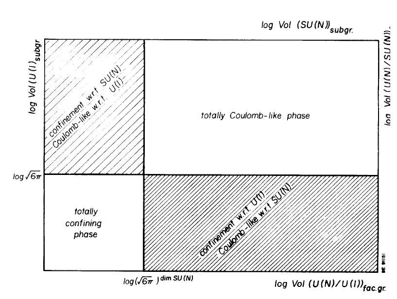
The Phase Diagram for the Group $U(N)$

For $U(N)$ this is not the case: rather $vol(U(1))_{subgr.}=N\cdot vol(U(N)/SU(N))_{factor\;gr.}$ and $vol(SU(N))_{subgr.}=N\cdot vol(U(N)/U(1))_{factor\;gr.}$. The reason is that the identification (with the group identity) of a $N$-element discrete subset common to the centre of the subgroups $U(1)$ and $SU(N)$ reduces the volume of $U(N)$ relative the Lie algebra-identical Cartesian product group $U(1)\times SU(N)$ by a factor equal to the $N$ centre elements identified with the identity in obtaining $U(N)$ from $U(1)\times SU(N)$. That is,

$$VolU(N)=\frac{Vol(U(1)\times SU(N))}{N}=\frac{VolU(1)_{subgr.}Vol(SU(N))_{subgr.}}{N}.$$ (185)

But it is also true that

$$Vol(U(N))=VolU(1)_{subgr.}Vol(U(N)/U(1))_{fac.\;gr.}$$ (186)

$$=VolSU(N)_{subgr.}Vol(U(N)/SU(N))_{fac.\;gr.}.$$

From Eqn. (185) and Eqn. (186) it can be concluded that for $U(N)$ one has

$$Vol(U(N)/SU(N))_{fac.\;gr.}=\frac{VolU(1)_{subgr.}}{N}$$ (187)

and

$$Vol(U(N)/U(1))_{fac.\;gr.}=\frac{VolSU(N)_{subgr.}}{N}$$ (188)

i.e., in going from $U(1)\times SU(N)$ to $U(N)$, the volume of a factor group with a given sub-Lie algebra is reduced by a factor $N$ relative to the subgroup with this sub-Lie algebra. This happens because the subgroup corresponding to any given sub-Lie algebra has the same volume in $U(N)$ as in $U(1)\times SU(N)$, so it is the factor group that bears the entire $1/N$ group volume reduction factor.

Inasmuch as critical values for the inverse squared couplings (i.e., the $\beta_{i}$’s) must ultimately be extracted from the volume expressed in the metric into which the $\beta_{i}$’s are absorbed (Eqn. (124)), it is important to realize that a given $\beta_{i}$ can be absorbed into: (1) a subgroup volume or (2) a factor group volume. This is true for $U(N)$ as well as the $SMG$:

1. Consider a subgroup $H_{J}$ that coincides with a the $i$th basic invariant subgroup $H_{i}$ or a Cartesian product of basic invariant subgroups that includes $H_{i}$. In these cases, $\beta_{i}$ is absorbed into the quantity $Vol(H_{J})$ that, in directions within the $i$th basic Lie sub-algebra, is calculated using in the metric induced by the group along the invariant subgroup $H_{i}$. Distances within this subgroup are proportional to $\sqrt{\beta_{i}}$. This essentially means that distances along $H_{i}$ are measured in units of the root mean square extent of quantum fluctuations.

   For the partially confining phase confined along the Cartesian product of say the $i$th and $j$th basic invariant subgroups: $H_{J}=H_{i}\times H_{j}$, the interface with the totally Coulomb phase coincides with the critical value of $Vol(H_{J}$) as determined by Eqn. (179) when the invariant subgroup $H_{I}$ is set equal to the gauge group identity:

   $$(6\pi)^{(dim(H_{i})+dim(H_{j}))/2}=Vol(H_{i})Vol(H_{j})=$$ (189)

   $$=\beta^{dim(H_{i})/2}\beta^{\beta(H_{j})/2}vol(H_{i})vol(H_{j}).$$

   In the case of $U(N)$, taking $H_{I}=$1 in (179) and the other invariant subgroup $H_{J}$ to be $H_{J}=U(1)$ or $SU(N)$ leads to the equations

   $$(6\pi)^{(dim(U(1)))/2}=Vol_{crit}(U(1)_{subgr.})=\sqrt{\beta_{1\;crit}}vol(U(1)_{subgr})$$ (190)

   and

   $$(6\pi)^{(dim(SU(N)))/2}=Vol_{crit}(SU(N)_{subgr})=(\sqrt{\beta_{N\;crit}})^{(N^{2}-1)}vol(SU(N)_{subgr})$$ (191)

   at the interface of the totally Coulomb-like phase and the phases confined w.r.t. respectively $U(1)$ and $SU(N)$.

2. Another occurrence of $\beta_{i}$ is in the Volume expressed in the metric induced by the group along an invariant factor group the Lie subalgebra of which includes that of the $i$th basic invariant subgroup $H_{i}$. Assuming that the Lie algebra of the factor group coincides with that of the invariant subgroup $H_{I}$, we can write this factor group as $G/H_{J}$ $(J\neq I)$. where $G$ denotes the gauge group $U(N)$ or $SMG$ as appropriate to the context. By assumption we have $H_{i}\subseteq H_{I}$ (i.e., the Lie algebra of the factor group includes but does not necessarily coincide with the Lie sub-algebra of the i$th$ basic invariant subgroup). The Volume of the factor group is the Volume of the Lie sub-algebra-identical basic invariant subgroup divided by a natural number $n$:

   $$Vol(G/H_{J})=\frac{Vol(H_{I})}{n}$$ (192)

   This natural number $n$is the the total number of identified centre elements of the gauge group divided by the number of these same identified group elements that are identified in the invariant subgroup $H_{J}$ if the latter is not simply a basic invariant subgroup (or a Cartesian product of basic invariant subgroups). As an example, consider the factor group $SMG/U(2)$ having the same Lie algebra as $SU(3)$. For $Vol(SMG/U(2))$ (which contains an absorbed $\beta_{SU(3)}$, we have that $Vol(SMG/U(2))=Vol(SMG/((U(1)\times SU(2))/\mbox{\bf{Z}}_{2})=$ $Vol(SU(3)_{subgr}/(6\cdot\frac{1}{2})$. The “natural number” $n=6\cdot\frac{1}{2}=3$ arises as the number of centre elements of $U(1)\times SU(2)\times SU(3)$ that are identified in the $SMG$ (i.e., 6) divided by the the number of these that are already identified in $U(2)$ (i.e., 2). For the critical value of Vol($SMG/U(2)$), the absorbed quantity $\beta_{SU(3)}$ is a factor $(\frac{6}{2})^{2/dim(SU(3))}$ larger that the $\beta_{SU(3)}$ value absorbed in the critical value of Vol($SU(3)$).

   For the partially confining phase having a Coulomb-like distribution of the cosets $g\cdot H_{J}$ with $g\in G$ (or, equivalently, the partially confining phase that is confined along $H_{J}$)), the interface with the totally confined phase coincides with the critical value of $Vol(G/H_{J}$ as determined by Eqn. (179) upon setting one of the subgroups in this equation equal to the whole gauge group. Thinking of $G=U(N)$, this yields for the critical volume of the factor group with the Lie algebra of $U(1)$ (i.e., $U(N)/SU(N)$)

   $$(6\pi)^{(dim(U(N))-dim(SU(N)))/2}=(6\pi)^{dim(U(1))/2}=Vol((U(N)/SU(N))_{factor\;group})=$$ (193)

   $$=(\beta_{U(1)})_{fac\;gr}^{(dim(U(1))/2}\cdot vol((U(N)/SU(N))_{factor\;group})=(\beta_{U(1)})_{fac\;gr}^{(dim(U(1))/2}\cdot\frac{vol(U(1))}{N}.$$

   But we also have that (193) is the critical value of $Vol(U(1))=(\beta_{U(1)})^{\frac{dim(U(1))}{2}}_{subgr}vol(U(1))$. Using that $vol(U(1))=N\cdot vol(U(N)/SU(N))$, we see that the relation between the $\beta_{U(1)}$ absorbed into $Vol(U(1))$ and that absorbed into $Vol(U(N)/SU(N))$ is

   $$(\beta_{U(1)})_{fac\;gr}=N^{\frac{2}{dim(U(1))}}(\beta_{U(1)})_{sub\;gr}$$ (194)

   An analogous argument leads to the relation

   $$(\beta_{SU(N)})_{fac\;gr}=N^{\frac{2}{dim(SU(N))}}(\beta_{SU(N)})_{sub\;gr}$$ (195)

   The subscripts “$fac\;gr$” and “$subgr$” on $\beta$, put in above for clarity, are normally omitted inasmuch as these subscripts can be figured out from the context in which a $\beta$ appears.

   $$=Vol((U(N)/U(1))_{factor\;group})=(\beta_{N})^{(dim(SU(N))/2}vol((U(N)/U(1))_{factor\;group}).$$

In a coordinate system spanned by the variables $\log Vol(H_{i})$ ($H_{i}\in\{U(1),\;SU(N)\}$), the phase diagram for $U(N)$ is completely determined by locating two special points “1” and “2” of the phase diagram: denote by “1” a point in the partially confining phase that is Coulomb-like solely along $U(1)$ but which is very close to the corner where this phase is in contact with the totally Coulomb and totally confining phases; denote by “2” a point in the partially confining phase that is confined solely along $U(1)$ but which again is very close to the corner where this phase is in contact with the phases that are totally confining and totally Coulomb-like (see Figure 15).

Figure 15: Phase diagram for $U(N)$.

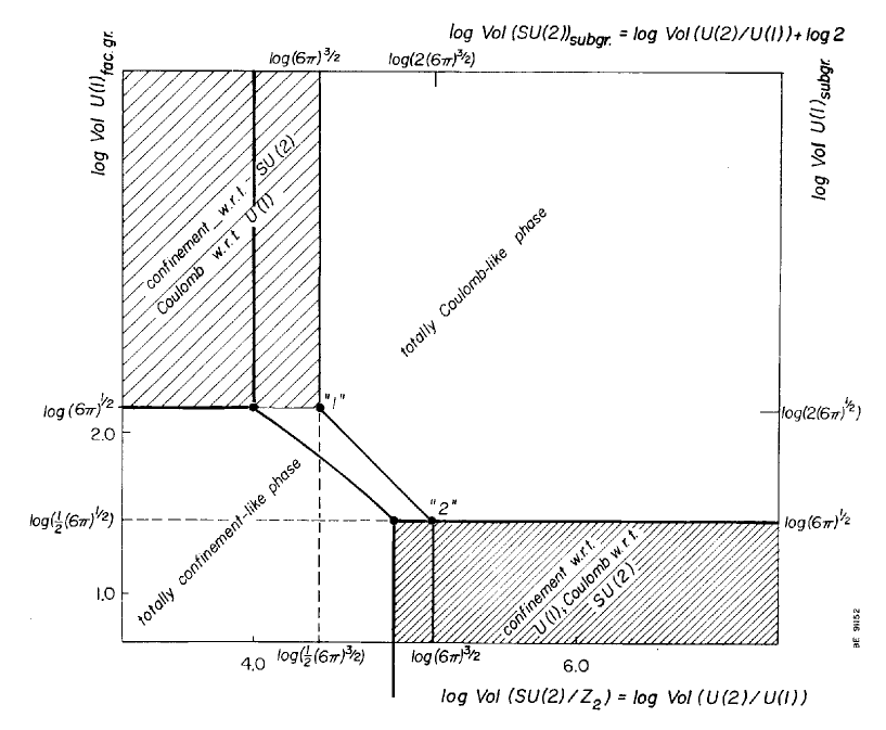
As has been pointed out, the centre of $U(N)$ contains a $\mbox{\bf{Z}}_{N}$ that is shared by both of the invariant subgroups $SU(N)$ and $U(1)$. Near “1” but in the phase with only $SU(N)$ confining, the (Coulomb-like)$U(1)$ degrees of freedom are realized as the cosets $g\cdot SU(N)\in U(N)/SU(N)$ ($g\in U(N)$). The picture one can have in mind is that the distribution of $U(1)$ degrees of freedom is tightly clustered about the coset $\mbox{\bf{1}}\cdot SU(N)$ whereas the confining $SU(N)$ degrees of freedom fluctuate (within the the cosets) somewhat more. Effectively, the large fluctuations along these cosets $G\cdot SU(N)$ make the elements within these cosets equivalent to the group identity as far as the $U(1)$ degrees of freedom are concerned. This applies also to the elements of the $\mbox{\bf{Z}}_{N}$ subgroup of the centre that is shared with the $U(1)$: at the point “1”, large fluctuations along $U(N)$ render the elements of the $Z_{N}\subset U(N)$ essentially equivalent to the identity. But this same $Z_{N}$ is shared with $U(1)$: $Z_{N}\subset U(1)$. Hence the Coulomb-like $U(1)$ degrees of freedom are realized on the manifold (consisting of the cosets $u\cdot\mbox{\bf{Z}}_{N}\in U(1)/\mbox{\bf{Z}}_{2}\simeq U(N)/SU(N)$) $(u\in U(1)$) having a volume that is reduced by a factor $\#\mbox{\bf{Z}}_{N}\stackrel{{\scriptstyle def}}{{=}}N$ relative to the volume of the manifold of the $U(1)$ subgroup.

Near the point “2” (but in the phase with confinement along $U(1)$) in the phase diagram for $U(N)$, the roles of $U(1)$ and $SU(N)$ are reversed: the larger fluctuations are within the cosets of the confinement-like $U(1)$ degrees of freedom and the Coulomb-like $SU(2)$ degrees of freedom are realized as the cosets $g\cdot U(1)\in SU(N)/\mbox{\bf{Z}}_{2}\simeq U(N)/U(1)$ $(g\in U(N))$.

The coordinates of corner “1” are

$$(\log Vol(SU(N))_{subgr.}),\log Vol((U(N)/SU(N))_{fac.\;gr.}))=(\log(\sqrt{6\pi})^{N^{2}-1},\log\sqrt{6\pi})$$ (196)

and the coordinates of corner “2” are

$$(\log Vol((U(N)/U(1))_{fac.\;gr.}),\log Vol((U(1))_{subgr.})=(\log(\sqrt{6\pi})^{N^{2}-1},\log\sqrt{6\pi}).$$ (197)

To plot the coordinates of the two corners “1” and “2” in a space spanned by axes corresponding to the variables $\log Vol(H_{i})$ $(i\in\{U(1),SU(N)\})$, we shall work with two sets of labels for each axis: one set for subgroups and another set for the Lie algebra identical factor group. These are simply related: the set of axis labels for factor groups is shifted relative to the axis labels for subgroups by an amount $\log N$ in the direction of increasing $\log Vol(H_{i})$. This simply reflects the fact that for a factor group, the quantity $Vol_{fac.\;gr.}$ attains the same numerical value as the quantity $Vol_{subgr.}$ for the Lie algebra-identical subgroup only after $\beta_{i}$ is “scaled up” by a factor $N^{2/d_{i}}$ (where $d_{i}=dim(H_{i})$ with $H_{i}\in\{U(1),SU(N)\})$.

To be in the partially confining phase of $U(N)$ that is Coulomb-like solely w.r.t. $U(1)$, one of the requirements is that $\log Vol((SU(N))_{subgr})\leq(6\pi)^{\frac{N^{2}-1}{2}}$. To be in the phase that is confining solely w.r.t. $U(1)$, one of the requirements is that $\log Vol((U(N)/U(1))_{fac\;gr})\geq(6\pi)^{\frac{N^{2}-1}{2}}$. But it has been seen that when $Vol(SU(N))=Vol(U(N)/U(1))$, the $\beta_{SU(N)}$ absorbed into $Vol(U(N)/U(1))$ is a factor $N^{2/dimSU(N)}$ larger than than the $\beta_{SU(N)}$ absorbed into $Vol(SU(N))$. So there is an interval of length $\log N$ extending from $\log Vol(SU(N))_{subgr.}=\log(6\pi)^{dim\;SU(N)/2}$ to $\log Vol(U(N)/U(1))_{factor\;gr.}=\log(6\pi)^{dimSU(N)/2}$ in which it is only possible to realize the totally confining or totally Coulomb-like phases of $U(N)$. The same is seen to be true for the interval of length $\log N$ extending from $\log Vol(U(1))_{subgr.}=\log(\sqrt{6\pi})$ to $\log Vol(U(N)/SU(N))_{factorgr.}=\log(\sqrt{6\pi})$.

The straight line connecting the points “1” and “2” in the phase diagram of Figure 15 is the phase interface separating the total confinement and total Coulomb phases of the theory. To see this, write the equation for this line:

$$\log Vol((U(N)/SU(N))_{fac.\;gr.})=\log\sqrt{6\pi}-(\log Vol(SU(N))_{subgr.}-\log((\sqrt{6\pi})^{N^{2}-1})).$$ (198)

Rearranging yields

$$\log(6\pi)^{N^{2}/2}=\log(Vol(SU(N))_{subgr.}Vol((U(N)/SU(N))_{fac.\;gr.})=\log VolU(N)$$ (199)

which from Eqn. (179) with $H_{I}=U(N)$ and $H_{J}={\mbox{\bf{1}}}$ is seen to be the condition to be satisfied at the interface separating the totally Coulomb and totally confining phases.

In other words, starting at the point “1” in Figure 15 (where $U(1)$ alone is Coulomb), the other end of the phase boundary separating the totally confining and the totally Coulomb-like phases (point “2” where alone $SU(N)$ is Coulomb in Figure 15) is attained by going $-\log N$ along the $\log Vol(U(1))$ axis and $+\log N$ along the $\log Vol(SU(N))$ axis.

Phase Diagram for the Standard Model Group

With the relationship between $U(1)\times SU(N)$ and $U(N)$ and the corresponding phase diagrams in mind, the slightly more complicated phase diagram for the $SMG$ can essentially be constructed by analogy insofar as the $SMG$ and $U(1)\times SU(2)\times SU(3)$ are related in a way much like the relation between $U(N)$ and $U(1)\times SU(N)$.

For the $SMG$, the corner of the partially confining $SMG$ phase where $U(1)$ alone is Coulomb (call it point “1” as it is the point analogous to point “1” in Figure 15) and the corner of the partially confining phase where alone $U(1)$ is confining (call it point “2” as it is the point analogous to point “2” in Figure 15) have coordinates in a 2-dimensional phase diagram spanned by $\log Vol((SU(2)\times SU(3))$ and $\log Vol(U(1))$ (containing the shaded planes of Figure 16) that are given by respectively

Figure 16: Construction of the phase diagram for the Standard Model Group to lowest order.

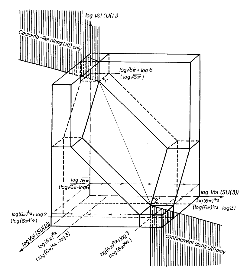
$$(\log Vol(SU(2)\times SU(3))_{subgr.},\log Vol(SMG/(SU(2)\times SU(3))_{factor\;gr.})=$$ (200)

$$(\log(\sqrt{6\pi})^{3+8}),\log(\sqrt{6\pi}))$$

at point “1” and

$$(\log Vol(SMG/U(1))_{factor\;gr.},\log Vol(U(1))_{subgr.})=$$ (201)

$$=(\log((\sqrt{6\pi})^{3+8}),\log(\sqrt{6\pi}))$$

at point “2”. The (somewhat redundant) subscripts $``subgr.$” and $``fac.\;gr.$” indicate explicitly which set of labels on a $\log Vol$ axis that the numbers on the right-hand side of the equalities refer to. Starting at point “1” in Figure 16, point “2” is reached by decreasing $\log Vol((SMG/(SU(2)\times SU(3)))_{factor\;gr.}$ by $\log 6$ and increasing $\log Vol_{crit.}((SU(2)\times SU(3))_{subgr.}$ by $\log 6$.

While point “1” and “2” are the termini of a line separating the total confinement and total Coulomb phase, this is not the complete story for the $SMG$. Recall that in the $U(N)$ phase diagram, all the elements of the $\mbox{\bf{Z}}_{N}$ of centre elements shared by $U(1)$ and $SU(N)$ are shared in such a way that, in going from “1” to “2” (or vice versa) there is a redistribution of fluctuations along the cosets of just two possible coset structures (recall that is this section possibility of having $\mbox{\bf{Z}}_{N}$ confined is ignored). At point “1” there are large fluctuations along the cosets $g\cdot SU(N)\in U(N)/SU(N)$ ($g\in U(N)$) while the coset-valued $U(1)$ degrees of freedom are rather tightly clustered about the coset $\mbox{\bf{1}}\cdot SU(N)$. At point “2”, fluctuations have become large along the cosets $g\cdot U(1)\in U(N)/U(1)$ $g\in U(N)$ while the Coulomb-like $SU(N)$ degrees of freedom are tightly clustered about the coset $\mbox{\bf{1}}\cdot U(1)$. For $U(N)$, there are only two sets of cosets; fluctuations are large along one or the other of these sets at the points “1” or “2”. The volume reduction factor $N=\#\mbox{\bf{Z}}_{N}$ for $U(N)$ relative to $U(1)\times SU(N)$ is bourn solely by the Coulomb-like $U(1)$ degrees of freedom at “1” and solely by the Coulomb-like $SU(N)$ degrees of freedom at “2”.

Unlike the case for $U(N)$, the $SMG$ has among the possible invariant subgroups two that have centre elements identified relative to the corresponding subgroups in $U(1)\times SU(2)\times SU(3)$: these are $U(2)\overline{\simeq}(U(1)\times SU(2))/\mbox{\bf{Z}}_{2}$ and $U(3)\stackrel{{\scriptstyle-}}{{\simeq}}(U(1)\times SU(3))/\mbox{\bf{Z}}_{3}$. We want now to think about going from “1” to “2” by way of “3” in the $SMG$ phase diagram. Now in our $SMG\stackrel{{\scriptstyle def}}{{=}}S(U(2)\times U(3))$ we know that the elements of “$\mbox{\bf{Z}}_{6}$” are identified (which means that they are rendered indistinguishable because of fluctuation patterns of one sort or another). Now at point “1”, the fluctuation pattern that causes the identification of the elements of $\mbox{\bf{Z}}_{6}$ is that of large fluctuations along $SU(2)$ and $SU(3)$. In going from point “1” towards point “3”, fluctuations along $SU(3)$ decrease and fluctuations along $U(1)$ increase until, at “3”, the $\mbox{\bf{Z}}_{3}\in``\mbox{\bf{Z}}_{6}"$ are identified due to fluctuations along $U(1)$ instead of fluctuations along $SU(3)$ while the increased fluctuations along $U(1)$ means that the $\mbox{\bf{Z}}_{2}\in``\mbox{\bf{Z}}_{6}"$ are now accessed by fluctuations both along $U(1)$ and $SU(2)$. But the group for which the elements of a $\mbox{\bf{Z}}_{2}$ can be accessed either by going along a $U(1)$ subgroup or a $SU(2)$ subgroup is just $U(2)$ which in fact coincides with the confined degrees of freedom at point “3” (see Figure 17). In going from point “3” to point “2”, fluctuations along $U(1)$ increase even more while now fluctuations along $SU(2)$ decrease (and fluctuations along $SU(3)$ remain small). Upon reaching point “2”, all elements of “$\mbox{\bf{Z}}_{6}$” are accessed exclusively by fluctuations along $U(1)$ corresponding to $U(1)$ alone confining at point “2”.

Figure 17: The lowest order phase diagram for the $SMG$ showing the 8 partially confining phases and the “diamond” interface separating the totally confining and totally Coulomb-like phase.

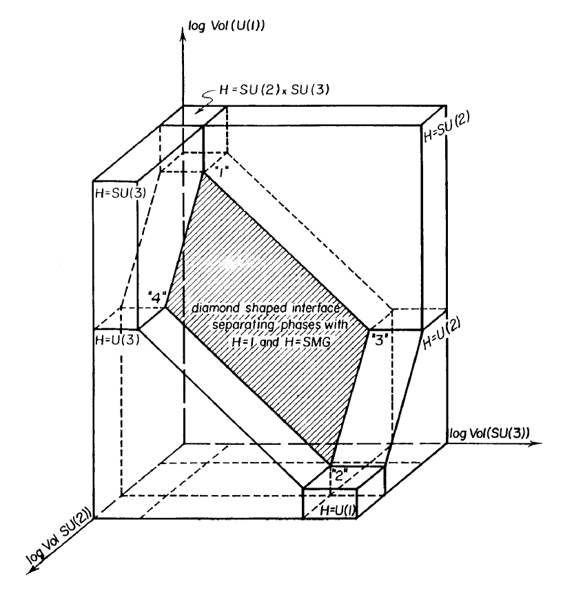
Having $U(2)$ and $U(3)$ allows the volume factor of six bourn by the $U(1)$ Coulomb-like degrees of freedom at “1” to be redistributed to Coulomb-like $SU(2)$ and $SU(3)$ degrees of freedom at respectively corner “3” and “4” (see Figure 17). At the intermediate point “3” en route from “1” to “2”, the volume reduction factor bourn by the $U(1)$ degrees of freedom is reduced from six at “1” to three at “3”; at point “3” the remaining fac two of the total volume reduction factor of six is bourn by the $U(2)=(U(1)\times SU(N))/\mbox{\bf{Z}}_{N}$ subgroup of confined degrees of freedom. An analogous scenario involves a point “4” in Figure 17 where the Coulomb-like $U(1)$ degrees of freedom bear a volume reduction factor of 2 while the remaining factor of 3 is bourn by the confining $U(3)$ degrees of freedom.

In the $MFA$ weak coupling approximation, having $U(2)$ and $U(3)$ as invariant subgroups in the $SMG$ has the effect of changing the phase boundary line separating the total confinement and total Coulomb phases into a phase boundary plane in the space spanned by the $\log Vol_{i}$. Here $i$ is any one of the three “basic” invariant subsets of the $SMG$. The reason as suggested above is that the presence of the $U(2)$ and $U(3)$ subgroups allows two alternatives to the straight line route connecting the corner of the partially confining phase with $U(1)$ alone Coulomb with the corner of the partially confining phase with $U(1)$ alone in confinement. These two alternative routes define the boundaries of the $SMG$ phase boundary plane separating the total confinement and total Coulomb phases. Starting at point “1” in Figure 16, one alternative route to point “2” is that for which $\log Vol(SU(2)_{subgr.})$ is held at the constant value $(\sqrt{6\pi})^{3}$ until point “3” is reached by decreasing respectively increasing the $\log Vol((SMG/(SU(2)\times SU(3))_{factor\;gr.})$ and $\log Vol(SU(3)_{subgr.})$ coordinates of point “1” by the amount $\log 3$. At point “3”, $\log Vol((SMG/U(2))_{factor\;gr.})$ is held at the constant value $(\sqrt{6\pi})^{8}+\log 3$ while decreasing respectively increasing the coordinates $\log Vol((SMG/(SU(2)\times SU(3)))_{factor\;gr.})-\log 3$ and $\log Vol(SU(2)_{subgr.})$ by the amount $\log 2$. This brings us to point “2”. Exchanging the roles of $SU(2)$ and $SU(3)$ yields the second alternative route to point “2” via point “4” . These two alternative routes via point “3” and point “4” define the boundaries of the diamond-shaped interface separating the total confinement and total Coulomb phases as shown in Figure 16.

6.4.2 Next order in perturbation

The weak coupling approximation used above is really the approximation in which the fluctuations around the unit element are so small that one can approximate the group by the Lie algebra (the tangent plane approximation). For the invariant subgroup(s) in the confining phase, the calculations above utilise only that the fluctuation of the plaquette variable is small enough for the validity of this approximation whereas it is used for both the link and the plaquette variables for the Coulomb phase degrees of freedom. For the same values of the $\beta_{i}$ ’s, the fluctuations are larger for the confinement phase than for the Coulomb phase. Therefore it is to be anticipated that the numerically most important correction will come from the next order correction estimate for the confining degrees of freedom.

Next order corrections come about by using a corrected Haar measure that reflects the curvature of the group manifold and a corrected rule of composition of Lie algebra vectors for non-Abelian groups when group multiplication is referred to the Lie algebra. In the tangent space approximation for the group manifolds with curvature that were used in calculations to leading order, the rule of composition is approximated by simple vector addition of Lie algebra elements. This approximation neglects the non-commutativity of the non-Abelian group generators.

When both corrections - i.e., the correction for the Haar measure and the correction for non-commutativity - are included, the defining condition for the phase boundary separating the totally Coulomb and totally confined phases becomes

$$\log Vol(SMG)=\log(6\pi)^{6}-\underbrace{\frac{1}{2\beta_{2}}-\frac{2}{\beta_{3}}}_{\mbox{Haar measure}}+\underbrace{\frac{1}{24\beta_{2}}+\frac{1}{6\beta_{3}}}_{\mbox{non-commutativity}}$$ (202)

The leading order terms of this equation, i.e., $Vol(SMG)=\log(6\pi)^{6}$ are identical with the condition (179) in the special case where $H_{J}=SMG$ and $H_{I}=\mbox{\bf{1}}$. The details of these next to lowest order corrections are dealt with in Appendices 11.1, 11.2 and 11.3.

6.5 Using discrete subgroups of the centre to get a multiple point

In the $SMG$ phase diagram of Figure 17, it is seen that the 8 partially confining phases that can be realized in a parameter space spanned by parameters proportional to $\beta_{1}$, $\beta_{2}$, and $\beta_{3}$ do not convene at a multiple point/surface. When the set of constituent invariant subgroups is restricted to the set $\{SU(3),SU(2),U(1)\}$, the factorisation property (139) cannot be realized for all of the first 8 invariant subgroups of (119).

This factorisation property can be realized for all the 13 invariant subgroups $H\lhd SMG$ (or all the 5 invariant subgroups $H\lhd U(N)$) using the previously defined set of constituent invariant subgroups. That is, it is possible to factorise $Vol(H)$ into a product of some subset of a common set of 5 factors $(1/p_{i})Vol(K_{i})$ (with $p_{i}\in N^{+}$) (3 such factors for $U(N)$) corresponding to the constituent invariant subgroups $K_{i}\in\{\mbox{\bf{Z}}_{2},\mbox{\bf{Z}}_{3},U(1),SU(2),SU(3)\}$ for the $SMG$ (for $U(N)$, the constituent invariant subgroups are $K_{i}\in\{SU(N),U(1),\mbox{\bf{Z}}_{N}\}$). Then it is possible by adjustment of the parameters $\beta_{1},\beta_{2},\beta_{3},\xi_{2},\xi_{3}$ to make the quantities $\log Z_{H\;per\;active\;link}$ equal for each invariant subgroup $H\lhd SMG$ (the same applies to each invariant subgroup $H\lhd U(N)$ using the parameters $\beta_{1},\beta_{N},\xi_{N}$). This is equivalent to finding a non-generic multiple point (because $5<n_{SMG}-1=13-1$ for the $SMG$ and $3<n_{U(N)}-1=5-1$ for $U(N)$).

We explicitly demonstrate the factorisability of $Vol(H)$ in the sense that we show that it is of the form $Vol(H)=\mbox{product of some factors}(1/p_{i})Vol(K_{i})$ for each invariant subgroup $H$ of both $SMG$ and $U(N)$. To do this, we use a calculational trick in which we replace each $H$ by a Cartesian product group related to $H$ by a homomorphism that is locally bijective. This (to $H$) locally isomorphic Cartesian product group consists of the covering Lie (sub)groups corresponding to the gauge degrees of freedom that the invariant subgroup $H$ involves supplemented by the discrete constituent invariant subgroups contained in these Lie subgroups. For all the invariant subgroups $H$, the Cartesian product group replacement can be obtained by simply omitting factors in the Cartesian product group replacement $\mbox{\bf{Z}}_{2}\times\mbox{\bf{Z}}_{3}\times U(1)\times SU(2)\times SU(3)$ for the whole $SMG$. Of course such a Cartesian product group in general differs in global structure from the invariant subgroup $H$ that it replaces. However, as we are only interested in the quantity $Vol(H)$ for invariant subgroups $H$, we can use a correction factor $1/p_{{}_{H}}$ to adjust the quantity $Vol$ of the Cartesian product group replacement for $H$ so as to make it equal to $Vol(H)$.

As an example, consider the invariant subgroup $H=U(2)\subset SMG$ which is locally isomorphic to the Cartesian product group $U(1)\times SU(2)\times\mbox{\bf{Z}}_{2}\times\mbox{\bf{Z}}_{3}$. By this we mean that, assuming the modified Manton action (133) and a weak coupling approximation, the Cartesian product group $U(1)\times SU(2)\times\mbox{\bf{Z}}_{2}\times\mbox{\bf{Z}}_{3}$ simulates the subgroup $U(2)\subset SMG$ in the sense that the regions on the group manifold of $U(2)\subset SMG$ in which the probability distribution $e^{S_{\Box}}$ is concentrated can be brought into a one to one correspondence with centres of fluctuation sharply peaked around points in the Cartesian product group. In other words, for $U(2)\subset SMG$, the region of correspondence with the Cartesian product group is the composite of 6 small neighbourhoods around the elements $p\in\mbox{span}\{\mbox{\bf{Z}}_{2},\mbox{\bf{Z}}_{3}\}$. Even though the Cartesian product group in this example contains $2\cdot 2\cdot 3$ elements for each element in $U(2)$, the action on the Cartesian product group is defined so as to be $-\infty$ everywhere except at one of the these 12 elements where this action then has the same value as the action at corresponding element of $U(2)$.

In order to make the quantity $Vol(U(1)\times SU(2)\times\mbox{\bf{Z}}_{2}\times\mbox{\bf{Z}}_{3})$ equal to $Vol(U(2))$ (for $U(2)\subset SMG$) , the former must be reduced by a factor $p_{U(2)}$ obtained as follows: Remember that the $U(1)$ embedded in the $SMG$ has a length $6\cdot 2\pi$ so that the $U(2)$ subgroup lying in the $SMG$ is $(U(1)_{12\pi}\times SU(2))/\mbox{\bf{Z}}_{2}$. Comparing the quantity $Vol(U(2))=Vol(U(1)_{12\pi})\cdot Vol(SU(2))/\mbox{\bf{Z}}_{2}$ and the quantity $Vol$ for the locally isomorphic Cartesian product group: $Vol(U(1)_{12\pi})\times Vol(SU(2))\times Vol(\mbox{\bf{Z}}_{2})\times Vol(\mbox{\bf{Z}}_{3}))$, it is seen that, relative to $Vol$ for the Cartesian product group, the quantity $Vol(U(2))$ is down by $(\#\mbox{\bf{Z}}_{2})\cdot(\#\mbox{\bf{Z}}_{2})\cdot(\#\mbox{\bf{Z}}_{3})=2\cdot 2\cdot 3=12\stackrel{{\scriptstyle def}}{{=}}p_{U(2)}$.

Table 2: The quantity $Vol(H)$ for any one of the 13 invariant subgroups $H$ of the $SMG$ (these are listed in left column), can be written as a product of some subset of the set of five quantities $(1/p_{i})Vol(K_{i})$. The common set of factors $1/p_{{}_{{\mbox{\tiny\bf{Z}}}_{2}}}=1$, $1/p_{{}_{{\mbox{\tiny\bf{Z}}}_{3}}}=1$, $1/p_{{}_{U(1)}}=1/6$, $1/p_{{}_{SU(2)}}=1/2$, and $1/p_{{}_{SU(3)}}=1/3$, some subset of which make possible the factorisation of all the $Vol(H)$ into the product of corresponding subsets of the quantities $(1/p_{{}_{{\mbox{\tiny\bf{Z}}}_{2}}})Vol(\mbox{\bf{Z}}_{2})$, $(1/p_{{}_{{\mbox{\tiny\bf{Z}}}_{3}}})Vol(\mbox{\bf{Z}}_{3})$, $(1/p_{{}_{U(1)}})Vol(U(1))$, $(1/p_{{}_{SU(2)}})Vol(SU(2))$, and $(1/p_{{}_{SU(3)}})Vol(SU(3))$, are given in the last five columns.

$$\begin{array}[]{llc||ccccc}Vol(H)&locally\;isomorph.\;cart.\;prod.\;gr.&\frac{1}{p_{{}_{H}}}&\frac{1}{p_{{}_{{\mbox{\tiny\bf{Z}}}_{2}}}}&\frac{1}{p_{{}_{{\mbox{\tiny\bf{Z}}}_{3}}}}&\frac{1}{p_{{}_{U(1)}}}&\frac{1}{p_{{}_{SU(2)}}}&\frac{1}{p_{{}_{SU(3)}}}\\ \\ Vol(\mbox{\bf{1}})&&1&&&&&\\ Vol(\mbox{\bf{Z}}_{2})&Vol(\mbox{\bf{Z}}_{2})&1&1&&&&\\ Vol(\mbox{\bf{Z}}_{3})&Vol(\mbox{\bf{Z}}_{3})&1&&1&&&\\ Vol(\mbox{\bf{Z}}_{2}\times\mbox{\bf{Z}}_{3})&Vol(\mbox{\bf{Z}}_{2}\times\mbox{\bf{Z}}_{3})&1&1&1&&&\\ Vol(SU(2))&Vol(SU(2)\times\mbox{\bf{Z}}_{2})&1/2&1&&&1/2&\\ Vol(SU(3))&Vol(SU(3)\times\mbox{\bf{Z}}_{3})&1/3&&1&&&1/3\\ Vol(SU(2)\times\mbox{\bf{Z}}_{3})&Vol(SU(2)\times\mbox{\bf{Z}}_{2}\times\mbox{\bf{Z}}_{3})&1/2&1&1&&1/2&\\ Vol(SU(3)\times\mbox{\bf{Z}}_{2})&Vol(SU(3)\times\mbox{\bf{Z}}_{3}\times\mbox{\bf{Z}}_{2})&1/3&1&1&&&1/3\\ Vol(U(1))&Vol(U(1)\times\mbox{\bf{Z}}_{2}\times\mbox{\bf{Z}}_{3})&1/6&1&1&1/6&&\\ Vol(SU(2)\times SU(3))&Vol(SU(2)\times SU(3)\times\mbox{\bf{Z}}_{2}\times\mbox{\bf{Z}}_{3})&1/6&1&1&&1/2&1/3\\ Vol(U(3))&Vol(U(1)\times SU(3)\times\mbox{\bf{Z}}_{2}\times\mbox{\bf{Z}}_{3})&1/18&1&1&1/6&&1/3\\ Vol(U(2))&Vol(U(1)\times SU(2)\times\mbox{\bf{Z}}_{2}\times\mbox{\bf{Z}}_{3})&1/12&1&1&1/6&1/2&\\ Vol(SMG)&Vol(U(1)\times SU(2)\times SU(3)\times\mbox{\bf{Z}}_{2}\times\mbox{\bf{Z}}_{3})&1/36&1&1&1/6&1/2&1/3\end{array}$$

Table 3: In a manner analogous to that of Table 2, the quantities $Vol(H)$ for the 5 invariant subgroups $H$ of $U(N)$ (listed in left column) factorise into products of subsets of the constituent quantities $(1/p_{i})Vol(K_{i})$. The coefficient $1/p_{i}$ of any corresponding $Vol(K_{i})$ is, as seen in the last three columns, the same for all the $Vol(H)$ in which such a $Vol(K_{i})$ contributes in the factorisation of $Vol(H)$. Figures 18 and 19, which depict the phase diagram for $U(2)$, illustrate how the 5 partially confining phases of a $U(N)$ group meet at the multiple point in our approximation.

$$\begin{array}[]{llc||ccc}Vol(H)&locally\;isomorphic\;cart.\;prod.\;gr.&\frac{1}{p_{{}_{H}}}&\frac{1}{p_{{}_{{\mbox{\tiny\bf{Z}}}_{N}}}}&\frac{1}{p_{{}_{U(1)}}}&\frac{1}{p_{{}_{SU(N)}}}\\ \\ Vol(\mbox{\bf{1}})&&1&&&\\ Vol(\mbox{\bf{Z}}_{N})&Vol(\mbox{\bf{Z}}_{N})&1&1&&\\ Vol(U(1))&Vol(U(1)\times\mbox{\bf{Z}}_{N})&1/N&1&1/N&\\ Vol(SU(N))&Vol(SU(N)\times\mbox{\bf{Z}}_{N})&1/N&1&&1/N\\ Vol(U(N))&Vol(U(1)\times SU(N)\times\mbox{\bf{Z}}_{N})&1/N^{2}&1&1/N&1/N\end{array}$$

In Table 2, we demonstrate explicitly that the volume correction factors $1/p_{H}$ for all the invariant subgroups $H\lhd SMG$ can be factored into a subset of 5 factors $1/p_{i}$ associated with each of the “constituent” invariant subgroups $K_{i}\in\{\mbox{\bf{Z}}_{2},\mbox{\bf{Z}}_{3},U(1),SU(2),SU(3)\}$. For a given $i$, $p_{i}$ is always the same in any $p_{H}$ in which $p_{i}$ is a factor. Listed in the first column of Table 2 are the quantities $Vol(H)$ for all 13 invariant subgroups $H$ of the $SMG$; listed in the second column are the quantities $Vol$ for the corresponding, locally isomorphic Cartesian product groups. The third column consists of the volume correction factors $1/p_{H}$ by which the quantities $Vol$ for the Cartesian product group in the second column must be multiplied in order to get the corresponding quantity $Vol(H)$ in the first column. In the next five columns, we give the factorisation of the correction factors $1/p_{H}$ into subsets of five rational quantities $1/p_{i}$ with $i\in\{\mbox{\bf{Z}}_{2},\mbox{\bf{Z}}_{3},U(1),SU(2),SU(3)\}$ that are associated with the five quantities $Vol(\mbox{\bf{Z}}_{2})$, $Vol(\mbox{\bf{Z}}_{3})$, $Vol(U(1))$, $Vol(SU(2))$, and $Vol(SU(3))$. Table 3 is constructed in an analogous fashion for the 5 invariant subgroups of $U(N)$ using $\mbox{\bf{Z}}_{N},\;U(1)$, and $SU(N)$ as the constituent invariant subgroups. For both the $SMG$ and $U(N)$, the important point is that, for any invariant subgroup $H$, the factorisation

$$Vol(H)=\prod_{i}(\frac{Vol(K_{i})}{p_{i}})\;\;\;(\mbox{\footnotesize$i$ runs over a subset of constituent invariant subgroups})$$ (203)

is such that the correction factor $1/p_{i}$ corresponding to a given constituent invariant subgroup $K_{i}$ is always the same (unless the quantity $Vol(K_{i})$ is absent in the product (203) in which case there is no entry in the column headed by $1/p_{i}$) in Tables 2 and 3.

The meeting of 13 partially confining phases at the (non-generic) multiple point in the phase diagram for the $SMG$ in the 5-dimensional action parameter space is virtually impossible to depict clearly in a figure. However, the group $U(N)$, which has many features in common with the $SMG$, has a phase diagram with a non-generic multiple point in 3 dimensions when we use an action ansatz analogous to that used for the $SMG$: Gaussian peaks at elements of $\mbox{\bf{Z}}_{N}\subset U(N)$. The phase diagram for $U(2)$ seen in Figures 18 and 19 shows, in our approximation, the 5 partially confining phases (corresponding to the 5 invariant subgroups of a $U(N)$ group) that meet at the multiple point.

Figure 18: For the gauge group $U(2)$, this figure shows the region of allowed parameters ($\log Vol(SU(2)),\log Vol(U(1)),\log Vol(\mbox{\bf{Z}}_{2})$) for the modified Manton action: $\log(\pi e)^{3/2}\leq\log Vol(SU(2))\;(\approx\frac{3}{2}\log\beta_{2}+\log vol(SU(2)))<\infty,$ $\log(\pi e)^{1/2}\leq\log Vol(U(1))\;(\approx\frac{1}{2}\log\beta_{1}+\log vol(U(1)))<\infty,0\leq\log Vol(\mbox{\bf{Z}}_{2})\leq\log 2$. These intervals reflect our having used $VolH$ that, up to a factor $(\pi e)^{\frac{dim(H)}{2}}$, are measured in units of the fluctuation volume. The cube with the chopped off corner represents the region of total confinement. Walls that extend to $+\infty$ are terminated in the drawing with irregular wavy boundaries.

Figure 19: Phase diagram for lattice gauge theory with gauge group $U(2)$ in our weak coupling approximation with modified Manton action. We have drawn the figure with positive effective dimension for the discrete constituent invariant subgroup $\mbox{\bf{Z}}_{2}$. Rectangular signs on signposts are marked with the confining invariant subgroup $H$ and indicate the regions corresponding to the 5 possible phases; these 5 phases are seen to meet at the multiple point. The oval signs lie in the phase boundaries and specify the factor group $L=H_{1}/H_{2}$ formed from the two invariant subgroups $H_{1}$ and $H_{2}$ that are confined on the two sides of the boundary. It is these groups $L$ that change behaviour in crossing the phase boundary in question. Unbroken shading lines indicate phase boundaries as seen from within the totally Coulomb-like phase.

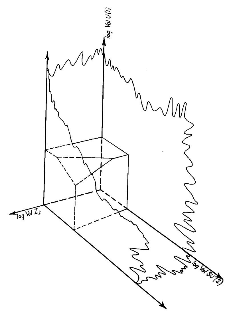
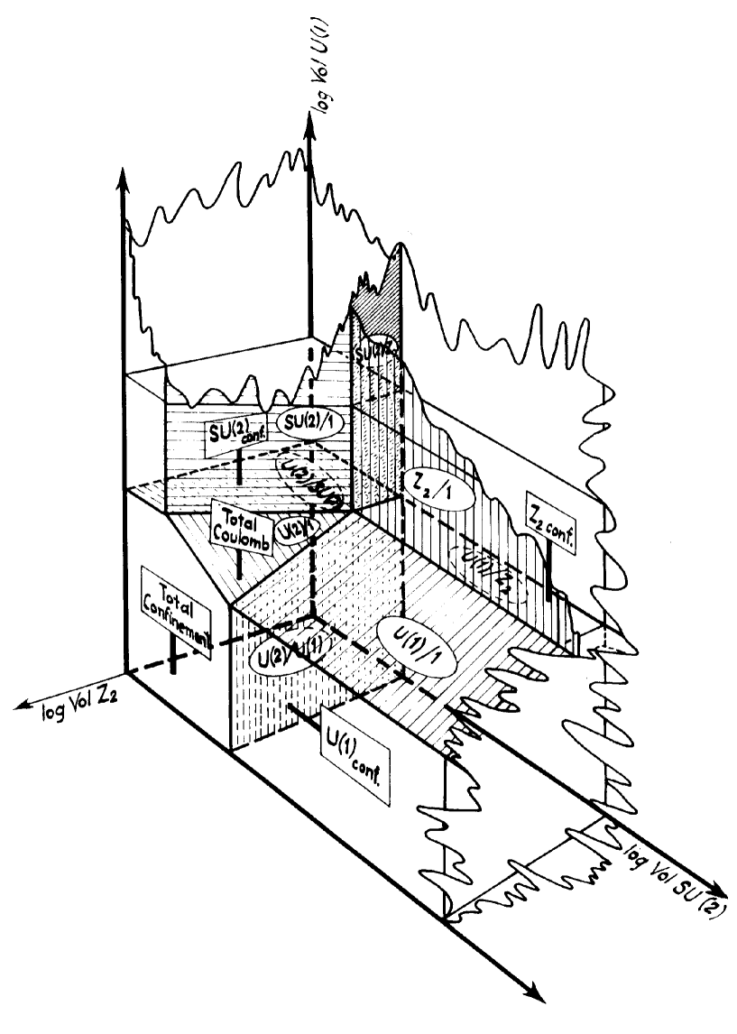
6.5.1 Need for discrete subgroup parameters

It is instructive to answer the question: Why do we need the discrete group action parameters? Recall that in our modified Manton action, there can be sharp “peaks” in the distribution $e^{S_{\Box}}$ of plaquette variables centred not only at the group identity but also at nontrivial elements of discrete subgroups. However, to motivate the answer to our question, we revert for a moment to an action $S_{\Box}$ leading to a distribution $e^{S_{\Box}}$ of plaquette variables with just one “peak” (at the identity) - this is just the normal Manton action. Then the quantities $Vol$ corresponding to the the same Lie algebra ideals in the Lie Algebra of the $SMG$ - i.e., volumes measured in units proportional to the fluctuation volume - obey the relations

$$\begin{array}[]{lcl}Vol(U(1)_{subgr.})&=&6Vol(SMG/(SU(2)\times SU(3)))\\ Vol(SU(2)_{subgr.})&=&2Vol(SMG/U(3))\\ Vol(SU(3)_{subgr.})&=&3Vol(SMG/U(2))\\ Vol(U(2)_{subgr.})&=&3Vol(SMG/SU(3))\\ Vol(U(3)_{subgr.})&=&2Vol(SMG/SU(2))\\ Vol(SU(2)\times SU(3))_{subgr.}&=&6Vol(SMG/U(1)).\end{array}$$ (204)

The important feature of this list is that each equality relates the quantity $Vol$ for a subgroup and factor group that both correspond to the same Lie algebra ideal (in the Lie algebra of the $SMG$). It is seen that $Vol$ for a subgroup with a given Lie algebra is larger than a factor group with the same Lie algebra by an integer factor equal to the number of centre elements of the subgroup that are identified in the factor group. It is important not to lose sight of the fact that quantity $Vol$ is, by definition, the volume of the group measured in the units proportional to the average group volume accessed by quantum fluctuations. This fluctuation volume is $\prod_{i\in\{U(1),SU(2),SU(3)\}}(2\beta_{i})^{-dim(i)/2}$ where it is understood that $i$ runs over the appropriate Lie sub-algebras. In the sequel, it is to be understood that when we refer to the volume of a group, we mean the quantity $Vol$.

Without the extra “peaks” of the modified Manton action, it is not possible to vary the volume on the left hand side of one of the equations (204) independently of the volume on the right hand side. For example, because of the (nontrivial) integer factor disparity in the volumes on the two sides of the equations (204), we cannot have $Vol(U(2)_{subgr.})=Vol(SMG/SU(3))$ at the same point in the $\beta$ parameter space. In particular, two such volumes can never have critical values for the same values of the $\beta$’s which means that the two corresponding partially confining phases (i,e., confinement w.r.t. $U(2)$ and $SU(3)$) cannot meet at a multiple point.

This feature is seen in Figure 19 which shows the phase diagram for the gauge group $U(2)$. In the plane defined by log$Vol(\mbox{\bf{Z}}_{2})=\log 2$ (the maximum value of log$Vol(\mbox{\bf{Z}}_{2})$), we have the phase diagram corresponding to the normal Manton action (one “peak” in the distribution of plaquette variables, centred at the identity; the fluctuation volume is accordingly also centred at the identity). Due to the fact that say $Vol(SU(2)_{subgr.})=2Vol(U(2)/U(1))$ (measured in the same unit of volume which is proportional to $\prod_{i\in\{U(1),SU(2),SU(3)\}}(2\beta_{i})^{-dim(i)/2}$), it is impossible to have $Vol(SU(2)_{subgr.})=Vol(U(2)/U(1))$ for the same values of the $\beta$ parameters; i.e., because the volumes of the subgroup and factor group corresponding to the same Lie algebra differ by a factor two, these two volumes cannot be critical for the same set of $\beta$ parameters. This in turn precludes phases partially confined w.r.t. $SU(2)$ and $U(1)$ from coming together. In the plane log$Vol(\mbox{\bf{Z}}_{2})=\log 2$ of Figure 19, it is indeed seen that these partially confining phases do not touch; the maximum number of phases that come together in this plane is three (i.e., not all four possible phases) where three is generic number of phases that can meet in two dimensions.

In order to succeed in having, for example, $Vol(SU(2)_{subgr.})=Vol(U(2)/U(1))$ in the case of the group $U(2)$, it is necessary to introduce a parameter that allows us to change the volume $Vol(SU(2)_{subgr.})$ without changing the volume of the Lie algebra-identical factor group $Vol(U(2)/U(1))$. In this $U(2)$ case, this is what is achieved by introducing the parameter log $Vol(\mbox{\bf{Z}}_{2})$ which allows the variation of the relative heights of the plaquette distribution “peaks” centred at the two elements of $\mbox{\bf{Z}}_{2}$.

By introducing an action giving rise to extra “peaks” in $e^{S_{\Box}}$ that are centred at elements that are (by definition) identified in a factor group but not in the subgroup having the same Lie algebra as the factor group, we admit the possibility of extra centres of fluctuation which increases the fluctuation volume (i.e., the unit in which $Vol$ is measured) for the subgroup but not for the factor group (because all centres of fluctuation are identified with the group identity in the factor group). Hence we gain a way of varying the volume of the subgroup (measured in fluctuation-volume units) without varying the volume of the factor group. In the example of $U(2)$ referred to above, the possibility of a peak in $e^{S_{\Box}}$ at the nontrivial element of $\mbox{\bf{Z}}_{2}$ in addition to the peak at the identity means that the total fluctuation volume for the subgroup $SU(2)$ can be made up of contributions from both peaks whereas the fluctuation volume of the Lie algebra-identical factor group $U(2)/U(1)$ can only come from the fluctuations centred at the identity since both elements of $\mbox{\bf{Z}}_{2}$ are identified in the factor group.

Relative to the approximate $U(2)$ phase diagram of Figure 19, the variation of the parameter log$Vol(\mbox{\bf{Z}}_{2})$ can be described roughly as follows. Recall from above that in the plane defined by log$Vol(\mbox{\bf{Z}}_{2})=\log 2$, there is only one “peak” in the distribution $e^{S_{\Box}}$ (centred at the identity). In this plane, the volume of the subgroup is, for given $\beta$ values, identically twice that of the factor group since there are by definition only half as many elements (i.e., cosets) in the factor group $U(2)/U(1)$ as there are elements in the subgroup $SU(2)$ with the same Lie algebra. Now as the value of the parameter log$Vol(\mbox{\bf{Z}}_{2})$ is reduced, the pattern of fluctuations changes in such a way that the nontrivial element of $\mbox{\bf{Z}}_{2}$ becomes a centre of quantum fluctuations with fluctuations that become progressively larger in the sense that more and more probability is relocated at the nontrivial element of $\mbox{\bf{Z}}_{2}$. However, fluctuations about the nontrivial element of $\mbox{\bf{Z}}_{2}$ are not “noticed” by the factor group because fluctuations about the identity and fluctuations about the nontrivial element correspond to fluctuations about the same coset of the factor group - namely the identity of the factor group. In our approximation, the parameter log$Vol(\mbox{\bf{Z}}_{2})$ decreases until the two peaks of $e^{S_{\Box}}$ (one at each element of $\mbox{\bf{Z}}_{2}$) have the same height and accordingly each contribute with half of the total fluctuation volume (i.e., the volume accessible to quantum fluctuations) of the subgroup $SU(2)$. This coincides with reaching the multiple point at which log$Vol(\mbox{\bf{Z}}_{2})=0$.

So at the multiple point, the unit of volume (i.e., the total fluctuation volume) used to measure the volume of the subgroup is just twice the fluctuation volume of the Lie algebra-identical factor group. This has the consequence that the volume of the subgroup $SU(2)$ is reduced by a factor two which is just the factor by which $VolSU(2)$ is larger than the Lie algebra-identical factor group $Vol(U(2)/U(1))$ in the absence of the extra parameter log$Vol(\mbox{\bf{Z}}_{2})$ that at the multiple point leads to a two-fold increase in fluctuation volume.

More generally, having discrete group action parameters allows the possibility of having a number of fluctuation centres in a subgroup that is just equal to the number of elements identified in going from a subgroup to the Lie algebra-identical factor group. At the multiple point, these additional centres increase the total fluctuation volume and thereby the unit of volume measurement for the subgroup relative to the fluctuation volume of the factor group by a factor equal to the number of elements identified in the factor group.

In summary, we have developed a generalised action that deals with the need for more than the usual number of parameters in the plaquette action if one wants to make the phases corresponding to confinement of the various invariant subgroups - including discrete (invariant) subgroups) share a common point (i.e., the multiple point) in the phase diagram. With our plaquette action parameterisation, we can show the existence of and also the coincidence in one multiple point of phases corresponding to all invariant subgroups of the non-Abelian components of the $SMG$. The invariant subgroups that we do not consider here correspond solely to additional discrete (invariant) subgroups of $U(1)$. The defining feature of a confinement-like phase for an invariant subgroup is equivalent to the assumption that Bianchi identity constraints can be neglected for such a phase in a crude weak coupling approximation using a mean field approximation.

At the multiple point, we are dealing with first order phase transitions; therefore, a priori at least, our multiple point principle suffers from lack of universality. However, the fact that a weak coupling approximation is at least approximately applicable - even for the determination of critical couplings - leads to the irrelevance of terms greater than second order in Taylor expansions of the action and consequently fosters the hope of an approximative universality.

6.6 Correction due to quantum fluctuations

In our model, the $SMG$ gauge coupling constants are to be identified with the couplings for the diagonal subgroup that results from the Planck scale breakdown of $SMG^{3}$. While in the naive continuum limit, the diagonal subgroup field configurations consist (by definition) of excitations that are identical for the $N_{gen.}=3$ copies (labelled by names $``Peter",\;``Paul",\cdots$) of any $SMG$ gauge degree of freedom $A^{b}_{\mu}$, a more realistic view must take into account that the $N_{gen.}$ copies of $A^{b}_{\mu}$ in $SMG^{3}$: $A^{b}_{\mu,\;Peter},A^{b}_{\mu,\;Paul},\cdots,A^{b}_{\mu,\;N_{gen.}}$ undergo quantum fluctuations relative to each other. In this section this correction is first estimated for a confinement-like phase (hereby justifying a disregard of Bianchi identities) and subsequently corrected so as to be approximately correct for a Coulomb-like phase.

Including the effect of fluctuations of a general quantum field $\theta$ in the continuum limit is done using the effective action $\Gamma[\theta_{cl.}]$:

$$\Gamma[\theta_{cl.}]=S[\theta_{cl.}]-\frac{1}{2}\mbox{Tr}(log(S^{{}^{\prime\prime}}[\theta_{cl.}])).$$ (205)

The correction to the continuum couplings that we calculate below consists in identifying the classical continuum action $\int d^{4}x\frac{-1}{4g^{2}}(gF_{\mu\nu}^{a})^{2}$ with the effective action $\Gamma$ - instead of with the lattice action $S$ - in the naive continuum limit approximation. In calculating this correction, we ignore non-Abelian effects and assume that the action $S_{{}_{Monte\;Carlo}}$ used in the literature[74, 73, 78] deviates only slightly from the Manton action for which the Tr$log$ correction is simply a constant. The $S_{Monte\;Carlo}$ could for example be the popular cosine action in the $U(1)$ case. First, however, we note that a change in the functional form of the action by $\delta S(\theta_{cl.})$ leads to a functional change in the effective action $\Gamma(\theta_{cl.})$ that differs from $\delta S(\theta_{cl.})$ by a term proportional to $\mbox{Tr}\frac{\delta S^{{}^{\prime\prime}}[\theta_{cl.}]}{S^{{}^{\prime\prime}}[\theta_{cl.}]}$:

$$\delta\Gamma[\theta_{cl.}]=\delta S[\theta_{cl.}]+\frac{1}{2}\mbox{Tr}(\delta(\log(S^{{}^{\prime\prime}}[\theta_{cl.}])))=\delta S[\theta_{cl.}]+\frac{1}{2}\mbox{Tr}(\frac{\delta(S^{{}^{\prime\prime}}[\theta_{cl.}])}{S^{{}^{\prime\prime}}[\theta_{cl.}]})$$ (206)

But as we are assuming that the variation $\delta S[\theta_{cl.}]$ is done relative to the Manton action, we have

$$\frac{1}{2}\mbox{Tr}(\frac{\delta(S^{{}^{\prime\prime}}[\theta_{cl.}])}{S^{{}^{\prime\prime}}_{Manton}[\theta_{cl.}]})=\frac{1}{2}\mbox{Tr}(S^{{}^{\prime\prime}}[\theta_{cl.}]\langle(\theta-\theta_{cl.})^{2}\rangle)$$ (207)

where we have used that $S^{{}^{\prime\prime}}_{Manton}[\theta_{cl.}]\propto\langle(\theta-\theta_{cl.})^{2}\rangle^{-1}=\;const.$ and that, up to a constant, $\delta(S^{{}^{\prime\prime}}[\theta_{cl.}])=S^{{}^{\prime\prime}}[\theta_{cl.}]$ (modulo a constant).

Neglecting non-Abelian effects, we generalise this result to non-Abelian gauge groups and write it more concretely using $U=e^{i\theta^{a}t^{a}}$ and $S[U]=\sum_{\Box}S_{\Box}(U(\Box))$:

$$\Gamma[U_{cl.}]=S[U_{cl.}]+\frac{1}{2}\Delta S_{\Box}(U_{cl.}(\Box))\langle(\theta_{\Box}^{a}(\Box)-\theta_{\Box\;cl.}^{a}(\Box))^{2}\rangle\;\;(\mbox{summation over}\;a)$$ (208)

We have for the Laplace-Beltrami operator

$$\frac{1}{2}\Delta S(U(\Box))\stackrel{{\scriptstyle def.}}{{=}}\lim_{\epsilon\rightarrow 0^{+}}\frac{\int d^{N^{2}-1}\!f\;\;\exp(-\frac{1}{2\epsilon}f_{a}^{2})(S(U\cdot e^{if_{b}t_{b}})-S(U))}{\int d^{N^{2}-1}\!f\;\;\exp(-\frac{1}{2\epsilon}f_{d}^{2})f_{e}^{2}}\;\;(\mbox{sum over }a,b,d,e).$$ (209)

where $f_{a}$ and $t_{a}$ denote respectively the $a$th Lie algebra component and Lie algebra generator. Upon expanding (in the representation $r$) the exponential $\exp(if_{b}T_{b,\,r})$ representing $\exp(if_{b}t_{b})$ the argument of which is assumed to be small inasmuch as the $f_{b}$ are assumed to be small, there obtains

$$=\lim_{\epsilon\rightarrow 0^{+}}\sum_{r}\frac{\beta_{r}}{d_{r}}\frac{\int d^{N^{2}-1}\!f\;\;\exp(-\frac{1}{2\epsilon}f_{a}^{2})\mbox{Tr}(U\cdot(-\frac{1}{2}f_{b}f_{c}T_{b,\,r}T_{c,\,r}))}{\int d^{N^{2}-1}\!f\;\;\exp(-\frac{1}{2\epsilon}f_{d}^{2})f_{e}^{2}}\;\;{\footnotesize(\mbox{sum over }a,b,c,d,e)}$$ (210)

$$=\sum_{r}\frac{\frac{\beta_{r}}{d_{r}}Tr_{r}(U\cdot(-\frac{1}{2}(T_{b,\,r})^{2}))}{N^{2}-1}\;\;(\mbox{sum over }b)$$ (211)

where we have expanded the plaquette action in characters: for the representation $r$ of dimension $d_{r}$ the character $\chi_{r}$ is given by $\chi_{r}=\mbox{Tr}_{r}(U(\Box))$ and

$$S(U(\Box))=\sum_{r}\frac{\beta_{r}}{d_{r}}\mbox{Tr}_{r}(U(\Box)).$$ (212)

We have

$$\frac{1}{2}\Delta S(U(\Box))=\sum_{r}-\frac{1}{2}\frac{\beta_{r}}{d_{r}}Tr_{r}(U(\Box))\frac{C^{(2)}_{r}}{N^{2}-1}$$ (213)

where $C^{(2)}_{r}$ is the quadratic Casimir for the representation $r$. The Casimir is defined as $C^{(2)}_{r}\mbox{\bf{1}}_{r}\stackrel{{\scriptstyle def.}}{{=}}\sum_{b}(T_{b,\;r})^{2}$. For the groups $SU(2)$ and $SU(3)$, the Lie algebra bases in the fundamental (defining) representations are taken respectively as $T_{b,\;r=f}=T_{b,\;r=\underline{\mbox{\scriptsize\bf{2}}}}=\frac{\sigma^{b}}{2}$ and $T_{b,\;r=f}=T_{b,\;r=\underline{\mbox{\scriptsize\bf{3}}}}=\frac{\lambda^{b}}{2}$. The subscript $f$ denotes the fundamental representation; $\sigma^{b}$ and $\lambda^{b}$ are the Pauli and Gell-Mann matrices with the normalisation $\mbox{Tr}(\frac{\sigma^{a}}{2}\frac{\sigma^{b}}{2})=\frac{\delta_{a}^{b}}{2}$ and $\mbox{Tr}(\frac{\lambda^{a}}{2}\frac{\lambda^{b}}{2})=\frac{\delta_{a}^{b}}{2}$. With this basis convention, and with the left-handed quark doublet field as an example, the covariant derivative is

$$D_{\mu i\;\;\;\alpha}^{\;\;\;\;j\;\;\,\beta}=\partial_{\mu}\delta_{i}^{\;\;j}\delta_{\alpha}^{\;\;\beta}-ig_{2}A_{\mu}^{b}\frac{(\sigma^{b})_{i}^{\;\;j}}{2}\delta_{i}^{\;\;j}-ig_{3}A_{\mu}^{b}\frac{(\lambda^{b})^{\;\;\beta}_{\alpha}}{2}\delta_{\alpha}^{\;\;\beta}-ig_{1}\frac{1}{6}A_{\mu}\delta_{i}^{\;\;j}\delta_{\alpha}^{\;\;\beta}.$$ (214)

where the index $b$ labels Lie algebra components, the indices $i,\;j$ label matrix elements of the ($2$-dimensional) fundamental representation of $SU(2)$, and the indices $\alpha,\;\beta$ label the matrix elements of the ($3$-dimensional) fundamental representation of $SU(3)$. The factor $\frac{1}{6}$ in the last term is the $U(1)$ quantum number $\frac{y}{2}$ where $y$ is weak hyper-charge; the convention used is $Q=\frac{y}{2}+I_{W_{3}}$.

The above convention for the generators of $SU(2)$ and $SU(3)$ in the fundamental representation $f$ leads to a Casimir $C^{(2)}_{f}=\frac{N^{2}-1}{2N}$ for an $SU(N)$ group. From this it follows that, for the adjoint representation (denoted by $adj.$), the Casimir $C^{(2)}_{adj.}$ for an $SU(N)$ group is given by $C^{(2)}_{adj.}=N$.

Ignoring Bianchi identities, we get for the deviations

$$\langle(\theta_{Peter}-\theta_{diag.})^{2}_{a}\rangle=\frac{N^{2}-1}{2}(\frac{1}{2}\sum_{r}\beta_{r}\frac{C^{(2)}_{r}}{N^{2}-1})^{-1}(\mbox{sum over }a)\mbox{ (confinement phase)}$$ (215)

$$=-\{\frac{\beta_{f}}{d_{f}}Tr_{f}(U_{diag.}(\Box))C^{(2)}_{f}+\frac{\beta_{adj.}}{d_{adj.}}Tr_{adj.}(U_{diag.}(\Box))C^{(2)}_{adj.}\}\frac{1}{2}\frac{N^{2}-1}{\beta_{f}C^{(2)}_{f}+\beta_{adj.}C^{(2)}_{adj.}}$$

Letting the sum over representations run only over the fundamental (=defining) and adjoint representations labelled respectively by the subscripts $f$ and $adj.$ (the only representations used in the Monte Carlo runs of references [74, 73, 78]), we get for the effective action (208)

$$\Gamma(U_{diag.}(\Box))=$$ (216)

$$=\frac{\beta_{f}}{d_{f}}Tr_{f}(U_{diag.}(\Box))(1-\frac{C^{(2)}_{f}(N^{2}-1)}{2(\beta_{f}C^{(2)}_{f}+\beta_{adj.}C^{(2)}_{adj.})})+\frac{\beta_{adj.}}{d_{adj.}}Tr_{adj.}(U_{diag.}(\Box))(1-\frac{C^{(2)}_{adj.}(N^{2}-1)}{2(\beta_{f}C^{(2)}_{f}+\beta_{adj.}C^{(2)}_{adj.})})$$

So with the continuum correction we have to make the replacement

$$\beta_{r}\rightarrow\beta_{r}(1-\frac{C^{(2)}_{r}(N^{2}-1)}{2\sum_{\hat{r}}\beta_{\hat{r}}C^{(2)}_{\hat{r}}})\;\;\mbox{(for ``confinement phase'')}$$ (217)

This expression for the effective action has been obtained using the approximation that all plaquette variables can be regarded as independent (i.e., Bianchi identities have been disregarded). This approximation is appropriate for the confinement phase. However, as we are interested in criticality as approached from the Coulomb phase (i.e., Coulomb phase in our scale dependent sense), we want the quantum fluctuation correction in this phase where Bianchi identities must be respected. These identities reduce the number of degrees of freedom per plaquette that can fluctuate independently by a factor 2. In going to the Coulomb phase, the continuum-corrected $\beta_{r}$ is modified as follows:

$$\beta_{r}(1-\frac{C^{(2)}_{r}(N^{2}-1)}{2\sum_{\hat{r}}\beta_{\hat{r}}C^{(2)}_{\hat{r}}})_{confinement}\rightarrow\beta_{r}(1-\frac{C^{(2)}_{r}(N^{2}-1)}{4\sum_{\hat{r}}\beta_{\hat{r}}C^{(2)}_{\hat{r}}})_{Coul.\;phase}$$ (218)

Without the continuum correction, we have for the fine structure constants at the multiple (i.e., triple ) point

$$\frac{1}{\alpha_{triple\;point,\,no\,cont.}}=4\pi\sum_{r}\frac{C^{(2)}_{r}\beta_{r,\,triple\;point}}{N^{2}-1}\;\;\mbox{(naive continuum limit)}.$$ (219)

With the continuum-corrected $\beta_{r}$ in the Coulomb phase we have for the fine structure constants at the triple point

$$\frac{1}{\alpha_{{}_{triple\;point,\,cont.}}}=4\pi\sum_{r}\frac{C^{(2)}_{r}}{N^{2}-1}\beta_{{}_{r\,triple\;point}}(1-\frac{C^{(2)}_{r}(N^{2}-1)}{4\sum_{\hat{r}}\beta_{{}_{\hat{r},\,triple\;point}}C^{(2)}_{\hat{r}}})=$$ (220)

$$4\pi\sum_{r}\frac{C^{(2)}}{N^{2}-1}\beta_{r\;triple\;point}(1-\pi C^{(2)}_{r}\alpha_{{}_{triple\;point,\;no\;cont.}})$$

6.7 Calculation of non-Abelian critical couplings at Planck scale

It can be argued that at the multiple point of the phase diagram for the whole $SMG^{3}=SMG\times SMG\times SMG$, the non-Abelian (plaquette) action parameters for each of the three Cartesian product factors take the same values as at the multiple point for a single gauge group $SMG$. This allows us to determine the multiple point action parameters for the gauge group $SMG^{3}$ from a knowledge of the multiple point action parameters for just one of the $SMG$ factors of $SMG^{3}$. Accordingly, we can calculate the multiple point critical couplings from the couplings for the isolated $SU(2)$ and $SU(3)$ groups. To this end, we have used figures from the literature [74, 73, 79] to graphically extract the coordinates $(\beta_{f},\beta_{adj.})_{triple\;point}$ of the triple point:

For $SU(2)$: $(\beta_{f},\beta_{adj.})_{triple\;point}=(0.54,2.4)$

For $SU(3)$: $(\beta_{f},\beta_{adj.})_{triple\;point}=(0.8,5.4)$

Table 4:

Table 4: SU(2) Gauge Coupling
Prediction for continuum limit coupling estimate, $1/\alpha_{2,\;triple\;point,\;cont.}$, using
1. not exponentiated:	$\overbrace{0.71\cdot 20}^{14.2}+\overbrace{0.89\cdot 1.7}^{1.5}=15._{7}\pm 1$
2. exponentiated:	$\overbrace{0.75\cdot 20}^{15._{0}}+\overbrace{0.89\cdot 1.7}^{1.5}=16._{5}\pm 1$
Experimental value[24, 25] for
$1/\alpha_{2}$ reduced by a factor 3:	$\frac{1}{3}\cdot\alpha^{-1}_{2}(M_{Z})=\frac{1}{3}\cdot(29.7\pm 0.2)=9.9\pm 0.07$
“desert extrapolation[24, 25]” to
Planck scale with one Higgs:	$\stackrel{{\scriptstyle desert}}{{\longrightarrow}}\frac{1}{3}\cdot\alpha^{-1}_{2}(\mu_{Pl.})=\frac{1}{3}\cdot 49._{5}=16.5$
$\beta_{adj.,\;triple\;point}$ (i.e., at triple point)	2.4 (ca. 5% uncertainty from MC)
$\beta_{f\;triple\;point}$ (i.e., at triple point)	0.54 (ca. 10% uncertainty from MC)
$\beta_{adj.}$-contribution to $1/\alpha_{2,\;triple\;point}$
(without continuum correction)	$4\pi\frac{C^{(2)}_{adj.}}{(2^{2}-1)}\beta_{adj,\;triple\;point}=4\pi\cdot(2/3)\cdot 2.4=20$
$\beta_{f}$-contribution to  $1/\alpha_{2,\;triple\;point}$
(without continuum correction):	$4\pi\frac{C^{(2)}_{f}}{(2^{2}-1)}\beta_{f\;triple\;point}=4\pi\cdot(\frac{3}{4}/3)\cdot 0.54=1.7$
Full $1/\alpha_{2,\;triple\;point}$ (without continuum
correction):	$1/\alpha_{2,\;triple\;point,\;full,\;no\;cont.}=20+1.7=21.7$
Continuum correction factor for $\beta_{adj.}$-contribution:
1. not exponentiated (using (220)):	$1-C^{(2)}_{adj.}\pi\alpha_{2,\;triple\;point,\;full,\;no.\;cont.}=$
	$1-2\pi/21.7=1-0.290=0.71$
2. exponentiated:	$\exp(-C^{(2)}_{adj.}\pi\alpha_{2,\;triple\;point,\;full,\;no.\;cont.})$=
	$\exp(-2\pi/21.7)=\exp(-0.290)=0.75$
Continuum correction factor for $\beta_{f}$-contribution:
1. not exponentiated (using (220)):	$1-C^{(2)}_{f}\pi\alpha_{2,\;triple\;point,\;full,\;no.\;cont.}=$
	$1-(\frac{3}{4})\pi/21.7=1-0.109=0.89$
2. exponentiated:	$\exp(-C^{(2)}_{f}\pi\alpha_{2,\;triple\;point,\;full,\;no.\;cont.})=$
	$\exp(-(\frac{3}{4})\pi/21.7)=\exp(-0.109)=0.90$

Table 5:

Table 5: SU(3) Gauge Coupling
Prediction for continuum limit coupling estimate, $1/\alpha_{3,\;triple\;point,\;cont.}$, using
1. not exponentiated:	$\overbrace{0.65\cdot 25}^{16._{3}}+\overbrace{0.84\cdot 1.7}^{1.4}=17._{7}\pm 1$
2. exponentiated:	$\overbrace{0.70\cdot 25}^{17._{5}}+\overbrace{0.85\cdot 1.7}^{1.4}=18._{9}\pm 1$
Experimental value[24, 25] for
$1/\alpha_{3}$ reduced by a factor 3:	$\frac{1}{3}\cdot\alpha^{-1}_{3}(M_{Z})=\frac{1}{3}\cdot(8.47\pm 0.5)=2.8\pm 0.2$
“desert extrapolation[24, 25]” to
Planck scale with one Higgs:	$\stackrel{{\scriptstyle desert}}{{\longrightarrow}}\frac{1}{3}\cdot\alpha^{-1}_{3}(\mu_{{}_{Pl.}})=\frac{1}{3}\cdot 53\pm 0.7=17.7\pm 0.3$
$\beta_{adj.,\;triple\;point}$ (i.e., at triple point)	5.4 (ca. 5% uncertainty)
$\beta_{f\;triple\;point}$ (i.e., at triple point)	0.8 (ca. 20% uncertainty)
$\beta_{adj.}$-contribution to $1/\alpha_{3,\;triple\;point}$
(without continuum correction)	$4\pi\frac{C^{(2)}_{adj.}}{(3^{2}-1)}\beta_{adj,\;triple\;point}=4\pi\cdot(3/8)\cdot 5.4=25$
$\beta_{f}$-contribution to  $1/\alpha_{3,\;triple\;point}$
(without continuum correction):	$4\pi\frac{C^{(2)}_{f}}{(3^{2}-1)}\beta_{f\;triple\;point}=4\pi\cdot(\frac{4}{3}/8)\cdot 0.8=1.7$
Full $1/\alpha_{3,\;triple\;point}$ (without continuum
correction):	$1/\alpha_{3,\;triple\;point,\;full,\;no\;cont.}=25+1.7=26._{7}$
Continuum correction factor for $\beta_{adj.}$-contribution:
1. not exponentiated (using (220)):	$1-C^{(2)}_{adj.}\pi\alpha_{3,\;triple\;point,\;full,\;no.\;cont.}=$
	$1-3\pi/26.7=1-0.35=0.65$
2. exponentiated:	$\exp(-C^{(2)}_{adj.}\pi\alpha_{3,\;triple\;point,\;full,\;no.\;cont.})$=
	$\exp(-3\pi/26.7)=\exp(-0.35)=0.70$
Continuum correction factor for $\beta_{f}$-contribution:
1. not exponentiated (using (220)):	$1-C^{(2)}_{f}\pi\alpha_{3,\;triple\;point,\;full,\;no.\;cont.}=$
	$1-(\frac{4}{3})\pi/26.7=1-0.16=0.84$
2. exponentiated:	$\exp(-C^{(2)}_{f}\pi\alpha_{3,\;triple\;point,\;full,\;no.\;cont.})=$
	$\exp(-(\frac{4}{3})\pi/26.7)=\exp(-0.16)=0.85$

The calculation of $\alpha_{2}^{-1}$ and $\alpha_{3}^{-1}$ are presented in Tables 4 and 5 respectively. In these tables, the subscripts ${adj.}$ and $f$ denote respectively the adjoint and fundamental representations of the groups considered.

In order to get an idea of the order of magnitude of the error involved in estimating the average over the Laplace-Beltrami of the plaquette action only to next to lowest order, we note that we can calculate such an average to all orders in the case of a $\cos\theta$ action for a $U(1)$ gauge theory. In this case the averaging is readily performed and leads to an exponential for which the first terms of a Taylor expansion coincide with the terms we calculated using (220). This suggests that also in the non-Abelian cases it might be quite reasonable to “exponentiate” our “continuum” corrections and subsequently use the change made by such a procedure as a crude estimate of the error due to our omission of the second order perturbative terms. By exponentiated continuum corrections we mean by definition that, instead of the replacements (217) and (218), we use respectively

$$\beta_{r}\rightarrow\beta_{r}\exp(-\frac{C^{(2)}_{r}(N^{2}-1)}{2\sum_{\hat{r}}\beta_{\hat{r}}C^{(2)}_{\hat{r}}}\;\;\;\mbox{(for ``confinement'')}$$ (221)

and

$$\beta_{r}\rightarrow\beta_{r}\exp(-\frac{C^{(2)}_{r}(N^{2}-1)}{4\sum_{\hat{r}}\beta_{\hat{r}}C^{(2)}_{\hat{r}}}\;\;\;\mbox{(for ``Coulomb'' phase)}$$ (222)

As evidenced by Tables 4 and 5, this exponentiation yields a change of the order of one unit in $1/\alpha_{crit.,\;cont.}$ $\approx$ 20 from which we can estimate the uncertainty due the neglect of higher order terms as being of the order of say 5 %.

Since our deviations from the experimental couplings extrapolated to the Planck scale[24, 25] are of the same order of magnitude as the uncertainty in the Monte Carlo data and the uncertainty due to chopping off the higher order continuum corrections, a calculation of the next order corrections and increased accuracy in the calculations are called for in order to determine if our deviations are significant.

theu1b.tex 31 May 96 alf

7 Implementing the MPCP in determining the SMG U(1) coupling: Methods for constructing phase diagrams

The gauge group to which we ultimately want to apply the Multiple Point Criticality Principle (MPCP) is the Anti Grand Unified Theory (AGUT) gauge group $SMG^{3}$ or some group in which the latter is embedded in such a way that $SMG^{3}$ dominates as the group to be considered. However for the purpose of finding the multiple point $U(1)$ coupling, it can be argued that we can approximately ignore the interaction between the Abelian and non-Abelian subgroups provided we identify the $U(1)_{i}$ factors in $U(1)^{3}$ with the factor groups $SMG_{i}/(SU(2)\times SU(3))_{i}$ $(i\in\{Peter,Paul,Maria\})$. In this approximation, we essentially treat $SU(3)^{3}$, $SU(2)^{3}$ and $U(1)^{3}$ separately. We shall now address the $U(1)$ degrees of freedom by endeavouring the construction of some rather rough approximations to the phase diagram for a lattice gauge theory with the gauge group $U(1)^{3}$. In order to provoke the many possible phases $(K,H)$, including in principle the denumerable infinity of “phases” involving the discrete subgroups of $U(1)^{3}$, it is necessary to use a functional form for the plaquette action that is quite general.

7.1 Special problems with $U(1)^{3}$

In the case of the non-Abelian subgroups of the $SMG$ that we have dealt with in earlier work[3, 4], the correction factor in going from the multiple point couplings of $SMG^{3}$ to the diagonal subgroup couplings is 3 corresponding to the value of the number of generations $N_{gen}$. Recall that the diagonal subgroup couplings are in our model predicted to coincide with the experimental $U(1)$ coupling after extrapolation to the Planck scale.

However, the relation of the diagonal subgroup couplings to the multiple point critical couplings in the case of $U(1)^{3}$ turns out to be more complicated than for the non-Abelian $SMG$ couplings. The resolution of these complications helps us to understand the phenomenological disagreement found when a naively expected correction factor of $N_{gen}=3$ is used in going from the $U(1)$ couplings at the multiple point of $U(1)^{3}$ to the couplings for the diagonal subgroup of $U(1)^{3}$.

For the fine-structure constants of the non-Abelian groups $SU(2)$ and $SU(3)$, it was found that experimental values extrapolated to the Planck scale agree to within the uncertainties of our calculation with the predicted values $1/\alpha_{diag\;multicr}=3/\alpha_{multicr.}$ (i.e. the inverse fine-structure constants for the diagonal subgroups of the non-Abelian subgroups of $SMG^{3}$). While the factor 3 correction to the multiple point inverse squared coupling values obtained for a lattice gauge theory yields rather noteworthy agreement with the experimental values of non-Abelian fine-structure constants, the analogous relation does not hold for the $U(1)$ gauge algebra (weak hyper-charge). For $U(1)$ a correction factor of roughly 6 (or 7) is indicated phenomenologically. This would naively suggest that at the Planck scale we should postulate something like

$$U(1)^{6\;or\;7}=\overbrace{U(1)\times\cdots\times U(1)}^{6\;or\;7\;factors}$$ (223)

rather than $U(1)^{3}$ as suggested by our preferred “fundamental” gauge group $SMG^{N_{gen}}$ with $N_{gen}=3$.

An explanation for this disparity when we use $U(1)^{3}$ as the gauge group (rather than the naively indicated $U(1)^{6}$ or $U(1)^{7}$) can be sought by considering how the “Abelian-Ness” of $U(1)$ distinguishes it from the non-Abelian subgroups.

7.1.1 The normalisation problem for $U(1)$

For $U(1)$, there is no natural unit of charge in contrast to the non-Abelian groups $SU(2)$ and $SU(3)$. For these latter, there is a way to normalise the fine-structure constants by means of the commutators. The commutation algebra provides a means of unambiguously fixing a convention for the gauge couplings that alone pertains to the Yang-Mills fields without reference to the charge of, for example, a matter field; the Yang-Mills fields are themselves charged in the non-Abelian case and can therefore be used to define a charge convention. Essentially this is because the Lie algebra commutator relations are non-linear and are therefore not invariant under re-scalings of the gauge potential $g{\bf A}_{\mu}$. Such scalings, if not forbidden, would of course deprive gauge couplings of physical significance.

Because such a rescaling is possible in the case of $U(1)$, the weak hyper-charge fine-structure constant is only normalizable by reference to some quantum of charge. This immediately raises the question of which particle should be declared as having the unit quantum of charge as its hyper-charge. An equivalent way to address this question is to ask which $U(1)$-isomorphic factor group of $SMG$ should be identified with the $U(1)$ on the lattice to give us the critical coupling.

It is only when - on the lattice - the group of real numbers R (in the covering group $\mbox{\bf{R}}\times SU(2)\times SU(3)$ of the $SMG$) is compactified to a $U(1)$ that a normalisation becomes possible and thereby that the idea of a critical coupling acquires a meaning. The only remnant in the continuum of having chosen a specific group on the lattice is the quantisation rule of the charges (more generally, a constraint on the allowed representations) and the lattice artifact monopoles. This suggests that we should take the length of the $U(1)$ in such a way as to enforce empirical charge quantisation rules. When we state that the critical coupling for a $U(1)$ lattice gauge theory is given by

$$\alpha_{crit}\propto\frac{1}{4\pi\beta_{crit}}=\frac{1}{4\pi\cdot 1.01},$$ (224)

the meaning is that this $\alpha_{crit}$ is the fine-structure constant at the phase transition corresponding to the coupling to the smallest charge quantum allowed on the lattice. For the $SMG$ as we define it:

$$SMG\stackrel{{\scriptstyle def}}{{=}}S(U(2)\times U(3))\stackrel{{\scriptstyle def}}{{=}}(\mbox{\bf{R}}\times SU(2)\times SU(3))/\{(2\pi,\mbox{\bf{1}}^{2\times 2},e^{i\frac{2\pi}{3}}\mbox{\bf{1}}^{3\times 3})^{n}|n\in\mbox{\bf{Z}}\},$$ (225)

the charge quantisation rule for weak hyper-charge is very sophisticated[30, 31, 80]:

$$y/2+d/2+t/3=0\;\;(\mbox{mod }1).$$ (226)

This means that depending on whether the non-Abelian subgroups are represented trivially or non-trivially, the smallest allowed quantum for the weak hyper-charge is respectively $y/2=1$ and $y/2=1/6$. This complicated quantisation rule can be regarded as a consequence of Nature having chosen the gauge group[19, 81] $S(U(2)\times U(3))$. In spite of the fact that the global structure of this group imposes the severe restriction (226) on the possible representations, it still allows all representations that are seen phenomenologically.

The $U(1)$ centre of $SMG$ is embedded in the latter in a complicated way. In order to determine the non-Abelian coupling of the $SMG$, one must relate the $U(1)$ centre of the $SMG$ and the simple $U(1)$ studied using Monte Carlo methods on a lattice. Our earlier work suggests that the disconnected $\mbox{\bf{Z}}_{2}$ and $\mbox{\bf{Z}}_{3}$ centres of respectively the non-Abelian $SMG$ subgroups $SU(2)$ and $SU(3)$ should both alone be confined in phases that convene at the multiple point. In order to respect this requirement in the present work, it is necessary to require that the class of $\mbox{\bf{Z}}_{N}$ discrete subgroups $\mbox{\bf{Z}}_{N}$ for which there can be phases convening at the multiple point that are solely confined along $\mbox{\bf{Z}}_{N}$ must be as follows: when $\mbox{\bf{Z}}_{K}$ is in this class, then so are the groups $\mbox{\bf{Z}}_{K}+\mbox{\bf{Z}}_{2}=\mbox{\bf{Z}}_{K^{\prime}}$ (where $K^{\prime}$ is the smallest integer multi-plum of $K$ that is divisible by 2) and the groups $\mbox{\bf{Z}}_{K}+\mbox{\bf{Z}}_{3}=\mbox{\bf{Z}}_{K^{\prime\prime}}$ (where $K^{\prime\prime}$ is the smallest integer multi-plum of $K$ divisible by 3). Hence, for the phases that convene at the multiple point, the greatest $N$ of a phase that is solely confined w.r.t a subgroup $\mbox{\bf{Z}}_{N}$ must be such that $N$ is divisible by 2 and 3 and thus also by 6.

A rule from our earlier work[71] states that the coupling for a continuous Lie (sub)group $L$ at the multiple point is given - to a good approximation - by the critical coupling for a the factor group $L/\mbox{\bf{Z}}_{N_{max}}$ anywhere along the phase border where the Coulomb-like degrees of freedom corresponding to this factor group are critical. Here $\mbox{\bf{Z}}_{n_{max}}$ denotes the largest discrete subgroup that alone confines in a phase that convenes at the multiple point. We shall refer to this rule as the $\mbox{\bf{Z}}_{N_{max}}$ factor group rule.

We shall argue below that the largest discrete subgroup of the $U(1)$ centre of $SMG$ that is solely confined in a phase that convenes at the multiple point does not result in a $U(1)$-isomorphic factor group of length shorter than that corresponding to the identification of $SU(2)\times SU(3)$ with the identity. This corresponds to dividing the largest possible non-Abelian subgroup out of the $SMG$; the result is a factor group isomorphic with $U(1)/\mbox{\bf{Z}}_{6}$:

$$U(1)/\mbox{\bf{Z}}_{6}\stackrel{{\scriptstyle-}}{{\simeq}}SMG/(SU(2)\times SU(3)).$$ (227)

Consequently, we shall also argue that the $U(1)$ critical coupling $\sqrt{4\pi\alpha_{crit}}$ obtained using Monte Carlo simulations of a $U(1)$ lattice gauge theory is to be identified with the charge quantum of the factor group $SMG/(SU(2)\times SU(3))$. Subsequently we shall substantiate that it is reasonable to take this charge quantum as the weak hyper-charge of the left-handed positron (i.e., $y/2=1$). The arguments for this choice are indeed pivotal for the credibility of the proposed model. Had we for example taken the lattice critical coupling $\sqrt{4\pi\alpha_{crit}}$ as the hyper-charge of the left-handed quarks - which are assigned to the $\underline{2}\otimes\underline{3}$ representation of $SU(2)\times SU(3)$:

$$\left(\begin{array}[]{ccc}u_{r}&u_{b}&u_{y}\\ d_{r}^{c}&d_{b}^{c}&d_{y}^{c}\end{array}\right),$$ (228)

this would lead to an $\alpha_{crit}(\mu_{Pl})$ that was a factor $6^{2}=36$ times larger than that obtained the left-handed positron.

We return to these matters in Section 7.1.3.

7.1.2 The infinity of discrete subgroups of $U(1)^{3}$

Recall that at the multiple point, there are, in addition to phases confined w.r.t. continuous subgroups, also phases that are confined solely w.r.t. discrete subgroups. We use as the definition of confinement that Bianchi identities can be disregarded in the sense that plaquette variables can be treated as independent variables. We define Bianchi variables to be the group product of the plaquette variables enclosing a 3-volume. The simplest Bianchi variable on a hyper-cubic lattice are the 3-cubes enclosed by six plaquettes. Bianchi variables are identically equal to the group identity. This constraint introduces in general correlations between the values taken by plaquettes forming the boundary of a 3-volume. In the case of a first order phase transition, there is a “jump” in the width of the distribution of plaquette variables in going from a Coulomb to a confining phase. Our claim is that this “jump” is explained by a change in how effective Bianchi identities are in enforcing correlations between plaquette variable distributions for different plaquettes forming the closed surface of a 3-volume. In the Coulomb phase, Bianchi identities can presume-ably only be satisfied by having the sum of phases (thinking now of $U(1)$) of the plaquettes bounding a 3-volume add up to zero. At the transition to a confining phase, the width of plaquette variable distributions is large enough so that Bianchi identities are readily fulfilled in any of a large number of ways in which the values of plaquette variables can sum to a non-zero multiple of $2\pi$. This greater ease (energetically) with which Bianchi identities can be satisfied for a variety of configurations of values of boundary plaquette variables means that Bianchi identities are less effective in causing correlations between plaquette variables which in turn allows even greater fluctuations in plaquette variables in a sort of chain reaction that we claim is the explanation for the sudden decrease in the Wilson loop operator at the Coulomb to confining phase transition.

Were it not for Bianchi identities, the distributions of values taken by Bianchi variables would correspond (for a simple 6-sided cube) to the 6-fold convolution of an independent plaquette variable distribution (i.e., uncorrelated with the distribution on other plaquettes). For such a distribution, it turns out that the critical value of the inverse squared coupling coincides with a change from a distribution centred at the group identity to an essentially “flat” (i.e., Haar measure) distribution. That the 6-fold convolution of independent plaquette variable distributions becomes rather“flat” at the critical value of the coupling concurs nicely with our characterisation of confinement as the condition that prevails when the fulfilment of Bianchi identities has become almost “infinitely easy” energetically and can therefore be neglected in the sense that plaquette variable distributions for different plaquttes can be taken as approximately independent.

If it is a discrete subgroup that is confined, there will be subsidiary peaks in the exponentiated plaquette action $e^{S_{\Box}}$ at nontrivial elements of this discrete subgroup. Confinement occurs just when the subsidiary peaks are accessed with sufficient probability so that the 6-fold convolution of the plaquette distribution over elements of the discrete subgroup leads to comparable probabilities for accessing all of these discrete subgroup elements (i.e., when the 6-fold convolution of a plaquette variable distribution takes values at all elements of the discrete subgroup with roughly the same probability).

Having in the plaquette distribution the presence of subsidiary peaks (i.e., maxima of the distribution of group elements) at nontrivial elements of discrete subgroups affects the value of the critical coupling of the continuous (i.e., Lie) group degrees of freedom at the Coulomb to confinement phase transition. However, once the discrete subgroup is in the confining phase, the dependence of the Lie group critical coupling on the relative heights of the peaks has essentially reached a plateau. This is so because fluctuations along the discrete subgroup are by definition large enough so that the transition-relevant distribution obtained as the 6-plaquette convolution of the plaquette distribution over the discrete group is essentially already flat so that going deeper into confinement will hardly access more elements of the Lie group. So the Lie group coupling is essentially unchanged in going from the multiple point to where the discrete subgroup is deeply confined (meaning parameter values for which the discrete peaks are equally high). Here the fluctuations along the discrete subgroup and the cosets that are translations of it are maximal (i.e., equal probabilities for all the elements in a coset) and one therefore needs effectively only to consider the factor group obtained by dividing out the discrete subgroup. This is the reasoning underlying the $\mbox{\bf{Z}}_{N_{max}}$ factor group rule discussed above. The rule states that to a good approximation, the multiple point continuous group coupling equals the critical coupling for this factor group.

7.1.3 Resolving the $U(1)$ normalisation problem

There is the problem with $U(1)$ that the principle of multiple point criticality suggests that there should even be phases convening at the multiple in which there is solely confinement of $\mbox{\bf{Z}}_{N}$ subgroups of arbitrarily large $N$. This would result in couplings that vanish. However, if we also give the matter fields some arbitrarily large number of the charge quanta of the $U(1)$ that corresponds to the lattice compactification of R, the coupling of these matter particles need not be zero. But then our prediction would (only) be that the matter coupling is a rational number times the multiple point critical coupling.

In order to suggest the manner in which this rational factor might arise, let us speculate in terms of a model for how our universe came about. First we describe the model; then we formulate two concise statements from which the model follows. We end this Section by arguing for the validity of the two statements.

Assume that at high temperatures (e.g. immediately following the“Big Bang”), the phase that dominates is that having the largest number of light particles. Recalling that the various phases convening at the multiple point have the same vacuum energy density (in Minkowski language), such a phase would constitute the ”highest pressure” phase that could be expected to expand at the expense of other phases. We speculate that such a phase has an optimal balance of unconfined fermions and unconfined monopoles. However, unconfined monopoles are present in phases that are confined w.r.t. discrete subgroups (i.e., $\mbox{\bf{Z}}_{N}$ subgroups). So in terms of our speculative picture, we do not expect the high temperature dominant phase to be a totally Coulomb-like phase but rather a phase confined w.r.t. some discrete subgroups. In this scenario, we would claim that the phase in which we live - “our” cold-universe phase - has the maximal number of monopole charges consistent with having the phenomenologically known electrically charged particles (quarks and leptons). This leads us to a system of monopoles (in “our” cold-universe phase) causing confinement for any fraction of the electric charges known to exist phenomenologically. The picture to have in mind is that “our” cold-universe phase is but one of many degenerate phases that can convene at the multiple point of a cold universe. We speculate that the reason that only our phase is realized is because “our” phase dominated so effectively at the high temperatures following the “Big Bang” that all other phases disappeared with the result that these phases are non-existent in the present low-temperature universe. Had there existed “seeds” of these phases in the present universe, they could have competed more or less successfully with “our” phase.

Let us examine this proposal for “our” universe in the context of a $U(1)$ lattice gauge theory. We denote by the symbol $U(1)_{fund}$ the $U(1)$ gauge group that is associated with the compactification that establishes the Abelian degrees of freedom on the fundamental lattice. Let us furthermore assume that there is some integer $N_{max}$ such that $\mbox{\bf{Z}}_{N_{max}}$ is the largest discrete subgroup of $U(1)_{fund}$ that can confine alone in one of the phases convening at the cold-universe multiple point. This corresponds to having Coulomb-like behaviour for the coset-degrees of freedom of the factor group $U(1)_{fund}/\mbox{\bf{Z}}_{N_{max}}$. This means that if a $\mbox{\bf{Z}}_{N}$ with $N>N_{max}$ confines in a phase that convenes at the multiple point, it does so not alone but because the continuous $U(1)$ degrees of freedom also confine. Finally, let $N_{our}$ be defined such that $\mbox{\bf{Z}}_{N_{our}}$ is the largest discrete subgroup that alone is confined in “our” phase (which is assumed to be among the phases that meet at the multiple point).

With the assumption of an $N_{max}$, we can immediately conclude that the $U(1)_{fund}/\mbox{\bf{Z}}_{N_{max}}$ representation of $U(1)_{fund}$ has the largest minimum allowed charge quantum. Let us denote this as $Q_{max}$. Furthermore, we can conclude that the smallest allowed charge quantum - namely that of $U(1)_{fund}$ - is $Q_{max}/N_{max}$.

In terms of monopoles, we have of course the dual situation: denoting the smallest allowed monopole charge for $U(1)_{fund}$ as $m_{fund}$, the factor group $U(1)_{fund}/\mbox{\bf{Z}}_{N_{max}}$ allows monopoles of fractional charge the only restriction being that these must be multiples of $m_{fund}/N_{max}$.

The above proposal for “our” cold-universe phase as a vacuum that allows monopoles causing confinement for any fraction of the electric charges (measured in charge quanta of $U(1)_{fund}$) known to exist phenomenologically follows as a consequence of the validity of two statements:

1. $N_{our}$ and $N_{max}$ are such that:

   $$N_{max}=6\cdot N_{our}$$

   $$N_{our}\mbox{ not divisible by 2 or 3.}$$

2. The critical coupling $e_{crit}=\sqrt{4\pi\alpha_{crit}}$ for a $U(1)$ lattice gauge theory determined using Monte Carlo methods should be identified with the charge quantum $Q_{max}$ of the factor group $U(1)_{fund}/\mbox{\bf{Z}}_{N_{max}}$.

Before substantiating these statements, we first discuss some conclusions that that follow from assuming the validity of them.

As long as the conditions of statement 1 are fulfilled, $N_{max}$ can be arbitrarily large without making the coupling at the multiple point vanish (see first paragraph of (this) Section 7.1.3). The smallest allowed charge quantum in “our” phase is $N_{our}(Q_{max}/N_{max})\stackrel{{\scriptstyle def}}{{=}}Q_{our}$; the discrete subgroups $\mbox{\bf{Z}}_{2}$ and $\mbox{\bf{Z}}_{3}$ are not confined in “our” phase. These discrete subgroups $\mbox{\bf{Z}}_{2}$ and $\mbox{\bf{Z}}_{3}$ - which are only found once as subgroups of $\mbox{\bf{Z}}_{N_{max}}$ - are confined (alone) only in phases to which are associated minimum allowed charge quanta larger than $Q_{our}$. Using the statement 2, we can fix the value of the smallest allowed charge quantum in the phase with $/bz_{N_{max}}$ alone confined as $\sqrt{4\pi\alpha_{crit}}$ and thus in “our” phase as $Q_{our}=N_{our}\cdot(\sqrt{4\pi\alpha_{crit}}/N_{max})$.

It is now necessary to give an argument for which physical particles should have $Q_{max}=\sqrt{4\pi\alpha_{crit}}$ as its charge quantum. As stated above, earlier work leads us to expect the $\mbox{\bf{Z}}_{2}$ and $\mbox{\bf{Z}}_{3}$ centres of respectively $SU(2)$ and $SU(3)$ to confine alone in phases convening at the multiple point. The phase with $\mbox{\bf{Z}}_{2}\times\mbox{\bf{Z}}_{3}$ confined alone coincides with the phase with Coulomb-like behaviour for the coset degrees of freedom of the factor group $SMG/(SU(2)\times SU(3))\stackrel{{\scriptstyle-}}{{\simeq}}U(1)/\mbox{\bf{Z}}_{6}$ corresponding to the trivial representation of the $SU(2)\times SU(3)$ degrees of freedom. The left-handed positron $e^{+}_{L}$ is the singlet under $SU(2)\times SU(3)$ that has the smallest charge.

At the end of this Section, we shall give a speculative argument for why it is natural that the phase in which there alone is confinement of $SMG/(SU(2)\times SU(3))\stackrel{{\scriptstyle-}}{{\sim}}U(1)/\mbox{\bf{Z}}_{6}$ should be identified with the phase in which there is confinement solely of the discrete subgroup $\mbox{\bf{Z}}_{N_{max}}$ corresponding to Coulomb-like degrees of freedom for the cosets of $\frac{U(1)_{fund}/{\mbox{\scriptsize\bf{Z}}}_{N_{our}}}{\mbox{\bf{Z}}_{6}}\ =U(1)_{fund}/\mbox{\bf{Z}}_{N_{max}}$. This identification puts the hyper-charge of the left-handed positron into correspondence with the factor group $U(1)_{fund}/\mbox{\bf{Z}}_{N_{max}}$ charge quantum $\sqrt{4\pi\alpha_{crit}}$.

Use now the usual convention for hyper-charge: $y/2=Q/6Q_{L}$ (for particles of hyper-charge $Q$) and associate $(y/2)_{e^{+}_{L}}=1$ with $Q=Q_{max}=\sqrt{4\pi\alpha_{crit}}$ (the $U(1)$ lattice gauge critical coupling). This determines the hyper-charge quantum $Q_{L}$ of “our” phase (which has unconfined quarks and leptons at the Planck scale) as $Q_{L}=\frac{\sqrt{4\pi\alpha_{crit}}}{6}$. This is the charge quantum of the $\underline{2}\otimes\underline{3}$ representation of $SU(2)\times SU(3)$.

The properties ascribed to “our” cold-universe phase are contingent upon the validity of statements 1 and 2 above. Let us now argue for the validity of these statements (in reverse order).

Statement 2 follows basically from the $Z_{N_{max}}$ factor group rule for the multiple point coupling of continuous degrees of freedom as discussed on page 7.1.3. This rule states that if the multiple point for $U(1)_{fund}$ has contact with a phase in which a discrete subgroup $\mbox{\bf{Z}}_{N}\in U(1)_{fund}$ is alone confined, then to a very good approximation, the multiple point value of the coupling for the continuous degrees of freedom (i.e., the coupling values that reflect the effect of also having a phase confined alone w.r.t $\mbox{\bf{Z}}_{N}$ that convenes at the multiple point) is obtained by assuming that this discrete subgroup is totally confined (instead of having the multiple point (i.e., critical) coupling value). This is tantamount to identifying the multiple point value of the coupling of the continuous degrees of freedom of $U(1)_{fund}$ with the value of the critical coupling for the factor group $U(1)_{fund}/\mbox{\bf{Z}}_{N}$. If there are more than one phase convening at the multiple point that is confined solely w.r.t. some discrete subgroup, then the best approximation to the multiple point coupling of the continuous degrees of freedom of $U(1)_{fund}$ is given by the critical value of the coupling of the factor group with the largest discrete subgroup $\mbox{\bf{Z}}_{N_{max}}$ divided out: i.e., the critical coupling value of $U(1)_{fund}/\mbox{\bf{Z}}_{N_{max}}$. We referred to this approximation as the $\mbox{\bf{Z}}_{N_{max}}$ factor group rule.

The approximate validity of statement 2) follows using results from Monte Carlo simulations of lattice gauge theories. From these results the critical value $e_{crit}=\sqrt{4\pi\alpha_{crit}}$ of the coupling for factor groups groups of the type $U(1)_{fund}/\mbox{\bf{Z}}_{N}$ with $N=2$ or 3 can be deduced. As the identification of the critical coupling for $U(1)_{fund}/\mbox{\bf{Z}}_{N_{max}}$ with the critical coupling for $U(1)_{fund}/\mbox{\bf{Z}}_{N}$ ($N=2$ or 3) is good even for $N<<N_{max}$, the approximate validity of statement 2) follows.

To establish the validity of statement 1, write as above $N_{max}=pN_{our}$ where $p\in\mbox{\bf{Z}}$ and $N_{our}$ is such that $\mbox{\bf{Z}}_{N_{our}}$ is the largest discrete subgroup of $U(1)_{fund}$ that is confined in “our” phase. We note first that $N_{our}$ cannot be divisible by 2 or 3. Had this been the case, we would have respectively the subgroups $\mbox{\bf{Z}}_{2}$ and $\mbox{\bf{Z}}_{3}$ confined in “our” phase. This would correspond to a restriction of the possible Coulomb-like degrees of freedom to those having the charge quantum of a factor group isomorphic to $SMG/(SU(2)\times SU(3))$. The latter is a singlet w.r.t $SU(2)\times SU(3)$ and accordingly has a charge quantum too large to allow the $\underline{2}\otimes\underline{3}$ representation of $SU(2)\times SU(3)$ needed for having the phenomenologically observed left-handed quarks and leptons. Phenomenologically at least, our phase does not have confinement of quarks and leptons at the Planck scale.

However, in order to have the (unrealized) phases with $\mbox{\bf{Z}}_{2}$ and $\mbox{\bf{Z}}_{3}$ alone confined among the degenerate cold-universe phases that convene at the multiple point, it is necessary that $p$ be divisible by 2 and 3: $p=q\cdot 6$. To establish statement 1) however, we need to argue that $q=1$. This somewhat speculative argument goes as follows. Let us imagine that there are extra degrees of freedom that are hidden from us but which also tend to go into different phases. Let us speculate that the extra hidden degrees of freedom influence the form of our “fundamental” Lagrangian. So really our “fundamental” Lagrangian is an effective Lagrangian; which effective Lagrangian is realized as our “fundamental” Lagrangian can depend on which phases that hidden degrees of freedom are in. It is important for the argument that the difference that these extra degrees of freedom can make as to which effective Lagrangian is realized as our “fundamental” Lagrangian can even be manifested as different numbers of quanta of $U(1)_{fund}$ for quarks and leptons for different effective Lagrangians. From this point of view, figuring out which phase would have maximum pressure immediately following the “Big Bang” also requires looking at different “possible” effective Lagrangians (corresponding to hidden degrees of freedom being in different phases and even perhaps having quarks and leptons made up of different numbers of quanta of $U(1)_{fund}$) before “deciding” on what our “fundamental” Lagrangian should be. These different “fundamental ” Lagrangians (i.e., different effective Lagrangians among which ours is found) are different because the extra to us hidden degrees of freedom of other fundamental theories can be in phases having various different minima. Using as input that observed quarks and leptons must not be confined, this picture favours a choice for our “effective” Lagrangian that corresponds to quarks and leptons having the largest possible number of the charge quanta of $U(1)_{fund}$; i.e., the largest possible number of the quanta $Q_{max}/N_{max}$. This allows the largest possible discrete subgroup to be confined in “our” phase and accordingly the greatest number of monopoles consistent with having observed fermions.

Another way of putting this is that phenomenology tells us that $\mbox{\bf{Z}}_{2}$ and $\mbox{\bf{Z}}_{3}$ cannot be confined in our phase. So the corresponding monopoles are not available for helping to have a high pressure at the high temperatures immediately following the Big Bang. However, all possible other monopoles can help create high pressure at high temperatures; the corresponding discrete subgroups are expected to be confined in “our” phase. The argument is that when the hidden degrees of freedom can go into one or another phase that lead to one or another “effective” Lagrangian for us, the effective Lagrangian that can be expected to become our “fundamental” Lagrangian is one that doesn’t “waste” monopoles in the sense that the charge quanta of “our” phase (i.e., of the factor-group $U(1)_{fund}/\mbox{\bf{Z}}_{N_{our}}$) do not consist of a smaller number of fundamental quanta $Q_{max}/N_{max}$ than absolutely necessary in order to have the phenomenologically forbidden $\mbox{\bf{Z}}_{2}$ and $\mbox{\bf{Z}}_{3}$ monopoles convene in (unrealized) cold-universe degenerate phases convening at the multiple point. This dictates that $N_{max}$ is just a single factor 6 larger than $N_{our}$ so that $q=1$ above as we set out to show.

7.2 Portraying $U(1)^{3}$ and its subgroups

The phase diagram for the group $U(1)^{3}\stackrel{{\scriptstyle def}}{{=}}U(1)_{Peter}\times U(1)_{Paul}\times U(1)_{Maria}\subset SMG^{3}$ can be expected to be rather complicated because of its many subgroups. There is a denumerable infinity of compact subgroups of $U(1)^{3}$ (discrete as well as continuous subgroups ranging in dimension from zero to three). We shall seek an approximate $U(1)^{3}$ phase diagram in the context of a Lattice gauge theory with a Manton action.

As mentioned above, even a continuum action term of for example the form $\int d^{4}xF_{\mu\nu}^{Peter}F^{\mu\nu\;Paul}$ is invariant under gauge transformations in the case of Abelian groups such as $U(1)^{3}$ simply because $F_{\mu\nu}^{Peter}$ and $F^{\mu\nu\;Paul}$ are separately gauge invariant . In particular, a Manton action can have a term of this type and therefore a general Manton action can be written

$$S_{\Box;,Man}(\theta^{Peter},\theta^{Paul},\theta^{Maria})=min\{\hat{\theta}^{i}g_{ik}\hat{\theta}^{k}|\hat{\theta}^{j}=\theta^{j}\mbox{ mod }(2\pi)\}$$ (230)

where $i,k\in\{Peter,Paul,Maria\}$ and $g_{ik}$ is the metric tensor.

We may choose more general coordinates by defining new coordinates $\theta^{i}$ as linear combinations of the old ones $\tilde{\theta}^{j}$: $\theta^{i}\rightarrow K^{i}_{\;k}\tilde{\theta}^{k}$. Under such a transformation, an action term of for example the type $(F^{Peter}_{\mu\nu})^{2}$ may transform into a linear combination involving also terms of the type $F^{\mu\nu\;Peter}F^{Paul}_{\mu\nu}$ and vice versa. Also, the identification $mod$ $2\pi$ is transformed into a more general identification modulo a lattice $L$ in the covering group ${\bf R}^{3}$:

$$\vec{\theta}\;\;\;\;\;\widetilde{\mbox{\tiny identified}}\;\;\;\;\;\vec{\theta}+\vec{l}\;\;\mbox{where}\;\;\vec{l}\in L$$ (231)

The meaning of (231) is that $\vec{\theta}$ and $\vec{\theta}+\vec{l}$ corresponds to the same group element of $U(1)^{3}$.

Because the requirement of gauge invariance for an action defined on the Abelian gauge group $U(1)_{Peter}\times U(1)_{Paul}\times U(1)_{Maria}$ does not prohibit linear combinations of $F^{\mu\nu}_{Peter}$, $F^{\mu\nu}_{Paul}$ and $F^{\mu\nu}_{Maria}$ that can lead to bilinear terms of the type $F^{\mu\nu}_{Peter}F_{\mu\nu\;Paul}$, there are many possible formulations corresponding to the same physics (this assumes of course that the functional form of the action and the quantisation rules are changed appropriately in going from one formulation to another). So points in the phase diagram should correspond to equivalence classes of formulations having the same physics.

The gauge group $U(1)^{3}$ is a (compact) factor group of the covering group ${\bf R}^{3}$ obtained by dividing out a discrete subgroup $L$ isomorphic to ${\bf Z}^{3}$ that we refer to as the identification lattice $L$. This is just the 3-dimensional lattice of elements of ${\bf R}^{3}$ that are identified with the unit element in going to $U(1)^{3}$. If we assume that ${\bf R}^{3}$ is provided with an inner product, there will be a recipe for constructing a unique Manton action

$$S_{\Box}(\vec{\theta})=min\{\vec{\theta}^{\prime T}{\bf g}\vec{\theta}^{\prime}|\vec{\theta}^{\prime}\in\vec{\theta}+L\}.$$ (232)

where ${\bf g}$ denotes the metric tensor. The point is that we construct the metric ${\bf g}$ so that it describes the Manton action. The expression (232) is just the generalisation of (7.2) to the case of an arbitrary choice of coordinates instead of the special case in (7.2) where coordinates are referred to basis vectors $\vec{l}\in L$.

For ease of exposition, it is useful to consider $U(1)^{2}$ as a representative prototype for $U(1)^{3}$. Physically different Manton actions correspond to different classes of isometric-ally related embeddings of the identification lattice into the Euclidean plane (i.e., $\mbox{\bf{R}}^{2}$ provided with the action-related metric). A pair of embeddings where one is rotated w.r.t. the other correspond to physically the same Manton action. Such rotations could be implemented by coordinate transformations that transfers the coordinate set from one embedding into being the coordinate set of the rotated embedding. Obviously the two lattice constants (call them $a_{Peter}$ and $a_{Paul}$) and the angle (call it $\phi$) between the two lattice directions are isometric-ally invariant (i.e., invariant under rotations). Hence the specification of the properties of a physically distinct Manton action (for $U(1)^{2}$) requires three parameters. These can be taken as the three independent matrix elements of the metric tensor. We re-obtain the coordinate choice (7.2) by adopting as our coordinate choice the requirement that the identification lattice has the coordinates

$$2\pi(n_{Peter},n_{Paul})\;\;\;\mbox{with }\;\;\ n_{Peter},n_{Paul}\in{\bf Z}.$$ (233)

We give now a concrete example. Using the coordinates (233) for the identification lattice, the class of embeddings corresponding to a given Manton action $S_{\Box}(\vec{\theta}$) given by (232) is specified by the metric tensor

$${\bf g}=\left(\begin{array}[]{cc}g_{11}&g_{12}\\ g_{21}&g_{22}\end{array}\right)=\left(\begin{array}[]{cc}\frac{\beta_{Peter}}{2}&\sqrt{\frac{\beta_{Peter}\beta_{Paul}}{4}}\cos\phi\\ \sqrt{\frac{\beta_{Peter}\beta_{Paul}}{4}}\cos\phi&\frac{\beta_{Paul}}{2}\end{array}\right).$$ (234)

In particular, for $\vec{\theta}=(2\pi,0)$ it follows that

$$S_{\Box\;Man}(\vec{\theta})=(2\pi,0){\bf g}\left(\begin{array}[]{c}2\pi\\ 0\end{array}\right)=\frac{\beta_{Peter}}{2}(2\pi)^{2}.$$ (235)

We define

$$\frac{\beta_{Peter}}{2}(2\pi)^{2}\stackrel{{\scriptstyle def}}{{=}}a^{2}_{Peter}.$$ (236)

$$\frac{\beta_{Paul}}{2}(2\pi)^{2}\stackrel{{\scriptstyle def}}{{=}}a^{2}_{Paul}.$$

where $a_{Peter}$ and $a_{Paul}$ denote respectively the identification lattice constants in the respectively the $Peter$ and $Paul$ directions along the lattice.

Strictly speaking, two different metric tensors (235) may correspond to the same physical action because there are different ways of representing the same physics that are related by (discrete) isomorphic mappings of the identification lattice into itself. But these discrete ambiguities do not affect the number of (continuous) parameters needed - namely three for $U(1)^{2}$.

Using the covering group $\mbox{\bf{R}}^{3}$ with the Manton-action metric and the embedded identification lattice, it is possible to depict, among other things, the denumerable infinity of compact subgroups of $U(1)^{3}$. Starting at the identity of the covering group $\mbox{\bf{R}}^{3}$, it is seen that the identification lattice induces a $U(1)$ subgroup on any direction along which a lattice point is encountered at a finite distance from the unit element of $\mbox{\bf{R}}^{3}$. Recall from above that the lattice constant $a_{i}$ is inversely proportional to the coupling: $a_{i}=2\pi\sqrt{\frac{\beta_{i}}{2}}$ $(i\in\{Peter,Paul,Maria\})$ . So the larger the distance from the identity to the first encountered lattice point along some one-dimensional subgroup of $U(1)^{3}$, the weaker is the coupling for this subgroup. In particular, if we have $a_{i}=a_{i\;crit}=2\pi\sqrt{\frac{\beta_{i\;crit}}{2}}$ for all nearest neighbour lattice points, then all other one-dimensional subgroups will be in a Coulomb-like phase and at least somewhat removed from the phase boundaries at which confinement would set in.

We want to let the $MPCP$ single out the identification lattice $L$ - which of course means a system of couplings - that will bring the maximum number of phases together. We shall consider phases corresponding to subgroups of dimension ranging from 0 to 3 as candidates for phases that can meet at a multiple point.

If the $Peter$, $Paul$ and $Maria$ directions of the lattice are chosen to be mutually orthogonal (corresponding to a cubic identification lattice), we have in this choice a proposal for a multiple point in the sense that, by choosing the nearest neighbour lattice constants to correspond to critical couplings, we have a Manton action described by the geometry of this identification lattice such that various phases can be reached by infinitesimal changes in this lattice and thereby in the action form. By such infinitesimal modifications, one can reach a total of 8 phases with confinement of 8 subgroups. These subgroups are the ones corresponding to directions spanned by the 6 nearest neighbour points to, for example, the origin (i.e., unit element) of the orthogonal lattice: 1 zero-dimensional subgroup (with the Manton action, we do not get discrete subgroups confining), 3 one-dimensional subgroups, 3 two-dimensional subgroups and 1 three-dimensional “subgroup” (i.e., the whole $U(1)^{3}$). For the choice of the orthogonal lattice, the action (7.2) is additive (i.e., without interactions) in the $Peter$, $Paul$, and $Maria$ terms and the diagonal coupling is multiplied by the same factor 3 as for the non-Abelian couplings (see (111) above). However, as already mentioned, an additive action is without interaction terms. These are important for the $U(1)$ diagonal coupling.

It turns out that we can get a larger number of phases to convene at the multiple point using a hexagonal lattice. Really this refers to a special way of having interaction terms of the type $F_{\mu\nu}^{Peter}F^{\mu\nu\;Paul}$ in such a way that there is an abstract symmetry similar to that of a hexagonal lattice. The hexagonal identification lattice results in a better implementation of the $MPCP$. With the hexagonal choice of lattice, it is possible with infinitesimal departures from a lattice with critical distance to the nearest neighbours to provoke any one of 12 different phases in the “volume” approximation (after some slight extra modifications; see Section (7.3.2) below) or 15 different phases in the “independent monopole” approximation (Section (7.3.1) below): one phase corresponding to confinement of the zero-dimensional subgroups, six phases corresponding to confinement of one-dimensional subgroups, four phases (seven in the “independent monopole” approximation) corresponding to confinement of two-dimensional subgroups and one phase corresponding to confinement of the whole three-dimensional $U(1)^{3}$. The choice of the hexagonal lattice obviously better satisfies the $MPC$ principle. The fact that the hexagonal lattice introduces interactions between the $Peter$, $Paul$ and $Maria$ degrees of freedom in the Lagrangian is not forbidden for $U(1)$ contrary to the situation for the non-Abelian couplings where such mixed terms in the Lagrangian would not be gauge invariant (unless they were of fourth order or higher).

Originally the hexagonal identification lattice was invented as a way of optimally realizing the multiple point criticality idea for $U(1)^{3}$ and its continuous subgroups. But we should also endeavour to have phases confined alone w.r.t. discrete Abelian subgroups in contact with the multiple point. However, it is a priori not obvious that this hexagonal identification lattice can be used for implementing the multiple point criticality principle in the case of the discrete subgroups $\mbox{\bf{Z}}_{N}$ of $U(1)^{3}$ which, according to the $MPCP$ should also be present at the multiple point. For example, it seems unlikely that subgroups of $\mbox{\bf{Z}}_{2}^{3}$ can in analogy to the $6+4+1+1=12$ continuous subgroups $U(1)^{3}$ (in the hexagonal scheme) separately confine at the multiple point. The reason is that $\mbox{\bf{Z}}_{2}$ does not have sufficiently many conjugacy classes so that the subgroups of $\mbox{\bf{Z}}_{2}^{3}$ can have a generic multiple point at which 12 phases convene inasmuch as $\mbox{\bf{Z}}_{2}^{3}$ has only 8 elements and consequently only 8 conjugacy classes. Consequently, at most 8 phases can convene at a generic multiple point if we restrict ourselves to single plaquette action terms and only allow confinement of $\mbox{\bf{Z}}_{2}^{3}$ and subgroups thereof.

In general, having a phase for a gauge group $G$ that confines alone along an (invariant) subgroup $H$ requires that the distribution of elements along $H$ is rather broad and that the cosets of the factor group $G/H$ alone behave in a Coulomb-like fashion which most often means that the distribution of these cosets must be more or less concentrated about the coset consisting of elements identified with the identity.

Let us think of the hexagonal identification lattice for $U(1)^{2}$ (the latter for the sake of illustration instead of $U(1)^{3}$) that is spanned by the variables $\theta_{Peter}$ and $\theta_{Paul}$ say. In the most general case, the action for a $U(1)^{2}$ gauge theory could be taken as an infinite sum of terms of the type

$$a_{nm}cos(n\theta_{Peter}+m\theta_{Paul})$$ (237)

Let us enquire as to what sort of terms could be used to attain criticality for $\mbox{\bf{Z}}_{2\;Peter}\times\mbox{\bf{Z}}_{2\;Paul}\subset U(1)^{2}$ itself as well as for subgroups of $\mbox{\bf{Z}}_{2\;Peter}\times\mbox{\bf{Z}}_{2\;Paul}\subset U(1)^{2}$. Denote elements of $U(1)^{2}$ as $(\theta_{Peter},\theta_{Paul})$ and use additivity in the Lie algebra as the composition rule:

$$(\theta_{1\;Peter},\theta_{1\;Paul})\circ(\theta_{2\;Peter},\theta_{2\;Paul})=(\theta_{1\;Peter}+\theta_{2\;Peter},\theta_{1\;Paul}+\theta_{2\;Paul}).$$ (238)

Relative to the identity $(0,0)$, the elements of $\mbox{\bf{Z}}_{2\;Peter}\times\mbox{\bf{Z}}_{2\;Paul}\subset U(1)^{2}$ (each of which constitutes a conjugacy class) are $(0,\pi)$, $(\pi,0)$, and $(\pi,\pi)$ (assuming a $2\pi$ normalisation). Note that the terms in (237) having even values of both $m$ and $n$ cannot be used to suppress the probability density at nontrivial elements of $\mbox{\bf{Z}}_{2\;Peter}\times\mbox{\bf{Z}}_{2\;Paul}$ relative to the identity element $(0,0)$; such even $n$ and even $m$ terms of (237) therefore leave $\mbox{\bf{Z}}_{2\;Peter}\times\mbox{\bf{Z}}_{2\;Paul}$ and its subgroups totally confined.

Note however by way of example that all terms of (237) with odd $n$ and even $m$ contribute to the suppression of the element $(\pi,\theta_{Paul})\in\mbox{\bf{Z}}_{2\;Peter}\times\mbox{\bf{Z}}_{2\;Paul}$ relative to the element $(0,\theta_{Paul})\in\mbox{\bf{Z}}_{2\;Peter}\times\mbox{\bf{Z}}_{2\;Paul}$ (where $\theta_{Paul}\in\mbox{\bf{Z}}_{2\;Paul}$ can be anything) and can therefore be used to render the subgroup $\mbox{\bf{Z}}_{2\;Peter}$ critical (while the distribution over the elements of the subgroup $\mbox{\bf{Z}}_{2\;Paul}$ is flat for any element of $\mbox{\bf{Z}}_{2\;Peter}$ which means that $\mbox{\bf{Z}}_{2\;Paul}$ is left totally confined). We observe that while all such odd-$n$ even-$m$ terms

$$n=2p+1\mbox{ for }p\in\mbox{\bf{Z}}$$ (239)

suppress the probability density at $(\pi,\theta_{Paul}\in\mbox{\bf{Z}}_{2\;Paul})$ relative to $(0,\theta_{Paul}\in\mbox{\bf{Z}}_{2\;Paul})$, these odd-$n$ terms also concentrate probability density at $p$ different maxima along $U(1)_{Peter}\setminus\mbox{\bf{Z}}_{2\;Peter}$; i.e., at elements $(0<\theta_{Peter}<\pi,\theta_{Paul}\in\mbox{\bf{Z}}_{2\;Paul})$. However these $p$ extra maxima in probability are not “noticed” by $\mbox{\bf{Z}}_{2\;Peter}\times\mbox{\bf{Z}}_{2\;Paul}$ and its subgroups because such maxima are located at elements of $U(1)_{Peter}\times U(1)_{Paul}$ that do not coincide with elements of $\mbox{\bf{Z}}_{2\;Peter}\times\mbox{\bf{Z}}_{2\;Paul}$. The point to be gleaned from this example is that for the purpose of rendering the $\mbox{\bf{Z}}_{2\;Peter}\in U(1)_{Peter}\times U(1)_{Paul}$ degrees of freedom critical, we can do the job with any one representative from among the infinite number of terms of (237) having coefficients $a_{nm}$ with $n$ odd and $m$ anything. We can therefore make the choice $n=1$ without loss of generality. This choice will also be seen to be a convenient way to approximately decouple the action parameters relevant to degrees of freedom corresponding to continuous subgroups of $U(1)_{Peter}\times U(1)_{Paul}$ and the degrees of freedom corresponding to discrete subgroups of $U(1)_{Peter}\times U(1)_{Paul}$.

Generalising the above example, we can enumerate a choice for the smallest set of parameters $a_{nm}$ in (237) that permits us maximal freedom in trying to get partially confining phases w.r.t. subgroups of $U(1)_{Peter}\times U(1)_{Paul}$ (including $\mbox{\bf{Z}}_{2\;Peter}\times\mbox{\bf{Z}}_{2\;Paul}$ and subgroups thereof) to convene at the multiple point. Such a choice is conveniently made as follows:

• confinement alone along $\mbox{\bf{Z}}_{2\;Peter}$ and a peaked Coulomb-like distribution of the cosets of the factor group $(\mbox{\bf{Z}}_{2\;Peter}\times\mbox{\bf{Z}}_{2\;Paul})/\mbox{\bf{Z}}_{2\;Peter}$ is achieved using any term $a_{nm}$ of (237) for which with $n$ is even and $m$ is odd; we choose $a_{01}\stackrel{{\scriptstyle def}}{{=}}\beta_{Paul}$ and set all other $n$-even, $m$-odd terms equal to zero.

• confinement alone along $\mbox{\bf{Z}}_{2\;Paul}$ and a peaked Coulomb-like distribution of the cosets of the factor group $(\mbox{\bf{Z}}_{2\;Peter}\times\mbox{\bf{Z}}_{2\;Paul})/\mbox{\bf{Z}}_{2\;Paul}$ is achieved using any term $a_{nm}$ of (237) for which $m$ is even and $n$ is odd; we choose $a_{10}\stackrel{{\scriptstyle def}}{{=}}\beta_{Peter}$ and set all other $m$-even, $n$-odd terms equal to zero.

• confinement alone along $\{(1,1),(-1,-1)\}\subset\mbox{\bf{Z}}_{2\;Peter}\times\mbox{\bf{Z}}_{2\;Paul}$ and a peaked Coulomb-like distribution of the cosets of the factor group $(\mbox{\bf{Z}}_{2\;Peter}\times\mbox{\bf{Z}}_{2\;Paul})/\{(1,1),(-1,-1)\}$ is achieved using any term $a_{nm}$ of (237) for which both with $n$ and $m$ is odd; we choose $a_{11}\stackrel{{\scriptstyle def}}{{=}}\beta_{interaction}$ and set all other $n$-odd, $m$-odd terms equal to zero.

This gives us effectively three free parameters with which we can try to bring discrete partially confining phases together at the multiple point. This choice using

$$a_{nm}=a_{10}\stackrel{{\scriptstyle def}}{{=}}\beta_{Peter},$$ (240)

$$a_{nm}=a_{01}\stackrel{{\scriptstyle def}}{{=}}\beta_{Paul}$$

and

$$a_{nm}=a_{11}\stackrel{{\scriptstyle def}}{{=}}\beta_{interaction}$$

is the most smooth choice. Other choices for action terms with $n$ and/or $m$ odd could potentially result in additional maxima in the probability density that are not centred at elements of $\mbox{\bf{Z}}_{2\;Peter}\times\mbox{\bf{Z}}_{2\;Paul}\subset U(1)_{Peter}\times U(1)_{Paul}$ (e.g., for $p\neq 0$ in (239)). But these additional maxima would effectively not influence the distribution of continuum degrees of freedom as such additional maxima can easily be suppressed by (dominant) $n$-even, $m$-even action terms everywhere on $U(1)_{Peter}\times U(1)_{Paul}$ except at elements of $\mbox{\bf{Z}}_{2\;Peter}\times\mbox{\bf{Z}}_{2\;Paul}$ Representing these dominant $n$-even, $m$-even action terms by the smoothest ones corresponds to using just three non-vanishing parameters to adjust the continuum degrees of freedom along subsets of $U(1)_{Peter}\times U(1)_{Paul}$:

$$a_{20}\stackrel{{\scriptstyle def}}{{=}}\gamma_{Peter}.$$ (241)

$$a_{02}\stackrel{{\scriptstyle def}}{{=}}\gamma_{Paul}$$

and

$$a_{22}\stackrel{{\scriptstyle def}}{{=}}\gamma_{interaction}.$$

So we end up with six parameters where the three $n$-even, $m$-even ones can be used to bring phases confined w.r.t. continuous subgroups of $U(1)_{Peter}\times U(1)_{Paul}$ together at the multiple point. These parameters are approximately independent of the parameters $\beta_{Peter}$, $\beta_{Paul}$ and $\beta_{interaction}$ than can be used to bring phases confined w.r.t. discrete subgroups of $U(1)_{Peter}\times U(1)_{Paul}$ together at the multiple point. We end up with an action $S$

$$S=\gamma_{Peter}\cos(2\theta_{Peter})+\beta_{Peter}\cos\theta_{Peter}+\gamma_{Paul}\cos(2\theta_{Paul})+\beta_{Paul}\cos\theta_{Paul}+$$ (242)

$$+\beta_{interact}\cos(\theta_{Peter}+\theta_{Paul})+\gamma_{interaction}\cos(2(\theta_{Peter}+\theta_{Paul})).$$

Let us assume that $\gamma_{Peter}$, $\gamma_{Paul}$ and $\gamma_{interaction}$ have been chosen so as to bring $U(1)^{2}$ and the continuous subgroups of $U(1)^{2}$ together at the multiple point. This leaves three approximately independent parameters that can be used as coefficients to plaquette action terms defined on $\mbox{\bf{Z}}_{2}\times\mbox{\bf{Z}}_{2}$ and its subgroups. These parameters can be adjusted so as to bring phases confined w.r.t. subgroups of $\mbox{\bf{Z}}_{2}\times\mbox{\bf{Z}}_{2}$ together at the multiple point. That we have three (effectively) independent parameters up to a constant action term is in accord with $\mbox{\bf{Z}}_{2}\times\mbox{\bf{Z}}_{2}$ having just four elements (i.e., four possible conjugacy classes). With three parameters we can have a generic multiple point at which four phases convene. However, the number of possible different phases (regardless of whether they can all meet at the multiple point) obtainable by varying the parameters $\beta_{Peter}$, $\beta_{Paul}$, and $\beta_{interact}$ is five. Two of the five possible phases correspond to total confinement and totally Coulomb-like behaviour for $\mbox{\bf{Z}}_{2\;Peter}\times\mbox{\bf{Z}}_{2\;Paul}$; the remaining three possible phases correspond to confinement along 1-dimensional subgroups of $\mbox{\bf{Z}}_{2\;Peter}\times\mbox{\bf{Z}}_{2\;Paul}$ enumerated above in connection with our procedure for choosing $\beta_{Peter}$, $\beta_{Paul}$, and $\beta_{interact}$. However, only two of these three phases with confinement solely along 1-dimensional subgroups can convene at a (generic) multiple point. This is different from the situation for $U(1)^{2}$ (i.e., for the continuum); it is shown elsewhere that in this case, all three phases that are confined solely along a 1-dimensional subgroups can convene at a single (generic) multiple point.

On the other hand, for $\mbox{\bf{Z}}_{N}$ (with $N>3$) there are enough conjugacy classes (and thereby potential action parameters) so that for any of the three directions $\theta_{Peter}$, $\theta_{Paul}$ and $\theta_{Paul}-\theta_{Peter}$ in $\mbox{\bf{Z}}_{3}$ we can independently choose to have a somewhat flat distribution of group elements (corresponding to confinement-like behaviour)) along for example the $\theta_{Peter}$ direction while at the same time having a peaked distribution of the cosets of the factor group $(\mbox{\bf{Z}}_{N\;Peter}\times\mbox{\bf{Z}}_{N\;Paul})/\mbox{\bf{Z}}_{N\;Peter}$ (corresponding to Coulomb-like behaviour for these degrees of freedom). This is of course just the partially confining phase confined w.r.t. $\mbox{\bf{Z}}_{N\;Peter}$. It turns out that also for $\mbox{\bf{Z}}_{3}$, this is in principle at least just barely possible.

For $U(1)^{3}$, an analogous difference between the subgroups $\mbox{\bf{Z}}_{2}^{3}$ and $\mbox{\bf{Z}}_{N}^{3}$ ($N>3$) is found. Of the six possible 1-dimensional subgroups of $\mbox{\bf{Z}}_{2}^{3}$, only three of the corresponding partially confining phases can convene at any (generic) multiple point as compared to the situation for $U(1)^{3}$ where six such phases can convene at the multiple point.

According to the multiple point criticality principle, we should determine the critical $U(1)$ coupling corresponding to the multiple point in a $U(1)^{3}$ phase diagram where a maximum number of partially confining phases convene. This also applies of course to the possible 1-dimensional discrete subgroups. We deal with these latter subgroups by using an appropriate correction to the continuum $U(1)$ coupling in a later Section.

Beforehand, it is not known whether it is even numerically possible to have criticality for the discrete subgroups using the hexagonal symmetry scheme for the couplings. At least in the case of $\mbox{\bf{Z}}_{2}$, the subgroups in some directions are lacking because there are not enough action parameters to bring them all to the multiple point. Hence the $\mbox{\bf{Z}}_{2}$ correction should only have a weight reflecting the contribution from the fraction of these 1-dimensional discrete subgroups that (alone) can be confined at the multiple point. For $\mbox{\bf{Z}}_{2}^{3}$, it turns out that only one half (i.e., three out of six) of the hexagonal nearest neighbour 1-dimensional subgroups can convene at a (generic) multiple point. In the boundary case of $\mbox{\bf{Z}}_{3}^{3}$, it is not entirely clear as to whether the contribution should also be reduced by some factor.

On the other hand, for $\mbox{\bf{Z}}_{N}^{3}$ ($N>3$), it is not strictly excluded to have the six 1-dimensional phases at a (generic) multiple point that correspond to the six analogous phases of $U(1)^{3}$. This reflects the fact that for $\mbox{\bf{Z}}_{N}^{3}$ with $N>3$, there are sufficiently many conjugacy classes so that the hexagonal identification lattice that is so efficient in getting phases corresponding to continuous subgroups of $U(1)^{3}$ to convene at the multiple point can presumably also bring the analogous phases of discrete subgroups $\mbox{\bf{Z}}_{N}^{3}$ ($N>3$) together at the multiple point.

When we talk about “contributions” of $\mbox{\bf{Z}}_{N}$ subgroups to $\frac{1}{g^{2}}$, we are anticipating that in a later Section, we shall make approximate corrections for our having initially neglected that there should also be phases convening at the multiple point for which the various discrete invariant subgroups are alone confining while the corresponding continuous factor groups behave in a Coulomb-like fashion. The correction procedure that we use results in small corrections to the critical continuum couplings that we loosely refer to as “contributions” to the inverse squared couplings from $\mbox{\bf{Z}}_{2}$, $\mbox{\bf{Z}}_{3}$, etc.

In summary, it is possible for $\mbox{\bf{Z}}_{N}$ discrete subgroups of large enough $N$ to realize all possible combinations of phases for the (nearest neighbour) 1 - dimensional subgroups of the hexagonal identification lattice coupling scheme. These partially confining phases should also convene at the multiple point; we deal with this requirement in an approximate way in a later Section by making a correction to $\frac{1}{g^{2}}$ for discrete subgroups $\mbox{\bf{Z}}_{N}$ with various values of $N$. The result of the discussion above is that the approximate correction that will be made to $(\frac{1}{g^{2}})_{mult\;point}$ coming from taking into account that we also want to have partially confining phases w.r.t. $\mbox{\bf{Z}}_{2}^{3}$ at the multiple point is reduced by a factor $\frac{3}{6}=\frac{1}{2}$ relative to the analogous correction for $\mbox{\bf{Z}}^{3}_{N}$ ($N>3$). It may also well be that the contribution in the marginal case of $\mbox{\bf{Z}}_{3}$ should also be reduced by some factor. These considerations will be incorporated into the presentation of our results.

7.3 Mapping out the phase diagram for $U(1)^{3}$: approximative techniques

7.3.1 Monopole condensate approximation - outline of procedure

The philosophy of the first approximation to be used to estimate which phase is obtained for given parameters is that the decisive factor in distinguishing the Coulomb-like phase (or Coulomb-like behaviour of some of the degrees of freedom) from the confinement phase is whether quantum fluctuations are such that the Bianchi identities are important or essentially irrelevant in introducing correlations between plaquette variables.

That is to say we imagine that the phase transition between a “Coulomb” and confining phase - as function of the parameters $\beta$ - occur when the fluctuations of the plaquette variables take such values that the fluctuation of the convolution of the number of plaquette variable distributions (coinciding with the number of plaquettes bounding a 3-cube - e.g., six for a hyper-cubic lattice) become just large enough so as to be essentially spread out over the whole group (or over the elements within the cosets of a factor group) in question and thereby rendering Bianchi identities essentially irrelevant.

The idea behind this philosophy is that when the fluctuations are so large that a naive (i.e. neglecting Bianchi constraints) convolution of the 6 plaquettes making up the boundary of a 3-cube fluctuates over the whole group (leading essentially to the Haar measure distribution), the Bianchi-identity is then assumed to be essentially irrelevant in the sense that each plaquette fluctuates approximately independently of the other plaquettes that form the boundary of a 3-cube. In this situation there is essentially no (long range) correlations. This is of course the characteristic feature of a confining phase.

If, however, fluctuations of the convolutions of plaquettes variable distributions $e^{S_{\Box}}$ for the six plaquettes bounding a 3-cube do not cover the whole group, the Bianchi identities are important in the sense that the constraint that these impose leads to a correlation of plaquette variable fluctuations over “long” distances (i.e., at length scales of at least several lattice constants). Such “long” range correlations are taken as the characteristic feature of a Coulomb-like behaviour.

The idea of phase determination according to whether the fluctuations in plaquette variables are small enough so that Bianchi identity constraints can introduce “long” range correlations or not can be translated into a lattice monopole scenario: a Coulomb-like phase corresponds to a scarcity of monopoles while the vacuum of a confining phase is copiously populated by monopoles. For a single $U(1)$ gauge group, a monopole (or rather the cross section in the time track of a monopole) is just a 3-cube for which the values of the bounding plaquette variables - defined say by the convention that Lie-algebra (angle) variables take values in the interval $[-\pi,\pi)$ - have fluctuations large enough so as to get back to the unit element by first adding up to a circumnavigation of the whole group. Such a traversal of the whole $2\pi$ length of the group as the way the Bianchi identity is realized is tantamount to having a lattice artifact monopole. The confinement phase is characterised by the copious occurrence of such monopoles.

The case where the gauge group is $U(1)^{3}$ is slightly more complicated. As seen above, the group $U(1)^{3}$ can be thought of as the cosets of the group $\mbox{\bf{R}}^{3}$ modulo an identification lattice. A unique assignment of an element of the group $\mbox{\bf{R}}^{3}$ to each $U(1)^{3}$-valued plaquette requires a convention which we take to be the choice of that element among the coset representatives having the shortest distance to the zero-element of $\mbox{\bf{R}}^{3}$. With such a convention, we can, for any 3-cube, now ask if the sum of the $\mbox{\bf{R}}^{3}$ representatives for the surrounding plaquette variables typically add up to the unit element (as is characteristic of the Coulomb-like phase) or instead add up to one of the nontrivial elements of the identification-lattice (as is characteristic of a confining phase) corresponding respectively to not having a monopole or having a monopole with some $N_{gen}$-tuple of magnetic monopole charges $2\pi(n_{Peter},n_{Paul},n_{Maria})$ $(n_{Peter},n_{Paul},n_{Maria}\in\mbox{\bf{Z}})$.

Monopoles come about when the Bianchi identities (one for each of the $N_{gen}$ $U(1)$ subgroups labelled by names $``Peter"$, $``Paul"$ and $``Maria"$) are satisfied by having the values of the plaquette variables of a 3-cube add up to a lattice point other than that corresponding to the identity element of $\mbox{\bf{R}}^{3}$. In other words, a monopole is a jump from the origin of the $\mbox{\bf{R}}^{3}$ identification lattice to another point of the identification lattice that takes place when values of the variables for the plaquettes surrounding a 3-cube add up to a nonzero multiple of $2\pi$ for at least one of the $N_{gen}=3$ $U(1)$’s of $U(1)^{3}$ as the way of fulfilling the Bianchi identities.

Having a phase in which for example a one-dimensional subgroup - $U(1)_{Peter}$ say - is confined corresponds to having, statistically speaking, an abundance of cubes of the lattice for which the monopole charge $2\pi(n_{Peter},n_{Paul},n_{Maria})$ is typically $\pm 2\pi(1,0,0)$ but (depending on couplings) also with less frequent occurrences of the monopole charges $\pm 2\pi(2,0,0)$, $\pm 2\pi(3,0,0),\cdots$ as well as only occasional monopoles with $n_{Paul}\neq 0$ and $n_{Maria}\neq 0$. Which phase is realized is determined of course by the values of the couplings. We recall that the information about the couplings is “built into” the distance between lattice points of the identification lattice. Confinement along for example the $U(1)_{Peter}$ subgroup corresponds to having a less than critical distance between nearest neighbour lattice points lying along the $U(1)_{Peter}$ subgroup. It is also possible to have confinement along two dimensional subgroups (including the orthogonal two-dimensional subgroups) and the entire (three-dimensional) $U(1)^{3}$.

We want to use the monopole condensate model to construct a phase diagram for $U(1)^{3}$. A confining subgroup is generated in a direction along which the spacing between nearest (identification lattice) neighbours is smaller than that corresponding to critical coupling values. In general, the critical coupling for a given subgroup depends on which phases are realized for the remaining $U(1)$ degrees of freedom. For example, confinement for a given one dimensional subgroup of $U(1)^{3}$ occurs for a weaker coupling when one or both of the other $U(1)$ degrees of freedom are confined than when both of these other degrees of freedom are in Coulomb-like phases. In the roughest monopole approximation, these interactions between phases is ignored. Accordingly, the critical distance in one direction is taken to be independent of the distance between neigh-boring identification lattice points in other directions. This approximation is appropriate if we take the transition as being second order because the fluctuation pattern then goes smoothly through the transition so that the transition for one subgroup does not abruptly change the fluctuation pattern significantly for another subgroup.

In this approximation, seeking the multiple point is easy. Multiple point criticality is achieved simply by having the critical distance between identification lattice points in all nearest neighbour directions. In this approximation, the number of phases convening at the multiple point is maximised by having the largest possible number of nearest neighbour directions (i.e., maximum number of one-dimensional subgroups). This just corresponds to having the tightest possible packing of identification lattice points. In three dimensions (corresponding to $N_{gen}=3$) tightest packing is attained using a hexagonal lattice. The generalisation to $U(1)^{3}$ for the coordinate choice of (233) is that the points to be identified with the unit element are

$$2\pi(n_{Peter},n_{Paul},n_{Maria})\;\;\;(n_{Peter},n_{Paul},n_{Maria}\in{\bf Z}).$$ (243)

and with this coordinate choice the value of the Manton action at the multiple point is given by

$$S_{\Box\;Man}(\vec{\theta}(\Box))=\theta^{i}(\Box)g_{ik}\theta^{k}(\Box)\;\;(i,k\in\{Peter,Paul,Maria\})$$ (244)

where

$${\bf g}=\frac{\beta_{crit}}{2}\left(\begin{array}[]{ccc}1&\frac{1}{2}&\frac{1}{2}\\ \frac{1}{2}&1&\frac{1}{2}\\ \frac{1}{2}&\frac{1}{2}&1\end{array}\right).$$ (245)

Here we review briefly the symmetry properties of the hexagonal lattice in the metric of (245). A point of the lattice has 12 nearest neighbours that define a cub-octahedron. Under an isometric transformation that leaves the identification lattice invariant (as a set), one of the 12 nearest neighbours be transformed into another one in 12 ways. Moreover, the 4 points adjacent to any one of the 12 nearest neighbour points must be transformed into each other in 4 ways. In this way we account for the $4\times 12$ operations that exhaust the allowed symmetry operations of the point group characterising the symmetry of the hexagonal lattice.

Figure 20: The nearest neighbours of a chosen point in the identification lattice form a cub-octahedron. The metric used is that which corresponds to taking the squared distance as the Manton action.

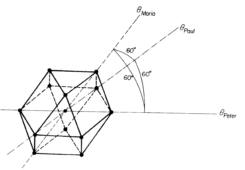
For the purpose of elucidating the symmetries of the hexagonal identification lattice, it is useful to introduce an extra (superfluous) coordinate $\theta_{4}$. First let us rewrite $S_{\Box\;Manton}$ in (244) as

$$\vec{\theta}^{T}{\bf g}\vec{\theta}=\vec{\theta}^{T}\left\{\frac{\beta}{2}\left(\left(\begin{array}[]{ccc}1/2&0&0\\ 0&1/2&0\\ 0&0&1/2\end{array}\right)+\frac{1}{2}\left(\begin{array}[]{ccc}1&1&1\\ 1&1&1\\ 1&1&1\end{array}\right)\right)\right\}\vec{\theta}=$$ (246)

$$=\frac{\beta}{4}(\theta_{1}^{2}+\theta_{2}^{2}+\theta_{3}^{2}+(\underbrace{-\theta_{1}-\theta_{2}-\theta_{3}}_{\stackrel{{\scriptstyle def}}{{=}}\theta_{4}})^{2})=\frac{\beta}{4}\sum^{4}_{i=1}\theta_{i}^{2}$$

where $\theta_{1}=\theta_{Peter},\cdots,\theta_{3}=\theta_{Maria};\theta_{4}=-\sum_{i=1}^{3}\theta_{i}$.

In this coordinate system with the superfluous coordinate $\theta_{4}$, we have the constraint

$$\sum_{i=1}^{4}\theta_{i}=0$$ (247)

and the hexagonal lattice is characterised as the set of points with coordinates

$$(\theta_{1},\theta_{2},\theta_{3},\theta_{4})\in 2\pi{\bf Z}^{4}.$$ (248)

In this notation, it is apparent that the symmetry group for the lattice and the metric consists of the permutations combined with or without a simultaneous sign shift of all four coordinates.

Each of the 12 nearest neighbours to any site of the identification lattice (e.g. the group identity) have, in the 4-tuple coordinate notation, just two non-vanishing coordinates (that sum to zero). The 1-dimensional subgroups correspond to the 6 co-linear pairs of these 12 nearest neighbours.

The 2-dimensional subgroups are of two types. One type, of which there are 4, are spanned by the identity and any (non-co-linear) pair of the 12 nearest neighbour sites that have a common non-vanishing coordinate. A given subgroup of this type contains 6 nearest neighbour sites positioned at the corners of a hexagon; all 6 such sites of a given 2-dimensional subgroup of this type have a vanishing coordinate in common; e.g., the 6 nearest neighbours with a “0” for the first coordinate belong to the same 2-dimensional subgroup of this type. That there are four such subgroups follows from the fact that there are 4 possibilities for having a common vanishing coordinate in the 4-tuple notation. The other type of 2-dimensional subgroups - there are 3 mutually orthogonal such subgroups - are each spanned by 2 pairs of nearest neighbour sites where the two sites of each such pair have no common non-vanishing coordinates. There are 3 such pairs:

$$\begin{array}[]{c}(\pm 2\pi,0,\mp 2\pi,0)\\ (0,\pm 2\pi,0,\mp 2\pi)\end{array}$$ (249)

$$\begin{array}[]{c}(\pm 2\pi,\mp 2\pi,0,0)\\ (0,0,\pm 2\pi,\mp 2\pi)\end{array}$$ (250)

$$\begin{array}[]{c}(\pm 2\pi,0,0,\mp 2\pi)\\ (0,\pm 2\pi,\mp 2\pi,0).\end{array}$$ (251)

Any of the 3 pairs (249), (250), (251) span one of the $\left(\begin{array}[]{c}3\\ 2\end{array}\right)=3$ orthogonal 2-dimensional subgroups.

The 3-dimensional “subgroup” (which of course is the whole $\mbox{\bf{R}}^{3}$ space) corresponds in the 4-tuple notation to the (whole) hyper-plane specified by

$$\{\vec{\theta}|\sum_{i=1}^{4}\theta_{i}=0\}.$$ (252)

The 0-dimensional subgroup corresponds simply to the identification lattice site that is chosen as the group identity.

7.3.2 Group volume approximation

In this approximation, which is an alternative to the monopole approximation, we calculate the free energy as a function of the couplings for each phase ansatz (i.e. each partially confining phase). The criterion for having a phase in contact with the multiple point is that there is some region of plaquette action parameter space infinitesimally close to the multiple point where the corresponding free energy function is the most stable (i.e., larger than the free energy functions of all the other phases that meet at the multiple point). In Section 6.3, the approximate expression (137) for the free energy was derived per active link. We use the notation $\log Z_{H\triangleleft G}$ for the free energy function corresponding to the phase for which $H$ is the largest confined invariant subgroup of the gauge group $G$:

$$(\log Z_{H\triangleleft G})_{\mbox{\tiny per active link}}=\log\left[\frac{(\pi/6)^{\frac{d_{G}}{2}}}{{\bf\beta}_{G}^{\frac{d_{G}}{2}}vol(G)}\right]+\log\left[\frac{(6\pi)^{\frac{d_{H}}{2}}}{{\bf\beta}_{H}^{\frac{d_{H}}{2}}vol(H)}\right].$$ (253)

where

$${\bf\beta}_{H}^{\frac{1}{2}dim\;H}\stackrel{{\scriptstyle def}}{{=}}\prod_{i}\beta_{i}^{\frac{1}{2}dim\;H_{i}}$$ (254)

and the index $i$ runs over the Lie algebra ideals of $H$.

Consider two partially confining phases in the case that one of these is confined w.r.t to the invariant subgroup $H_{I}$ and the other is confined w.r.t. the invariant subgroup $H_{J}$. At any point in parameter space where these two partially confining phases meet (including the multiple point of course) the condition to be satisfied is $\log Z_{H_{I}\triangleleft G}=\log Z_{H_{J}\triangleleft G}$. This together with (253) leads to the following condition that is fulfilled at any point on the phase boundary separating these two phases:

$$\log(6\pi)^{\frac{dim(H_{J})-dim(H_{I})}{2}}=\log\frac{{\bf\beta}_{H_{J}}^{\frac{dim(H_{J})}{2}}vol(H_{J})}{{\bf\beta}_{H_{I}}^{\frac{dim(H_{I})}{2}}vol(H_{I})}.$$ (255)

We want of course to consider (253) in the special case for which $G=U(1)^{3}$.

Using here a slightly different notation, designate by $\log Z_{H_{n}}$ the free energy per active link for the phase ansatz for which one of the above-mentioned n-dimensional subgroups $H_{n}$ of $U(1)^{3}$ ($dim(H_{n})=n$; $n\in\{0,1,2,3\}$), is confining and the factor group $U(1)^{3}/H_{n}$ behaves in a Coulomb-like way ($H_{n}$ could be one of the 1-dimensional subgroups: e.g., $H_{1}=U(1)_{Peter}$ say). Let us denote by $a$ the lattice constant of the identification lattice. Rewriting (253) and specialising to the case of the gauge group $G=U(1)^{3}$ and $H_{J}=H_{n}$ reveals the dependence of the free energy per active link on the quantity log$a$:

$$\log Z_{H_{n}}=C-(dim(U(1)^{3})+dim(H_{n}))\log a$$ (256)

where $dim(U(1)^{3})=3$ and $dim(H_{n})$ are respectively the dimension of the gauge group (i.e., the $U(1)^{3}$ part of $SMG^{3}$) and the dimension of the subgroup $H_{n}$ and $C$ is a quantity that does not depend on the identification lattice constant $a$. The slope of the various phase ansätze is just

$$\frac{d\log Z_{H_{n}}}{d\log a}=-(dim(U(1)^{3})+dim(H_{n})).$$ (257)

Upon rewriting (255), one obtains for the condition defining the phase boundary between the phase with confinement along the subgroup $H_{n}$ and the phase with confinement along $H_{m}$ the equation

$$(6\pi)^{(dim(H_{n})-dim(H_{m}))/2}=\frac{(\frac{a^{2}}{2\pi^{2}})^{dim(H_{n})/2}c_{n}(2\pi)^{dim(H_{n})}}{(\frac{a^{2}}{2\pi^{2}})^{dim(H_{m})/2}c_{m}(2\pi)^{dim(H_{m})}}\;\;(n,m\in\{0,1,2,3\})$$ (258)

where the volume $vol(H_{n})$ of the subgroup $H_{n}\subseteq U(1)^{3}$, measured in the coordinate $\theta$, is

$$vol(H_{n})=c_{n}(2\pi)^{dim(H_{n})}.$$ (259)

The quantity $c_{n}$ is a factor associated with the subgroup $H_{n}$ that depends on the geometry of the identification lattice.

As an example, consider first a cubic identification lattice (actually we shall end up using an hexagonal lattice as this better satisfies the principle of multiple point criticality). For the cubic lattice with $a=a_{1\;crit}\stackrel{{\scriptstyle def}}{{=}}2\pi\sqrt{\frac{\beta_{crit}}{2}}$, it is possible to have the confluence of three phases of the type corresponding to 1-dimensional subgroups of $U(1)^{3}$ at a multiple point - namely those corresponding to the 1-dimensional subgroups along the $Peter$, $Paul$, and $Maria$ directions of the lattice having $a_{1\;crit}=2\pi\sqrt{\frac{\beta_{crit}}{2}}$ (the subscript “1” on $a_{1\;crit}$ denotes that it is a one dimensional subgroup that is critical). Furthermore, in the case of the cubic identification lattice, it will be seen that phases corresponding to all subgroups of $G=U(1)^{3}$ are simultaneously critical when the identification lattice constant $a=a_{1\;crit}=2\pi\sqrt{\frac{\beta_{crit}}{2}}$. This follows by observing that the free energy $\log Z_{n}$ ($n\in\{0,1,2,3\}$) for the different ansätze (i.e., confinement along the various possible subgroups) are equal for the same value of the identification lattice constant $a$ (i.e., for $a=a_{1\;crit}$) because the constants $c_{n}$ in (258) are independent of the dimension $dim(H_{n})$ of the subgroup (and therefore equal). Hence the condition (258) that defines the boundary between two partially confining phases is independent of dimension. This then means that for the unit cell of the cubic identification lattice, all the quantities $\log Z_{n}$ ($n\in\{0,1,2,3\}$) intersect for $a=a_{1\;crit}=2\pi\sqrt{\frac{\beta_{crit}}{2}}=2\pi\sqrt{\frac{1.01}{2}}=4.465$. So the use of the cubic identification lattice with $a=a_{1\;crit}$ shows that it is possible to have a multiple point at which 8 partially confining phases are in contact: there is one totally confining phase (corresponding to $H_{3}$), three phases corresponding to three 2-dimensional subgroups $H_{2}$, three phases corresponding to three 1-dimensional subgroups $H_{1}$, and a totally Coulomb-like phase corresponding to $H_{0}$. In particular, the coupling corresponding to the diagonal subgroup of $U(1)^{3}$ (in the first approximation, this is the coupling that we identify with the continuum $U(1)$ coupling) is down by a factor $\sqrt{3}$ relative to the critical coupling for a $U(1)$ lattice gauge theory. This follows because the inverse of the ratio of the length of the diagonal to the critical lattice constant is $\sqrt{3}$. Phenomenologically, a factor of roughly $\sqrt{6}$ rather than $\sqrt{3}$ is needed so we must conclude that for the $U(1)$ continuum coupling, the prediction of the multiple point criticality principle using a cubic identification lattice is at odds with experiment.

However, the multiple point criticality principle states that we should seek the values of the continuum $U(1)$ coupling at a point in parameter space at which a maximum number of phases come together. We have already seen that for a hexagonal identification lattice in the covering group $\mbox{\bf{R}}^{3}$ of the gauge group $U(1)^{3}$, we can, in terms of the 12 nearest neighbours of a site in the hexagonal identification lattice, identify a total of 15 subgroups corresponding to 15 partially confining phases. Even though we shall discover in the sequel that 3 of these 15 partially confining phases - the 2-dimensional “orthogonal” phases given by (249-251) - are not realistically realizable in the volume approximation inasmuch as these phases are “pushed” too far away from the multiple point in the volume approximation, there remains 12 partially confining phases that can be made to convene at the multiple point. This is, in view of the multiple point criticality principle, an improvement upon the total of 8 phases that can be realized at the multiple point in the case of the cubic identification lattice.

It will be seen that the price we must pay for realizing these 12 remaining partially confining phases at the multiple point in the case of the hexagonal identification lattice instead of the 8 partially confining phases of the cubic identification lattice is that these 12 phases no longer come together exactly at a common value of the identification lattice constant $a$ if we use a pure Manton action (232).

For the hexagonal identification lattice, the problem is that when the lattice constant $a$ is chosen so that $a=a_{1\;crit}\stackrel{{\scriptstyle def}}{{=}}2\pi\sqrt{\frac{\beta_{crit}}{2}}$ corresponding to criticality for the 1-dimensional subgroups, this choice fixes the values of the couplings for the 2- and 3-dimensional subgroups at sub-critical values. For example, for $a=a_{1\;crit}$, the free energy functions $\log Z_{0}$ and $\log Z_{1}$ are equal corresponding to the coexistence of the totally Coulomb-like phase and the six phases that are confined along 1-dimensional subgroups. However, if for example one wishes to have coexistence of the totally Coulomb-like phase and the four phases that are confined along the four 2-dimensional subgroups, it will be seen (Table 7) that $\log a$ must be decreased by $\frac{1}{4}\log(4/3)$. But this reduction in $\log a$ would put the phases corresponding to 1-dimensional subgroups into confinement.

Information about the cubic and hexagonal lattices are tabulated in Tables 6 and 7. Table  6 pertains to the cubic lattice; Table  7 to the hexagonal identification lattice. The entries in the first four (five) rows and columns of Table 6 (Table 7) give the values of the identification lattice constant $a^{2}$ (in terms of $a^{2}_{1\;crit}$) at which pairs (corresponding to a row and column heading) of free energy phase ansätze intersect; i.e., these entries are the quantities

$$\frac{a^{2}}{a^{2}_{1\;crit}}=\left(\frac{c_{n}}{c_{m}}\right)^{\frac{-2}{dim(H_{n})-dim(H_{m})}}\;\;\;\;(n,m\in\{0,1,2,3\})$$ (260)

obtained by rewriting (258) and using that $a_{1\;crit}^{2}=3\pi$ (obtained from (258) with $n=1$ and $m=0$. The quantities $a$ and $a_{1,\;crit}=2\pi\sqrt{\frac{\beta_{crit}}{2}}$ are respectively the identification lattice constant and the critical value of the (identification) lattice constant. The quantities $c_{n}$ are the volume correction factors associated with the subgroup $H_{n}$ ($n\in\{0,1,2,3\}$). These are also tabulated in the tables below. All the volume correction factors are unity for the cubic identification lattice. For the hexagonal lattice, $c_{0}$ and $c_{1}$ are both unity whereas $c_{2}=\sqrt{3/4}$ and $c_{3}=\sqrt{1/2}$ corresponding respectively to the ratio of area of a minimal parallelogram in the hexagonal lattice to the area of a simple plaquette in the cubic lattice and the ratio of the volume of a (minimal) parallelpipidum of the hexagonal lattice to the volume of a simple cube in the cubic lattice.

Table 6: Parameters pertaining to the cubic identification lattice. The entries in the first four rows and columns are all unity because phases corresponding to all subgroups convene at the multiple point for the critical value of the coefficient $\frac{1}{e^{2}_{U(1)\;crit}}$ in the Manton action; i.e., the quantity $\frac{a^{2}}{a^{2}_{1\;crit}}=\left(\frac{c_{n}}{c_{m}}\right)^{\frac{-2}{dim(H_{n})-dim(H_{m})}}$ $(n,m\in\{0,1,2,3\})$ is unity for all $m,n\in\{0,1,2,3\}$. The quantities in the last three columns are as explained in Table (7).

CUBIC	$\log Z_{H_{0}}$	$\log Z_{H_{1}}$	$\log Z_{H_{2}}$	$\log Z_{H_{3}}$	$\frac{d\log Z_{H_{n}}}{d\log a}$	# phases	$c_{n}$
$\log Z_{H_{0}}$	1	1	1	1	-3	1	1
$\log Z_{H_{1}}$		1	1	1	-4	3	1
$\log Z_{H_{2}}$			1	1	-5	3	1
$\log Z_{H_{3}}$				1	-6	1	1

Table 7: Parameters pertaining to the hexagonal identification lattice. As regards the five rows and first five columns, the entry in the n$th$ column and the m$th$ row is the coefficient $\frac{a^{2}}{a^{2}_{1\;crit}}=\left(\frac{c_{n}}{c_{m}}\right)^{\frac{-2}{dim(H_{n})-dim(H_{m})}}$ $(n,m\in\{0,1,2,3\})$ . This is the quantity by which $\frac{1}{e^{2}_{U(1)\;crit}}$ must be multiplied in order that the phases confined w.r.t. the $n$-dimensional and $m$-dimensional subgroups can come together at the multiple point. The slope of the $\frac{d\log Z_{H_{m}}}{d\log a}$, calculated from (257), is given in the sixth column. Column seven gives the number of phases of dimension $m$. The entries in column eight are the “volume” correction factors $c_{n}$ (see (259)) in the hexagonal lattice relative to the corresponding (unit) “volumes” in the cubic lattice.

HEXAG.	$\log Z_{H_{0}}$	$\log Z_{H_{1}}$	$\log Z_{H_{2}orthog}$	$\log Z_{H_{2}}$	$\log Z_{H_{3}}$	$\frac{d\log Z_{H_{n}}}{d\log a}$	# phases	$c_{n}$
$\log Z_{H_{0}}$	1	1	1	$\sqrt{\frac{4}{3}}$	$\sqrt[3]{2}$	-3	1	1
$\log Z_{H_{1}}$		1	1	$\frac{4}{3}$	$\sqrt{2}$	-4	6	1
$\log Z_{H_{2}orthog}$			1		2	-5	3	1
$\log Z_{H_{2}}$				1	$\frac{3}{2}$	-5	4	$\sqrt{\frac{3}{4}}$
$\log Z_{H_{3}}$					1	-6	1	$\sqrt{\frac{1}{2}}$

However, the amount by which the free energy functions for these different phases fail to intersect at a common value of the identification lattice is hopefully small enough to be dealt with meaningfully by perturbing the Manton action (using 4$th$ and 6$th$ order terms) in such a way as to allow 12 phases to convene at a multiple point.

We therefore replace the Manton action (containing by definition only second order terms) by a more complicated action:

$$S_{\Box,\;Manton}\rightarrow S_{\Box,\;Manton}+S_{\Box,\;h.o.}$$

where $S_{\Box,\;h.o.}$ designates higher than second order terms. In choosing the higher order terms, we want to use the lowest possible order terms that bring together the desired phases at the multiple point.

The number of additional terms needed depends on how many phases we want to bring together at the multiple point. As explained above, we have decided to settle for the 12 phases (corresponding to one 0-dimensional, six 1-dimensional, four 2-dimensional, and one 3-dimensional subgroups) that have the smallest possible volume on the hexagonal lattice and which are not too far from being able to convene at the multiple point with the Manton action alone. These 12 phases seem to exhaust the ones for which a modification of the couplings using the procedure to be explained below can be regarded as a small perturbation; for example, the diagonal subgroup coupling (with pure Manton action) is so far removed from the critical couplings of the 12 hexagonal lattice phase discussed above that we a priori give up trying to have a phase confined along the diagonal subgroup in contact with the multiple point. The same applies presumably to the 2-dimensional “orthogonal” subgroups (249-251) as already mentioned above.

Due to the high degree of symmetry of the hexagonal lattice, the conditions for the criticality are identical for phases corresponding to the four 2-dimensional subgroups and the six 1-dimensional subgroups. So the number of parameters we need to get all 12 phases to convene is effectively that for four phases (corresponding to the four possible dimensionalities of subgroups). This requires 4-1=3 parameters. This can be compared to the generic number of parameters necessary for the meeting of 12 phases: 12-1=11 parameters. The point is that the symmetry of the hexagonal identification lattice allows a non-generic multiple point in an action parameter space spanned by just three parameters. These can be chosen as the Manton parameter (i.e., the coefficient to the second order term in a Taylor expansion of the action) and two parameters that are coefficients to respectively a 4th and a 6th order term. These 4th and 6th order terms are to be chosen so as to have the same symmetry as the hexagonal lattice; otherwise we lose the symmetry that allows a non-generic multiple point. Without the symmetry, we would in general need 11 parameters instead of 3. It is also necessary that these two terms contribute differently to the different free energy functions for the different types of subgroup that we want to bring to the multiple point. Otherwise we could compensate for the effect of these higher order terms for all subgroups by using a single new effective coefficient to the Manton term. In other words, we want our high order terms to be such that these give different new effective coefficients to the second order action term for different subgroups. The effective second order coefficient is defined as the coefficient in the Manton action that would give the same fluctuation width inside the subgroup in question as there would be with the higher order terms in place. To this end we use linear combinations of spherical harmonics $Y_{lm}$ with $l=4$ and $l=6$ that have the same symmetry as the cub-octahedron (which can be taken as the “unit cell” of the hexagonal identification lattice). These linear combinations, denoted $Y_{4\;comb}$ and $Y_{6\;comb}$, are invariant under the symmetry of the cub-octahedron.

In using the $Y_{4\;comb}$ and $Y_{6\;comb}$ as perturbations to the Manton action, we obtain an effective Manton inverse squared coupling strength that varies with the direction $\vec{\xi}$:

$$\frac{1}{e^{2}_{eff}(\vec{\xi})}.$$ (261)

Here $\vec{\xi}$ denotes a vector in $\mbox{\bf{R}}^{3}$ (the covering space of $U(1)^{3}$).

The desired combinations $Y_{4\;comb}$ and $Y_{6\;comb}$ that have the symmetry of the cub-octahedron turn out, after a rather strenuous calculation, to be

$$Y_{4\;comb}=\frac{2}{3}\sqrt{7}Y_{40}+\frac{4}{3}\sqrt{5}(Y_{43}+Y_{4,-3})/i\sqrt{2}$$ (262)

and

$$Y_{6\;comb}=(-4\sqrt{\frac{3}{35}})Y_{60}+\sqrt{\frac{11}{10}}(Y_{66}+Y_{6,-6})/\sqrt{2}+(Y_{63}+Y_{6,-3})/i\sqrt{2}.$$ (263)

These have been calculated in a coordinate system in which the $z$-axis coincides with a 3-axis of symmetry of the cub-octahedron. In Table 8 these combinations $Y_{4\;comb}$ and $Y_{6\;comb}$ are averaged over the 1,2 and 3-dimensional subgroups of $U(1)^{3}$. The fact that both combinations vanish for $U(1)^{3}$ (the 3-dimensional subgroup) reflects of course the property that spherical harmonics vanish when integrated over the surface of a sphere. Table 8 also gives the values of $Y_{4\;comb}$ and $Y_{6\;comb}$ along the diagonal subgroup of $U(1)^{3}$.

Table 8: The $4th$ and $6th$ order action contributions needed to realize 12 partially confining phases at the multiple point. The contributions have the symmetry of the hexagonal identification lattice.

$$\begin{array}[]{|c|c|c|}\hline\cr\mbox{subgroup}&Y_{4\;\;comb}&Y_{6\;\;comb}\\ \hline\cr\langle Y_{l\in\{4,6\}}\rangle_{3-dim}&0&0\\ \hline\cr\langle Y_{l\in\{4,6\}}\rangle_{2-dim}&\frac{\sqrt{7}}{4}&\frac{5}{4}\sqrt{\frac{3}{35}}\\ \hline\cr Y_{l\in\{4,6\};\;1-dim}&\frac{\sqrt{7}}{4}&\frac{117}{32}\sqrt{\frac{3}{35}}\\ \hline\cr Y_{l\in\{4,6\};\;diagsubgr}&\frac{2\sqrt{7}}{3}&-4\sqrt{\frac{3}{35}}\\ \hline\cr\end{array}$$ (264)

Figure 21: Contours of constant perturbed Manton action for $U(1)^{2}$ represented in the covering group $\mbox{\bf{R}}^{2}$ with the metric in the plane of the paper that is identified with the Manton action metric. The hexagonal lattice of “$\bullet$” are points identified in compactifying from $\mbox{\bf{R}}^{2}$ to $U(1)^{2}$. The purpose of the correction - it is sixth order and gives the contours a “webbed feet” look - is to increase $\log Z$ for the phases with confinement along one of the three 1-dimensional subgroups - i.e., along the $\theta_{Peter}$ axis, the $\theta_{Paul}$ axis and along the line given by $\theta_{Peter}+\theta_{Paul}=0$ - while disfavouring fluctuations along directions that bisect the angles between these 1-dimensional subgroup directions. This is accomplished by decreasing the gradient of the action in these three subgroup directions while increasing the gradient in directions that bisect the above-mentioned three subgroups

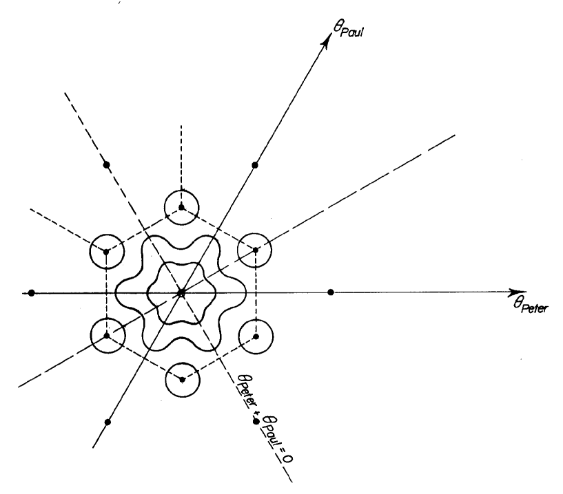
Using the Tables 6, 7, and 8, let us now determine the coefficients to the 2$nd$ order (i.e. Manton) as well as 4$th$ and 6$th$ order action terms by using the requirement that averages over the 1, 2 and 3-dimensional subgroups of $U(1)^{3}$ are equal to the $U(1)$ critical inverse squared coupling $1/e^{2}_{U(1)\;crit}$ when the volume correction factors for the hexagonal lattice are taken into consideration. These latter are given by (260). Using that $\beta=1/e^{2}=a^{2}/2\pi^{2}$ we can write the condition to be satisfied if the average over the subgroup $H_{n}$ - i.e., $\langle 1/e^{2}(\vec{\xi})\rangle_{H_{n}}$ - is to have a value corresponding to the boundary between a phase confined along $H_{n}$ and the totally Coulomb phase:

$$\langle\frac{1}{e^{2}(\vec{\xi})}\rangle_{H_{n}}=\left(\frac{c_{n}}{c_{0}}\right)^{\frac{-2}{dim(H_{n})-dim(H_{0})}}\frac{1}{e^{2}_{U(1)\;crit}}$$ (265)

where $c_{0}$ and $H_{0}$ correspond to the totally Coulomb phase. Eqn. (265) yields three equations - one for each type of subgroup $H_{n}$ ($n=dim(H_{n})$).

For $n=3$ there are no contributions to $\langle\frac{1}{e^{2}_{eff}(\vec{\xi})}\rangle_{3-dim\;subgr}$ from $Y_{4\;comb}$ and $Y_{6\;comb}$. The second order coefficient $\frac{1}{e_{Manton}^{2}}$ is therefore determined by the one equation

$$\langle\frac{1}{e^{2}_{eff}(\vec{\xi})}\rangle_{3-dim\;subgr}=\frac{1}{e_{Manton}^{2}}=\left(\frac{c_{3}}{c_{0}}\right)^{\frac{-2}{3-0}}\frac{1}{e^{2}_{U(1)\;crit}}=2^{\frac{1}{3}}\frac{1}{e^{2}_{U(1)\;crit}}.$$ (266)

The coefficients to $Y_{4\;comb}$ and $Y_{6\;comb}$ - denoted respectively as $B_{4}$ and $B_{6}$ - can be obtained from the equations for $\langle\frac{1}{e^{2}_{eff}(\vec{\xi})}\rangle_{1-dim\;subgr}$ and $\langle\frac{1}{e^{2}_{eff}(\vec{\xi})}\rangle_{2-dim\;subgr}$. Assigning dimensionality to the strictly speaking dimensionless quantity $1/e^{2}$, we use that [$B_{4}$]=[$\frac{1}{e^{4}}$] and [$B_{6}$]=[$\frac{1}{e^{6}}$].

For $n=1$ we have:

$$\langle\frac{1}{e^{2}_{eff}(\vec{\xi})}\rangle_{1-dim\;subgr}^{3}=B_{6}\langle Y_{6\;comb}\rangle_{1-dim\;subgr}+\left(\frac{1}{e^{4}_{Manton}}+B_{4}\langle Y_{4\;comb}\rangle_{1-dim\;subgr}\right)^{\frac{3}{2}}=$$ (267)

$$=B_{6}\frac{117}{32}\sqrt{\frac{3}{35}}+\left(\frac{2^{\frac{2}{3}}}{e^{4}_{U(1)\;crit}}+B_{4}\frac{\sqrt{7}}{4}\right)^{\frac{3}{2}}=\left(\left(\frac{c_{1}}{c_{0}}\right)^{\frac{-2}{3-0}}\frac{1}{e^{2}_{U(1)\;crit}}\right)^{3}=\left(1\frac{1}{e^{2}_{U(1)\;crit}}\right)^{3}.$$

For $n=2$ we have:

$$\langle\frac{1}{e^{2}_{eff}(\vec{\xi})}\rangle_{2-dim\;subgr}^{3}=B_{6}\langle Y_{6\;comb}\rangle_{2-dim\;subgr}+\left(\frac{1}{e^{4}_{Manton}}+B_{4}\langle Y_{4\;comb}\rangle_{2-dim\;subgr}\right)^{\frac{3}{2}}=$$ (268)

$$=B_{6}\frac{5}{4}\sqrt{\frac{3}{35}}+\left(\frac{2^{\frac{2}{3}}}{e^{4}_{U(1)\;crit}}+B_{4}\frac{\sqrt{7}}{4}\right)^{\frac{3}{2}}=\left(\left(\frac{c_{2}}{c_{0}}\right)^{\frac{-2}{2-0}}\frac{1}{e^{2}_{U(1)\;crit}}\right)^{3}=\left(\sqrt{\frac{4}{3}}\frac{1}{e^{2}_{U(1)\;crit}}\right)^{3}.$$

The values of the geometric factors $c_{n}$ are from Table 7 and the values of $\langle Y_{6\;comb}\rangle_{n-dim\;subgr\;H_{n}}$ and $\langle Y_{4\;comb}\rangle_{n-dim\;subgr\;H_{n}}$ $(n=dim(H_{n})\in\{0,1,2,3\})$ are taken from Table 8.

Solving these equations for the coefficients $B_{4}$ and $B_{6}$ yields

$$B_{4}=-0.1463\mbox{ and }B_{6}=-0.7660$$ (269)

We have now succeeded in fitting three coefficients of a modified Manton (i.e. a plaquette action dominated by a second order “Manton” term but having perturbative 4$th$ and 6$th$ order terms) in such a way that 4 types of phases $H_{n}$ convene at a multiple point in the sense that $\langle 1/e^{2}_{eff}(\vec{\xi})\rangle_{H_{n}}$ ($n=dim(H_{n})\in\{0,1,2,3\}$) is equal to the $U(1)$ critical coupling up to a factor pertaining to the geometry of the hexagonal identification lattice. Because the modified Manton action has the symmetry of the hexagonal lattice, multiple point criticality for a phase corresponding to a given dimension implies multiple point criticality for all phases corresponding to a given dimension. For this reason we achieve multiple point criticality for a total of 12 phases. The averaging $\langle 1/e^{2}_{eff}(\vec{\xi})\rangle_{H_{n}}$ can be taken as an average over all directions within the subgroup $H_{n}$ using a measure defined by being invariant under rotations leaving the Manton metric invariant.

So we now have at our disposal a means of calculating a directionally dependent effective inverse squared coupling where the directional dependence comes from the perturbative $4th$ and $6th$ order action terms. In a later section, we shall want to calculate $1/e^{2}_{eff}$ in the direction corresponding to the diagonal subgroup (in a chosen coordinate system).

Having now developed some tools for constructing approximate phase diagrams for the gauge group $U(1)^{3}$ in which the (or some chosen) multiple point can be sought out, we proceed to do calculations in the next Section (Section 8).

theu1d.tex 31 May 96 sent

8 Calculation of the numerical value of the continuum coupling

8.1 Outline of procedure

The aim now is to calculate the continuum $U(1)$ standard model weak hyper-charge coupling corresponding to the “diagonal subgroup” coupling at the multiple point of the $AGUT$ gauge group $SMG^{3}$. In principle, the multiple point should be sought in a very high dimensional action parameter space that is also in contact with a multitude of phases that are alone confined w.r.t discrete $\mbox{\bf{Z}}_{N}$ subgroups. In an even more correct search for the multiple point involving phases with confining discrete subgroups, we should really consider Abelian and non-Abelian groups at the same time (i.e, the full $SMG^{3}$ or perhaps an even larger group) because discrete subgroups having the characteristic of being non-factorizable could a priori simultaneously involve Abelian subgroups and centres of semi-simple subgroups.

Figure 22: The phase diagram for $U(1)$ when the two-parameter action is used. This type of action makes it possible to provoke the confinement of $\mbox{\bf{Z}}_{2}$ (or $\mbox{\bf{Z}}_{3}$) alone.

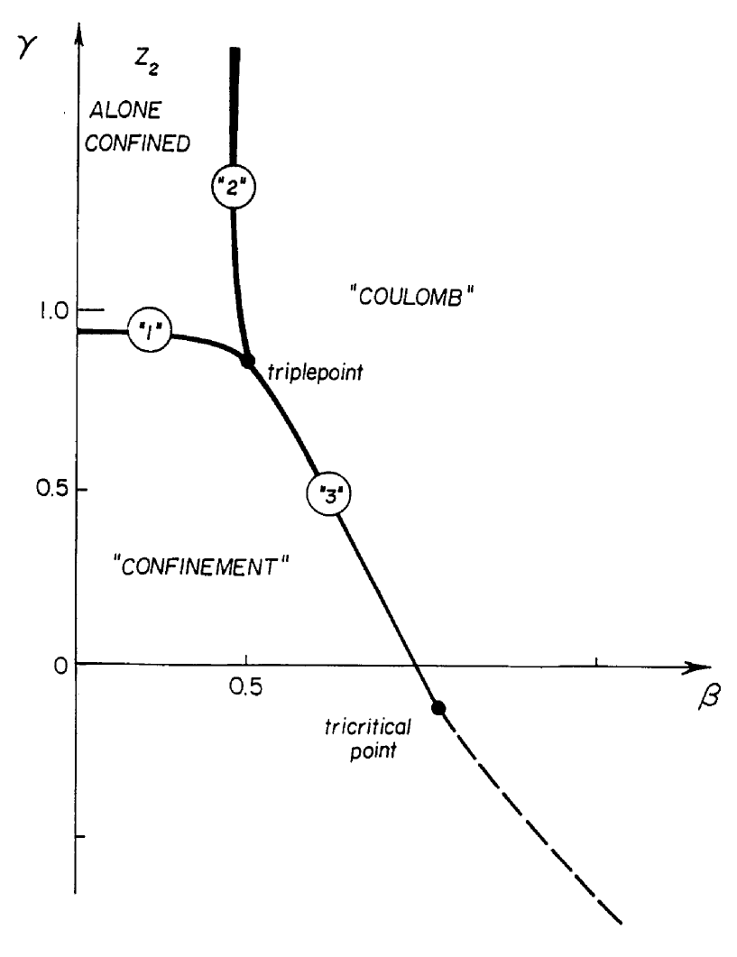
As a crude prototype to a $U(1)^{3}$ phase diagram, we consider the (generic) phase diagram spanned by the parameters of an action with $\cos\theta,\cos\frac{\theta}{2}$ and $\cos\frac{\theta}{3}$ terms. This action, which is one of the simplest generalisations of the pure Wilson action, has been studied extensively[72] and many features of the phase diagram (Figure 22) are well understood. From the triple point (TP) (which is the “multiple point” in this 2-dimensional phase diagram) emanate three characteristic phase borders: the phase border “3” separates the totally confining and totally Coulomb-like phases; the phase border “1” separates the totally confining phase from the phase where only the discrete subgroup $\mbox{\bf{Z}}_{2}$ is confined; this latter phase is separated from the totally Coulomb-like phase by the phase border “2”.

The calculational procedure to be used in determining the continuum $U(1)$ coupling is approximative and is done in two steps:

1. first we calculate the factor analogous to the factor $3=N_{gen}$ in the non-Abelian case; we call this the enhancement factor and denote it as $\frac{1/\alpha_{U(1)^{3}\;diag}}{1/\alpha_{U(1)_{crit\;TP}}}$. This factor lies in the range 6.0 - 8.0 depending on the degree of “first-orderness” of the triple point (TP) transition at boundary “2”.

2. In the second step, the continuum $U(1)$ coupling corresponding to the multiple point value for a single $U(1)$ is determined using an analogy to a procedure proposed by Luck[82] and developed by Jersàk[83].

This two-step calculation can be done using more or less good approximations as regards the extent to which the continuum $U(1)$ coupling value reflects having phases solely confining w.r.t. discrete subgroups among the phases that convene at the multiple point. Let us outline the possible approximations in the order of increasing goodness.

1. The roughest calculation would be to use a single parameter action with hexagonal symmetry without regard to having phases at the triple point (TP) that are confining solely w.r.t. the discrete subgroups $\mbox{\bf{Z}}_{2}$ and $\mbox{\bf{Z}}_{3}$ of $U(1)^{3}$. In this approximation, these discrete subgroups are treated as though they were totally confining inasmuch as it is a $U(1)$-isomorphic factor group obtained essentially by dividing $\mbox{\bf{Z}}_{2}\times\mbox{\bf{Z}}_{3}$ out of the $U(1)$ centre of $SMG$ that is identified with the lattice $U(1)$ critical coupling.

2. By using a two-parameter action (later a three parameter action) leading to the phase diagram of Figure 22, the action now acquires a (nontrivial) dependence on the elements within the cosets of the factor group $U(1)/\mbox{\bf{Z}}_{2}$ (or the factor group $U(1)/(\mbox{\bf{Z}}_{2}\times\mbox{\bf{Z}}_{3})$ in the case of a three-parameter action) that can reveal how close the discrete subgroups are to being critical. However these details are of little importance to the $U(1)$ continuum coupling; the latter depends essentially only on a single yet to be defined parameter $\gamma_{eff}$ the critical value of which is very nearly constant along the phase boundary “1” of Figure 22. Hence the $U(1)$ continuum coupling is also approximately constant along this phase boundary in accord with the rule described in the footnote on page 226. The critical value $\gamma_{eff\;crit}$ of the parameter $\gamma_{eff}$ is expressible in terms of the critical lattice parameters available from computer data for a lattice gauge theory with a single $U(1)$.

3. The effect on the continuum coupling of having phases convening at the multiple point that are confined solely w.r.t. $\mbox{\bf{Z}}_{2}$ and solely w.r.t. $\mbox{\bf{Z}}_{3}$ appears first when we take into account the discontinuity in $\Delta\gamma_{eff}$ encountered in crossing the boundary “2” at the multiple point. As we in both steps A. and B. above want to use the value of $\gamma_{eff}$ corresponding to the totally Coulomb-like phase at the multiple point, it is important for our calculation of the $U(1)$ continuum coupling to take the “jump” $\Delta\gamma_{eff}$ into account. Inasmuch as the continuum subgroup degrees of freedom are in the same phase on both sides of boundary “2”, this discontinuity $\Delta\gamma_{eff}$ is entirely due to a phase transition for the discrete subgroup(s). Moreover, the presence of a discontinuity presumably reflects the degree of first-orderness of the triple point transition at border “2” inherited from a pure $\mbox{\bf{Z}}_{2}$ and $\mbox{\bf{Z}}_{3}$ transition (i.e., for $\gamma>>1$ in Figure 22).

4. The discrete subgroups $\mbox{\bf{Z}}_{2}$ and $\mbox{\bf{Z}}_{3}$ contribute differently to the “jump” $\Delta\gamma_{eff}$ in crossing the boundary “2” due to the fact that $\mbox{\bf{Z}}_{2}^{3}$ does not inherit the hexagonal symmetry of $U(1)^{3}$ while $\mbox{\bf{Z}}_{3}^{3}$ is more likely to do so. This is discussed at the end of Section 7.2.

It is important to recall that the normalisation of the $U(1)$ that we have argued for is implemented by the identification of the $U(1)$ lattice critical coupling with the ($U(1)$-isomorphic) factor-group $=SMG/(SU(2)\times SU(3))$ for some one of the Cartesian product factors say $SMG_{Peter}$. Since we have argued or assumed that phases with genuine discrete subgroups of this $U(1)$ factor-group are not to be in contact with the multiple point chosen by Nature, the only discrete subgroups that are to be taken into account are discrete subgroups of the $U(1)$ subgroup of $SMG$. The relation between the $U(1)$ subgroup and the factor-group $SMG/(SU(2)\times SU(3))$ can be described as $U(1)_{factorgr}=U(1)_{subgr}/{\bf Z}_{6}$.

In using $U(1)/\mbox{\bf{Z}}_{6}$ as the factor group to be identified with the lattice critical $U(1)$, we identify the elements of $\mbox{\bf{Z}}_{6}$ and thereby “hide” any differences that there might be in the probabilities for being at different elements of $\mbox{\bf{Z}}_{6}$ when a one-parameter action is used (approximation 1 in list above). But the details of how the heights of the peaks in probability at different elements of $\mbox{\bf{Z}}_{6}$ differ are important if we want to arrange that the discrete subgroups of $\mbox{\bf{Z}}_{6}$ are by themselves to be confined in phases convening at the triple point. However such details become visible again if the (one-parameter) Wilson action (roughest approximation 1 in the list above) is replaced by the (two-parameter) “mixed” fundamental-adjoint action (approximation 2 and 3 in the list above). By introducing an additional parameter in this way, we render the group elements identified in the factor groups $U(1)_{subgr}/\mbox{\bf{Z}}_{2}$ and $U(1)_{subgr}/\mbox{\bf{Z}}_{3}$ inequivalent (i.e., the action acquires a dependence on the elements within the cosets of these factor groups). So in effect, by going from the Wilson action to the two-parameter action we lift the factor group up into a kind of covering space. The result is that by replacing the $U(1)_{factorgr}$ critical coupling by the triple point coupling for the $U(1)_{subgr}$ of $SMG$, we essentially arrange that the subgroups ${\bf Z}_{2}$ and ${\bf Z}_{3}$ can confine individually in phases that convene at the triple point (TP).

In both steps A. and B. of the calculation of the continuum $U(1)$ coupling, we make use of the “jump” $\Delta\gamma_{eff}$ in the quantity $\gamma_{eff}$ that in Section 8.2 below will be argued to be an effective coupling in the sense that in the region of the phase diagram near the phase border “1” in Figure 22 (i.e., on both sides of “1”) it is to a good approximation valid that the phase realized (i.e., the totally confined or the phase with only $\mbox{\bf{Z}}_{2}$ confined) is determined by the value of this one variable $\gamma_{eff}$ ($\gamma_{eff}$ is a certain combination of the parameters $\gamma$ and $\beta$ of the two-parameter action (see Figure 22)). Consequently, the variable $\gamma_{eff}$ is necessarily constant along the phase boundary “1” and we can also assume that the corresponding continuum coupling has a constant value along this boundary. The change in $\gamma_{eff}$ - i.e. $\Delta\gamma_{eff}$ - comes first at the boundary “2” in going into the totally Coulomb-like phase. The value of $\Delta\gamma_{eff}$ (calculated in Section 8.3) depends on the degree of “first-orderness” that at the multiple point ($\gamma\approx 1$) is inherited from the pure $\mbox{\bf{Z}}_{2}$ and $\mbox{\bf{Z}}_{3}$ transitions at $\gamma\rightarrow\infty$. Without the correction for discrete subgroups embodied by $\Delta\gamma_{eff}$, the multiple point coupling is obtained as if the discrete subgroups were totally confining.

In the step A., the quantity $\Delta\gamma_{eff}$, which reflects the degree of first-orderness inherited from the pure $\mbox{\bf{Z}}_{2}$ and $\mbox{\bf{Z}}_{3}$ transition in crossing boundary “2” at the multiple point, is used to interpolate between the enhancement factor of about 8 obtained with the volume approximation and the enhancement factor of 6 obtained with the independent monopole approximation. These approximations are most suitable for respectively first and second order transformations. The calculation of the enhancement factor is done in Section 8.4.

In step B. of the calculation (performed in Section 8.5), the quantity $\Delta\gamma_{eff}$ is again used - this time in the combination $\gamma_{eff}+\Delta\gamma_{eff}$ - to calculate the $U(1)$ continuum coupling corresponding to the triple point values of a (single) $U(1)$ lattice gauge theory. We seek the continuum coupling in the corner of the totally Coulomb-like phase (necessary if Planck-scale confinement of observed fermions is to be avoided) that lies at the triple point - that is, in the “corner” formed by the phase borders “2” and “3”. According to the above argumentation, we know that the continuum coupling at any position along the border “1”: it is just equal to the value at $\gamma=\gamma_{crit}$ and $\beta=0$. In particular, this is true at the multiple point in the phase with only $\mbox{\bf{Z}}_{2}$ confining (i.e., in the “corner” formed by the phase boundaries “1” and “2”). But as argued above, we want the coupling corresponding to the Coulomb phase “corner” formed by borders “2” and “3”. This requires a correction that accounts for going from the multiple point corner formed by “1” and “2” to the multiple point corner formed by borders “2” and “3” (and in principle also a small correction from crossing border “1”). It is this transition, corresponding to the transition from a phase with solely $\mbox{\bf{Z}}_{2}$ confining to a totally Coulomb-like phase that is accompanied by the “jump” denoted by $\Delta\gamma_{eff}$.

8.2 The approximation of an effective $\gamma$

In the literature ([72, 73]) we find the phase diagram for a $U(1)$ group with a mixed lattice action having a $\gamma$ term defined on the factor-group $U(1)/{\bf Z}_{2}$:

$$S_{\Box}(\theta)=\gamma cos(2\theta)+\beta cos(\theta).$$ (270)

With this action it is easy to provoke confinement of the whole group as well as the totally Coulomb phase and phase confined solely w.r.t. a discrete subgroup isomorphic to $\mbox{\bf{Z}}_{2}$ for a judicious choice of the action parameters $\gamma$ and $\beta$ that span the phase diagram in Figure 22. Indeed the phase diagram of Figure 22 clearly reveals a triple point common to three phases. The interpretation of these phases as the three referred to above is confirmed by rough mean field estimates for the phase borders. In the case of the non-Abelian subgroups $SU(2)$ and $SU(3)$, two of the phases in Figure 22 are actually connected, because one of the phase borders ends at a tri-critical point. However, this does not of course preclude the existence of a multiple (i.e., triple) point.

Before proceeding, it is useful to change notation by scaling the variable $\theta$ down by a factor two inasmuch as it is recalled (see 7.1.1) that we want to normalise relative to the factor group $U(1)/\mbox{\bf{Z}}_{2}$.

$$S_{\Box}(\theta)=\gamma\cos(\theta)+\beta\cos(\theta/2).$$ (271)

Note that with this notational convention, Bianchi identities are fulfilled modulo $4\pi$. In discussions of monopoles dealt with in later sections, we shall have occasion to distinguish “full” $4\pi$-monopoles and “minimal strength” $\frac{2\pi}{4\pi}$-monopoles. The latter will be seen to correspond to the “length” of the factor group $U(1)/\mbox{\bf{Z}}_{2}$. These remarks first become relevant and more transparent when, in a later section, we explain the idea of “minimal strength” monopoles. In the case of $\mbox{\bf{Z}}_{2}$, such monopoles are referred to as $\frac{2\pi}{4\pi}$-monopoles. These will be seen to be the monopoles present relative to a $\mbox{\bf{Z}}_{2}$ background field.

In order to obtain numerical results, the multiple point coupling in this diagram will in a later Section be related to the point at which $\beta=0,\gamma=\gamma_{critical}$ inasmuch as we have a procedure for relating this point to the continuum coupling at the triple point (hereafter “TP”) “corner” formed by the phase boundaries “1” and “2” and subsequently at the for us interesting TP “corner” formed by the phase boundaries “2” and “3” (i.e., the totally Coulomb phase at the TP - see Figure 22). We shall actually argue that to a very good approximation the continuum coupling does not vary along the phase border “1” (separating the “total confinement” and the “phase with only ${\bf Z}_{2}$ confining”) in going from $(\beta,\gamma)=(0,\gamma_{crit})$ to the corner at the TP formed by the phase boundaries “1” and “2”. It is first upon crossing the phase boundary “2” into the totally Coulomb phase at the TP that there is a change - a jump $\Delta\gamma_{eff}$ - in the quantity $\gamma_{eff}$ that immediately below will be seen to be an effective coupling. This jump $\Delta\gamma_{eff}$ comes from a jump in the relative probability of finding the plaquette variable at the(a) non-trivial element of $Z_{2}(\mbox{\bf{Z}}_{3})$ upon making the transition at boundary “2” separating the totally Coulomb-like phase from the phase solely confined w.r.t. $\mbox{\bf{Z}}_{2}$ or $\mbox{\bf{Z}}_{3}$ in Figure 22. As the continuum degrees of freedom are in the same phase on both sides of the boundary “2”, the discontinuity $\Delta\gamma_{eff}$ must be entirely due to the discrete subgroup transition which inherits a considerable degree of the first order nature of the pure (i.e., for $\gamma\rightarrow\infty$) discrete group transition.

In order to see how the effective coupling $\gamma_{eff}$ comes about, we consider the partition function for the action (271)

$$Z=\int{\cal D}\theta(\mbox{\begin{picture}(4.15,10.0)\put(0.0,3.0){\circle*{2.0}} \put(0.0,2.75){\line(1,0){7.0}} \put(7.3,3.0){\circle*{2.0}}\mbox{ } \end{picture} })\exp(\sum_{\Box}(\gamma cos(\theta)+\beta cos(\theta/2))).$$ (272)

It can be rewritten as

$$Z=\int{\cal D}\hat{\theta}(\mbox{\begin{picture}(4.15,10.0)\put(0.0,3.0){\circle*{2.0}} \put(0.0,2.75){\line(1,0){7.0}} \put(7.3,3.0){\circle*{2.0}}\mbox{ } \end{picture} })\exp(\sum_{\Box}(\gamma\cos(\hat{\theta})+\log(\cosh(\beta(\cos(\hat{\theta}/2)-1)))+\log(1+\langle\sigma\rangle_{\hat{\theta}}(\tanh(\beta(\cos\hat{\theta}/2-1))))$$ (273)

where

$$\sigma=\mbox{sign}\cos(\theta/2)$$ (274)

and where the variable $\hat{\theta}$, which takes values on the interval $0\leq\hat{\theta}\leq 2\pi$, is related to $\theta$ by

$$\hat{\theta}=\left\{\begin{array}[]{c}\theta\mbox{ for }\sigma=+1\\ \theta\pm 2\pi\mbox{ for }\sigma=-1\end{array}\right\}\;(\mbox{mod }4\pi)$$ (275)

and

$$\langle\sigma\rangle_{\hat{\theta}}=\langle\sigma\rangle_{\mbox{\tiny with restriction }\theta(\Box_{\tiny A}\;)=\hat{\theta}\;(\mbox{\tiny mod }2\pi)}=$$ (276)

$$=\frac{\int{\cal D}\theta(\mbox{\begin{picture}(4.15,10.0)\put(0.0,3.0){\circle*{2.0}} \put(0.0,2.75){\line(1,0){7.0}} \put(7.3,3.0){\circle*{2.0}}\mbox{ } \end{picture} })e^{S}\delta(\theta(\Box_{\tiny A})-\hat{\theta}\;(\mbox{mod}2\pi))\sigma(\Box_{\tiny A}\;)}{\int{\cal D}\theta(\mbox{\begin{picture}(4.15,10.0)\put(0.0,3.0){\circle*{2.0}} \put(0.0,2.75){\line(1,0){7.0}} \put(7.3,3.0){\circle*{2.0}}\mbox{ } \end{picture} })e^{S}\delta(\theta(\Box_{\tiny A}\;)-\hat{\theta}\;(\mbox{mod}2\pi))}$$ (277)

where $\Box_{\tiny A}$ is some fixed plaquette (that due to long distance translational invariance can be arbitrarily chosen). Up to now, this (rather formal) treatment has been exact.

The effective coupling is defined by requiring equality of averages of the second derivatives of two expressions for the action: namely the action $\gamma_{eff}\cos\theta$ and the action appearing as the exponent of (273); that is,

$$\langle\frac{d^{2}}{d\theta^{2}}(\gamma_{eff}\cos\theta)\rangle=$$ (278)

$$\langle\frac{d^{2}}{d\theta^{2}}(\gamma\cos(\hat{\theta})\;\;+\;\;\log(\cosh(\beta(\cos(\hat{\theta}/2)-1)))\;\;+\;\;\log(1+\langle\sigma\rangle_{\hat{\theta}}(\tanh(\beta(\cos\hat{\theta}/2-1)))\rangle.$$

Before taking the derivative on the right-hand side of (278), we expand the second and third terms of the action in the exponent of (273) in the small quantity $\beta(\cos(\hat{\theta}/2)-1)$. To leading order, the second term in the exponent of (273) is

$$\log(cosh(\beta(\cos(\hat{\theta}/2)-1)))=\frac{1}{2}(\beta(\cos(\hat{\theta}/2)-1))^{2}+\dots\approx\frac{1}{2}(\beta(-(\frac{\hat{\theta}^{2}}{8}))^{2})\cdots$$ (279)

while the third term to leading order in $\beta(\cos(\hat{\theta}/2)-1)$ is

$$\log(1+\langle\sigma\rangle_{\hat{\theta}}(tanh(\beta(\cos(\hat{\theta}/2)-1))))\approx\langle\sigma\rangle_{\hat{\theta}}(\beta(\cos(\hat{\theta}/2)-1)).$$ (280)

Performing the derivatives in (278) yields

$$\langle\gamma_{eff}\cos\hat{\theta}\rangle=\langle\gamma\cos\hat{\theta}+\frac{\langle\sigma\rangle_{\hat{\theta}}\beta}{4}\cos(\hat{\theta}/2)\rangle$$ (281)

where on the right-hand side the term with $\cos\hat{\theta/2}$ arises as the second derivative of the leading term in (280):

$$\langle\sigma\rangle_{\hat{\theta}}\beta(\cos(\hat{\theta}/2)-1))$$ (282)

which is of degree one in $\beta(\cos(\hat{\theta}/2)-1)$. In the approximation used, the contribution from the leading term in (279) is neglected as this term is of second degree in $\beta(\cos(\hat{\theta}/2)-1)$.

Rewriting $\cos(\hat{\theta}/2)$ as $\frac{\cos(\hat{\theta}/2)}{\cos\hat{\theta}}\cos\hat{\theta}$ on the right-hand side of (281), we can extract the effective coupling $\gamma_{eff}$ as

$$\gamma_{eff}=\gamma+\frac{\langle\sigma\rangle_{\hat{\theta}}\beta}{4}\langle\frac{\cos(\hat{\theta}/2)}{\cos\hat{\theta}}\rangle\approx\gamma+\frac{\langle\sigma\rangle_{\hat{\theta}}\beta}{4}\langle\cos^{-\frac{3}{4}}\hat{\theta}\rangle$$ (283)

In the roughest approximation, we take $\langle\cos^{-\frac{3}{4}}\hat{\theta}\rangle=1$ in (283) and thereby obtain $\gamma_{eff}$ as

$$\gamma_{eff}=\gamma+\langle\sigma\rangle_{\hat{\theta}}\frac{\beta}{4}\approx\gamma+\langle\sigma\rangle\frac{\beta}{4}$$ (284)

where in the last step, $\langle\sigma\rangle_{\hat{\theta}}$ has been replaced by $\langle\sigma\rangle$ inasmuch as $\langle\sigma\rangle_{\hat{\theta}}$ is to a good approximation independent of $\hat{\theta}$. The reason is that the region in $\hat{\theta}$ over which we shall average is not very large - even for critical $\gamma$. This combined with the fact that $\langle\sigma\rangle_{\hat{\theta}}$ depends (for symmetry reasons) to lowest order on $\hat{\theta}^{2}$ allows us to ignore the dependence of $\langle\sigma\rangle$ on $\hat{\theta}$.

Near the boundary “1” separating the totally confining phase from the phase where $\mbox{\bf{Z}}_{2}$ alone is confined, it is claimed that the physics is quite accurately described by a particular single combination of the two lattice action parameters $\beta$ and $\gamma$ that can be used as a replacement for the dependence on both parameters. That this is a rather good approximation has to do with the fact that fluctuations in the ${\bf Z}_{2}$ degrees of freedom are strong all the way along the phase border “1” because $\mbox{\bf{Z}}_{2}$ is confined on both sides of this boundary. This gives rise to a very effective averaging over the distribution at $\theta$ and $\theta+2\pi$; this combined with the argument that the dependence of the distribution on $\hat{\theta}$ is small means that the information content in both $\gamma$ and $\beta$ that is relevant is manifested essentially as a single parameter $\gamma_{eff}$.

In particular, both the continuum coupling and the question of which phase is realized (i.e. the position of the phase boundary “1”) should, in the region where this approximation is valid, only depend the single parameter $\gamma_{eff}$. Hence the continuum coupling will not vary along this phase border. This implies that $\gamma_{eff}$ will have the same value at the triple point (TP) as for $\beta=0$. At the TP, there are three corners because three phases meet here; each has it own continuum coupling provided the phase transitions are first order. The above argument leads to the conclusion that the continuum coupling at the multiple point in the corner of the phase with alone ${\bf Z}_{2}$ confined equals the value of this coupling in the same phase but where $\beta=0$ and where $\gamma$ is infinitesimally above $\gamma_{crit}$. Analogously, the continuum coupling in the totally confining phase (to the extent that this makes sense) is the same at the multiple point corner and the point in this phase where $\beta=0$ and $\gamma$ is infinitesimally below the critical value.

If we want to be able to provoke confinement solely along other discrete subgroups than $\mbox{\bf{Z}}_{2}$ (e.g., along $\mbox{\bf{Z}}_{3}$), an action more general than (270) is needed. Such a more general action would be

$$S=\gamma\cos\theta+\beta_{2}\cos\frac{\theta}{2}+\beta_{3}\cos\frac{\theta}{3}+\beta_{6}\cos\frac{\theta}{6}$$ (285)

Taking the second derivative of $S$:

$$-S^{\prime\prime}=\gamma\cos\theta+\frac{\beta_{2}}{4}\cos\frac{\theta}{2}+\frac{\beta_{3}}{9}\cos\frac{\theta}{3}+\frac{\beta_{6}}{36}\cos\frac{\theta}{6}$$ (286)

Assume that $\gamma$ is large compared to $\beta_{2}$, $\beta_{3}$, and $\beta_{6}$. We can then write

$$\gamma_{eff}=(-S^{\prime\prime}(0))P_{0}+(-S^{\prime\prime}(2\pi)P_{2}+(-S^{\prime\prime}(4\pi))P_{4}+(-S^{\prime\prime}(6\pi))P_{6}+(-S^{\prime\prime}(8\pi))P_{8}+(-S^{\prime\prime}(10\pi))P_{10}=$$ (287)

$$=\left(\gamma+\frac{\beta_{2}}{4}+\frac{\beta_{3}}{9}+\frac{\beta_{6}}{36}\right)P_{0}+\left(\gamma-\frac{\beta_{2}}{4}-\frac{\beta_{3}}{18}+\frac{\beta_{6}}{72}\right)P_{2}+\left(\gamma+\frac{\beta_{2}}{4}-\frac{\beta_{3}}{18}-\frac{\beta_{6}}{72}\right)P_{4}+$$ (288)

$$+\left(\gamma-\frac{\beta_{2}}{4}+\frac{\beta_{3}}{9}-\frac{\beta_{6}}{36}\right)P_{6}+\left(\gamma+\frac{\beta_{2}}{4}-\frac{\beta_{3}}{18}-\frac{\beta_{6}}{72}\right)P_{8}\left(\gamma-\frac{\beta_{2}}{4}-\frac{\beta_{3}}{18}+\frac{\beta_{6}}{72}\right)P_{10}$$

where $P_{0},P_{2},P_{4},P_{6},P_{8}$ and $P_{10}$ are the probabilities that a plaquette takes a value near (in the corresponding sequence) $0,2\pi,4\pi,6\pi,8\pi$ and $10\pi$. Regrouping, we have

$$\gamma_{eff}=\underbrace{P_{0}+P_{2}+P_{4}+P_{6}+P_{8}+P_{10})}_{=1}\gamma+$$ (289)

$$+\frac{\beta_{2}}{4}\underbrace{(P_{0}(1)+P_{2}(-1)+P_{4}(1)+P_{6}(-1)+P_{8}(1)+P_{10}(-1))}_{\langle\sigma_{{\mbox{\scriptsize\bf{Z}}}_{2}}\rangle}+$$

$$+\frac{\beta_{3}}{9}\underbrace{(P_{0}(1)+P_{2}(-\frac{1}{2})+P_{4}(-\frac{1}{2})P_{6}(1)+P_{8}(-\frac{1}{2})+P_{10}(-\frac{1}{2}))}_{\langle\sigma_{{\mbox{\scriptsize\bf{Z}}}_{3}}\rangle}+$$

$$+\frac{\beta_{6}}{36}\underbrace{(P_{0}(1)+P_{2}(\frac{1}{2})+P_{4}(-1)+P_{6}(-1)+P_{8}(-\frac{1}{2})+P_{10}(\frac{1}{2}))}_{\langle\sigma_{{\mbox{\scriptsize\bf{Z}}}_{6}}\rangle}=$$

$$=\gamma+\frac{\beta_{2}}{4}\langle\sigma_{\mbox{\bf{Z}}_{2}}\rangle+\frac{\beta_{3}}{9}\langle\sigma_{\mbox{\bf{Z}}_{3}}\rangle+\frac{\beta_{6}}{36}\langle\sigma_{\mbox{\bf{Z}}_{6}}\rangle$$ (290)

where

$$\sigma_{{\mbox{\scriptsize\bf{Z}}}_{2}}=\mbox{ sign }\cos(\theta/2)$$ (291)

$$\sigma_{{\mbox{\scriptsize\bf{Z}}}_{3}}=\mbox{ sign }\cos(\theta/3)$$

$$\sigma_{{\mbox{\scriptsize\bf{Z}}}_{6}}=\mbox{ sign }\cos(\theta/6)$$

Equation (290) contains (284) as a special case; the more detailed derivation of (284) was included for illustrative purposes.

Note that with the action (285), Bianchi identities are now fulfilled modulo $12\pi$. The analogy to the remarks pertaining to monopoles immediately following (271) are for the action (285) that “full” monopoles correspond to charge $12\pi$ and “minimal strength” monopoles - denoted $\frac{2\pi}{12\pi}$ - to the “length” of the factor group $U(1)/\mbox{\bf{Z}}_{6}$. These “minimal strength” monopoles will be described as monopoles relative to a $\mbox{\bf{Z}}_{6}$ background field or alternatively as monopoles modulo a $\mbox{\bf{Z}}_{6}$ background. These remarks become more relevant in the following section where we consider the effect of including phases at the multiple point that are critical w.r.t. $\mbox{\bf{Z}}_{2}$ and $\mbox{\bf{Z}}_{3}$.

8.3 Estimating the degree of “first -orderness” in the transition from the $\mbox{\bf{Z}}_{2}$ confining phase to the totally Coulomb phase at the triple point

In the limit of very large $\gamma$ values, the phase transition at border “2” becomes a pure $\mbox{\bf{Z}}_{2}$ transition inasmuch as all the probability is concentrated at a $\mbox{\bf{Z}}_{2}$ subgroup of $U(1)$. We want to use known results for $\mbox{\bf{Z}}_{2}$ to estimate the degree of “first-orderness” of the transition in crossing the boundary “2” at the multiple point. A proper $\mbox{\bf{Z}}_{2}$ transition corresponds to infinite $\gamma$ whereas $\gamma$ at the multiple point is of the order unity. However, we expect the phase transition in crossing the border “2” at the triple point to inherit to some extent the properties (i.e., a degree of first-orderness) of a $\mbox{\bf{Z}}_{2}$ phase transition even though $\gamma$ at the triple point is only of order unity. The reason is that, also at the triple point, the transition at the border “2” (from the phase with $\mbox{\bf{Z}}_{2}$ alone confining to the totally Coulomb phase) really only involves the $\mbox{\bf{Z}}_{2}$ degrees of freedom. That the transition in crossing border “2” at the triple point presumably does not have the full degree of first-orderness of a pure $\mbox{\bf{Z}}_{2}$ transition is due to the importance of group elements of $U(1)$ that depart slightly (and continuously) from the elements of $\mbox{\bf{Z}}_{2}\subset U(1)$. Having such elements make possible “$\frac{2\pi}{4\pi}$-monopoles” the density of which increases as $\gamma$ becomes smaller. What are “$\frac{2\pi}{4\pi}$-monopoles”? Here we make connection with the remarks immediately following (271) and, more generally, the remarks in the last paragraph of the preceding section. Think of the six plaquettes bounding a 3-cube. In the phase with $\mbox{\bf{Z}}_{2}$ alone confining (and with $\gamma$ large but not infinite), plaquette configurations of a 3-cube can involve an odd number of plaquettes that have plaquette variable values near the nontrivial element of $\mbox{\bf{Z}}_{2}$ (in the notation of (271) in which Bianchi identities are fulfilled modulo $4\pi$, the nontrivial element of $\mbox{\bf{Z}}_{2}$ corresponds to $2\pi$ so $\mbox{\bf{Z}}_{2}=\{0,2\pi\}\subset U(1)$) in combination with small deviations from $\mbox{\bf{Z}}_{2}$ (the deviations lie along $U(1)$ in which of course $\mbox{\bf{Z}}_{2}$ is embedded) such that together the six plaquette values of a 3-cube sum to zero (mod $4\pi$ in the notation of (271)). We can regard the flux through such a configuration as that coming from a “$\frac{2\pi}{4\pi}$-monopole” relative to a $2\pi$ “background” flux coming from the general abundance of plaquettes having the value near the (nontrivial) element $2\pi\in\mbox{\bf{Z}}_{2}\subset U(1)$.

If one considers an isolated $\mbox{\bf{Z}}_{2}$ theory (i.e., a $\mbox{\bf{Z}}_{2}$ that is not embedded in a $U(1)$ as is the case for infinite $\gamma$), there can be no monopoles because there is for $\mbox{\bf{Z}}_{2}$ no way to have 6 “small” elements that sum up to a circumnavigation of the whole group. However, for finite $\gamma$, the distribution of group elements accessible due to quantum fluctuations spreads out slightly from $\mbox{\bf{Z}}_{2}$ to $U(1)$ elements “close to $\mbox{\bf{Z}}_{2}$” with the result that it is possible to have $\frac{2\pi}{4\pi}$-monopoles in the sense introduced above. In other words, in the phase with only $\mbox{\bf{Z}}_{2}$ confining, it is possible to have monopoles modulo a $\mbox{\bf{Z}}_{2}$ background (i.e.,$\frac{2\pi}{4\pi}$-monopoles) if $\gamma$ is not so large as to preclude continuous plaquette variable deviations from $\mbox{\bf{Z}}_{2}$ along $U(1)$ of sufficient magnitude so that these deviations from $\mbox{\bf{Z}}_{2}$ for plaquette values of a 3-cube can add up to the length of the factor group $U(1)/\mbox{\bf{Z}}_{2}$. When Bianchi identities are satisfied modulo $4\pi$ by such configurations, we can say that we get half (i.e., $\frac{2\pi}{4\pi}$) of the way to $0$ (mod $4\pi$) using $\frac{2\pi}{4\pi}$-monopoles; the other half of the way to $0$ (mod $4\pi$) is provided by the $2\pi$ background field having as the source an odd number of plaquettes with values near the nontrivial element of $\mbox{\bf{Z}}_{2}\subset U(1)$.

In the sequel, we shall restrict our attention to “minimal strength” monopoles (i.e., $\frac{2\pi}{4\pi}$-monopoles in the case of the action (270)) inasmuch as such “minimal strength” monopoles in the dominant configuration in which a foursome of 3-cubes encircles a common plaquette. This dominant configuration can be expected to constitute the vast majority of the monopoles present. In the case of the action (271), the dominant monopoles are the $\frac{2\pi}{4\pi}$ monopoles (These are the only possible only less than full strength monopoles) In the case of the action (285), minimal strength (and presumably dominant) monopoles are $\frac{2\pi}{12\pi}$ monopoles; in principle there could also be monopoles of strength $4\frac{4\pi}{12\pi}$ and $\frac{6\pi}{12\pi}$.

Figure 23: The important monopoles are expected to be of minimal strength and to be found essentially only in the dominant configuration of four cubes surrounding a common plaquette. The dominant configuration is illustrated above in a picture having one dimension less than the actual (4-dimensional) dominant configuration. The actual dominant configuration - i.e., a plaquette common to four 3-cubes has in the above dimensionally reduced picture become a link common to four plaquettes.

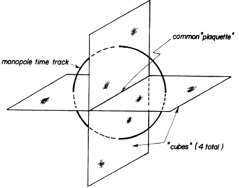
We claim that as $\gamma\rightarrow\infty$, the probability of having such a dominant configuration monopole decreases exponentially; accordingly there is only a thin population of minimal “strength monopoles” (and an even much thinner population of monopoles other than the “minimal strength” type). Hence it is presumably a very good approximation to describe the presence of monopoles as due solely to the dominant configuration of “minimal strength” monopoles.

In the case of the action (271), this means four 3-cube $\frac{2\pi}{4\pi}$-monopoles that encircle a common plaquette having a value corresponding to the nontrivial element of $\mbox{\bf{Z}}_{2}$. Consider by way of example the case where each of the four 3-cubes in this dominant configuration have the value $2\pi/5$ on five plaquettes (with the sixth “encircled” common plaquette having the value $\pm 2\pi$). Such a 3-cube configuration would, relative to a $\mbox{\bf{Z}}_{2}$ background flux (expected for large $\gamma$ and small $\beta$’s), behave as a $\frac{2\pi}{4\pi}$-monopole with a flux of $2\pi/5$ emanating from each of five plaquettes.

The dominant-configuration $\frac{2\pi}{4\pi}$-monopoles can be expected to occur with some low but nonzero density in the lattice near the phase border “2” even for large (but not too large) $\gamma$ values. Our suspicion, confirmed by calculations below, is that the degree of “first-orderness” of the phase transition at the boundary “2” is greater the smaller the chance that small deviations from $\mbox{\bf{Z}}_{2}$ (lying in $U(1)$) can, for the six plaquettes of a 3-cube, add up to a $\frac{2\pi}{4\pi}$-monopole (or, stated equivalently, add up to the length of the factor group $U(1)/\mbox{\bf{Z}}_{2}$).

As $\gamma$ decreases, an increasing number of $\frac{2\pi}{4\pi}$-monopoles is encountered. At the triple point (TP), where $\gamma\approx 1$, the presence of a larger number of $\frac{2\pi}{4\pi}$-monopoles than for very large $\gamma$ mitigates but does not eliminate the high degree of “first-orderness” characteristic of pure $\mbox{\bf{Z}}_{2}$ transitions (for which the deviations from $\mbox{\bf{Z}}_{2}$ (along $U(1)$) of six 3-cube plaquette variable values cannot sum to the length of the whole $U(1)/\mbox{\bf{Z}}_{2}$ due to $\gamma$ being too large).

In order to deal quantitatively with the effect of $\frac{2\pi}{4\pi}$-monopoles, and thereby with the question of how much of the behaviour of a pure $\mbox{\bf{Z}}_{2}$ transition is inherited by the phase transition at border “2” at the triple point, it is useful to define two new variables $U_{sign\;U(\Box)}(\Box)$ and $U_{BIO}(\Box)$:

$$U_{sign\;U(\Box)}(\Box)\stackrel{{\scriptstyle def}}{{=}}\left\{\begin{array}[]{l}+1\mbox{ if $U(\Box)$ closest to $e^{i0}\in\mbox{\bf{Z}}_{2}$}\\ -1\mbox{ if $U(\Box)$ closest to $e^{i\pi}\in\mbox{\bf{Z}}_{2}$}\end{array}\right.$$ (292)

The other new variable $U_{BIO}(\Box)$ (the subscript “$BIO$” is an acronym for Bianchi Identity Obeying) is defined as follows:

$$U_{BIO}(\Box)\stackrel{{\scriptstyle def}}{{=}}U_{sign\;U(\Box)}(\Box)\cdot$$ (293)

$$\cdot\left\{\begin{array}[]{l}+1\mbox{ \footnotesize for ordinary $\Box$ (i.e. {\em not} the encircled $\Box$ in the dominant config.)}\\ -1\mbox{ \footnotesize for $\Box$ encircled by four 3-cube $\frac{2\pi}{4\pi}$-monopoles in the dominant config.}\end{array}\right.$$

The variable $U_{BIO}(\Box)$ differs from the variable $U_{sign\;U(\Box)}(\Box)$ only by a sign change of $U_{sign\;U(\Box)}(\Box)$ in the case where the plaquette $\Box$ coincides with the “encircled” plaquette. The “encircled” plaquette is always present in the four 3-cube $\frac{2\pi}{4\pi}$-monopoles of the dominant monopole configuration.

Let us make the observation that the values assigned by the variable $U_{sign\;U(\Box)}(\Box)$ to the plaquettes of a 3-cube satisfy the $\mbox{\bf{Z}}_{2}$-Bianchi identity if the 3-cube is not a $\frac{2\pi}{4\pi}$-monopole; i.e., in our approximation, not one of the four 3-cube $\frac{2\pi}{4\pi}$-monopoles encircling a common plaquette in the dominant $\frac{2\pi}{4\pi}$-monopole configuration. Note, however, that the Bianchi identity is violated by the values assigned by the variable $U_{sign\;U(\Box)}(\Box)$ to the plaquettes of a 3-cube when there is a $\frac{2\pi}{4\pi}$-monopole. For instance, it is readily seen that for the very special $\frac{2\pi}{4\pi}$-monopole example given above ($U(\Box)=e^{i\frac{2\pi}{4\pi}\cdot 2\pi}=-1$ on the “encircled” plaquette; $U(\Box)=e^{i2\pi/5}$ on the remaining 5 plaquettes of the $\frac{2\pi}{4\pi}$-monopole 3-cube), the Bianchi identity is violated:

$$\prod_{\Box\in\partial(\frac{2\pi}{4\pi}-monopole\;3-cube)}U_{sign\;U(\Box)}(\Box)=(-1)\cdot 1^{5}=-1\neq 1$$ (294)

inasmuch as $U_{sign\;U(\Box)}(\Box)=-1$ for $U(\Box)=-1$ and $U_{sign\;U(\Box)}(\Box)=1$ for $U(\Box)=e^{i2\pi/5}$.

More generally, a $\frac{2\pi}{4\pi}$-monopole (which really just means a monopole modulo a $\mbox{\bf{Z}}_{2}$ background) consists of a configuration of plaquette variable values of a 3-cube that deviate continuously from elements of $\mbox{\bf{Z}}_{2}$ in such a way that the total sum of continuous deviations (lying in $U(1)$) from $\mbox{\bf{Z}}_{2}$ equals, modulo $4\pi$, $2\pi$ multiplied by the number of plaquettes for which the continuous deviations are centred at the nontrivial element of $\mbox{\bf{Z}}_{2}$. Note that in order to have a monopole, an odd number of the six plaquettes of a three cube must be near the nontrivial element (i.e., $2\pi$) of $\mbox{\bf{Z}}_{2}$

Even more generally, we have for a monopole modulo a $\mbox{\bf{Z}}_{N}$ background (i.e., a monopole for which the continuous $U(1)$ deviations from $Z_{N}\subset U(1)$ add up to a multiple of the length of the factor group $U(1)/\mbox{\bf{Z}}_{N}$):

$$\prod_{\mbox{\tiny$\Box\in$ 3-cube}}(U(\Box)g_{{}_{\tiny nearest}}(U(\Box))^{-1})=\prod_{\mbox{\tiny$\Box\in$ 3-cube}}g_{\tiny nearest}(U(\Box))\;\;\;\;\;\;\;(g_{\tiny nearest}(U(\Box))\in\mbox{\bf{Z}}_{N})$$ (295)

where $g_{\tiny nearest}(U(\Box))$ is defined as that element of $\mbox{\bf{Z}}_{N}$ which is nearest to $U(\Box)$:

$$dist^{2}(U(\Box),g_{\tiny\;nearest}(U(\Box)))\stackrel{{\scriptstyle def}}{{=}}inf\{dist^{2}(U(\Box),g^{\prime})\}\;\;\;\;(g^{\prime}\in\mbox{\bf{Z}}_{N})$$ (296)

where $dist^{2}(U(\Box),g^{\prime})$ denotes the squared distance from a plaquette variable value $U(\Box)$ and an element $g^{\prime}\in\mbox{\bf{Z}}_{N}$. We are really interested in $\mbox{\bf{Z}}_{6}=\mbox{\bf{Z}}_{2}\times\mbox{\bf{Z}}_{3}$ inasmuch as we are also interested in the modification of first-orderness due to an increasing number of monopoles modulo $\mbox{\bf{Z}}_{3}$ in going from large $\gamma$ to the triple point. However, for the purpose of exposition, we continue to use the example of monopoles modulo $\mbox{\bf{Z}}_{2}$.

With the modification of the variable $U_{sign\;U(\Box)}(\Box)$ that defines the variable $U_{BIO}(\Box)$, we have in $U_{BIO}(\Box)$ a variable that, for sufficiently large $\gamma$, assigns values to configurations of plaquettes that respects the $\mbox{\bf{Z}}_{2}$ Bianchi identities - also for $\frac{2\pi}{4\pi}$-monopole configurations (when the monopoles are of the dominant configuration type which is the only type for which the variable $U_{BIO}(\Box)$ is defined).

Note that the variable $U_{BIO}(\Box)$ differs from the variable $U_{sign\;U(\Box)}(\Box)$ only if there are $\frac{2\pi}{4\pi}$-monopoles. For $\gamma\rightarrow\infty$ such monopoles disappear and $U_{BIO}(\Box)=U_{sign\;U(\Box)}(\Box)\in\mbox{\bf{Z}}_{2}=\{+1,-1\}$. In going to smaller values of $\gamma$ in the phase with only $Z_{2}$ confining, an increasing range of fluctuations along $U(1)$ centred at the elements of $\{0,2\pi\}=\mbox{\bf{Z}}_{2}\subset U(1)$ provide alternative (Bianchi identity-obeying) configurations that supplement the essentially discrete group-valued plaquettes characteristic of large $\gamma$ configurations.

We want now to determine approximately the ($\gamma$ dependent) relation between the distributions of the two variables $U_{sign\;U(\Box)}(\Box)$ and $U_{BIO}(\Box)$. The average value of $U_{sign\;U(\Box)}(\Box)$ is estimated using the identity

$$\langle U_{sign\;U(\Box)}(\Box)\rangle=P(U_{BIO}(\Box)=+1)\langle U_{sign\;U(\Box)}(\Box)\rangle_{(U_{BIO}(\Box)=+1)}+$$ (297)

$$+P(U_{BIO}(\Box)=-1)\langle U_{sign\;U(\Box)}(\Box)\rangle_{(U_{BIO}(\Box)=-1)}$$

where $P(U_{BIO}(\Box)=+1)$ and $P(U_{BIO}(\Box)=-1)$ denote respectively the probabilities that $U_{BIO}(\Box)=+1$ and $U_{BIO}(\Box)=-1$ while $\langle U_{sign\;U(\Box)}(\Box)\rangle_{U_{BIO}(\Box)=+1}$ and $\langle U_{sign\;U(\Box)}(\Box)\rangle_{U_{BIO}(\Box)=-1}$ denote averages of $U_{sign\;U(\Box)}(\Box)$ subject respectively to the constraints that $U_{BIO}(\Box)=+1$ and $U_{BIO}(\Box)=-1$.

Denoting by $\xi=\xi(\gamma)$ the ($\gamma$ dependent) probability that a plaquette coincides with the “encircled plaquette” of the dominant $\frac{2\pi}{4\pi}$-monopole configuration, there obtains

$$\langle U_{sign\;U(\Box)}(\Box)\rangle_{U_{BIO}(\Box)=+1}=\frac{e^{\beta}\cdot 1+\xi e^{-\beta}\cdot(-1)}{e^{\beta}+\xi e^{-\beta}}$$ (298)

and

$$\langle U_{sign\;U(\Box)}(\Box)\rangle_{U_{BIO}(\Box)=-1}=\frac{e^{-\beta}\cdot(-1)+\xi e^{\beta}\cdot(+1)}{e^{-\beta}+\xi e^{\beta}}$$ (299)

Using

$$P(U_{BIO}(\Box)=+1)=\frac{1}{2}+\frac{1}{2}\langle U_{BIO}(\Box)\rangle$$ (300)

and

$$P(U_{BIO}(\Box)=-1)=\frac{1}{2}-\frac{1}{2}\langle U_{BIO}(\Box)\rangle$$ (301)

we have

$$\langle U_{sign\;U(\Box)}(\Box)\rangle=\frac{1}{2}\left(\frac{e^{\beta}-\xi e^{-\beta}}{e^{\beta}+\xi e^{-\beta}}+\frac{\xi e^{\beta}-e^{-\beta}}{\xi e^{\beta}+e^{-\beta}}\right)+\frac{1}{2}\left(\frac{e^{\beta}-\xi e^{-\beta}}{e^{\beta}+\xi e^{-\beta}}-\frac{\xi e^{\beta}-e^{-\beta}}{\xi e^{\beta}+e^{-\beta}}\right)\langle U_{BIO}(\Box)\rangle$$ (302)

$$\approx\langle U_{BIO}(\Box)\rangle(1-2\xi\cosh 2\beta)+2\xi\sinh 2\beta$$ (303)

where in the last step we have used that $\xi$ is assumed to be small.

We want now to calculate the jump in (284) in going from the phase with only $\mbox{\bf{Z}}_{2}$ confining to the totally Coulomb phase at the the triple point. That is, we want $\Delta\gamma_{eff}$ along the boundary “2” in Figure 22 as a function of $\gamma$:

$$\Delta\gamma_{eff}=\Delta(\gamma+\langle\sigma\rangle\frac{\beta_{crit}(\gamma)}{4})=\Delta\langle\sigma\rangle\frac{\beta_{crit}(\gamma)}{4}=\frac{\beta_{crit}(\gamma)}{4}\Delta\langle U_{sign\;U(\Box)}(\Box)\rangle.$$ (304)

where we have made the identification $\langle\sigma\rangle=\langle U_{sign\;U(\Box)}(\Box)\rangle$. Substituting (303) into (304) we get

$$\frac{\beta_{crit}(\gamma)}{4}\Delta\langle U_{sign\;U(\Box)}(\Box)\rangle=\frac{\beta_{crit}(\gamma)}{4}\Delta\langle U_{BIO}(\Box)\rangle(1-2\xi\cosh 2\beta(\gamma))$$ (305)

In our approximative procedure we identify $\Delta\langle U_{BIO}(\Box)\rangle$ with the jump in $\Delta\langle S_{\Box}\rangle$ for a $\mbox{\bf{Z}}_{2}$ gauge theory since the phase transition “2” at the triple point is determined from the phase of $\mbox{\bf{Z}}_{2}$.

Let us define a parameter $\beta_{BIO}$ as the action parameter $\beta$ in a $Z_{2}$ gauge theory which optimally reproduces the distribution of the variables $U_{BIO}(\Box)$ in the $U(1)$ theory (with the mixed action (271)) by using an action of the form

$$S=\beta_{BIO}\sum_{\Box}U_{BIO}(\Box).$$ (306)

In other words, $\beta_{BIO}$ is defined such that

$$\langle U_{BIO}(\Box)\rangle_{\mbox{\tiny in }U(1)\mbox{\tiny theory with }S=S(\beta,\gamma)}=\langle U_{BIO}(\Box)\rangle_{{\mbox{\scriptsize\bf{Z}}}_{2}\mbox{ \tiny theory with}S=\beta_{BIO}\sum_{\Box}U_{BIO}(\Box)}$$ (307)

We now want to obtain $\beta_{BIO}$ as a function of $\beta$ and $\xi$ (and hereby $\gamma$ inasmuch as $\xi=\xi(\gamma)$) by equating the ratio of the probabilities

$$\frac{P(U_{BIO}(\Box)=1)}{P(U_{BIO}(\Box)=-1)}$$ (308)

for the two actions $S=S(\beta,\gamma)$ and $S_{BIO}=\beta_{BIO}\sum_{\Box}U_{BIO}(\Box)$:

$$\frac{\overbrace{e^{\beta}}^{U_{sign\;U(\Box)}(\Box)=+1}+\overbrace{\xi e^{-\beta}}^{U_{sign\;U(\Box)}(\Box)=-1}}{\underbrace{e^{-\beta}}_{U_{sign\;U(\Box)}(\Box)=-1}+\underbrace{\xi e^{\beta}}_{U_{sign\;U(\Box)}(\Box)=+1}}=\frac{e^{\beta_{BIO}}}{e^{-\beta_{BIO}}}.$$ (309)

This procedure for estimating $\beta_{BIO}$ is somewhat errant in that Bianchi identities are ignored on both sides of equation (309) in various ways: first in the calculation of the ratio (308) and second, and presumably less importantly, in the simulation-by a-$\mbox{\bf{Z}}_{2}$ theory that defines $\beta_{BIO}$. The hope is that these error roughly cancel inasmuch as the same error is present on both sides of the equation.

Taking the logarithm of both sides of (309) and solving for $\beta_{BIO}$ yields

$$\beta_{BIO}=\beta+\frac{1}{2}\log\frac{1+\xi e^{-2\beta}}{1+\xi e^{2\beta}}$$ (310)

We want to use (310) to relate $\beta_{BIO}$ and $\beta_{crit}(\gamma)$ along the boundary “2” in Figure 22. Using that $\xi<<e^{\beta},\;1$ there obtains

$$\beta_{crit\;BIO}\approx\beta_{crit}(\gamma)+\frac{1}{2}\xi(e^{-2\beta}-e^{2\beta})=\beta_{crit}(\gamma)-\xi\sinh 2\beta.$$ (311)

Substituting (311) for $\beta_{crit}(\gamma)$ on the right-hand side of (305) yields

$$\Delta\gamma_{eff}=\frac{\beta_{crit}(\gamma)}{4}\Delta\langle U_{sign\;U(\Box)}(\Box)\rangle=\frac{1}{4}\beta_{crit\;BIO}\left(1+\frac{\xi\sinh 2\beta}{\beta_{BIO}}\right)\Delta\langle U_{BIO}(\Box)\rangle(1-2\xi\cosh 2\beta)=$$ (312)

$$=\frac{1}{4}\beta_{crit\;BIO}\Delta\langle U_{BIO}(\Box)\rangle\left(1+\xi\left(\frac{\sinh 2\beta}{\beta_{crit\;BIO}}-2\cosh 2\beta\right)\right).$$ (313)

Solving (311) for $\xi$ and substituting into (313) yields

$$\Delta\gamma_{eff}=\frac{1}{4}\beta_{crit\;BIO}\Delta\langle U_{BIO}(\Box)\rangle\left(1+(\beta_{crit}(\gamma)-\beta_{crit\;BIO})\left(\frac{1}{\beta_{crit\;BIO}}-\frac{2}{\tanh 2\beta}\right)\right).$$ (314)

From the literature [84] we have values for $\langle S_{\Box}\rangle_{{\mbox{\scriptsize\bf{Z}}}_{2}}=\Delta\langle U_{BIO}(\Box)\rangle$ and $\beta_{crit\;BIO}$. The quantity $\beta_{crit}(\gamma)-\beta_{crit\;BIO}$ is estimated graphically using a $U(1)$ phase diagram found in the literature[72] corresponding to the action (271). It is now finally possible to calculate $\Delta\gamma_{eff}$ at the triple point for the transition from the phase with only $\mbox{\bf{Z}}_{2}$ confining to the totally Coulomb-like phase.

It is indeed fortunate that the subtraction $\frac{1}{\beta_{BIO}}-\frac{2}{\tanh 2\beta}$ almost cancels thereby rendering our calculation of $\Delta\gamma_{eff}$ rather insensitive to the large uncertainty in the graphical estimate of $\beta_{crit}(\gamma)-\beta_{BIO}$. This means that the major contribution to the change in first-orderness in going from very large $\gamma$ to $\gamma\approx 1$ at the triple point is achieved simply by determining $\beta_{crit}(\gamma)$ by the condition that $\beta_{crit\;BIO}=\beta_{crit}(\gamma=\infty)$. This makes it possible to perform an analogous correction to the first-orderness in going from a pure $\mbox{\bf{Z}}_{3}$ theory to the triple point for an action $\gamma\cos\theta+\beta_{3}\cos\frac{\theta}{3}$ without having access to the phase diagram for the $U(1)$ theory with an action of this form (that we need for the graphical estimate of $\beta_{TP\;crit}(\gamma)-\beta_{{\mbox{\scriptsize\bf{Z}}}_{3}\;BIO}$).

In subsequent calculations, we shall make use of the fact that the probability $\xi$ of having a $\mbox{\bf{Z}}_{2}$ and a $\mbox{\bf{Z}}_{3}$ monopole must be roughly equal. The argument goes as follows: we can assume that essentially all monopoles present will be of the “minimal strength” type. In the case of the $SMG$, this means monopoles modulo a $\mbox{\bf{Z}}_{6}$ background: i.e., $\frac{2\pi}{12\pi}$-monopoles. These are built up of $U(1)$ elements close to $\mbox{\bf{Z}}_{6}$ such that the deviations from $\mbox{\bf{Z}}_{6}$ of six 3-cube plaquette variables add up to the full extent of $U(1)/\mbox{\bf{Z}}_{6}$. Of course it is still assumed that these “minimal strength” monopoles essentially only are found in dominant configuration of four 3-cubes that encircle a common plaquette But such a “minimal strength” monopole is a superposition of a $\mbox{\bf{Z}}_{2}$ and a $\mbox{\bf{Z}}_{3}$ monopole:

$$\frac{2\pi}{12\pi}=\frac{6\pi}{12\pi}-\frac{4\pi}{12\pi}$$ (315)

Assuming a rarity of $\pm\frac{2\pi}{4\pi}$-monopoles (i.e., $\pm\frac{6\pi}{12\pi}$-monopoles in the $12\pi$ normalisation) as well as $\frac{\pm 4\pi}{12\pi}$-monopoles (i.e., monopoles corresponding to the strength of a nontrivial element of the $\mbox{\bf{Z}}_{3}$ subgroup), monopoles are for all practical purposes exclusively of the $\frac{2\pi}{12\pi}$ type. And each of these “minimal strength” monopoles is formally a linear combination of exactly one $\mbox{\bf{Z}}_{2}$-monopole and one $\mbox{\bf{Z}}_{3}$-monopole. Hence these latter monopole types are “present” in essentially equal numbers.

As we would like to include not only the degree of first orderness inherited from $\mbox{\bf{Z}}_{2}$ at the triple point, but also that inherited from $\mbox{\bf{Z}}_{3}$, we need to generalise (304) and (313) which were derived for $\mbox{\bf{Z}}_{2}$ alone. The generalisation of (304) is obtained by varying (290):

$$\Delta\gamma_{eff}=\frac{\beta_{2}}{4}\Delta(\langle\sigma_{{\mbox{\scriptsize\bf{Z}}}_{2}}\rangle)+\frac{\beta_{3}}{9}\Delta(\langle\sigma_{{\mbox{\scriptsize\bf{Z}}}_{3}}\rangle)+\frac{\beta_{6}}{36}\Delta(\langle\sigma_{{\mbox{\scriptsize\bf{Z}}}_{6}}\rangle).$$ (316)

where the notation has been changed such that $\langle\sigma\rangle\stackrel{{\scriptstyle def}}{{=}}\langle U_{sign\;U(\Box)}(\Box)\rangle$ in (304) is in (316) denoted by $\langle\sigma_{{\mbox{\scriptsize\bf{Z}}}_{2}}\rangle$. For $\mbox{\bf{Z}}_{3}$ the analogous quantity is denoted by $\langle\sigma_{{\mbox{\scriptsize\bf{Z}}}_{3}}\rangle$ in (316). Moreover, we have the notational change $\beta_{crit\;BIO}\rightarrow\beta_{crit\;{\mbox{\scriptsize\bf{Z}}}_{2}}$ in going from (304) to (316). In (316) the analogous quantities for $\mbox{\bf{Z}}_{3}$ and $\mbox{\bf{Z}}_{6}$ are denoted respectively as $\beta_{crit\;{\mbox{\scriptsize\bf{Z}}}_{3}}$ and $\beta_{crit\;{\mbox{\scriptsize\bf{Z}}}_{6}}$. We have taken the $\beta_{6}$ term in (316) as being zero. This is presumably justified by the smallness of the $\mbox{\bf{Z}}_{6}$ “jump” contribution when treated (incorrectly) as being independent of $\mbox{\bf{Z}}_{2}$ and $\mbox{\bf{Z}}_{3}$.

In going to the new notation, (313) becomes (for $\mbox{\bf{Z}}_{2}$)

$$\Delta\gamma_{eff}=\frac{1}{4}\beta_{crit\;{\mbox{\scriptsize\bf{Z}}}_{2}}\Delta\langle S_{\Box}\rangle_{{\mbox{\scriptsize\bf{Z}}}_{2}}\left(1+\xi\left(\frac{\sinh 2\beta}{\beta_{crit\;{\mbox{\scriptsize\bf{Z}}}_{2}}}-2\cosh 2\beta\right)\right)$$ (317)

The generalisation that also includes the discontinuity inherited from $\mbox{\bf{Z}}_{3}$ that contributes to $\Delta\gamma_{eff}$ at the triple point transition from the phase with just the discrete subgroups $\mbox{\bf{Z}}_{2}$ and $\mbox{\bf{Z}}_{3}$ confining to the totally Coulomb-like phase is

$$\Delta\gamma_{eff}=\sum_{N\in\{2,3\}}\frac{1}{N^{2}}\beta_{crit\;{\mbox{\scriptsize\bf{Z}}}_{N}}\Delta\langle S_{\Box}\rangle_{{\mbox{\scriptsize\bf{Z}}}_{N}}\left(1+\xi\left(\frac{\sinh 2\beta}{\beta_{crit\;{\mbox{\scriptsize\bf{Z}}}_{N}}}-2\cosh 2\beta\right)\right).$$ (318)

From the argumentation above, we know that $\xi$ is expected to have the same value in both terms of (318).

In (318) it is seen that the subgroups $\mbox{\bf{Z}}_{2}$ and $\mbox{\bf{Z}}_{3}$ both contribute a term to $\Delta\gamma_{eff}$ at the triple point. Presumably it is a good approximation to calculate $\Delta\gamma_{eff}$ as if contributions from $\mbox{\bf{Z}}_{2}$ and $\mbox{\bf{Z}}_{3}$ are mutually independent inasmuch as these subgroups factorize at the multiple point. However, even in this approximation there will still be an indirect interaction between these subgroups via the continuum degrees of freedom in $U(1)$ and via the encircled plaquette in the dominant monopole configuration. Using (318), the contributions from $\mbox{\bf{Z}}_{2}$ and $\mbox{\bf{Z}}_{3}$ to $\Delta\gamma_{eff}$ are calculated and tabulated in Table 9.

Table 9: The quantity $\Delta\gamma_{eff}$ calculated using the appropriate terms in (318). In the last row, the quantities for $\mbox{\bf{Z}}_{6}$ are calculated (incorrectly) in a manner analogous to that used for $\mbox{\bf{Z}}_{2}$ and $\mbox{\bf{Z}}_{3}$. This procedure presumably overestimates the effect of $\mbox{\bf{Z}}_{6}$ contributions.

$$\begin{array}[]{|l|l|l|l|l|}\hline\cr&\beta_{crit\;{\mbox{\scriptsize\bf{Z}}}_{N}}&\Delta\langle S_{\Box}\rangle_{{\mbox{\scriptsize\bf{Z}}}_{N}}&\xi&\Delta\gamma_{eff}\\ \hline\cr\mbox{\bf{Z}}_{2}&0.44&0.44&0.04&0.047_{3}\\ \hline\cr\mbox{\bf{Z}}_{3}&0.67&0.56&0.04&0.039_{3}\\ \hline\cr(\mbox{\bf{Z}}_{6})&(1.00)&(0.13)&(0.0437)&(0.0033)\\ \hline\cr\end{array}$$ (319)

8.4 Calculating the enhancement factor for $1/\alpha_{U(1)}$ corresponding to the Planck scale breakdown of $U(1)^{3}$ to the diagonal subgroup

The two approximations that we have developed in order to gain an insight into the phase diagram for the group $U(1)^{3}$ - the independent monopole approximation and the group volume approximation - are more or less suitable according to whether the phase transitions are second or first order.

To determine the correct enhancement factor, we interpolate between the independent monopole approximation that gives this factor as 6 and the volume approximation that puts this factor at about 8. This interpolation is done by calculating the jump $\Delta W_{\Box\;``3"}$ in the Wilson operator at the boundary “3” transition at the TP (see Figure 22) that reflects the degree of first-orderness inherited at this transition from pure $\mbox{\bf{Z}}_{2}$ and $\mbox{\bf{Z}}_{3}$ transitions. As $\Delta\gamma_{eff}$ expresses the degree of first-orderness at the TP in going into the totally Coulomb-like phase, $\Delta W_{\Box\;``3"}$ is calculated using the assumption that it depends essentially on $\Delta\gamma_{eff}$.

The first approximation is the monopole condensate approximation in which the relevant quantity for which phase is realized is the amount of fluctuation in the convolution of the 6 plaquette variables enclosing a 3-cube.

In the second approximation - based on the group volume approximation - it turns out that to attain the multiple point in the hexagonal symmetry scheme, it is necessary to introduce additional parameters in the form of coefficients to 4$th$ and 6$th$ order perturbations to the Manton action. These additional parameters are used to get the free energy functions (corresponding to different phases) to coincide in parameter space at a point - “the” multiple point. This point is shared by what we expect is a maximum number of phases.

If, for example, the Coulomb to confining phase transition for a $Peter$-$U(1)$ subgroup is purely second order, this phase transition would not be expected to cause any change in at what value of the distance along another subgroup axis (e.g., the $Paul$-axis) the first identification-lattice point is encountered. The reason is that there is no discontinuous change in the degree of fluctuation in the $Peter$-plaquette variable in making the transition. In this case we expect the independent monopole approximation to work well.

On the other hand, if the phase transition is very strongly first order so that the fluctuations along the $Peter$-subgroup become discontinuously larger upon passing into the $Peter$ confinement phase, this can be expected to affect the threshold at which other subgroups go into confinement in a sort of “interaction effect”. In this situation the volume-approximation can be useful because it can take into account (and actually overestimates) the influence that fluctuations along different directions in the group can have on each other. The independent monopole approximation tends to ignore this effect.

Because the group volume approximation accounts for the interaction effect between fluctuations along different subgroups, it was necessary to use $4th$ and $6th$ order action terms in order to get a multiple point at which 12 phases convene (corresponding to continuous invariant subgroups; we neglect an infinity of discrete subgroups in this approximation). The effect of the higher order terms is the preferential enhancement of quantum fluctuations along the one dimensional (nearest neighbour) subgroup directions of the identification lattice thereby effectively eliminating the influence that fluctuations along one subgroup have on the fluctuations along another subgroup and vice versa.

In fact, the volume approximation effectively replaces the gauge group $G$ by its factor group $G/H$ when $H$ has confinement-like behaviour. This amounts to treating the fluctuations along the component of the group lying within the cosets $gH\;\;(g\in G)$ as being so large that, as far as Bianchi identities are concerned, we can regard the distribution of elements within the cosets of $H$ as essentially being that of the Haar measure .

8.4.1 The independent monopole condensate approximation - the calculation

In the independent monopole approximation, we can reach the multiple point using the Manton action alone (i.e., no higher order terms). The diagonal $U(1)$ subgroup to be identified with the $U(1)$ of the $SMG$ is that given by $\theta(1,1,1)$ in the coordinate choice (243).

The first identification lattice point met by this diagonal subgroup occurs for $\theta=2\pi$; i.e., the point $2\pi(1,1,1)$. Hence the quantisation rule $y/2\in{\bf Z}$ (for particles not carrying non-Abelian gauge coupling) is achieved by the naive continuum limit identification

$$\exp(i\theta(-))=\exp(iag_{1}A_{\mu}y/2)\;\;\;\mbox{for}\;\;\;y/2=1.$$ (320)

For $y/2=1$ (corresponding to $e^{+}_{L}$), the covariant derivative is

$$D_{\mu}=\partial_{\mu}-ig_{1}A_{\mu}.$$ (321)

The equation analogues to (236) for the diagonal subgroup (on the 3-dimensional identification lattice) is

$$\frac{\beta_{diag}}{2}(2\pi)^{2}=length(2\pi(1,1,1))=$$ (322)

$$=(2\pi)^{2}(1,1,1)\frac{\beta_{crit}}{2}\left(\begin{array}[]{ccc}1&\frac{1}{2}&\frac{1}{2}\\ \frac{1}{2}&1&\frac{1}{2}\\ \frac{1}{2}&\frac{1}{2}&1\end{array}\right)\left(\begin{array}[]{c}1\\ 1\\ 1\end{array}\right)=(2\pi)^{2}\frac{\beta_{crit}}{2}\cdot 6$$

for the multiple point. Contrary to the case of the non-Abelian couplings that are weakened by a factor $N_{gen}=3$ in going to the diagonal subgroup of $U(1)^{3}$, the $U(1)$ coupling at the multiple point is weakened by a factor 6 in going to the diagonal subgroup of $U(1)^{3}$. In general, the weakening factor in the hexagonal case in going from $U(1)^{N_{gen}}$ to the diagonal subgroup $U(1)$ along the direction $(1,1,\cdots,1)$ is $N_{gen}+\left(\begin{array}[]{c}N_{gen}\\ 2\end{array}\right)=N_{gen}(N_{gen}+1)/2$:

so that

$$g^{2}_{diag}=\frac{g^{2}_{crit}}{N_{gen}(N_{gen}+1)/2}.$$ (323)

8.4.2 The volume of groups scheme

In the earlier section 7.3.2, we have developed a means for calculating an effective inverse squared coupling having a directional dependence on $4th$ and $6th$ order action terms. We now calculate the effective inverse squared coupling (261) along the diagonal subgroup:

$$\frac{1}{e^{2}_{eff}(\vec{\xi})}\mbox{ (for $\xi=(1,1,1)$) }=$$ (324)

$$\left(B_{6}Y_{6\;\;comb}(diag)+\left(\frac{1}{e^{2}_{Manton}}+B_{4}Y_{4\;\;comb}(diag)\right)^{\frac{3}{2}}\right)^{\frac{1}{3}}=$$

$$=\left(\frac{-0.766}{e^{6}_{U(1)\;\;crit}}(-4\sqrt{\frac{3}{35}})+\left(\frac{2^{\frac{2}{3}}}{e^{4}_{U(1)\;\;crit}}+\frac{-0.146}{e^{4}_{U(1)\;\;crit}}\frac{2}{3}\sqrt{7}\right)^{\frac{3}{2}}\right)^{\frac{1}{3}}=$$

$$=1.34\cdot\frac{1}{e^{2}_{U(1)\;\;crit}}\;\;\;\mbox{ (in vol. approx.)}$$

From (322) we have that the inverse squared coupling corresponding to the diagonal subgroup of $U(1)^{3}$ is a factor 6 larger than $\frac{1}{e^{2}_{U(1)\;\;crit}}|_{\xi=(1,1,1)}\;$:

$$\frac{1}{e^{2}(diag)}=6\cdot\frac{1}{e^{2}_{eff}(\vec{\xi})}\left|{}_{\vec{\xi}=(1,1,1)}\right.=6\cdot 1.34=8.04$$ (325)

8.4.3 The calculation of the enhancement factor

We have seen that the enhancement factor $\frac{1/\alpha_{U(1)^{3}}}{1/\alpha_{U(1)}}$ has respectively the values 6.0 and $1.34\cdot 6.0$ according to whether the “independent monopole” or the “volume” approximation is used. These approximations tend respectively to ignore and to overestimate the dependence that fluctuations in one subgroup can have on which phase is realized along other subgroups or factor-groups. This interaction effect depends on the degree of first-orderness of the phase transition; this degree of first-orderness is used in our procedure to determine to what extent the pure “monopole approximation” should be “pushed” towards the “volume approximation”. We seek a combination of these two approximations - with the relative weight determined by the degree of first-orderness - that is to be embodied in the value of $\Delta\gamma_{eff}$ that subsequently is used in both steps of the calculation of the $U(1)$ continuum coupling. In this section, we use $\Delta\gamma_{eff}$ to determine the $U(1)$ coupling at the multiple point of a phase diagram for a $U(1)^{3}$ gauge group.

The correction for the degree of first-orderness will be implemented by choosing the “hop” $\Delta W=\Delta\langle\cos\theta\rangle$ in the Wilson operator at the TP transition to the totally Coulomb-like phase in such a way that it reflects the residual first-orderness. This transition obviously has to separate confinement-like and Coulomb-like phases for the continuum degrees of freedom. There are two possibilities - namely the TP transition at border “1” and the TP transition at border “3” corresponding let us say to respectively the jumps $\Delta W_{\Box\;TP\;``1"}$ and $\Delta W_{\Box\;TP\;``3"}$ in the Wilson operator.

But we now argue that $\Delta W_{\Box\;TP\;``1"}$ is not what we want because it doesn’t reflect the degree of “residual” first-orderness (at the TP) that is due to the $Z_{N}$ transition The reason has to do with $Z_{N}$ ($N=2,3$) being in the same phase on both sides of the border “1” at the TP. Accordingly, $\Delta W_{\Box\;TP\;``1"}$ cannot reflect the discrete group transition.

So it is the discontinuity $\Delta W_{\Box\;TP\;``3"}$ that we want to use to interpolate between the “independent monopole” and the “volume” approximation so as to obtain the enhancement factor $\frac{\alpha_{U(1)^{3}\;diag}}{\alpha_{U(1)\;crit}}$ that reflects the appropriate degree of first-orderness for the TP transition in going from confinement to Coulomb-like behaviour for the continuum degrees of freedom.

In order to estimate the residual “first-orderness” present at the multiple point in making the transition to the totally Coulomb-like phase from the phase(s) with confinement solely w.r.t to discrete subgroup(s), we shall use the already proposed scenario in which we speculate that the increased frequency of minimal strength monopoles (i.e., $\frac{2\pi}{4\pi}$ monopoles in the $4\pi$ normalisation implicit in (271)) is related to the fact that the phase transition along the border “2” in Figure 22 becomes less and less strongly first order as $\gamma$ decreases. That is, we speculate that the increasing role of minimal strength monopoles (in the $4\pi$ normalisation, the minimal strength $\frac{2\pi}{4\pi}$ monopoles are the only monopoles; in the $12\pi$ normalisation, there are, in addition to minimal and most abundant $\frac{2\pi}{12\pi}$ monopoles, also (less common) $\frac{6\pi}{12\pi}$- and $\frac{4\pi}{12\pi}$-monopoles) in typical plaquette configurations is the reason that the transitions to the totally Coulomb-like phase at border “2” and subsequently, also at border “3” in Figure 22 becomes less and less first order as $\gamma$ is diminished.

As mentioned just above, it is well known that, for $U(1)$, the phase transition at border “3” becomes second order at the tri-critical point (at a slightly negative value of $\gamma$) and continues as a second order phase transition for $\gamma$ values less than the tri-critical value $\gamma_{TCP}$. The above picture is not inconsistent with the results of numerical studies that clearly reveal even a pure $U(1)$ gauge theory with a Wilson action (i.e., a theory with $\gamma=0$) as having a weakly first order phase transition as evidenced by a “jump” $\Delta W_{\Box}$ in the Wilson operator $W_{\Box}$. Indeed one finds in the work of Jersàk[85] et al fits that relate the “jump” $\Delta W_{\Box}$ in the Wilson operator $W_{\Box}\stackrel{{\scriptstyle def}}{{=}}\langle\cos(\theta_{\Box})\rangle$ to $\Delta\gamma\stackrel{{\scriptstyle def}}{{=}}\gamma-\gamma_{TCP}$ where $\gamma_{TCP}$ denotes the value of $\gamma$ in the tri-critical point:

$$\Delta W_{\Box}=A(\gamma-\gamma_{TCP})^{\beta_{\mu}}$$ (326)

The values for $\gamma_{TCP}$ and $\beta_{\mu}$ are given respectively as $\gamma_{TCP}=-0.11\pm 0.05$ and $\beta_{\mu}=1.7\pm 0.2$ while the constant $A$ is deduced to be $A=0.68_{35}$. For $\gamma=0$ (corresponding to a Wilson action), there obtains $\Delta W_{\Box}=0.68(0.11)^{1.7}=0.016$.

Actually this latter discontinuity will be seen to be of interest to us because it can be shown that this jump is to a good approximation the jump $\Delta W_{\Box,\;``1"}$ encountered in crossing border “1” near the multiple point. The reasoning is as follows: the jump $\Delta W_{\Box,\;``1"}$ is to a good approximation constant along the phase border “1”; consequently, $\Delta W_{\Box,\;``1"}$ near the multiple point is essentially the same as that at $\gamma=1.01$ and $\beta=0$ which, in turn, is, by a simple change of notation, identical with the discontinuity $\Delta W_{\Box}$ at $\gamma=0$, $\beta=1.01$ that using (326) was found to have the value $\Delta W_{\Box}=0.016$.

So what is wanted for the purpose of calculating the enhancement factor is the jump $\Delta W_{\Box,\;``3"}$ encountered at the multiple point in traversing border “3” separating the totally Coulomb-like and totally confinement-like phases. What we have is a way to calculate $\Delta W_{\Box;\;``2"}$: this procedure relates $\Delta W_{\Box,\;``2"}$ to the cubic root[75, 86] of the quantity $\Delta\gamma_{eff}$ (see Section 8.3) encountered in crossing the border “2” at the multiple point. Were it not that the transition at border “1” is (weakly) first order but instead second order, then we would have had $\Delta W_{\Box,\;``1"}=0$ and

$$\Delta W_{\Box,\;``2"}=\Delta W_{\Box,\;``3"}=A(\Delta\gamma_{eff})^{\frac{1}{3}}\;\;\;\mbox{ (when $\Delta W_{\Box,\;``1"}=0$)}$$ (327)

where $A=0.252$. However, having argued that $\Delta W_{\Box,\;``1"}=0.16\neq 0$ corresponding to a weakly first order transition in crossing border “1” in the vicinity of the multiple point, we conclude on the grounds of continuity that this jump must be the difference in the “jumps” $\Delta W_{\Box,\;``2"}$ and $\Delta W_{\Box,\;``3"}$ in crossing respectively the borders “2” and “3” at the multiple point (see Figure 22). Recall that these jumps, observed in crossing the borders “2” and “3” near the multiple point are essentially assumed to be the residual effects of first-order pure discrete subgroup transitions at large $\gamma$. So in principle at least, the “jump” $\Delta W_{\Box;\;``3"}$ is obtained by correcting $\Delta W_{\Box\;``2"}$ (calculated by using (327)) by the amount of the “jump” $\Delta W_{\Box,\;``1"}$ in crossing border “1”. Using that $\Delta W_{\Box,\;``1"}$ is small, we make this correction in an approximate way by increasing $\Delta\gamma_{eff}$ in (327) by the corrective quantity

$$\Delta\gamma_{corr\;``1"}\stackrel{{\scriptstyle def}}{{=}}(\frac{\Delta W_{\Box,\;``1"}}{A})^{3}$$ (328)

obtained by inverting (327). In this approximation, we obtain

$$\Delta W_{\Box,\;``3"}\approx A(\Delta\gamma_{eff}+\Delta\gamma_{corr\;``1"})^{\frac{1}{3}}=$$ (329)

$$=A(\Delta\gamma_{eff}+(\frac{0.016}{0.252})^{3})^{\frac{1}{3}}$$

where we have used that $\Delta W_{\Box,\;``1"}=0.016$ in (328) which in turn has been used in (329). Strictly speaking, it is inconsistent to assume additivity in the “jumps” $\Delta W_{\Box,\;``1"}$, $\Delta W_{\Box,\;``2"}$, and $\Delta W_{\Box,\;``3"}$ (essential because of continuity requirements) and at the same time that both $\Delta W_{\Box,\;``2"}$ and $\Delta W_{\Box,\;``3"}$ are related to an appropriate $\gamma_{eff}$ by a cubic root law. Consistency requires $\Delta W_{\Box,\;``1"}=0$ corresponding to a second order transition. For small $\Delta W_{\Box,\;``1"}$, this inconsistency is not bothersome and the approximation (329) is good. In fact the corrective term $\Delta\gamma_{corr\;``1"}$ is so small so as not to yield a difference in $\Delta W_{\Box,\;``2"}$ and $\Delta W_{\Box,\;``3"}$ that is discernible to within the calculational accuracy.

Equation (329) provides a way of calculating the for us interesting $\Delta W_{\Box,\;``3"}$ at the multiple point. Various values of $\Delta W_{\Box,\;``3"}$ are tabulated in Table 10. These are calculated for different values of $\Delta\gamma_{eff}$ that in turn are obtained as combinations of the $\Delta\gamma_{eff}$ in Table 9 calculated for the $\mbox{\bf{Z}}_{2}$, $\mbox{\bf{Z}}_{3}$, and $\mbox{\bf{Z}}_{6}$ discrete subgroups of $U(1)$.

Before we use these various $\Delta W_{\Box,\;``3"}$ values to calculate the enhancement factor $\frac{\alpha_{U(1)^{3}\;diag}}{\alpha_{U(1)\;crit}}$, we need to develop a way of using the $\Delta W_{\Box,\;``3"}$ to interpolate between the “pure monopole” and the “volume” approximation. We now do this for the general case of any discontinuity $\Delta W_{\Box}$. In general, when there is a “jump” $\Delta W_{\Box}$, we estimate that we get the most correct enhancement factor $\frac{1/\alpha_{U(1)^{3}\;diag}}{1/\alpha_{U(1)}\;crit}$ by linearly interpolating between the enhancement factor “6” corresponding to the independent monopole approximation and the enhancement factor $1.34\cdot 6=8.04$ corresponding to the volume approximation. That is, the enhancement factor is calculated as

$$\left(\frac{1/\alpha_{U(1)^{3}\;diag}}{1/\alpha_{U(1)}}\right)_{actual}=\left(\frac{1/\alpha_{U(1)^{3}\;diag}}{1/\alpha_{U(1)}}\right)_{ind\;mono}+$$

$$+\frac{\eta}{\tau}\left[\left(\frac{1/\alpha_{U(1)^{3}\;diag}}{1/\alpha_{U(1)}}\right)_{vol}-\left(\frac{1/\alpha_{U(1)^{3}\;diag}}{1/\alpha_{U(1)}}\right)_{ind\;mono}\right]$$

$$=6+\frac{\eta}{\tau}[6(1.34-1)]$$ (330)

where $\frac{\eta}{\tau}$ is given by

$$\frac{\eta}{\tau}=\frac{\left(\frac{Coul\;fluc}{conf\;fluc}\right)^{2}_{ind\;\;mono}-\left(\frac{Coul\;fluc}{conf\;fluc}\right)^{2}_{actual}}{\left(\frac{Coul\;fluc}{conf\;fluc}\right)^{2}_{ind\;\;mono}-\left(\frac{Coul\;fluc}{conf\;fluc}\right)^{2}_{vol}}$$ (331)

and $\eta$ is defined as the numerator while $\tau$ the denominator on the right hand side of (331). Write

$$\left(\frac{Coul\;fluc}{conf\;fluc}\right)^{2}\stackrel{{\scriptstyle def}}{{=}}\frac{1-\langle\cos\theta\rangle_{Coul}}{1-\langle\cos\theta\rangle_{conf}}=1-\frac{\Delta W_{\Box}}{1-\langle\cos\theta\rangle_{conf}}$$ (332)

where in the last step we have used that $\langle\cos\theta\rangle_{Coul}=\langle\cos\theta\rangle_{conf}+\Delta W_{\Box}$.

Using that $\left(\frac{Coul\;fluc}{conf\;fluc}\right)^{2}_{ind\;mono}=1$ essentially by definition, we have using (331) and (332) that

$$\eta=\frac{\Delta W_{\Box}}{1-\langle\cos\theta\rangle_{conf}}=\Delta W_{\Box}/0.377$$ (333)

where in (333) we have used $\langle\cos\theta\rangle_{conf\;ph}=0.623$.

Various values of $\eta$ are tabulated in Table 10 corresponding to the values of $\Delta W_{\Box,\;``3^{\prime\prime}}$ that are also tabulated in the same Table.

The quantity $\frac{\eta}{\tau}$ are used to obtain the values for the enhancement factors $\frac{1/\alpha_{U(1)^{3}\;diag}}{1/\alpha_{U(1)}\;crit}$ tabulated in the final two columns of Table 10. The two columns correspond to $\frac{1/\alpha_{U(1)^{3}\;diag}}{1/\alpha_{U(1)}\;crit}$ for two different values of $\tau$. The first, corresponding to the roughest approximation, is for $\tau=1$ inasmuch as we make the approximation $\left(\frac{Coul\;fluc}{conf\;fluc}\right)^{2}_{vol}\approx 0$. The enhancement factors in the column at the extreme right hand side are obtained using a better estimate of $\tau$:

$$\tau=1-\left(\frac{Coul\;fluc}{conf\;fluc}\right)^{2}_{vol}=1-0.21=0.79.$$ (334)

The values of $\frac{1/\alpha_{U(1)^{3}\;diag}}{1/\alpha_{U(1)\;crit}}$ in the last column of Table 10 will appear in Table 11 in conjunction with the calculation of the Planck scale value of the continuum $U(1)$ fine-structure constant $1/\alpha_{U(1)\;Pl.\;scale}$.

Table 10: Enhancement factors given in the last four columns on the right are given for two ways of calculating $\tau$ as well as with and without $\Delta\gamma_{corr``1"}$ included in the calculation of $\Delta W_{\Box}$ in (329). For the quantity $\tau\stackrel{{\scriptstyle def}}{{=}}1-\left(\frac{Coul\;fluc}{conf\;fluc}\right)^{2}$ we have $\tau=1$ when confinement fluctuations are taken as infinite and $\tau=0.79$ when confinement fluctuations are taken as finite. The second and third columns contain $\Delta W_{\Box}$ calculated respectively with and without the quantity $\Delta\gamma_{corr``1"}$ in (329). The values for $\Delta\gamma_{eff}$ in the first column are taken from Table 9. The quantity $\eta$ in the fourth and fifth columns is defined in (331) and calculated according to (333) with and without the quantity $\Delta\gamma_{corr``1"}$ in the expression (329) for $\Delta W_{\Box}$.

Procedure $$\Delta\gamma_{eff} \Delta W_{\Box,``3"} \eta \frac{1/\alpha_{{U(1)}^{3}_{``diag"}}}{1/\alpha_{{U(1)}_{``crit"}}} \Delta\gamma_{corr``1"} \Delta\gamma_{corr``1"} \Delta\gamma_{corr``1"} \Delta\gamma_{corr``1"}=0 \Delta\gamma_{corr``1"} =0 \Delta\gamma_{corr``1"} =0 \tau=0.79 \tau=1 \tau=0.79 \tau=1 \langle\cos\theta\rangle_{Coul}=0.65 \langle\cos\theta\rangle_{Coul}=0.65 \frac{1}{2} \mbox{\bf{Z}}_{2} \mbox{\bf{Z}}_{2}+\mbox{\bf{Z}}_{3} \frac{0.047_{3}}{2}+ \frac{1}{2}(\mbox{\bf{Z}}_{2}+\mbox{\bf{Z}}_{3}) +\frac{0.039_{3}}{2} \frac{0.047_{3}}{2} \frac{1}{2}\mbox{\bf{Z}}_{2}+\mbox{\bf{Z}}_{3} +0.039_{3}$$ from (329) from (333) from (330) with with with Vol Approx: Haar (ideal) () 1 8.04 Haar, compact () 0.79 8.04 Mean field 7.29 7.02 Ideal ind mono 0 0 1 6 6 No discrete 0 0.016 0 0.042₄ 0 6.11₀ 6.08₇ 6 6 subgroups Using only: 0.047₃ 0.091₃ 0.091₁ 0.24₂ 0.24₂ 6.62₅ 6.49₄ 6.62₄ 6.49₃ Using 0.047₃+ : 0.039₃ 0.11₂ 0.11₁ 0.29₆ 0.29₆ 6.76₄ 6.60₄ 6.76₄ 6.60₃ Using : 0.088₇ 0.088₅ 0.23₅ 0.23₅ 6.60₇ 6.48₀ 6.60₆ 6.47₉ Using : 0.10₀ 0.10₀ 0.26₆ 0.26₆ 6.68₈ 6.54₃ 6.68₇ 6.54₂

8.5 Continuum critical coupling from critical $U(1)$ lattice coupling

The Planck scale prediction for the $U(1)$ fine-structure constant is to be obtained as the product of the enhancement factor and the continuum critical coupling that corresponds to the lattice critical coupling.

We have the enhancement factor in Table 10 (calculated using different approximations) but we have yet to translate the lattice $U(1)$ critical coupling into a continuum one. This is the purpose of this section.

We use a procedure analogous to that used by Jersàk et al[83]. In this work the continuum coupling is calculated numerically. Using Monte Carlo methods on the lattice, the Coulomb potential is computed and fitted to the formula proposed by Luck ([82]). In the Coulomb phase with the Wilson action, the fit yields

$$Wilson:\;\;\;\alpha(\beta)=0.20-0.24(\frac{\beta-\beta_{crit}}{\beta})^{0.39}\;=\;0.20-0.24(1-\frac{1.0106}{\beta})^{0.39}.$$ (335)

For the Villain action (in the Coulomb phase) the analogous result is

$$Villain:\;\;\;\alpha(\beta)=0.20-0.33(1-\frac{0.643}{\beta})^{0.52}.$$ (336)

It is of course our intention to substitute $\gamma_{eff}$ for what Jersak et al. designates as $\beta$. This is justified in as much as (335) is valid for $\beta\geq\beta_{crit}$; i.e., for $\beta$ lying within the Coulomb phase. The replacement of

$$\beta-\beta_{crit}$$ (337)

by

$$\gamma_{eff\;tot\;Coul\;ph}-\gamma_{eff.\;only\;{\mbox{\scriptsize\bf{Z}}}_{2}\;conf}\stackrel{{\scriptstyle def}}{{=}}\Delta\gamma_{eff}$$ (338)

is valid inasmuch as the phases separated by the phase boundary “2” in Figure 22 are both in the Coulomb phase as far as the continuum degrees of freedom are concerned. Values obtained for $\alpha$ using (335) with $\beta$ replaced by $\gamma_{eff}$ and $\beta-\beta_{crit}$ by $\Delta\gamma_{eff}$ are tabulated for various values of the latter in the third column of Table 11.

Table 11: Our Planck scale prediction for the $U(1)$ fine-structure constant is obtained as the product of the enhancement factor (from the last four columns of Table (10)) and the value of $1/\alpha_{cont}$ obtained from the critical value of the lattice parameter $\gamma_{eff}$ and the “jump” $\Delta\gamma_{eff}$ in this same quantity in crossing the phase border “3” (see Figure 22) at the multiple point. We list a number of combinations that differ according to how the discrete subgroups are treated w.r.t. whether the discrete subgroups are large enough to have the symmetry of the hexagonal identification lattice and how $\tau$ (see Table 10) is calculated as an indication of the sensitivity of our prediction to such details. The prediction marked with “$\bullet$” indicates the predicted value calculated in what we regard as the most correct manner. Also included are results for the Villian action where (336) has been used to calculate $\alpha(\beta)$. In this table, we use the same $\Delta\gamma_{eff}$ in both (335) and (336) (this is incorrect; see next table). In the Villian case, the $\Delta W_{\Box\;``3"}$ used in calculating the enhancement factor is calculated as $\Delta W_{\Box\;``3"}=0.16(\Delta\gamma_{eff})^{0.29}$ (this is the counterpart of (329) for the Wilson action) with $\Delta_{``1"\;corr}=0$). The coefficient “0.16” is estimated from Monte Carlo data in ([83]) and is rather uncertain.

$$\!\!\!\!\!\!\!\!\!\!\!\!\!\begin{array}[]{|l|l|l|l|l|l|l|l|}\hline\cr\vrule\lx@intercol\hfil\mbox{single $U(1)$}\hfil\lx@intercol\vrule\lx@intercol\\ \hline\cr\mbox{Procedure}&\Delta\gamma_{eff}&\alpha_{cont.}&1/\alpha_{cont.}&\lx@intercol\hfil\mbox{enh. fac Haar}\hfil\lx@intercol\vrule\lx@intercol&\lx@intercol\hfil\mbox{prediction $1/\alpha_{Pl.scale}$}\hfil\lx@intercol\vrule\lx@intercol\\ \cline{5-8}\cr&&&&\tau=0.79&\tau=1&\tau=.79&\tau=1\\ \hline\cr\mbox{Wilson action (using (\ref{contfor}))}&&&&&&&\\ \hline\cr\mbox{$\mbox{\bf{Z}}_{2}$ only with $\Delta\gamma_{corr``1"}$ in (\ref{jump3})}&0.047_{3}&0.128_{6}&7.77_{8}&6.62_{5}&6.49_{4}&51.5&50.5\\ \hline\cr\mbox{$\mbox{\bf{Z}}_{2}$ only without $\Delta\gamma_{corr``1"}$ in (\ref{jump3})}&0.047_{3}&0.128_{6}&7.77_{8}&6.62_{4}&6.49_{3}&51.5&50.5\\ \hline\cr\mbox{$\mbox{\bf{Z}}_{2}+\mbox{\bf{Z}}_{3}$ with $\Delta\gamma_{corr``1"}$ in (\ref{jump3})}&0.086_{6}&0.110_{8}&9.02_{1}&6.76_{4}&6.60_{4}&61.0&59.6\\ \hline\cr\mbox{$\mbox{\bf{Z}}_{2}+\mbox{\bf{Z}}_{3}$ without $\Delta\gamma_{corr``1"}$ in (\ref{jump3})}&0.086_{6}&0.110_{8}&9.02_{1}&6.76_{4}&6.60_{3}&61.0&59.6\\ \hline\cr\mbox{$\frac{1}{2}(\mbox{\bf{Z}}_{2}+\mbox{\bf{Z}}_{3})$ with $\Delta\gamma_{corr``1"}$ in (\ref{jump3} )}&0.043_{3}&0.130_{9}&7.64_{0}&6.60_{7}&6.48_{0}&50.5&49.5\\ \hline\cr\mbox{$\frac{1}{2}(\mbox{\bf{Z}}_{2}+\mbox{\bf{Z}}_{3})$ without $\Delta\gamma_{corr``1"}$ in (\ref{jump3})}&0.043_{3}&0.130_{9}&7.64_{0}&6.60_{6}&6.47_{9}&50.5&49.5\\ \hline\cr\mbox{$\frac{1}{2}\mbox{\bf{Z}}_{2}+\mbox{\bf{Z}}_{3}$ with $\Delta\gamma_{corr``1"}$ in (\ref{jump3})}&0.063_{0}&0.120_{6}&8.29_{2}&6.68_{9}&6.54_{3}&55.5\;\;\bullet&54.3\\ \hline\cr\mbox{$\frac{1}{2}\mbox{\bf{Z}}_{2}+\mbox{\bf{Z}}_{3}$ without $\Delta\gamma_{corr``1"}$ in (\ref{jump3})}&0.063_{0}&0.120_{6}&8.29_{2}&6.68_{7}&6.54_{2}&55.5\;\;\bullet&54.3\\ \hline\cr\hline\cr\mbox{Villian action (using (\ref{vil}))}&&&&&&&\\ \hline\cr\mbox{$\mbox{\bf{Z}}_{2}$ only}&0.047_{3}&0.11_{8}&8.46_{5}&6.45_{2}&6.35_{7}&54.6&53.8\\ \hline\cr\mbox{$\mbox{\bf{Z}}_{2}+\mbox{\bf{Z}}_{3}$}&0.086_{6}&0.091_{1}&10.9_{8}&6.53_{9}&6.42_{6}&71.8&70.6\\ \hline\cr\mbox{$\frac{1}{2}(\mbox{\bf{Z}}_{2}+\mbox{\bf{Z}}_{3})$}&0.043_{3}&0.12_{2}&8.22_{6}&6.44_{1}&6.34_{8}&53.0\;\;\bullet&52.2\\ \hline\cr\mbox{$\frac{1}{2}\mbox{\bf{Z}}_{2}+\mbox{\bf{Z}}_{3}$}&0.063_{0}&0.10_{6}&9.42_{4}&6.49_{1}&6.38_{8}&61.2\;\;\bullet&60.2\\ \hline\cr\end{array}$$ (339)

The $\gamma_{eff}$ used in Table 11 is that calculated in (284) to lowest order in $\hat{\theta}$. We want now to go to next order in $\hat{\theta}$. For the Wilson action suitable for having a phase confined solely w.r.t. $\mbox{\bf{Z}}_{2}$, the appropriate effective coupling is given by (283). We denote this improved effective coupling by $\gamma_{eff\;corr}$:

$$\gamma_{eff\;corr}=\gamma+\frac{\langle\sigma_{\mbox{\bf{Z}}_{2}}\rangle_{\hat{\theta}}\beta}{4}\langle\frac{\cos(\hat{\theta}/2)}{\cos\hat{\theta}}\rangle\approx\gamma+\frac{\langle\sigma_{\mbox{\bf{Z}}_{2}}\rangle_{\hat{\theta}}\beta}{4}\langle\cos^{-\frac{3}{4}}\hat{\theta}\rangle\mbox{ (Wilson action)}.$$ (340)

The improved $\gamma_{eff\;corr}$ for the Villian action case has the $\cos\hat{\theta}$ in the denominator in the average on the left-hand side of (340) removed corresponding to the Villian action being approximately a Manton action (having a second derivative that is $\hat{\theta}$-independent) instead of being equal to $\cos\hat{\theta}$ as in the Wilson case. So for the Villian action we have

$$\gamma_{eff\;corr}=\gamma+\frac{\beta}{4}\langle\sigma_{\mbox{\bf{Z}}_{2}}\rangle\cdot\langle\cos(\hat{\theta}/2)\rangle\approx\gamma+\frac{\beta}{4}\langle\sigma_{\mbox{\bf{Z}}_{2}}\rangle\cdot\langle\cos^{\frac{1}{4}}\hat{\theta}\rangle\;\;\;\mbox{(Villian action)}.$$ (341)

The effective couplings (340) and (341) are for respectively the Wilson and Villian actions. In both cases there can be a phase confined solely w.r.t. $\mbox{\bf{Z}}_{2}$. The analogous couplings for the Wilson and Villian actions in the case where there is a phase confined solely w.r.t. $\mbox{\bf{Z}}_{3}$ are given respectively by (342) and (343) below; i.e., by

$$\gamma_{eff\;corr}=\gamma+\frac{\beta}{9}\langle\sigma_{\mbox{\bf{Z}}_{3}}\rangle\langle\cos^{-\frac{8}{9}}\hat{\theta}\rangle\mbox{ (Wilson action)}$$ (342)

and

$$\gamma_{eff\;corr}=\gamma+\frac{\beta}{9}\langle\sigma_{\mbox{\bf{Z}}_{3}}\rangle\cdot\langle\cos^{\frac{1}{9}}\hat{\theta}\rangle\;\;\;\mbox{(Villian action)}.$$ (343)

Table 12 lists the $U(1)$ fine-structure constant at the Planck scale that is calculated for different combinations of contributions from $\mbox{\bf{Z}}_{2}$ and $\mbox{\bf{Z}}_{3}$ in the Wilson and Villian action cases using the improved effective couplings $\gamma_{eff\;corr}$ in (340), (341) (342) and (343).

Table 12: Here we use the improved effective couplings $\gamma_{eff\;corr}$ in (340) and (341) corresponding respectively to Wilson and Villian actions for which there is a phase confined solely w.r.t. $\mbox{\bf{Z}}_{2}$. The analogous improved effective couplings (342) and (343) are used respectively for the Wilson and Villian actions that can provoke phases confined solely w.r.t. $\mbox{\bf{Z}}_{3}$. Strictly speaking, for the improved calculation of $\Delta\gamma_{eff}$ - i.e., $\Delta\gamma_{eff\;corr}$ - we should (for say the Wilson action in the case where we have a phase confined solely w.r.t $\mbox{\bf{Z}}_{2}$) calculate as follows: $\Delta\gamma_{eff\;corr}=\frac{\beta}{4}\left(\langle\sigma\rangle_{Coul}\left\langle\frac{\cos\frac{\hat{\theta}}{2}}{\cos\hat{\theta}}\right\rangle_{Coul}-\langle\sigma\rangle_{conf}\left\langle\frac{\cos\frac{\hat{\theta}}{2}}{\cos\hat{\theta}}\right\rangle_{conf}\right)$ but because $\langle\sigma\rangle_{conf}<<\langle\sigma\rangle_{Coul}$ we have $\Delta\gamma_{eff\;corr}\approx\frac{\beta}{4}\left(\langle\sigma\rangle_{Coul}\left\langle\frac{\cos\frac{\hat{\theta}}{2}}{\cos\hat{\theta}}\right\rangle_{Coul}\right).$ We calculate $\Delta\gamma_{eff\;corr}$ iteratively inasmuch as the latter is needed to get $\Delta W$ which is needed to get $\langle\cos\hat{\theta}\rangle$ which in turn is needed to calculate $\Delta\gamma_{eff\;corr}$. The $\Delta W$ obtained iteratively using $\Delta\gamma_{eff\;corr}$ is also used in calculating the enhancement factor in Table 12. In the case of the Villian action, the cos$\hat{\theta}$ in the denominator of $\left\langle\frac{\cos\frac{\hat{\theta}}{2}}{\cos\hat{\theta}}\right\rangle$ is removed. The case having a phase confined solely w.r.t. $\mbox{\bf{Z}}_{3}$ is calculated in a way analogous to that for $\mbox{\bf{Z}}_{2}$ for respectively the Wilson and Villian action cases.

$$\!\!\!\!\!\!\!\!\!\!\!\!\!\!\!\!\!\begin{array}[]{|l|l|l|l|l|l|l|l|}\hline\cr\vrule\lx@intercol\hfil\mbox{corrected $U(1)$ }\hfil\lx@intercol\vrule\lx@intercol\\ \hline\cr\mbox{Procedure}&\Delta\gamma_{eff,\;corr}&\alpha_{cont.}&1/\alpha_{cont.}&\lx@intercol\hfil\mbox{enh. factor Haar}\hfil\lx@intercol\vrule\lx@intercol&\lx@intercol\hfil\mbox{prediction $1/\alpha_{Pl.scale}$}\hfil\lx@intercol\vrule\lx@intercol\\ \cline{5-8}\cr&&&&\tau=0.79&\tau=1&\tau=0.79&\tau=1\\ \hline\cr\mbox{Wilson action (using (\ref{contfor}))}&&&&&&&\\ \hline\cr\mbox{$\mbox{\bf{Z}}_{2}$ only with $\Delta\gamma_{corr``1"}$ in (\ref{jump3})}&0.060_{0}&0.122_{0}&8.19_{6}&6.67_{7}&6.53_{5}&54.7&53.6\\ \hline\cr\mbox{$\mbox{\bf{Z}}_{2}+\mbox{\bf{Z}}_{3}$ with $\Delta\gamma_{corr``1"}$ in (\ref{jump3})}&0.109_{4}&0.103_{1}&9.69_{7}&6.82_{6}&6.65_{3}&66.2&64.5\\ \hline\cr\mbox{$\frac{1}{2}(\mbox{\bf{Z}}_{2}+\mbox{\bf{Z}}_{3})$ with $\Delta\gamma_{corr``1"}$ in (\ref{jump3} )}&0.0561_{5}&0.123_{9}&8.07_{2}&6.66_{2}&6.52_{3}&53.8\;\;\bullet&52.7\\ \hline\cr\mbox{$\frac{1}{2}\mbox{\bf{Z}}_{2}+\mbox{\bf{Z}}_{3}$ with $\Delta\gamma_{corr``1"}$ in (\ref{jump3})}&0.0810_{8}&0.112_{9}&8.85_{4}&6.74_{8}&6.59_{1}&59.7\;\;\bullet&58.4\\ \hline\cr\hline\cr\mbox{Villian action (using (\ref{vil}))}&&&&&&&\\ \hline\cr\mbox{$\mbox{\bf{Z}}_{2}$ only}&0.0431_{8}&0.121_{7}&8.21_{9}&6.44_{1}&6.34_{8}&52.9&52.2\\ \hline\cr\mbox{$\mbox{\bf{Z}}_{2}+\mbox{\bf{Z}}_{3}$}&0.0811_{9}&0.0942_{4}&10.6_{1}&6.52_{9}&6.41_{8}&69.3&68.1\\ \hline\cr\mbox{$\frac{1}{2}(\mbox{\bf{Z}}_{2}+\mbox{\bf{Z}}_{3})$}&0.0404_{4}&0.124_{1}&8.05_{5}&6.43_{2}&6.34_{1}&51.8\;\;\bullet&51.1\\ \hline\cr\mbox{$\frac{1}{2}\mbox{\bf{Z}}_{2}+\mbox{\bf{Z}}_{3}$}&0.0594_{1}&0.108_{7}&9.20_{4}&6.48_{3}&6.38_{2}&59.7\;\;\bullet&58.7\\ \hline\cr\end{array}$$ (344)

9 Results of MPCP predictions compared with experimental values of fine-structure constants and conclusion

We use the principle of multiple point criticality to calculate the values of the three standard model gauge couplings. These agree with experiment to well within the calculational accuracy of 5 to 10%. In the context used here, the principle states that Nature seeks out the action parameter values in the phase diagram of a lattice gauge theory that correspond to the multiple point. At this point, a maximum number of phases convene. The gauge group is taken as the $N_{gen}$-fold Cartesian product of the standard model group: $SMG^{N_{gen}}$ where $N_{gen}=3$ is the number of fermion generations. So there is a $SMG$ factor for each family of quarks and leptons. This gauge group is referred to as the Anti Grand Unified Theory $(AGUT)$ gauge group. At the Planck scale, the gauge couplings are predicted to have the multiple point values corresponding to the diagonal subgroup of $SMG^{N_{gen}}$. The diagonal subgroup, which is isomorphic to the usual standard model group, arises as that surviving the Planck scale breakdown of the more fundamental $SMG^{N_{gen}}$ under automorphic symmetry operations.

In order to provoke the many phase that should convene at the multiple point - including those corresponding to confinement solely of discrete subgroups of the gauge group - we need a rather general action the parameters of which span a multi-dimensional phase-diagram space. In many cases, such phases would be called lattice artifacts because the boundary between such lattice-scale phases disappears in going to long wavelengths and what is distinguishable as a Coulomb-like phase at lattice scales becomes indistinguishable from a confining phase at large distances. Such phases are usually regarded as not being of physical significance because they depend on the presence of a lattice which has been introduced only as a calculational regulator that must leave no trace of its presence upon taking a continuum limit.

Our point of view is that a Planck scale lattice is one way of implementing the fundamental necessity of having a truly existing regulator at roughly the Planck scale. We would claim that field theories are intrinsicly inconsistent without the assumption of a fundamental regulator. While the lattice seems to play a fundamental role in our model, it is really only a way of manifesting the necessity of a fundamental regulator. We would of course hope that critical behaviour for any field theory formulated using other regulators (e.g., strings) would lead to approximately the same critical values for the coupling constants so that $MPC$ predictions based on the assumption that Nature had chosen a different regulator would not yield very different values for couplings than those obtained using a lattice regulator. Obtaining the same values of couplings when using different regulators would suggest that the principle of multiple point criticality has a validity that transcends the particulars of the regulator.

Our claim is then that even the presence of phases that are only distinguishable on a Planck scale lattice can have profound consequences for physics. And this is so despite the fact that such phases can - even though quantitatively distinguishable at the lattice scale (e.g., two phases with different finite correlation lengths) - become qualitatively indistinguishable at long distances. This situation is not unfamiliar in other situations. For example, at the triple point of water, three different phases can be accessed by suitable changes in intensive parameters by just a small amount. However, two of the three phases are not qualitatively distinct: at the tri-critical point, the distinction between liquid and vapour disappears. This however does not change the fact that all three phases are important in defining the triple point values of temperature and pressure.

Our Planck scale predictions for the gauge coupling constants come about as the product of the continuum value of the lattice critical coupling and the appropriate enhancement factor in going from the multiple point of $SMG^{3}$ to the diagonal subgroup.

The main difference between the Abelian and non-Abelian case is a factor two in the squared coupling weakening factor that comes from going from $SMG^{3}$ to the diagonal subgroup of $SMG^{3}$: the diagonal subgroup squared coupling for $U(1)$ is a factor

$$N_{gen}+\left(\begin{array}[]{c}N_{gen}\\ 2\end{array}\right)=(N_{gen}+1)N_{gen}/2=6$$ (345)

weaker than the critical values obtained from Monte Carlo data for a single $U(1)$. This is to be compared to the naively expected weakening factor $N_{gen}=3$ that is found for the non-Abelian couplings in going to the diagonal subgroup. The reason for the difference in the weakening factor in going to the diagonal subgroup of $SMG^{3}$ is that in the case of $U(1)$ there is the possibility of interaction terms $F_{\mu\nu\;Peter}F^{\mu\nu}_{Paul}$ in the Lagrangian (in the non-Abelian case, such terms are not gauge invariant). The indices $Peter,Paul,\cdots$ label the various $SMG$ factors of $SMG^{N_{gen}}$ (of which there are $N_{gen}=3$). Had the phase transition at the multiple point been purely second order, we would expect the enhancement factor for the inverse squared $U(1)$ coupling to be exactly $\frac{1}{2}N_{gen}(N_{gen}-1)=6.$ However, the fact that transitions between phases solely confined w.r.t. discrete subgroups and the totally Coulomb-like phase inherit a residual first-orderness from the pure discrete subgroup transitions leads to an enhancement factor larger than $\frac{1}{2}N_{gen}(N_{gen}-1)=6$. The enhancement factor for $U(1)$ is calculated using different approximations the result of which are tabulated in Table 10

The values we have calculated for the $U(1)$ gauge coupling (i.e., the values for the diagonal subgroup of $SMG^{3}$ at the multiple point of $SMG^{3}$) and the values calculated for the non-Abelian couplings are predicted to coincide with experimental values that have been extrapolated to the Planck scale using the assumption of a minimal standard model. In the renormalization group extrapolation procedure[25] used, we accordingly assume a desert with just a single Higgs ($N_{Higgs}=1$). The number of generations (families) is of course taken to be 3.

In doing the renormalization group extrapolation of experimental values to Planck scale, we start the running at the scale of $M_{Z}=91.176\pm 0.023$ using values from LEP experiments[24]. We also extrapolate the other way: we extrapolate our Planck scale predictions down to the scale of $M_{Z}$ so as these can be directly compared with experimental values of fine-structure constants. Predicted and experimental[25] values of the three fines-truce constants are compared at both the Planck scale and the scale of $M_{Z}$ are compared in Table 13. We have included predicted values obtained using several different variations in some details of our model. For the non-Abelian fine-structure constants, the naive continuum limit and the continuum-corrected continuum limit values are taken from our earlier work[3].

Table 13: Our predictions using slightly different calculational methods (approximations) and assumptions; these are compared with experimental values (Delphi results) extrapolated using the renormalization group to the Planck scale. The minimal Standard Model has been assumed in doing the extrapolation. The predicted values for $U(1)$ in the last eight rows are taken from Table 12 (with $\tau=0.79$).

SU(3)	$\alpha^{-1}(\mu_{Pl.})$	$\alpha^{-1}(M_{Z})$
Experimental values	53.6	9.25$\pm 0.43$
Continuum corrected continuum limit	$56.7\;\bullet$	12.${}_{8}\;\bullet$
Monopole correction	$56\pm 6\;\bullet$	$12._{1}\pm 6\;\bullet$
Naive continuum limit	$80._{1}$	$36._{2}$
SU(2)	$\alpha^{-1}(\mu_{Pl.})$	$\alpha^{-1}(M_{Z})$
Experimental values	49.2	30.10$\pm 0.23$
Continuum corrected continuum limit	$49.5\;\bullet$	29.${}_{8}\;\bullet$
Monopole correction	$48._{3}\pm 6\;\bullet$	$28._{5}\pm 6\;\bullet$
Naive continuum limit	$65._{1}$	$45._{3}$
U(1)	$\alpha^{-1}(\mu_{Pl.})$	$\alpha^{-1}(M_{Z})$
	($SU(5)$ norm. in parenthesis)	($SU(5)$ normalisation in parenthesis)
Experimental values:	54.8 (32.9)	98.70$\pm 0.21$ ($59.22\pm 0.13$)
Continuum corrected continuum limit	66 ($39._{6}$):	109.1 (65.5)
Naive continuum limit (w. enh. 6.8):	84.6(50.8)	127.7 (76.6)
Independent monopole approx.	30 (18)	73 (44)
$\mbox{\bf{Z}}_{2}$ (Wilson action):	54.7 (32.8)	97.8 (58.7)
$\mbox{\bf{Z}}_{2}$ (Villian action):	52.9 (31.7)	96.0 (57.6)
$\mbox{\bf{Z}}_{2}+\mbox{\bf{Z}}_{3}$ (Wilson action):	66.2 (39.7)	109.3 (65.6)
$\mbox{\bf{Z}}_{2}+\mbox{\bf{Z}}_{3}$ (Villian action):	69.3 (41.6)	112.4 (67.5)
$\frac{1}{2}(\mbox{\bf{Z}}_{2}+\mbox{\bf{Z}}_{3})$ (Wilson action):	53.8 (32.3)$\;\;\bullet$	96.9 (58.2)$\;\;\bullet$
$\frac{1}{2}(\mbox{\bf{Z}}_{2}+\mbox{\bf{Z}}_{3})$ (Villian action):	51.8 (31.1)$\;\;\bullet$	94.9 (57.0)$\;\;\bullet$
$\frac{1}{2}\mbox{\bf{Z}}_{2}+\mbox{\bf{Z}}_{3}$ (Wilson action):	59.7 (35.8)$\;\;\bullet$	102.8 (61.7)$\;\;\bullet$
$\frac{1}{2}\mbox{\bf{Z}}_{2}+\mbox{\bf{Z}}_{3}$ (Villian action):	59.7 (35.8)$\;\;\bullet$	102.8 (61.7)$\;\;\bullet$

In trying to estimate the uncertainty in our calculation of the $U(1)$ gauge coupling, two points of view can be taken:

a) we could take the viewpoint that we do not really know which of the phases characterised by being solely confined w.r.t. discrete subgroups should also convene at the multiple point in certain cases. In particular, we could claim that we do not know to what extent that $\mbox{\bf{Z}}_{2}-$ and $\mbox{\bf{Z}}_{3}$-like subgroups, in analogy to the U(1)-continuum, give rise to a hexagonal phase system at the multiple point. If this is the case, we have to let our lack of knowledge about such details of the phase diagram (and the multiple point chosen by Nature) be included in the uncertainty in our prediction.

b) we could take the standpoint that our choice of procedure for including the effects of having solely confining $\mbox{\bf{Z}}_{2}-$ and $\mbox{\bf{Z}}_{3}$-like subgroups at the multiple point is correct and that we accordingly can do our calculations based on a correct picture of the pattern of phases that convene at the multiple point, also w.r.t. solely confining discrete subgroups. In this case, uncertainties in our results are assumed to be due only to uncertainties in the Monte Carlo procedures used and in the approximations we use in our corrections of Monte Carlo data in order to get our predictions.

In the case a) we must regard the differences in predictions arising when $\mbox{\bf{Z}}_{2}-$ and $\mbox{\bf{Z}}_{3}$-like subgroups are taken into account in different ways as being a measure of the uncertainty. For the predicted $U(1)$ coupling at the Planck scale, this viewpoint leads to an estimated uncertainty of about 5%. We implement this point of view in Table 14 by averaging all combinations in which there is a $\frac{1}{2}\mbox{\bf{Z}}_{2}$ contribution. This results in an average of the combinations having $\mbox{\bf{Z}}_{3}$ and those having $\frac{1}{2}\mbox{\bf{Z}}_{3}$ as the contributions from $\mbox{\bf{Z}}_{3}$. This reflects our lack of certainty as to how the $\mbox{\bf{Z}}_{3}$ contribution should be treated.

In addition to this uncertainty, there will of course be the uncertainties in the Monte Carlo results which we have used which may be taken as 5%. Also, our corrections are presumably not performed to better than some 4%, so it is unlikely that the uncertainty in our prediction in case b) is less than 6.4%. In case a) we should rather take the uncertainty as being 8%. These percent-wise uncertainties concern the squared couplings referred to the Planck scale. These correspond to absolute Planck scale uncertainties of $4._{5}$ and $3._{5}$ in the inverse fine-structure constant in respectively the cases a) and b). But since the renormalization group correction consists basically of adding a rather well-determined constant to the inverse fine-structure constants, the absolute uncertainty in the $1/\alpha$’s is the same at all scales.

It is remarkable that in spite of these uncertainties being rather modest we have agreement with experiment within them!

It is interesting to formulate our predictions as a number that can be compared with the famous $\alpha^{-1}=137.036\dots$. From Table 14 we deduce that the phenomenologically observed value of $\alpha^{-1}$ decreases by $8.2\pm 0.5$ in going from low energies to that of $M_{Z}$:

$$137.036-(\alpha_{1}^{-1}(M_{Z})+\alpha_{2}^{-1}(M_{Z}))=137.036-(98.70\pm 0.23+30.10\pm 0.23)=8.2\pm 0.3$$ (346)

Our theoretical prediction for the famous $\alpha^{-1}=137.036$ is in the case a)

$$\alpha^{-1}_{1}(M_{Z})\;+\;\alpha^{-1}_{2}(M_{Z})\;+\;8.2\pm 0.5=$$ (347)

$$=99.4\pm 5\;+\;29.2\pm 6\pm 3.5\;+\;8.2\pm 0.3=136._{8}\pm 9$$

and in the case b)

$$\alpha^{-1}_{1}(M_{Z})\;+\;\alpha^{-1}_{2}(M_{Z})\;+\;8.2\pm 0.5=$$ (348)

$$=102.8\pm 3.5\;+\;29.2\pm 6\pm 3.5\;+\;8.2\pm 0.3=140._{2}\pm 8.$$

Table 14: The predicted values of $\alpha^{-1}(M_{Z})$ for $SU(3)$ and $SU(2)$, are obtained as the average of several calculational procedures. The first set of uncertainties comes from Monte Carlo data and from the approximation procedure that we used to get our predictions from the Monte Carlo critical couplings. The second set of uncertainties are the RMS deviations from the average value of $\alpha^{-1}(M_{Z})$ using the several different calculational procedures. The predicted $\alpha^{-1}(M_{Z})$ values for $U(1)$ and uncertainties arise as the result of the implementing the viewpoints a) and b) elaborated upon immediately above.

$$\begin{array}[]{|l|l|l|}\hline\cr&\alpha^{-1}(M_{Z})&\alpha^{-1}(M_{Z})\\ &predicted&experimental\\ \hline\cr SU(3)&12.4\pm 6\pm 6&9.25\pm 0.43\\ \hline\cr SU(2)&29.2\pm 6\pm 3.5&30.10\pm 0.23\\ \hline\cr U(1)&\begin{array}[]{cc}a)&99.4\pm 5\\ b)&102.8\pm 3._{5}\end{array}&98.70\pm 0.23\\ \hline\cr\end{array}$$ (349)

Since $\alpha_{s}^{-1}$ is rather small at experimental scales, the absolute uncertainty is percent-wise large at these scales. But really it is probably best to see our $\alpha_{s}$-prediction (at Planck scale) as a prediction of the logarithm of the ratio of the strong interaction scale to the Planck scale which then allows only a crude prediction of $\alpha_{s}(M_{Z})$. Note that the strong scale to Planck scale ratio is actually one of Dirac’s surprising $10^{20}$ factors! So this “large number” is found here as an exponential of an order one number that is proportional to the number of generations ($\pi^{2}$ in the denominator of the $\beta$-functions leads to couplings that walk slowly with scale).

Assuming the coexistence of more than one phase separated by transitions that are first order is roughly equivalent to assuming the principle of multiple point criticality. This principle offers the hope of a general explanation for the occurrence of fine-tuned intensive quantities in Nature. Indeed, the conspicuous values taken by a number of physical constants - e.g., the vanishing effective cosmological constant, the fine-structure constants, $\Theta_{QCD}$ - have values that coincide with values obtained if it is assumed that Nature seeks out multiple point values for intensive parameters.

As mentioned above, multiple point values of intensive parameters occur in the presence of coexisting phases separated by first order transitions. Such coexistence could be enforced by having fixed but not fine-tuned amounts of extensive quantities. We have shown in recent work[5, 6] that the enforced coexistence of extensive quantities in spacetime is tantamount to having long range nonlocal interactions of a special type: namely interactions that are identical between fields at all spacetime points regardless of the spacetime distance between them. Such omnipresent nonlocal interactions, which can be described by a very general form of a reparameterization invariant action, would not be perceived as non-locality but rather most likely absorbed into physical constants. Even still, the presence of nonlocal interactions opens the possibility for having contradictions of a type reminiscent of the “grandfather paradox” naively encountered in “time machines”. However, we can show[2] that generically there is a “compromise” that averts paradoxes. It is interesting that this solution coincides with multiple point values of intensive quantities such as fine-structure constants and the cosmological constant. Hence one can speculate that it is a mild form of non-locality, intrinsic to fundamental physics, that is the underlying explanation of Nature’s affinity for the multiple point.

In a sense, the MPCP can also be said to have some predictive power as to the form assumed by the “the true action of Nature”. For example, if two proposed actions differ in the number of “phases” that can be brought together at a multiple point, the action that can bring together the larger number of phases would, according to the MPCP, come closer to being the “true action of Nature”. The same sort of argument may be applicable to proposed candidates for gauge groups: having a MPCP would favour a non-simple gauge group over a simple gauge group. While the implementation of the MPCP can be be said to be rather complicated technically, the underlying idea is extremely eloquent in its simplicity. This combined with the noteworthy accuracy with which a number of constants of Nature are predicted makes the MPCP a serious contender as an important link in our understanding of fundamental physics.

9.1 Loose speculations as to the relevance of the MPCP in the evolution of living organisms

In concluding this thesis, it is interesting to speculate as to the possibe wider range of applicability of the principle of multiple point criticality. In 1992, while I held an associate professorship at the Royal Danish School of Pharmacy, I put forth the idea[87, 88] that complicated biological regulatory mechanisms may achieve maximum stability by seeking out the multiple point in the parameter space of what is probably the intractably complicated action of a biological system. By seeking out the multiple point, Nature can utilize easy access to the maximum number of phases as a means of maximizing the stability of the complicated forms of regulation required for the dynamical stability of a biological system in the presence of an ever-changing enviornment. Being at the multiple point is tantamount to being simultaneously on the verge of undergoing a phase transition to any one of many more or less ordered phases. A system in the most ordered phase (a “Coulomb-like” phase characterised by degrees of freedom all of which are correllated over long distances) that at the same time is infinitesimally close to the multiple point has access to plethora of phases that are more or less chaotic (depending on the degree of “first-orderness” of the transition) w.r.t. any of the various degrees of freedom (analogous for example to $U(1)$ degrees of freedom, $SU(3)/\mbox{\bf{Z}}_{3}$ degrees of freedom, $\mbox{\bf{Z}}_{2}$ degrees of freedom, etc., etc. in the lattice gauge theory implementation of the MPCP with the gauge group $SMG^{3}$) simply by effecting infinitesimal changes in intensive parameters. In being at the multiple point, a system is at what can be said to be the ultimative “edge of chaos”.

The idea that the multiple point criticality principle might apply in some sense to biological systems occurred to me in connection with work I have been doing together with John Ipsen (The Technical University of Denmark) and Holger Bech Nielsen (The Niels Bohr Institute). First we were interested in the use of a lattice gauge theory formulation as a way of implementing the constraint of self-avoiding surfaces in computer simulations of lipid membranes. Most recently we have been involved in designing ways of doing computer simulations using Kalb-Ramond lattice gauge theories as a way of introducing a “volume fugacity”. Together with the usual area and topological fugacities as control parameters, having this additional parameter will allow simulation of membrane models that are considerably more complicated that those presently tractable. This ongoing work on membranes springs from earlier work with Ole Mouritsen and also Peter Leth Christiansen (both from The Technical University of Denmark) the focus of which was a Cand. pharm. Ph.D. student who wanted to do serious studies of the way in which pharmaceutical agents affect the very complicated interdependence of the internal state of a lipid membrane and the activity of membrane-bound proteins. Phase transitional regions turn out to play an extremely important role in the mechanism by which pharmaceutical agents exert physiologically observable effects as we showed in a series[89, 90, 91, 92, 93] of work. It is really this work that suggested the validity of the principle of multiple point criticality for biological systems inasmuch as it is well-known that biological membranes are rather meticulously maintained at values of intensive parameters (i.e. temperature) that lie very close to a phase transition.

It is interesting that my suggestion that life processes seek out the stability and regulatory flexibility afforded by being at the multiple point is an idea that, superficially at least, bears a strong resemblence to a school of thought that has emerged at the Santa Fe Institute in recent years. The first essential element in this thinking, which to a large extent has been put forth by Stuart Kauffman and Christopher Langton (both at the Santa Fe Institute), is that order, and in particular self-replicability, tend inherently to emerge in systems having sufficient complexity. Kauffman’s view is that the dynamics of any sufficiently complicated system of agents (e.g., cells, genes, protein fragments, business corporations, members of a democracy, etc.) that registers input and generates output that subsequently is interpreted as input by other perhaps neighbouring agents will evolve basins of attraction that entrap the system into persistent patterns possessing a high degree of diffrentiation that interact in a highly organized, stable and self-sustaining way. This is sometimes referred to as “catalytic closure”. In Kauffman’s words, one has the unavoidable emergence of “order for free”.

Kauffman and Langton go even further: having made the case for “order for free”, they inquire as to the conditions under which the evolution of self-organized systems is maximally robust when faced with the perpetual changes in the enviornment that must be accommodated by a self-organized system if it is to survive. In considering this problem, Kauffman is lead to propose that the control of self-organized order also emerges spontaneously. How does a systems evolves a system of contol that assures maximum adaptability? Here adaptability refers to the ability of a system to adjust the system of “links” between its agents so that the system fits its enviornment over time. Obviously a system with a deficiency of such links will not be well-suited to a cooperative effort on the part of its agents in devising an optimal survival strategy in the face of external changes. The uncoordinated performance of non-percollating structures cannot contribute optimally to the solution of a problem (e.g., a change in the enviornment) faced by the system as a whole. What is perhaps more surprising is that an over-abundance of links between agents is also debilitating for a system challenged by changes in the enviornment. Such systems are frozen into inactivity by the constraints of too many links and hence are unable to be optimally innovative in solving problems. It seems that self-organized systems need, for optimal adaptability, to have a mechanism for dynamically “self-tuning” the system of links between its agents in such a way as to be able to deal optimally with coevolutionary external changes.

Langton may have found a clue as to how such such a dynamical fine-tuning mechanism comes about. Using systems of cellular automata as a simplified form of a parallel-processing (Boolean) network, Langton finds static and propagating structures at the phase transition separating chaotic and ordered regimes that can support information storage and tranmission as well as phenomena that can be interpreted as a form of information processing. Kauffman and Langton propose that at levels in systems which must coordinate complicated tasks, selection attains a near-universal “poised” state that hovers at the phase transition between spontaneous order and chaos. In the words of C. Langton and N. Packard, it may be that life seeks out and is sustained at the edge of chaos.

The principle of multiple point criticality, in asserting that the universe cannot avoid seeking out multiple point values of intensive parameters, is essentially asserting that the fundamental laws of physics reside at the “edge of chaos”.

The point I wish to make is that the multiple point (i.e., “the ultimative edge of chaos”) functions as an attractor that can provide a useful stabilisation mechanism that quite plausibly could be inherited by biological systems as the tendency of evolving life processes to be maintained at the edge of chaos. This would be consistent with the idea of Kauffman and Langton that selection results in a chain of biological systems in the course of evolution that perpetually seek out and “ride along” on the ever-changing “edge of chaos” as the way of achieving the most sustainable evolution of ever more complicated organisms. Recent discussions[94] and the exchange of notes[95] with Stuart Kauffman in Santa Fe reveal that he fully shares my sentiments as to the importance of exploring the idea that the apparent tendency of biological systems to cling to the edge of chaos in the course of evolution may be a manifestation of a fundamental physical principle of multiple point criticality. We have made plans for continuing this avenue of investigation in the months to come.

10 Acknowledgements

My heart-felt thanks and admiration go to Holger Bech Nielsen - great friend, inspiring teacher and enthusiastic colleague without whom the writing of a Ph.D. thesis (and physics) undoubtedly wouldn’t have been nearly so much fun (and any thesis would have turned out much differently!). To Erling Jensen I am grateful for having learned the pleasures of not always taking established thinking too seriously. To Søren Ventegodt go my deep-felt thanks because his (untamed) enthusiasm is huge enough also to bring me in out of the cold. I am also very grateful for useful and inspiring interactions in various periods with Dino Butorovic, Ivica Picek, Niels Brene, Leah Mizrachi, Kent Jørgensen, Ole Mouritsen, John Ipsen, Igor Volovich, Christian Surlykke, Sven Erik Rugh, Larisa Laperashvili, Collin Froggatt and Kasper Olsen. My thanks also go to many other kind and supportive people at The Niels Bohr Institute.

30 May 96 alf

11 Appendices

11.1 Appendix: Haar measure to next to leading order

For the contribution to $``-\beta F"$ from the confining degrees of freedom, the most important next order correction to the tangent space or weak coupling approximation comes from taking into account the influence on the Haar measure arising from the curvature of the group manifold for a non-Abelian Lie group $G$. In the neighbourhood of the unit element the exponential map $\;\;\;exp:\mbox{Lie algebra}\rightarrow\mbox{Lie group}\;\;\;\;\;$ is one to one, and it may be used to induce in the Lie algebra a measure from the Lie group. However, for a group manifold with curvature, it is only infinitesimally close to the unit element that the correct Haar measure coincides with the “flat” measure:

$$d^{{\cal H}aar}U=d^{{\cal H}aar}(exp(A))=\rho_{flat}\;\;d^{d}A/\sqrt{2}=\frac{d^{d}A/\sqrt{2}}{vol(G)}.$$ (350)

Here, as in the preceding text, the uniform Haar measure density $\rho_{flat}$ is taken as $\rho_{flat}=\frac{1}{vol(G)}.$

Because a left translation in the Lie algebra and in the Lie group do not coincide exactly for a non-Abelian group (due to curvature), the Haar measure that is to be invariant under left translation on the group will deviate from being constant relative to that on the algebra. Consider all the group elements corresponding to the Lie algebra elements in a small volume element at the origin of the Lie algebra. These group elements correspond, after left (or right) translation by say the group element $exp(\mbox{\bf{A}})$, to a volume at the translated position in the Lie algebra that is expanded by some factor relative to the small volume at the origin. Invariance of the Haar measure on the group manifold under left (or right) group multiplication by $exp(\mbox{\bf{A}})$ requires therefore a compensating factor in the Haar measure density $\rho^{{\cal H}aar}(\mbox{\bf{A}})$ at the left translated position $exp(\mbox{\bf{A}})$ on the group manifold relative to the density at the unit element of the group.

Let $\mbox{\bf{B}}^{1},\mbox{\bf{B}}^{2},\cdots\mbox{\bf{B}}^{j=dim(G)}$ be infinitesimal displacements in the $dim(G)$ independent directions of the Lie algebra at the origin of the Lie algebra.

Designate by $L_{exp({\mbox{\scriptsize\bf{A}}})}$ the operation of left multiplication in the group: $L_{exp({\mbox{\scriptsize\bf{A}}})}g=\exp(\mbox{\bf{A}})g\;\;(\exp(\mbox{\bf{A}}),\;g\in G)$.

Denote by $\mbox{{\bf{\sf T}}}_{L(A)}\mbox{\bf{B}}^{j}$ the Lie algebra vector that is vectorially added to the Lie algebra vector A when the group element $exp(\mbox{\bf{B}}^{j})$ is translated by $L_{exp({\mbox{\scriptsize\bf{A}}})}$; i.e., $L_{exp({\mbox{\scriptsize\bf{A}}})}exp(\mbox{\bf{B}}^{j})=exp(\mbox{\bf{A}}+\mbox{{\bf{\sf T}}}_{L(A)}\mbox{\bf{B}}^{j})$.

In the “flat” or tangent space approximation we have $\mbox{\bf{A}}+\mbox{{\bf{\sf T}}}_{L(A)}\mbox{\bf{B}}^{j}=\mbox{\bf{A}}+\mbox{\bf{B}}^{j}$ corresponding to the Lie algebra composition rule of simple vector addition when the group operation $L_{exp({\mbox{\scriptsize\bf{A}}})}exp(\mbox{\bf{B}}^{j})$ is referred to the Lie algebra.

For a group manifold with curvature, the Lie algebra composition rule - we denote it with the symbol “$+^{\prime}$” - is more complicated. Under the action of $L_{exp(\mbox{\bf{A}})}$ on the group we have $\mbox{\bf{A}}+\mbox{{\bf{\sf T}}}_{L(A)}\mbox{\bf{B}}^{j}=\mbox{\bf{A}}+^{\prime}\mbox{\bf{B}}^{j}$.

Denote by $\Delta V$ the volume element spanned by the $\mbox{\bf{B}}^{j}$’s at the origin of the Lie algebra: $\Delta V=\mbox{\bf{B}}^{1}\wedge\mbox{\bf{B}}^{2}\wedge\cdots\wedge\mbox{\bf{B}}^{dim(G)}$. Let C be an infinitesimal vector specifying a point within the volume $\Delta V$.

For one of the infinitesimal displacements $\mbox{\bf{B}}^{j}$ at the origin of the Lie algebra, the effect of the group operation $L_{exp({\mbox{\scriptsize\bf{A}}})}$ referred to the Lie algebra can be expressed as

$$(\mbox{\bf{A}}+\mbox{{\bf{\sf T}}}_{L(A)}\mbox{\bf{B}})^{j}=(\mbox{\bf{A}}+^{\prime}\mbox{\bf{B}})^{j}=(\mbox{\bf{A}}+^{\prime}\mbox{\bf{0}})^{j}+(d(\mbox{\bf{A}}+^{\prime}\;\cdot)_{{}_{\mbox{\scriptsize\bf{0}}}})^{j}_{k}\mbox{\bf{B}}^{k}=\mbox{\bf{A}}^{j}+d((\mbox{\bf{A}}+^{\prime}\;\cdot)_{{}_{\mbox{\scriptsize\bf{0}}}})^{j}_{k}\mbox{\bf{B}}^{k}$$ (351)

where

$$d((\mbox{\bf{A}}+^{\prime}\cdot)_{{}_{\mbox{\scriptsize\bf{0}}}})^{j}_{k}=\frac{\partial(\mbox{\bf{A}}+^{\prime}\mbox{\bf{C}})^{j}}{\partial\mbox{\bf{C}}^{k}}\mid_{{}_{\mbox{\scriptsize\bf{C}}}=_{\mbox{\scriptsize\bf{0}}}}.$$ (352)

It follows that the $\mbox{\bf{B}}^{j}$ at the origin of the Lie algebra has become

$$(\mbox{{\bf{\sf T}}}_{L(A)}\mbox{\bf{B}})^{j}=\sum_{k}\frac{\partial(\mbox{\bf{A}}+^{\prime}\mbox{\bf{C}})^{j}}{\partial\mbox{\bf{C}}^{k}}\mid_{{}_{\mbox{\scriptsize\bf{C}}}=_{\mbox{\scriptsize\bf{0}}}}\mbox{\bf{B}}^{k}$$ (353)

under the group operation $L_{exp({\mbox{\scriptsize\bf{A}}})}$.

The volume element $\Delta V=\mbox{\bf{B}}^{1}\wedge\mbox{\bf{B}}^{2}\wedge\cdots\wedge\mbox{\bf{B}}^{dim(G)}$ at the origin of the Lie algebra expands into the volume $\mbox{{\bf{\sf T}}}_{L(A)}\Delta V$ under the group operation $L_{exp({\mbox{\scriptsize\bf{A}}})}$. We can write

$$\mbox{{\bf{\sf T}}}_{L(A)}\Delta V=\mbox{{\bf{\sf T}}}_{L(A)}\mbox{\bf{B}}^{1}\wedge\mbox{{\bf{\sf T}}}_{L(A)}\mbox{\bf{B}}^{2}\wedge\cdots\wedge\mbox{{\bf{\sf T}}}_{L(A)}\mbox{\bf{B}}^{dim(G)}$$ (354)

$$=\frac{\partial(\mbox{\bf{A}}+^{\prime}\mbox{\bf{C}})^{1}}{\partial\mbox{\bf{C}}^{k}}\mid_{{}_{\mbox{\scriptsize\bf{C}}}=_{\mbox{\scriptsize\bf{0}}}}\mbox{\bf{B}}^{k}\wedge\cdots\wedge\frac{\partial(\mbox{\bf{A}}+^{\prime}\mbox{\bf{C}})^{dim(G)}}{\partial\mbox{\bf{C}}^{m}}\mid_{{}_{\mbox{\scriptsize\bf{C}}}=_{\mbox{\scriptsize\bf{0}}}}\mbox{\bf{B}}^{m}$$

$$=\left\|\frac{\partial(\mbox{\bf{A}}+^{\prime}\mbox{\bf{C}})^{j}}{\partial\mbox{\bf{C}}^{k}}\left|{}_{{}_{\mbox{\scriptsize\bf{C}}}=_{\mbox{\scriptsize\bf{0}}}}\right.\right\|(\mbox{\bf{B}}^{1}\wedge\mbox{\bf{B}}^{2}\wedge\cdots\wedge\mbox{\bf{B}}^{dim(G)})=det(d(\mbox{\bf{A}}+^{\prime}\cdot)_{{}_{\mbox{\scriptsize\bf{0}}}})\Delta V$$

Really, the map $(\mbox{\bf{A}}+^{\prime}\cdot)_{{}_{\mbox{\scriptsize\bf{0}}}}$ is the composed map consisting of

1. a map from very near the origin of the Lie algebra to very near the identity of the group;

2. left translation to very near the element $exp(\mbox{\bf{A}})$ in the group and

3. a log mapping back to the Lie algebra from very near the group element $exp(\mbox{\bf{A}})$.

Linearising this composed map we get

$$d(\mbox{\bf{A}}+^{\prime}\cdot)_{{}_{\mbox{\scriptsize\bf{0}}}}=d(exp^{-1}\circ L_{exp({\mbox{\scriptsize\bf{A}}})}\circ exp)_{{}_{\mbox{\scriptsize\bf{0}}}}$$ (355)

$$=d(exp^{-1})_{exp({\mbox{\scriptsize\bf{A}}})}\circ d(L_{exp({\mbox{\scriptsize\bf{A}}})})_{1}\circ d(exp)_{{}_{\mbox{\scriptsize\bf{0}}}}=d(exp^{-1})_{exp({\mbox{\scriptsize\bf{A}}})}\circ d(L_{exp({\mbox{\scriptsize\bf{A}}})})_{{\mbox{\scriptsize\bf{1}}}}$$

where in the last step we have essentially identified $exp_{{}_{\mbox{\scriptsize\bf{0}}}}$ with the unit operator by identifying the neighbourhood of the unit element with the Lie algebra.

In terms of the composed map, we have

$$\mbox{{\bf{\sf T}}}_{L(A)}\Delta V=det(d(exp^{-1}\circ L_{exp({\mbox{\scriptsize\bf{A}}})})_{{}_{\mbox{\scriptsize\bf{0}}}})\Delta V;$$ (356)

i.e., under the group operation $L_{exp({\mbox{\scriptsize\bf{A}}})}$, an infinitesimal volume element $\Delta V$ at the origin of the Lie algebra is expanded by a factor equal to the Jacobian determinant of the map $d(exp^{-1}\circ L_{exp({\mbox{\scriptsize\bf{A}}})})_{{}_{\mbox{\scriptsize\bf{0}}}}$.

Invariance of the Haar measure under left translations requires:

$${\cal H}aar(\Delta V)=\rho^{{\cal H}aar}(\mbox{\bf{0}})\Delta V=\rho^{{\cal H}aar}(\mbox{\bf{A}})\mbox{{\bf{\sf T}}}_{L(A)}\Delta V.$$ (357)

The Haar measure, correct to next order, for a group manifold with curvature is given by

$$d^{{\cal H}aar}U=\rho^{{\cal H}aar}d^{d}A(\mbox{\bf{A}})=\frac{det(d(exp^{-1}\circ L_{exp({\mbox{\scriptsize\bf{A}}})})_{{}_{\mbox{\scriptsize\bf{0}}}})^{-1}}{vol(G)}d^{d}A(\mbox{\bf{A}})$$ (358)

We now make use of the theorem [96]

$$d\;exp_{A}=d(L_{exp\;A})|_{\mbox{\bf{1}}}\circ\frac{1-\exp(-ad\;\mbox{\bf{A}})}{ad\;A},$$ (359)

which yields

$$d(\mbox{\bf{A}}+^{\prime}\cdot)=d(exp^{-1}\circ L_{exp({\mbox{\scriptsize\bf{A}}})})_{{\mbox{\scriptsize\bf{1}}}}=(\frac{1-exp(-ad\mbox{\bf{A}})}{ad\mbox{\bf{A}}})^{-1}$$ (360)

where $ad\;\mbox{\bf{A}}$ denotes the linear transformation associated with each element $A$ of the Lie algebra such that the operation $ad\;\mbox{\bf{A}}$ on any element B of the Lie algebra yields the Lie algebra vector $[\mbox{\bf{A}},\mbox{\bf{B}}]$. We have

$$ad\;\mbox{\bf{A}}(\mbox{\bf{B}})\stackrel{{\scriptstyle def.}}{{=}}[\mbox{\bf{A}},\mbox{\bf{B}}].$$ (361)

Combining equations (359) and (358) we find

$$d^{Haar}U=d^{d}A/vol(G)\cdot det(\frac{1-\exp(-ad\;\mbox{\bf{A}})}{ad\;A}).$$ (362)

Up to second order in A we have

$$\frac{1-\exp(-ad\;\mbox{\bf{A}})}{ad\;\mbox{\bf{A}}}=1-\frac{1}{2}ad\;\mbox{\bf{A}}+\frac{1}{6}(ad\;\mbox{\bf{A}})^{2}$$ (363)

and this leads to

$$det(\frac{1-\exp(-ad\;\mbox{\bf{A}})}{ad\;\mbox{\bf{A}}})=det(1-\frac{1}{2}ad\;\mbox{\bf{A}}+\frac{1}{6}(ad\;\mbox{\bf{A}})^{2})$$ (364)

$$=\exp(Tr(\log(1-\frac{1}{2}ad\;\mbox{\bf{A}}+\frac{1}{6}(ad\;\mbox{\bf{A}})^{2})))$$

$$=\exp(Tr(-\frac{1}{2}ad\;\mbox{\bf{A}}+\frac{1}{6}(ad\;\mbox{\bf{A}})^{2}-\frac{1}{8}(ad\;\mbox{\bf{A}})^{2}))$$

$$=\exp(Tr((ad\;\mbox{\bf{A}})^{2})/24)=1+\frac{1}{24}Tr((ad\;\mbox{\bf{A}})^{2}).$$

where we have used that $ad\;\mbox{\bf{A}}$, as a commutator, is traceless.

So the left (or right) invariant Haar measure to next to leading order is given by

$$d^{{\cal H}aar}U(\mbox{\begin{picture}(4.15,10.0)\put(0.0,3.0){\circle*{2.0}} \put(0.0,2.75){\line(1,0){7.0}} \put(7.3,3.0){\circle*{2.0}}\mbox{ } \end{picture} })=\frac{1+\frac{1}{24}Tr(ad\mbox{\bf{A}})^{2}}{vol(G)}\mbox{{\bf{\sf T}}}_{L(A)}\Delta V$$ (365)

As $ad\;\mbox{\bf{A}}(\mbox{\bf{B}})=[\mbox{\bf{A}},\mbox{\bf{B}}]$ is a commutator, it is anti-Hermitian and its square is negative definite. Hence the term $+(1/24)Tr((ad\mbox{\bf{A}})^{2})$ is actually negative and reflects the fact that the group manifold of compact groups have positive Gauss curvature in the invariant metric. This means that the surface area of a sphere in the group manifold of a compact group is smaller than in flat space when measured in the invariant metric. For a compact group it is intuitively reasonable that the Gauss curvature is positive insofar as one would expect that the area of a sphere on a group manifold of finite size must, for large enough radius, return to zero.

For say $SU(N)$, we would like to express $Tr((ad\;\mbox{\bf{A}})^{2})$ in the defining representation. To this end, start by writing the Lie algebra vectors A and B as $\mbox{\bf{A}}=A^{a}\mbox{\bf{X}}_{a}$ and $\mbox{\bf{B}}=B^{a}\mbox{\bf{X}}_{a}$ where the $\mbox{\bf{X}}_{a}$ is a basis for the Lie algebra in the adjoint representation. We have for the linear operator $ad\;\mbox{\bf{A}}$

$$(ad\;\mbox{\bf{A}}(\mbox{\bf{B}}))^{a}\mbox{\bf{X}}_{a}=c^{a}_{bc}A^{b}B^{c}\mbox{\bf{X}}_{a}=(ad\mbox{\bf{A}})^{a}_{c}B^{c}\mbox{\bf{X}}_{a}.$$ (366)

We can write

$$((ad(\mbox{\bf{A}})))^{a}_{c}\stackrel{{\scriptstyle def.}}{{=}}([\mbox{\bf{A}},\cdot])^{a}_{c}=c^{a}_{bc}A^{b}$$ (367)

In particular

$$(ad(\mbox{\bf{X}}_{b}))^{a}_{c}=c^{a}_{bc}.$$ (368)

Furthermore, for

$$(ad\;\mbox{\bf{A}}\;ad\;\mbox{\bf{B}})\mbox{\bf{C}}\stackrel{{\scriptstyle def.}}{{=}}[\mbox{\bf{A}},[\mbox{\bf{B}},\mbox{\bf{C}}]]$$ (369)

we get

$$(ad\;\mbox{\bf{A}}\;ad\;\mbox{\bf{B}})^{i}_{j}=c^{i}_{ba}c^{a}_{cj}A^{b}B^{c}.$$ (370)

Taking the trace yields the symmetric bilinear form (inner product)

$$Tr(ad\;\mbox{\bf{A}}\;ad\;\mbox{\bf{B}})=c^{j}_{ba}c^{a}_{cj}A^{b}B^{c}=g_{bc}A^{b}B^{c}.$$ (371)

For a simple Lie algebra such as $SU(N)$, there exists, up to a multiplicative constant, only one symmetric bilinear form. Therefore, the two bilinear forms (inner products) $Tr(ad\;\mbox{\bf{A}}ad\;\mbox{\bf{B}})$ and $Tr(\mbox{\bf{A}}_{defining}\mbox{\bf{B}}_{defining})$ (where $\mbox{\bf{A}}_{defining}$ and $\mbox{\bf{B}}_{defining}$ denote the $N-$dimensional defining representations) differ at most by a constant that can be determined by evaluating the same inner product in both representations. Assuming for the operator $ad\;\mbox{\bf{A}}$ the existence of a set of eigenvectors and corresponding eigenvalues, we can take $\mbox{\bf{A}}_{defining}$ as the diagonal matrix $diag(\lambda_{1},\lambda_{2},\cdots,\lambda_{N-1},\lambda_{N})$ in which case there obtains

$$Tr((ad\;\mbox{\bf{A}})^{2})=\sum_{ij}(\lambda_{i}-\lambda_{j})^{2}=2N\sum_{i}\lambda^{2}_{i}=2N\cdot Tr(\mbox{\bf{A}}^{2}_{defining}).$$ (372)

In general we have

$$Tr(ad\;\mbox{\bf{A}}\circ ad\;\mbox{\bf{B}})=2N\cdot Tr(\mbox{\bf{A}}_{defining},\mbox{\bf{B}}_{defining}).$$ (373)

For the Haar measure correct to next to leading order, we have arrived at the expression

$$d^{{\cal H}aar}U(\mbox{\begin{picture}(4.15,10.0)\put(0.0,3.0){\circle*{2.0}} \put(0.0,2.75){\line(1,0){7.0}} \put(7.3,3.0){\circle*{2.0}}\mbox{ } \end{picture} })=\frac{1+(N/12)Tr_{def.}(\mbox{\bf{A}}^{2})}{Vol(G)}\mbox{{\bf{\sf T}}}_{L(A)}\Delta V$$ (374)

in the defining representation. In a more usual notation, we can write the Haar measure as

$$d^{{\cal H}aar}U(\mbox{\begin{picture}(4.15,10.0)\put(0.0,3.0){\circle*{2.0}} \put(0.0,2.75){\line(1,0){7.0}} \put(7.3,3.0){\circle*{2.0}}\mbox{ } \end{picture} })=\frac{1+(N/12)Tr_{def.}(\mbox{\bf{A}}^{2})}{Vol(G)}d^{d}A.$$ (375)

11.2 Appendix: Correction for curvature of group manifold

We want to reexamine our calculation of $``-\beta F"$ in light of the corrected Haar measure that, to next to leading order, takes the curvature of the group manifold for a non-Abelian group into account.

To this end, recall the expression (157) for $Z\geq Z_{MFA}\stackrel{{\scriptstyle def.}}{{=}}exp(``-\beta F_{MFA}")$:

$$Z_{MFA}=\exp(\langle S_{action,\;Coul.}-S_{ansa}\rangle_{S_{ansa}+S_{action,\;conf.}})\langle\exp(S_{{}_{action,\;conf.}})\rangle_{{}_{S_{ansa}}}Z_{S_{ansa}}.$$

Consider first the calculation of $\langle\exp(S_{{}_{action,\;conf.}})\rangle_{{}_{S_{ansa}}}$. The leading order approximation of Eqn. (171) using the flat Haar measure involves the integral

$$\langle\exp(S_{action,\;conf.})\rangle_{S_{ansa}}\approx\prod_{\Box}\int_{-\infty}^{\infty}\cdots\int_{-\infty}^{\infty}\frac{d^{dim(H)}(P^{a})_{i}/\sqrt{2}}{vol(H)}\exp(-\sum_{i\in``conf"}\beta_{i}P_{i}^{2}/2).$$

where for later convenience we have rewritten the integrals in terms of the metric without absorbed $\beta_{i}$’s. Insofar as the correction to the Haar measure coming from the curvature of the group manifold is only relevant for non-Abelian groups, one need only consider the correction for partially confining phases containing non-Abelian basic invariant subgroups. We can write

$$\prod_{\Box}\int_{H}d^{{\cal H}aar}U(\mbox{\begin{picture}(4.15,10.0)\put(0.0,3.0){\circle*{2.0}} \put(0.0,2.75){\line(1,0){7.0}} \put(7.3,3.0){\circle*{2.0}}\mbox{ } \end{picture} })exp(-Dist_{U(1)\Leftrightarrow U(1)\in``conf"}^{2}(\mbox{\bf{1}},\mbox{\bf{P}}_{U(1)})-\sum_{\!\!i\in``conf"\wedge i\neq U(1)}Dist^{2}_{i}(\mbox{\bf{1}},\mbox{\bf{P}}_{i}))$$

where the next to leading order correction is contained in

$$\int_{H}d^{{\cal H}aar}U(\mbox{\begin{picture}(4.15,10.0)\put(0.0,3.0){\circle*{2.0}} \put(0.0,2.75){\line(1,0){7.0}} \put(7.3,3.0){\circle*{2.0}}\mbox{ } \end{picture} })exp(-\sum_{\!\!i\in``conf"\wedge i\neq U(1)}Dist^{2}_{i}(\mbox{\bf{1}},\mbox{\bf{P}}_{i}))$$ (376)

$$\approx\int_{-\infty}^{\infty}\cdots\int_{-\infty}^{\infty}\frac{d^{dim(H)}(P^{a})_{i}/\sqrt{2}}{vol(H)}(\mbox{\bf{1}}-\sum_{\!\!i\in``conf"\wedge i\neq U(1)}\frac{N_{i}}{12}P^{2}_{i}/2)exp(-\sum_{\!\!i\in``conf"\wedge i\neq U(1)}\beta_{i}P^{2}_{i}/2)$$ (377)

$$\approx\int_{-\infty}^{\infty}\cdots\int_{-\infty}^{\infty}\frac{d^{dim(H)}(P^{a})_{i}/\sqrt{2}}{vol(H)}exp(-\sum_{\!\!i\in``conf"\wedge i\neq U(1)}\frac{N_{i}}{12}P^{2}_{i}/2)exp(-\sum_{\!\!i\in``conf"\wedge i\neq U(1)}\beta_{i}P^{2}_{i}/2)$$ (378)

$$\approx\int_{-\infty}^{\infty}\cdots\int_{-\infty}^{\infty}\frac{d^{dim(H)}(P^{a})_{i}/\sqrt{2}}{vol(H)}exp(-\sum_{\!\!i\in``conf"\wedge i\neq U(1)}(\beta_{i}+\frac{N_{i}}{12})P^{2}_{i}/2)$$ (379)

The result is that the $\beta_{i}$’s for $SU(2)$ and $SU(3)$ are effectively increased by respectively the factors $(1+\frac{2}{12\beta_{2}})$ and $(1+\frac{3}{12\beta_{3}})$ when the next to leading order corrections to the Haar measure are included. As a consequence, the confinement free energy $``-\beta F_{conf.}"$

$$2log(\frac{\pi^{(dim(H))/2}}{Vol(H)})$$ (380)

for the group $SU(N)$ is shifted by $-2\frac{(N^{2}-1)N}{2\cdot 12\beta_{N}}$ corresponding to a shift in $logVol$ by $\frac{(N^{2}-1)N}{2\cdot 12\beta_{N}}$ when next to leading order corrections are taken into consideration.

The effect of next to leading order corrections to the Haar measure on the Coulomb phase contribution to $``-\beta F"$ must also be considered. To this end, one should note that the integrals performed in obtaining $\langle S_{ansa}\rangle_{S_{ansa}}$, $\langle S_{action,\;Coul.}\rangle_{S_{ansa}}$ and $Z_{ansa}$ all involve the parameter $\tilde{\alpha}$ that, at the end of the calculation, is to be adjusted so as to yield a link variable distribution that approximates the plaquette action optimally. The parameter $\tilde{\alpha}$ can be introduced in two ways: the fit can be done by determining parameters $\tilde{\alpha}_{flat}$ that optimise the fit in the flat (tangent) space or by determining parameters $\tilde{\alpha}_{group}$ that optimise the fit on the group manifold. The relation between these choices is

$$d^{{\cal H}aar}U(\mbox{\begin{picture}(4.15,10.0)\put(0.0,3.0){\circle*{2.0}} \put(0.0,2.75){\line(1,0){7.0}} \put(7.3,3.0){\circle*{2.0}}\mbox{ } \end{picture} })(1+\frac{NP^{2}/2}{12})exp(S_{ansa}(\tilde{\alpha}_{flat}))=d^{{\cal H}aar}U(\mbox{\begin{picture}(4.15,10.0)\put(0.0,3.0){\circle*{2.0}} \put(0.0,2.75){\line(1,0){7.0}} \put(7.3,3.0){\circle*{2.0}}\mbox{ } \end{picture} })exp(S_{ansa}(\tilde{\alpha}_{group}))$$ (381)

for an $SU(N)$ group. Note that the factor $(1+\frac{NP^{2}/2}{12})$ converts (to next to leading order) the correct Haar measure $d^{{\cal H}aar}U(\mbox{\begin{picture}(4.15,10.0)\put(0.0,3.0){\circle*{2.0}} \put(0.0,2.75){\line(1,0){7.0}} \put(7.3,3.0){\circle*{2.0}}\mbox{ } \end{picture} })$ for the group manifold into the flat (tangent) space measure. If the parameters $\tilde{\alpha}_{flat}$ are used for fitting, the results of the calculations for $\langle S_{ansa}\rangle_{S_{ansa}}$, $\langle S_{action,\;Coul.}\rangle_{S_{ansa}}$ and $Z_{ansa}$ are such that the Coulomb phase free energy $``-\beta F"_{Coul.\;per\;active\;link}=2log(\frac{\pi^{(dim(H))/2}}{Vol(H)})$ is unchanged in going to the Haar measure that is correct to next to leading order provided we ignore the effect of non-commutativity on the convolution leading to the plaquette distribution from that for the link variables.

The choice of fitting parameters is not relevant in the calculation of $\langle exp(S_{action,\;conf.}\rangle_{ansa}$ insofar as the later is not included in the quantity to be fitted: recall that it was the quantity $S_{action,\;Coul.}-S_{ansa}$ that was minimised by adjusting the link distribution parameters $\tilde{\alpha_{i}}$. The calculation of $\langle exp(S_{action,\;conf.})\rangle_{ansa}$ is performed by integrating along the single coset $\mbox{\bf{1}}\cdot H$ and is therefore independent of $S_{ansa}$.

Including the next to leading order correction to the Haar measure causes a deformation of the “diamond-shaped” phase boundary separating the totally confining and totally Coulomb-like phases. To see this, note that, to lowest order, the determining condition $log(6\pi)^{6}=logVol(SMG)$ for the phase diamond-shaped interface separating the totally Coulomb and totally confining phases is obtained by equating the Coulomb phase and confinement phase free energies:

$$``-\beta_{crit.}F"\left|{}_{total\;conf.\;(H=SMG)}\right.=``-\beta_{crit.}F"\left|{}_{totally\;Coulomb-like\;(H=\mbox{\bf{1}})}\right.$$ (382)

The expression $log(6\pi)^{6}=logVol(SMG)$ is of course also just a special case of Eqn. (179) with $H_{J}=SMG$ and $H_{I}=\mbox{\bf{1}}$.

Going to next to leading order, we have seen that the Coulomb contribution to $``-\beta F"$ is not affected if again the effect of non-commutativity on the convolution leading to the plaquette distribution from that for the link variables is disregarded:

$$``-\beta_{crit.}F"\left|{}_{Coul.,\;0.\;order}\right.=``-\beta_{crit.}F"\left|{}_{Coul.,\;next\;order}\right.$$ (383)

whereas the confinement phase free energy effectively acquires larger inverse squared couplings and consequently is displaced in such manner that a given confinement free energy value is attained at smaller $logVol(SU(2))$ and $logVol(SU(3))$ values:

$$``-\beta_{crit.}F"\left|{}_{conf.,\;next\;order}\right.\approx 2log\frac{\pi^{dim(SMG)/2}}{(1+\frac{N_{SU(2)}}{12\beta_{2}})^{dim(SU(2))/2}(1+\frac{N_{SU(3)}}{12\beta_{3}})^{dim(SU(3))/2}Vol(SMG)}$$ (384)

$$\approx``-\beta_{crit.}F"\left|{}_{conf.,\;0.\;order}\right.-\frac{2}{4\beta_{2}}-\frac{2}{\beta_{3}}$$ (385)

This results in the deformation of the original flat “diamond” shaped interface separating the totally Coulomb and totally confining phases. The defining condition for the deformed diamond is

$$``-\beta_{crit.}F"\left|{}_{Coul.,\;next\;order}\right.=``-\beta_{crit.}F"\left|{}_{conf.,\;next\;order}\right.$$ (386)

or

$$log\left(\frac{(\pi/6)^{dim(SMG)/2}}{Vol(SMG)}\right)=2log\left(\frac{\pi^{dim(SMG)/2}}{(1+\frac{2}{12\beta_{2}})^{3/2}(1+\frac{3}{12\beta_{3}})^{8/2}Vol(SMG)}\right)$$ (387)

This leads to the defining condition to next to leading order for the phase boundary separating the totally Coulomb and totally confined phases:

$$logVol(SMG)=log(6\pi)^{6}-\frac{1}{2\beta_{2}}-\frac{2}{\beta_{3}}.$$ (388)

The latter replaces the lowest order condition

$$logVol(SMG)=log(6\pi)^{6}$$ (389)

that determines the flat diamond phase boundary of Figure 17. Figure 24 shows the projection of the deformed “diamond-shaped” interface onto a plane parallel to the $logVol(SU(3))$ and $logVol(SU(2))$ plan as compared to the same projection of the lowest order flat diamond interface.

Figure 24: The projection of the “diamond-shaped” interface corrected for the curvature of the group manifold onto a plane parallel to the $logVol(SU(3))$-$logVol(SU(2))$ plane as compared to the same projection of the lowest order flat diamond interface.

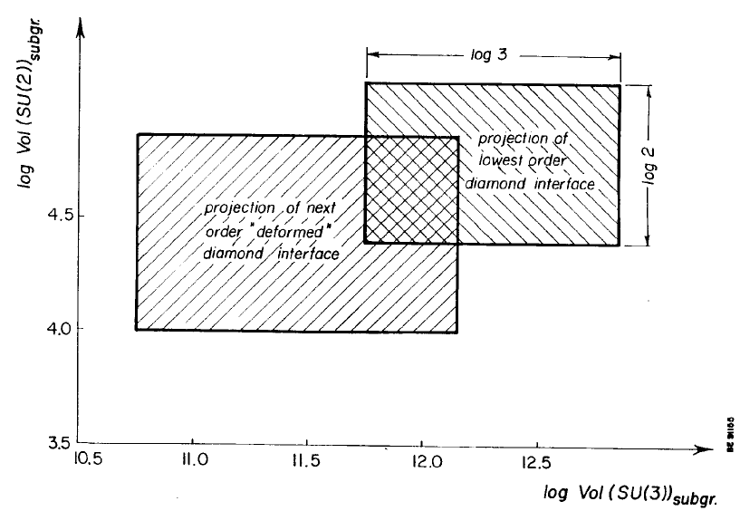
11.3 Appendix: Correction for non-commutativity in $\langle S_{act.,\;Coul}\rangle$

In the lowest order approximation we used simple vector addition as the rule of composition for Lie algebra vectors for non-Abelian groups. The correct rule of composition (to next to lowest order) for Lie algebra vectors corresponding to non-Abelian group multiplication yields a deviation in the distribution of plaquette variables that was obtained by convoluting link variable distributions. For a plaquette variable composed of a number $m$ (typically $m=3$) of active link variables, we need the distribution of the convolution of $m$ link variables in terms of Lie algebra elements corresponding to non-Abelian addition; this kind of addition, hereafter designated with the symbol +’ , leads to vector sums denoted with the notation $\mbox{\bf{P'}}=\sum^{\prime}_{r}\mbox{\bf{A}}_{r}=\mbox{\bf{A}}_{1}+^{\prime}\mbox{\bf{A}}_{2}+^{\prime}\cdots+^{\prime}\mbox{\bf{A}}_{m}$. In particular, we are interested in the width of the distribution of plaquette variables corresponding to the Lie algebra element P’.

For $m=2$ we have the expansion (Baker-Campbell-Hausdorff formula):

$$\mbox{\bf{A}}_{1}+^{\prime}\mbox{\bf{A}}_{2}=\mbox{\bf{A}}_{1}+\mbox{\bf{A}}_{2}+1/2[\mbox{\bf{A}}_{1},\mbox{\bf{A}}_{2}]+1/12[\mbox{\bf{A}}_{1}-\mbox{\bf{A}}_{2},[\mbox{\bf{A}}_{1},\mbox{\bf{A}}_{2}]]$$ (390)

The analogous expression for $m>2$ is

$$\mbox{\bf{P'}}=\sum_{r}^{m}\mbox{\bf{A}}_{r}+1/2\sum_{r,s;r<s}^{m}[\mbox{\bf{A}}_{r},\mbox{\bf{A}}_{s}]+1/12\sum_{r,s}^{m}[\mbox{\bf{A}}_{r},[\mbox{\bf{A}}_{r},\mbox{\bf{A}}_{s}]]$$ (391)

(modulo a term with average zero).

where higher order terms and terms that vanish upon averaging over symmetric fluctuations are omitted.

For an arbitrary Cartan Killing form CK(.,.), there obtains

$$\langle CK(\mbox{\bf{P'}},\mbox{\bf{P'}})\rangle=\sum_{r}^{m}\langle CK(\mbox{\bf{A}}_{r},\mbox{\bf{A}}_{r})\rangle+(1/4-2/12)\sum_{r,s;r<s}^{m}\langle CK([\mbox{\bf{A}}_{r},\mbox{\bf{A}}_{s}],[\mbox{\bf{A}}_{r},\mbox{\bf{A}}_{s}])\rangle$$ (392)

$$=\sum_{r}^{m}\langle CK(\mbox{\bf{A}}_{r},\mbox{\bf{A}}_{r})\rangle+1/12\sum_{r,s;r<s}^{m}\langle CK([\mbox{\bf{A}}_{r},\mbox{\bf{A}}_{s}],[\mbox{\bf{A}}_{r},\mbox{\bf{A}}_{s}])\rangle$$

Assuming the same Gaussian distribution for all the Lie algebra elements $\mbox{\bf{A}}_{r}$, the sum $\sum_{r,s;r<s}\langle CK([\mbox{\bf{A}}_{r},\mbox{\bf{A}}_{s}],[\mbox{\bf{A}}_{r},\mbox{\bf{A}}_{s}])\rangle$ in the last equation can be replaced by $\frac{m(m-1)}{2}\langle CK([\mbox{\bf{A}}_{r},\mbox{\bf{A}}_{s}],[\mbox{\bf{A}}_{r},\mbox{\bf{A}}_{s}])\rangle$ ($r$ and $s$ now just two arbitrary, different active links in the plaquette) in which case

$$\langle CK(\mbox{\bf{P'}},\mbox{\bf{P'}})\rangle=\sum_{r}^{m}\langle CK(\mbox{\bf{A}}_{r},\mbox{\bf{A}}_{r})\rangle+\frac{m(m-1)}{24}\langle CK([\mbox{\bf{A}}_{r},\mbox{\bf{A}}_{s}],[\mbox{\bf{A}}_{r},\mbox{\bf{A}}_{s}])\rangle.$$ (393)

Let $\mbox{\bf{P}}_{1}$ and $\mbox{\bf{P}}_{2}$ stand for a couple of independently distributed stochastic Lie algebra-valued variables (assume $\langle\mbox{\bf{P}}_{1}^{2}\rangle\approx\langle\mbox{\bf{P}}_{2}^{2}\rangle$ and $\langle\mbox{\bf{P}}_{1}\mbox{\bf{P}}_{2}\rangle\approx 0$) distributed as $\sum_{r=1}^{m}\mbox{\bf{A}}_{r}$. We have that $m^{2}\langle CK([\mbox{\bf{A}}_{r},\mbox{\bf{A}}_{s}],[\mbox{\bf{A}}_{r},\mbox{\bf{A}}_{s}])\rangle=\langle CK([\mbox{\bf{P}}_{2},\mbox{\bf{P}}_{1}],[\mbox{\bf{P}}_{2},\mbox{\bf{P}}_{1}])\rangle.$ and Eqn. (393) can be written

$$<CK(\mbox{\bf{P'}},\mbox{\bf{P'}})>=<CK(\mbox{\bf{P}}_{1},\mbox{\bf{P}}_{1})>+\frac{(m-1)}{(24m)}\cdot<CK([\mbox{\bf{P}}_{2},\mbox{\bf{P}}_{1}],[\mbox{\bf{P}}_{2},\mbox{\bf{P}}_{1}])>.$$ (394)

Rewrite the last factor in (394) as

$$\langle CK([\mbox{\bf{P}}_{2},\mbox{\bf{P}}_{1}],[\mbox{\bf{P}}_{2},\mbox{\bf{P}}_{1}])\rangle=-\langle CK(\mbox{\bf{P}}_{1},[\mbox{\bf{P}}_{2},[\mbox{\bf{P}}_{2},\mbox{\bf{P}}_{1}]])\rangle=-\langle CK(\mbox{\bf{P}}_{1},(\mbox{ad}\mbox{\bf{P}}_{2})^{2}\mbox{\bf{P}}_{1})\rangle$$ (395)

where we have used the invariance of the Cartan-Killing form under cyclic permutations of the arguments and the definition of $(\mbox{ad}\mbox{\bf{P}}_{2})^{2}$. Note that the operator $\langle(\mbox{ad}\mbox{\bf{P}}_{2})^{2}\rangle$ is invariant under similarity transformations by a group element $U$ in the adjoint representation:

$$\rho_{adj.\;rep.}(U)(\mbox{ad}\mbox{\bf{P}}_{2})^{2}\rho_{adj.\;rep}(U)^{-1}=(\mbox{ad}\mbox{\bf{P}}_{2})^{2}$$ (396)

To see this, combine Eqns. (368) and (370) to get

$$(((\mbox{ad}\mbox{\bf{P}}_{2})^{2})_{ij}=(\mbox{ad}(\mbox{\bf{X}}_{b})\mbox{ad}(\mbox{\bf{X}}_{c}))_{ij}P_{2,\;b}P_{2,\;c}.$$ (397)

Recall however that $\langle CK([\mbox{\bf{P}}_{2},\mbox{\bf{P}}_{1}],[\mbox{\bf{P}}_{2},\mbox{\bf{P}}_{1}])\rangle$ involves an average that insures that $\langle P_{2,\;b}P_{2,\;c}\rangle=\frac{\langle P^{2}_{2,\;a}\rangle}{d}\delta_{bc}$ in which case we have

$$\langle CK(\mbox{\bf{P}}_{1},(\mbox{ad}\mbox{\bf{P}}_{2})^{2}\mbox{\bf{P}}_{1})\rangle=\langle CK(\mbox{\bf{P}}_{1},P_{2,\;a}^{2}(\mbox{ad}(\mbox{\bf{X}}_{a}))^{2}\mbox{\bf{P}}_{1})\rangle$$ (398)

But $\frac{1}{d}P_{2,\;a}^{2}((\mbox{ad}(\mbox{\bf{X}}_{a}))^{2})$ is just the Casimir operator for the adjoint representation and therefore, by Schur’s Lemma, just proportional to the identity 1. This in turn means that we can write

$$\langle CK([\mbox{\bf{P}}_{2},\mbox{\bf{P}}_{1}],[\mbox{\bf{P}}_{2},\mbox{\bf{P}}_{1}])\rangle_{{{}_{\mbox{\scriptsize\bf{P}}}}_{1},\;{{}_{\mbox{\scriptsize\bf{P}}}}_{2}}=-\frac{\langle(\mbox{ad}\mbox{\bf{P}}_{2})^{2}\rangle_{{{}_{\mbox{\scriptsize\bf{P}}}}_{2}}}{\mbox{\bf{1}}}\langle CK(\mbox{\bf{P}}_{1},\mbox{\bf{P}}_{1})\rangle_{{{}_{\mbox{\scriptsize\bf{P}}}}_{1}}$$ (399)

where $\langle\cdots\rangle_{{{}_{\mbox{\scriptsize\bf{P}}}}_{1},\;{{}_{\mbox{\scriptsize\bf{P}}}}_{2}}$ denote averages w. r. t. both $\mbox{\bf{P}}_{1}$ and $\mbox{\bf{P}}_{2}$ whereas $\langle\cdots\rangle_{{{}_{\mbox{\scriptsize\bf{P}}}}_{1}}$ and $\langle\cdots\rangle_{{{}_{\mbox{\scriptsize\bf{P}}}}_{2}}$ denote respectively averages w. r. t. just $\mbox{\bf{P}}_{1}$ and just $\mbox{\bf{P}}_{2}$. Eqn. (394) becomes

$$<CK(\mbox{\bf{P'}},\mbox{\bf{P'}})>=<CK(\mbox{\bf{P}}_{1},\mbox{\bf{P}}_{1})>(1-\frac{(m-1)}{24m}\frac{\langle(\mbox{ad}\mbox{\bf{P}}_{2})^{2}\rangle_{{{}_{\mbox{\scriptsize\bf{P}}}}_{2}}}{\mbox{\bf{1}}})$$ (400)

$$<CK(\mbox{\bf{P'}},\mbox{\bf{P'}})>=<CK(\mbox{\bf{P}}_{1},\mbox{\bf{P}}_{1})>(1-\frac{(m-1)}{24m}\langle Tr_{adj.\;rep.}((\mbox{ad}\mbox{\bf{P}}_{2})^{2})/d\rangle_{{{}_{\mbox{\scriptsize\bf{P}}}}_{2}})$$

where $d$ is the dimension of the representation.

As we have defined squared distances as the Cartan-Killing form defined in terms of the defining representation:

$$dist^{2}(\mbox{\bf{1}},exp(\mbox{\bf{P}}_{2}))=-Tr_{def.\;rep.}(\mbox{\bf{P}}_{2},\mbox{\bf{P}}_{2})$$ (401)

we can rewrite Eqn.(400) as

$$\langle Tr_{def.\;rep.}(\mbox{\bf{P'}},\mbox{\bf{P'}})\rangle=\langle Tr_{def.\;rep.}(\mbox{\bf{P}}_{1},\mbox{\bf{P}}_{1})\rangle(1-\frac{(m-1)}{24m}\cdot\frac{2N}{d}\langle Tr_{def.\;rep.}(\mbox{\bf{P}}_{2},\mbox{\bf{P}}_{2})\rangle)$$ (402)

where we have used the result (373) for $SU(N)$ groups that

$$Tr_{adj.\;rep.}(\mbox{\bf{P}}_{2},\mbox{\bf{P}}_{2})=2N\mbox{Tr}_{def.\;rep.}(\mbox{\bf{P}}_{2},\mbox{\bf{P}}_{2})$$ (403)

Assuming (for Coulomb-like degrees of freedom) the distribution of Eqn. (163) for the link variables:

$$F(\sqrt{A^{2}/2})\propto\exp(-\tilde{\alpha}dist^{2}(1,\exp(\mbox{\bf{A}}))=\exp(\tilde{\alpha}\mbox{Tr}_{def.\;rep.}(\mbox{\bf{A}}^{2}))=\exp(-\frac{1}{2}\tilde{\alpha}A^{2}),$$ (404)

we have

$$-\langle\mbox{Tr}_{def.\;rep.}(\mbox{\bf{A}}_{r},\mbox{\bf{A}}_{s})\rangle=\delta_{rs}\frac{d}{2\alpha}.$$ (405)

For a plaquette consisting of $m$ active links, the corresponding result is

$$-\langle\mbox{Tr}_{def.\;rep.}(\mbox{\bf{P}}_{2},\mbox{\bf{P}}_{2})\rangle=\frac{md}{2\alpha}$$ (406)

From Eqn. (402) obtains

$$\frac{\langle\mbox{Tr}_{def.\;rep.}(\mbox{\bf{P'}},\mbox{\bf{P'}})\rangle}{\langle\mbox{Tr}_{def.\;rep.}(\mbox{\bf{P}},\mbox{\bf{P}})\rangle}=1+\frac{(m-1)}{24m}\cdot 2N\frac{m}{2\tilde{\alpha}\beta}$$ (407)

where we have used that $\tilde{\alpha}\stackrel{{\scriptstyle def.}}{{=}}\frac{\alpha}{\beta}$

Implementing the correction due to non-commutativity in the expression (167) for the convolution of $m=3$ link variables requires making the replacement

$$\frac{1}{\tilde{\alpha}}\rightarrow\frac{1}{\tilde{\alpha}}(1+\frac{m-1}{24m}\cdot 2N\frac{m}{2\tilde{\alpha}\beta})$$ (408)

This in turn means that the contribution to $``-\beta F"_{per\;active\;link}$ coming from $\langle S_{act.,\;Coul.}\rangle$ (Eqn.(175)) is modified as follows:

$$-2\sum_{i\in``Coul."}d_{i}\frac{3}{2\tilde{\alpha}_{i}}\rightarrow-2\sum_{i\in``Coul."}d_{i}\frac{3(1+\frac{m-1}{24m}\cdot 2N_{i}\cdot\frac{m}{2\tilde{\alpha}\beta})}{2\tilde{\alpha}_{i}}$$ (409)

It is sufficiently accurate to assume that the extremum w. r. t. $\tilde{\alpha}$ is the same as for the lowest order calculation: $\tilde{\alpha}_{i}=2m$ for all $i$.

For $m=3$, the correction for non-commutativity in $``-\beta F"\mid_{Coul.}$ is:

$$-2\sum_{i\in``Coul."}d_{i}\frac{3}{2\cdot 2m}\frac{(m-1)}{24m}\cdot 2N_{i}\frac{m}{2m\beta_{i}}=-\sum_{i\in``Coul."}\frac{d_{i}N_{i}}{144\beta_{i}}$$ (410)

Taking this correction into account in Eqn. (387) leads to

$$log\left(\frac{(\pi/6)^{dim(SMG)/2}}{Vol(SMG)}\right)-\sum_{i\in``Coul."}\frac{d_{i}N_{i}}{144\beta_{i}}=2log\left(\frac{\pi^{dim(SMG)/2}}{(1+\frac{2}{12\beta_{2}})^{3/2}(1+\frac{3}{12\beta_{3}2})^{8/2}Vol(SMG)}\right)$$ (411)

When both corrections - i.e., the correction for the Haar measure and the correction for non-commutativity in calculating $\langle S_{act.,\;Coul.}\rangle$ - are included, the defining condition for the phase boundary separating the totally Coulomb and totally confined phases becomes

$$\log Vol(SMG)=\log(6\pi)^{6}-\underbrace{\frac{1}{2\beta_{2}}-\frac{2}{\beta_{3}}}_{\mbox{Haar measure}}+\underbrace{\frac{1}{24\beta_{2}}+\frac{1}{6\beta_{3}}}_{\mbox{non-commutativity}}$$ (412)

While the sign of the correction to $\langle S_{act.,\;Coul.}\rangle$ for non-commutativity tends to compensate the correction for the Haar measure correction, the latter dominates in magnitude.

11.4 Appendix: Interaction terms in the action

It is illustrative to point out that the non-generic multi-critical point we get using the three parameters $\beta_{1},\beta_{N},\xi$ is an approximation that presupposes that there are no interaction terms of the type (132) in the physical action we seek to approximate. If such terms were present in the action of Nature, we could introduce a fourth parameter $\gamma$ as a coefficient to an action contribution that could compensate for interaction terms of the type (132). It is interesting to briefly consider how the presence of such interaction terms preclude a multi-critical point by explicitly introducing such a term. To this end, consider a term of the form

$$\gamma dist^{2}(\mbox{\bf{1}},U_{U(1)}(\Box))dist^{2}(\mbox{\bf{1}},U_{SU(N)}(\Box))\;\;\;\;(U_{U(1)}(\Box)\in U(1),\;U_{SU(N)}(\Box)\in SU(N))..$$ (413)

which is a slightly special case of (132).

If, for example, we consider the $SU(2)$ degrees of freedom, it is seen that the presence of this $\gamma$-term leads to an increase in the effective inverse squared coupling for the $SU(N)$ degrees of freedomby a quantity depending on $dist^{2}(\mbox{\bf{1}},U_{U(1)}(\Box))$:

$$\beta_{SU(N),\;eff.}=\beta_{SU(N)}+dist^{2}(\mbox{\bf{1}},U_{U(1)}(\Box)).$$ (414)

An analogous argument applies to the U(1) degrees of freedom:

$$\beta_{U(1),\;eff.}=\beta_{U(1)}+dist^{2}(\mbox{\bf{1}},U_{SU(N)}(\Box)).$$ (415)

The presence of such terms precludes a factorisation of the free energy. Equivalently, (127) is invalidated by such interaction terms. We can also reformulate the factorisation property (127) as an entropy additivity property. In this completely equivalent but perhaps more intuitive formulation, the condition for having the type of (non-generic) multiple points that we consider is that the total entropy is additive in entropy contributions from the “constituent” invariant subgroups. The additivity requirement for the entropy essentially means that the distribution of gauge degrees of freedom within the cosets of a factor group is the same for all the cosets of such a factor group.

The Entropy Formulation

Assuming the validity of the weak coupling approximation, we consider first distributions obtained from the exponentiated Manton action: $e^{\beta dist^{2}({\mbox{\scriptsize\bf{1}}},U_{l})}/Z$ ($l\in L\subseteq G$) where $dist^{2}(\mbox{\bf{1}},l)$ is the squared distance from the identity 1 to the group element $l$. If $l\in L$ is a coset of a factor group - i.e., if $L=G/H$ where $G$ is the gauge group and $H\triangleleft G$ - the function $dist^{2}$ is rendered unambiguous (for weak coupling) by requiring that the element $g\in G$ such that $gH=l\in G/H$ is generated alone by the Lie algebra of $G/H$. Such a distribution is a single normalised Gauss of width $(2\beta)^{-(dim(L))/2}$ centred at the group identity. We introduce the symbol $Gauss_{\beta}(l)$ as the designation of such a single-peaked distribution of plaquette variables $l$ that is centred at the identity. Bianchi identities are ignored. For the distribution $Gauss_{\beta}(l)$, the quantity $Vol(L)$ is the subgroup (or factor group) volume with the inverse squared couplings absorbed: $Vol(L)\stackrel{{\scriptstyle def.}}{{=}}\beta^{\frac{dim(L)}{2}}vol(L)$ where $vol(L)$ is the volume of $L$. This coincides with the definition of $Vol(L)$ as the group volume measured in units proportional to the fluctuation volume:

$$Vol(L)=\frac{vol(L)}{``fluctuation\;volume"}(\pi e)^{dim(L)/2}$$

The $Vol(L)$ are well defined in terms of the entropy if the distribution is additive in entropy contributions from the “constituent” invariant subgroups. Using the normalised plaquette distribution for a single plaquette (ignoring Bianchi identities)

$$Gauss_{\beta}(l)\stackrel{{\scriptstyle def}}{{=}}\frac{e^{-\beta dist^{2}({\mbox{\scriptsize\bf{1}}},l)}}{(\frac{\pi}{\beta})^{\frac{dim(L)}{2}}\cdot\frac{1}{vol(L)}}\;\;\;\;(l\in L),$$ (416)

the entropy can then be calculated as:

$$S_{entropy,\;Gauss_{\beta}}=\langle-\log Gauss_{\beta}(l)\rangle_{Gauss_{\beta}}=\langle-\log(\frac{\exp(-\beta dist^{2}(\mbox{\bf{1}},l))}{(\frac{\pi}{\beta})^{(dim(L))/2}\cdot\frac{1}{vol(L)}})\rangle$$

$$=-\log((\frac{\beta}{\pi})^{(dim(L))/2}vol(L))+\langle\beta dist^{2}(\mbox{\bf{1}},l)\rangle$$

$$=-\frac{dim(L)}{2}(\log(\frac{\beta}{\pi})-1)-\log vol(L)$$

$$=\frac{dim(L)}{2}\log(\frac{e\pi}{\beta})-\log vol(L)$$

$$S_{ent}=\frac{dim(L)}{2}\log(e\pi)-\log Vol(L).$$

The quantity $Vol(L)$ can be expressed in terms of the entropy $S_{entropy}$ as

$$Vol(L)=e^{-S_{entropy}}\cdot(e\pi)^{\frac{dim(L)}{2}}.$$ (417)

As the quantity $Vol(L)$ is the group volume measured in units of the fluctuation volume determined on the basis of a single Gauss distributed peak $Gauss_{\beta}(l)$ centred at the identity, we append $Gauss_{\beta}$ as a subscript to the quantity $Vol(L)$. Hence, (417) is rewritten

$$Vol_{Gauss_{\beta}}(L)=e^{-S_{entropy,\;Gauss_{\beta}}}\cdot(e\pi)^{\frac{dim(L)}{2}}.$$ (418)

For illustrative purposes, let us write down the entropy in the case of the $U(N)$ group when the distribution is given by the modified Manton action. By this is meant a distribution that, in addition to having a narrow maximum at the unit element 1, also can have narrow maxima at nontrivial elements of the discrete $\mbox{\bf{Z}}_{N}$ subgroups $\mbox{\bf{Z}}_{2}$ and $\mbox{\bf{Z}}_{3}$ inasmuch as we only consider $U(2)$ and $U(3)$ (these are the $U(N)$ groups relevant for the $SMG$). Having now the possibility of these subsidiary peaks, we supplement the parameters $\beta_{U(1)}$ and $\beta_{SU(N)}$ with a parameter $\xi^{(p)}$. The parameter $\xi^{(p)}$ specifies the height of the subsidiary maxima centred at nontrivial elements $p\in\mbox{\bf{Z}}_{N}$ relative to the maximum in the distribution that is centred at the group identity 1. In the approximation that there are no interaction terms in the action, it is then possible to have non-generic multiple points in a $3$-dimensional action parameter space spanned by the variables

$$(\beta_{U(1)}^{(p)},\beta_{SU(N)}^{(p)},\xi^{(p)}).$$ (419)

where the superscript $p$ labels the element $p\in\mbox{\bf{Z}}_{N}$ to which the parameters pertain. This set of three parameters determines a distribution $\frac{e^{S_{mod.\;Manton}}}{Z}$ on the group $U(N)$ ($N=2$ or $3$) in the neighbourhood of the element $p\in\mbox{\bf{Z}}_{N}\subset U(N)$.

As we only need to consider the local structure of the gauge group, we can decompose a $U(N)$ plaquette variable $U_{U(N)}(\Box)$ into a $U(1)$ part and a $SU(N)$ part: $U_{U(N)}(\Box)=(U_{U(1)}(\Box),U_{SU(N)}(\Box))$.

For $U(\Box)$ near the element $p\in\mbox{\bf{Z}}_{N}$ ($N=2$ or $3$), the distribution $\frac{e^{S_{mod.\;Manton}}}{Z}$ is dominated by the Gauss function

$$Gauss_{(\xi^{(p)},\beta^{(p)}_{U(1)},\beta^{(p)}_{SU(N)})}(U(\Box))\stackrel{{\scriptstyle def}}{{=}}$$ (420)

$$\frac{\exp(\beta^{(p)}_{U(1)}\;dist^{2}(p,U_{U(1)}(\Box)))\cdot\exp(\beta^{(p)}_{SU(N)}\;dist^{2}(p,U_{SU(N)}(\Box)))}{Z}$$

where $(2\beta_{U(1)}^{(p)})^{\frac{1}{2}}$ respectively $(2\beta_{SU(N)}^{(p)})^{\frac{1}{2}}$ is the width of the maximum along the $U(1)$ and the $SU(N)$ direction(s) of the maximum centred at $p\in\mbox{\bf{Z}}_{N}$. The are $N$ such Gauss-shaped maxima in the distribution $\exp(S_{mod.Man.}(U(\Box)))/Z$ when $U(\Box)\in U(N)$; $\xi^{(p)}$ is the height of the maximum at $p\in\mbox{\bf{Z}}_{N}$ relative to the height of the Gauss-shaped maximum centred at the identity. The latter maximum is denoted $Gauss_{(1,\beta_{U(1)}^{({\mbox{\scriptsize\bf{1}}})},\beta_{SU(N)}^{({\mbox{\scriptsize\bf{1}}})})}U(\Box)$. The partition function $Z$ that normalises the $N$-maxima ($N=2$ or $3$) modified Manton distribution $\exp(S_{mod.Man.})/Z$ is

$$Z=\frac{\pi^{N^{2}/2}}{vol(U(1))vol(SU(N))}\left(\frac{1}{(\beta_{U(1)}^{({\mbox{\scriptsize\bf{1}}})})^{\frac{1}{2}}(\beta_{SU(N)}^{({\mbox{\scriptsize\bf{1}}})})^{\frac{N^{2}-1}{2}}}+\frac{N-1}{(\beta_{U(1)}^{(p)})^{\frac{1}{2}}(\beta_{SU(N)}^{(p)})^{\frac{N^{2}-1}{2}}}\right)$$ (421)

It is easy to show that $\beta^{(p)}=\beta^{({\mbox{\scriptsize\bf{1}}})}/\xi^{(p)}$ if we let $\beta^{(p)}$ be defined by

$$e^{\beta^{(p)}dist^{2}(p,U(\Box))}=\xi^{(p)}e^{\beta^{({\mbox{\scriptsize\bf{1}}})}dist^{2}({\mbox{\scriptsize\bf{1}}},U(\Box))}.$$ (422)

The partition function can now be written

$$Z=\frac{\pi^{N^{2}/2}}{(\beta_{U(1)}^{({\mbox{\scriptsize\bf{1}}})})^{\frac{1}{2}}(\beta_{SU(N)}^{({\mbox{\scriptsize\bf{1}}})})^{\frac{N^{2}-1}{2}}vol(U(1))vol(SU(N))}(1+\xi^{N^{2}}(N-1))$$ (423)

For completeness we write down the distribution function for the modified Manton action:

$$\frac{e^{S}_{mod.\;Manton}}{Z}=$$ (424)

$$\left\{\begin{array}[]{ll}Gauss_{(1,\beta_{U(1)}^{({\mbox{\scriptsize\bf{1}}})},\beta_{SU(N)}^{({\mbox{\scriptsize\bf{1}}})})}U(\Box)&\mbox{if $U_{U(1)}(\Box),U_{SU(N)}(\Box)$ near identity of $U(N)$}\\ Gauss_{(\xi^{(p)},\beta^{({\mbox{\scriptsize\bf{1}}})}_{U(1)}/(\xi^{(p)})^{2},\beta_{SU(N)}^{({\mbox{\scriptsize\bf{1}}})}/(\xi^{(p)})^{2})}(U(\Box))&\mbox{if $U_{U(1)}(\Box),U_{SU(2)}(\Box)$ near nontrivial element of $\mbox{\bf{Z}}_{N}$}\\ 0&\mbox{if $U_{U(1)}(\Box),U_{SU(2)}(\Box)$ not near any element of $\mbox{\bf{Z}}_{N}$}\end{array}\right.$$

It is of course to be understood the $p\in\mbox{\bf{Z}}_{N}$ is chosen so as to minimise $dist^{2}(p,U(\Box))$ ($U(\Box)\in U(N)$). We have in mind a weak coupling approximation which implies that the distribution $e^{S}_{mod.\;Manton}/Z$ is only appreciable near the elements of $Z_{N}$ so at any place in the group, at most one Gaussian peak contributes to a non-vanishing value of the distribution. With this restriction there is no ambiguity in talking about the squared distance between group elements.

The distribution (424) is normalised w.r.t the Haar measure. Recall that the quantity $Vol(L)$ is the volume of the subgroup (or factor group $L$) measured in units of the fluctuation volume. Note however that in the case of the modified Manton action, the unit of volume for $Vol(L)$ is the sum of the fluctuation volumes of several Gauss distributions that, in addition to a distribution centred at the identity, can also include distributions centred at nontrivial elements $p=e^{\pm i2\pi/N}\mbox{\bf{1}}\;\;(N=2,3)$ of $Z_{N}$ subgroups having height $\xi$ and width $(2\beta^{(p)})^{\frac{1}{2}}=(\frac{2\beta^{({\mbox{\scriptsize\bf{1}}})}}{(\xi^{(p)})^{2}})^{\frac{1}{2}}$. This is sometimes indicated explicitly by writing $Vol(L)$ using the notation $Vol_{Gauss_{(\xi^{(p)},\beta^{(p)}_{U(1)},\beta^{(p)}_{SU(N)}})}$.

The entropy of the distribution (424) is

$$S_{entropy}\stackrel{{\scriptstyle def}}{{=}}-\langle\frac{e^{S}_{mod.\;Manton}}{Z}\rangle=-\frac{1}{1+(N-1)\xi}\langle\log\frac{Gauss_{(1,\beta^{({\mbox{\scriptsize\bf{1}}})}_{U(1)},\beta^{({\mbox{\scriptsize\bf{1}}})}_{SU(N)})}}{1+(N-1)\xi}\rangle-$$ (425)

$$-\frac{(N-1)\xi}{1+(N-1)\xi}\langle\log\frac{\xi(Gauss_{(p,\beta_{U(1)}^{(p)},\beta_{SU(N)}^{(p)})}}{1+(N-1)\xi}\rangle-$$

$$=-\frac{1}{1+(N-1)\xi}\log(\frac{1}{1+(N-1)\xi})-\frac{(N-1)\xi}{1+(N-1)\xi}\log(\frac{\xi^{(N^{2}+1)}}{1+(N-1)\xi})-$$

$$-\langle\log Gauss_{(1,\beta_{U(1)}^{{\mbox{\scriptsize\bf{1}}}},\beta_{SU(N)}^{{\mbox{\scriptsize\bf{1}}}})}\rangle$$

where we have used that $Gauss_{(p,\beta_{U(1)}^{(p)},\beta_{SU(N)}^{(p)})}=\xi^{N^{2}}Gauss_{1,\beta_{U(1)}^{({\mbox{\scriptsize\bf{1}}})},\beta_{SU(N)}^{({\mbox{\scriptsize\bf{1}}})})}$.

Rearranging yields

$$S_{entropy}=$$ (426)

$$\underbrace{-\log(\frac{1}{1+(N-1)\xi}\cdot(\xi)^{\frac{(N^{2}+1)(N-1)\xi}{1+(N-1)\xi}})}_{S_{entropy,\;{\mbox{\scriptsize\bf{Z}}}_{N}}}-$$

$$-\underbrace{\langle\log Gauss_{(1,\beta_{U(1)}^{({\mbox{\scriptsize\bf{1}}})})}\rangle}_{S_{entropy,\;Gauss_{(1,\beta^{({\mbox{\scriptsize\bf{1}}})}_{U(1)})}}}-$$

$$-\underbrace{\langle\log Gauss_{(1,\beta_{SU(N)}^{({\mbox{\scriptsize\bf{1}}})})}\rangle}_{S_{entropy,\;Gauss_{(1,\beta^{({\mbox{\scriptsize\bf{1}}})}_{SU(N)})}}}-$$

The quantity $S_{entropy,\,{\mbox{\scriptsize\bf{Z}}}_{N}}$ is the entropy due to presence of the discrete Gaussian peaks at the elements of $\mbox{\bf{Z}}_{N}$. The quantities $S_{entropy,\;Gauss(1,\beta_{U(1)})}$ and $S_{entropy,\;Gauss(1,\beta_{SU(N)})}$ are the entropies due respectively to fluctuations of (average) widths $(2\beta_{1})^{-1/2}$ and $(2\beta_{N})^{-1/2}$ within the Gaussian peaks situated at the identity.

We have shown that the distribution (424) defined on the non-simple group $U(N)\;\;(N=2$ or $3)$ has the property that

$$S_{entropy}=S_{entropy,\;{\mbox{\scriptsize\bf{Z}}}_{N}}+S_{entropy,\;Gauss_{(1,\beta_{U(1)})}}+S_{entropy,\;Gauss_{(1,\beta_{SU(N)})}}.$$ (427)

We refer to this property as “entropy additivity”. In the absence of interactions between the degrees of freedomof the constituent invariant subgroups, the distribution (424) defined on $U(N)$ by the three parameters $\beta^{(p)}_{U(1)},\beta^{(p)}_{SU(N)},$ and $\xi^{(p)}$ has this property and the $U(N)$ phase diagram spanned by these three parameters has a non-generic multiple point at which $5$ phases convene.

In order to construct the phase diagram for $U(N)$ we equate the free energies (137) using the ansatz corresponding respectively to confinement w. r. t. $H_{1}$ and $H_{2}$. This yields

$$\frac{Vol(H_{1})}{Vol(H_{2})}=(6\pi)^{\frac{dim(H_{1})-dim(H_{2})}{2}}$$ (428)

as the condition to be fulfilled at the phase boundary separating a phase confined w. r. t. $H_{1}$ from a phase confined w. r. t. $H_{2}$.

For distributions such as (424) that, in addition to peaks at the group identity, also have peaks at nontrivial elements of discrete invariant subgroups, we can now write down an expression for $Vol(L)$ in terms of the entropy. By analogy to (418), we have, for example, for $L=SU(N)/\mbox{\bf{1}}$

$$Vol(SU(N)/\mbox{\bf{1}})=e^{-S_{entropy,\;Gauss_{(1,\beta^{({\mbox{\scriptsize\bf{1}}})}_{SU(N)})}}-S_{entropy,\;{\mbox{\scriptsize\bf{Z}}}_{N}}}\cdot(e\pi)^{\frac{N^{2}-1}{2}}$$ (429)

$$=Vol_{Gauss_{(1,\beta_{SU(N)})}}(SU(N))\cdot e^{-S_{entropy,\;{\mbox{\scriptsize\bf{Z}}}_{N}}}$$

$$=\beta_{N}^{\frac{N^{2}-1}{2}}vol(SU(N)\cdot\frac{1}{1+(N-1)\xi}\cdot(\xi)^{\frac{(N^{2}+1)(N-1)\xi}{1+(N-1)\xi}}$$

where we have used (418) and (426) in the final step.

Figure 25: Action terms of the type (413) give rise to interactions in the sense that the distribution of group elements within cosets varies along the distribution of cosets.

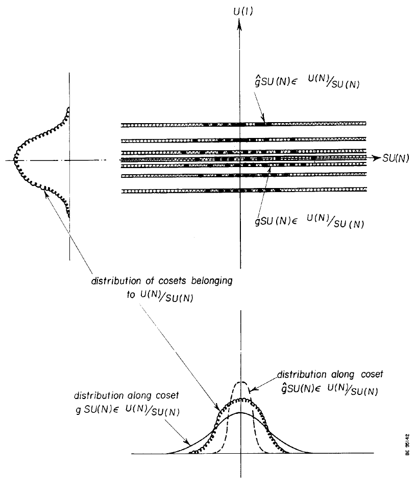
Returning now to the discussion of interaction terms in the action of the type (413) that give rise to effective inverse squared couplings of the types (414) and (415), we briefly argue that if the coefficient $\gamma$ of such an interaction term (413) is large, the entropy is not (approximately) additive in contributions from the constituent invariant subgroups. Moreover, a consequence of this is that there is no approximate multi-critical point in the three-parameter space spanned by $\beta^{(p)}_{U(1)},\;\beta^{(p)}_{SU(N)},$ and $\xi^{(p)}$. To illustrate this, we consider again the phase boundaries involving degrees of freedomisomorphic with the $SU(N)$.

One of these phase boundaries, defined by the condition $Vol(U(N)/U(1))=(6\pi)^{(N^{2}-1)/2)}$, separates the totally confining phase from the phase with confinement w. r. t. $U(1)$. The quantity $Vol(U(N)/U(1)$ is well defined because the the distribution of cosets belonging to the factor group $U(N)/U(1)$ has a well defined width and thereby a well defined entropy.

The other phase boundary defined by a condition on the $SU(N)$ degrees of freedomis that separating the phase with confinement w. r. t. $SU(N)$ from the phase having confinement only w. r. t. $\mbox{\bf{Z}}_{N}$. At this boundary, the condition to be fulfilled is $Vol(SU(N)/\mbox{\bf{Z}}_{N})=(6\pi)^{(N^{2}-1)/2}$. The quantity $Vol(SU(N)/\mbox{\bf{Z}}_{N})$ is determined as an average over the distributions of $SU(N)$ elements within cosets $gSU(N)\in U(N)/SU(N)$. We can use the restriction $g\in U(1)$ as we only want to use $g$ as a label for the cosets of $U(N)/SU(N)$. Unless $\gamma=0$, a distribution of $SU(N)$ elements within a coset $gSU(N)$ will depend on $g\in U(1)$. Hence the quantity $Vol(SU(N)/\mbox{\bf{Z}}_{N})$ is calculated as an average (with weights given by the distribution of cosets $gSU(N)\in U(N)/SU(N)\stackrel{{\scriptstyle-}}{{\simeq}}U(1)$) of $SU(N)$ distributions that, for $\gamma\not=0$, are different for each coset $gSU(N)$. The calculation of $Vol(SU(N)/\mbox{\bf{Z}}_{N})$ depends therefore on the distribution of the cosets $gSU(N)\in U(N)/SU(n)$. Only if $\gamma=0$ is the distribution of $SU(N)$ degrees of freedomwithin each coset $gSU(N)\in U(N)/SU(N)$ the same. In this case one obtains the same result for $Vol(U(N)/\mbox{\bf{Z}}_{N})$ for all distributions of the cosets of the factor group $U(N)/SU(N)$ that coincides with the value of $Vol(U(N)/U(1))$ at a non-generic multi-critical point.

A similar line of reasoning applies to the $U(1)$ degrees of freedom. For both the $U(1)$ and the $SU(N)$ degrees of freedom, we can say that an action with $\gamma=0$ leads to a distribution of the group that is “entropy-additive” because the widths of the distributions of $U(1)$ and $SU(N)$ elements within respectively the cosets and $gSU(N)\in U(N)/SU(N)\;\;(g\in U(1))$ $hU(1)\in U(N)/U(1)\;\;(h\in SU(N))$ are the same for all displacements $g$ and $h$.

11.5 Appendix: Proposed model for the stability of the multiple point

We propose a mechanism for the stability of the multiple point that is based on a model which could be called a “nonlocal gauge glass model”. which is very much inspired by the project of “random dynamics[8, 29, 26]”.ese two assumptions - multiple point criticality and degenerate vacua differing by a quantity of order unity in Planck units - leads to The essential feature is the influence of a bias effect that can occur in the presence of a plaquette (or multi-plaquette) action the functional form of which is taken to be quenched random. This could mean that for each Wilson loop $\Gamma$, the coefficients (called the “$\beta$’s”) in say a character expansion of the Wilson loop action are fixed at the outset as random values and remain fixed during the evaluation of the functional integral. While translational invariance is broken at least at small scales because a different set of random $\beta$’s is associated with each Wilson loop, it is presumably regained at least approximately in going to large distances inasmuch as it is assumed that the statistical distribution of quenched random variables is translation-ally invariant.

Randomly weighted terms in the action from the different Wilson loops would on the average contribute nothing to the inverse squared coupling were it not for the bias: the vacuum dominant value of a Wilson loop variable (a point in the gauge group) is correlated with the values of the quenched random coefficients for the Wilson loop under consideration. This correlation comes about because the vacuum field configuration adjustments resulting from the tendency to approximately maximise the exponential of the action $\exp(S)$ as a function of link variables will concurrently tend to make the second derivative w. r. t. Wilson loop variables of $\exp(S)$ more negative.

In the simplest model, the gauge glass we use is rather strongly nonlocal because we assume that the quenched random contributions to the action are not restricted to contributions from elementary plaquettes, but in principle include all Wilson loops. If this should lead to problems with locality, we can postulate that only loops up to some finite size are present in the action since the most crucial prerequisite for the bias mechanism is the inclusion of many Wilson loops with the size distribution being of only secondary importance.

The bias effect can be formulated as an additional term in the Callan-Symanzik $\beta$-functions (in addition to the normal renormalization group contribution). To see this, envision a series of calculations of the effective couplings $g(\mu)$ for successively larger inverse energies $\mu^{-1}$. For each value of $\mu^{-1}$, Wilson loops of size up $\mu^{-1}$ are included in computing $g(\mu)$; therefore a calculation of $g(\mu)$ includes more and more Wilson loops in going towards the infrared. The inclusion of progressively longer and longer loops takes place in a background field made up of contributions from the already included smaller loops that are approximately described as a background continuum Lagrange density $-\frac{1}{4g^{2}(\mu)}F_{\mu\nu}^{2}$. This process, in which the coupling $g(\mu)$ becomes smaller and smaller the more loops it accounts for, culminates in $g(\mu)$ attaining the critical value whereupon the influence of additional loops on the vacuum configuration is drastically diminished because the transition to a $g(\mu)$ corresponding to the Coulomb phase leads to a vacuum configuration that is much less readily influenced than in the confinement phase. Contributions from larger Wilson loops are no longer correlated with the vacuum dominant field configuration that is almost solely determined by the Wilson loops of smaller spatial extent. Without the “protection” of the bias effect, the contributions from these larger loops cancel out on the average because of the assumed randomness in the signs of action terms with the result that the effective couplings will no longer be modified much by the inclusion of larger Wilson loops that show up in going to larger length scales.

The variation of the effective coupling due to the bias effect might formally be included in a generalised Callan-Symanzik $\beta$-function. (actually we mean a multicomponent vector of generalised $\beta$-functions with one component for each parameter of a single plaquette action of a course-grained lattice at the scale $\mu$). These generalised $\beta$-functions (i.e., the components of the vector of generalised $\beta$-functions) contain contributions that take into account that the part of the Lagrangian of the theory that is used to define gauge couplings $g(\mu)$ is changing as we go to larger length scales. That this change has a non-vanishing average effect on the couplings is due to the bias effect. These extra contributions to the $\beta$-functions, which are in addition to the normal renormalization group effects, make the generalised $\beta$-functions explicitly scale dependent. Specifically, we envision rapid variations of the $\beta$-functions as the bias effect is drastically weakened at the transition to a Coulomb-like phase. If the $\beta$-functions become zero, this would result in an infrared attractive fixed point near the phase transitions at the multiple point.

An important point is that multiple point criticality is implied by almost any mechanism that drives a gauge coupling to a critical value because a mechanism that seeks out the critical coupling for some gauge group will probably function in the same way for all invariant subgroups of a gauge group. But this is tantamount to seeking out the multiple point which by definition is the point or surface in the phase diagram at the borderline between confining and Coulomb phases for all invariant subgroups. In particular, our model as outlined above would, imply that Wilson loop contributions $\prod_{\;\mbox{\begin{picture}(4.15,10.0)\put(0.0,3.0){\circle*{2.0}} \put(0.0,2.75){\line(1,0){7.0}} \put(7.3,3.0){\circle*{2.0}}\mbox{ } \end{picture} }\;\in\Gamma}U(\mbox{\begin{picture}(4.15,10.0)\put(0.0,3.0){\circle*{2.0}} \put(0.0,2.75){\line(1,0){7.0}} \put(7.3,3.0){\circle*{2.0}}\mbox{ } \end{picture} })$ depending only on the cosets in $G/H$ w.r.t. some invariant subgroup $H$ would become very ineffective in bringing about a further increase in the inverse squared couplings (for the degrees of freedomcorresponding to the factor group) once it is only the invariant subgroup $H$ of the group $G$ that remains “confining”; in other words, the couplings for $G/H$ stop falling (in the crudest approximation) once $G/H$ “reaches the Coulomb phase”.

Several alternatives to the nonlocal gauge glass explanation for the stability of the multiple point (assuming it exists) have been considered. We have for example in previous work, prior to the advent of the principle of multiple point criticality, used the entropy as the quantity to be maximised in the predictions of gauge couplings from criticality. In this earlier work, we have for the non-Abelian Lie subgroups of the $SMG^{3}$ considered criticality only w.r.t. the Lie subgroups $SU(2)$ and $SU(3)$ and not for criticality w. r. t. the $\mbox{\bf{Z}}_{2}$ and $\mbox{\bf{Z}}_{3}$ discrete invariant subgroups of, respectively, $SU(2)$ and $SU(3)$. We found that the entropy, calculated to lowest order, was to first approximation constant on an interface of finite extent that separated the totally Coulomb-like and totally confinement phases in the parameter space of the $SMG$ phase diagram. In effect, this interface prohibited other partially confining phases from meeting at a multiple point. We now find that the addition of action parameters that also allow the discrete invariant subgroups to become critical results in the shrinking of this interface into a point that coincides with the multiple point. This can be expected to affect the entropy because, at the multiple point, we are also on the verge of confinement for the groups $\mbox{\bf{Z}}_{2}$ and $\mbox{\bf{Z}}_{3}$. This means that a small change in the appropriate action parameters can bring about a transition from a Coulomb-like phase to a confinement-like phase with the difference between the two being, for example, defined by the respective perimeter and area law decay of Wilson loops (for charges 1/2 or 1/3 in the case of $\mbox{\bf{Z}}_{2}$ and $\mbox{\bf{Z}}_{3}$ respectively).

In the action parameter space that includes parameters that can be adjusted so as to have criticality w. r. t. the discrete invariant subgroups $\mbox{\bf{Z}}_{2}$ and $\mbox{\bf{Z}}_{3}$, the entropy is constant to lowest order along a (hyper)surface separating the totally Coulomb from totally confined phases. But a calculation to next order appears to lead to the conclusion that the entropy is not maximum at the multiple point thereby obviating the idea of maximum entropy as an explanation for the multiple point.

However, it can be claimed that the multiple point is such a characteristic “corner” of the phase diagram that it is extremely likely that there is some relevant physical quantity or property that is extremised at this point. A possible scenario that might in part rescue the maximum entropy idea is that, at the multiple point, there are strong fluctuations along the discrete subgroup directions of the gauge group that, for given entropy, might be very effective in preventing potential Higgs fields from bringing the model into a Higgs phase. In other words, the entropy that comes from the “discretised” lack of knowledge (as to which element of the discrete invariant subgroups in the neighbourhood of which the plaquette variable takes a value) may function better in suppressing the tendency for “Higgsing” than the same amount of entropy arising from fluctuations within the individual Gaussian distributions $e^{S_{Manton}}$ centred at the elements of $\mbox{\bf{Z}}_{2}$ and $\mbox{\bf{Z}}_{3}$. If this were true, one might use Higgs suppression as the property to be optimised at the multiple point.

Yet another admittedly rather speculative approach to explaining the multiple point suggest that the functional integral for the partition function in baby universe theory should have a maximal value at the multiple point[44].

Meaningful continuum couplings for lattice gauge theories do not exist for couplings that exceed the critical values[100]. This is corroborated by the observation[100] that Mitrushkin[101] only formally obtains a strong continuum coupling in the Coulomb phase.

In summary, we have in this appendix supplemented the postulate of the principle of multiple point criticality with proposals as to how a stable Planck scale multiple point might be realized. To this end, we described a gauge glass model inspired by random dynamics. This model, which uses a quenched random action, has a bias causing weaker couplings that is discontinuously diminished at the multiple point. This leads to a zero of a generalised Callan-Symanzik $\beta$ function thereby establishing the multiple point as an approximate “infrared stable” fixed point.

The speculative nature of these arguments in no way detracts from the most important justification for the principle which is the noteworthy phenomenological success.

References

- [1] D.L. Bennett and H.B. Nielsen. Gauge Couplings Calculated from Multiple Point Criticality Yield : At Last the Elusive Case of . J. Mod. Phys A. (submitted 31 May, 1996), page 85 pages, 1996.
- [2] D.L. Bennett. Multiple Point Criticality and the Avoidence of Paradoxes in the Presence of Non-Locality in Physical Theories: A resume of discusions with H.B. Nielsen during the summer of 1995. Available from Forskningscenter for Livskvalitet, St. Kongensgade 70, DK-1264 Copenhagen as preprint nr. QLRC-95-2; coincides essentially with talk by D. Bennett: “Who’s Afraid of the Past” (given 8 August 1995 for the “Cross-Disciplinary Initiative” at the Niels Bohr Institute), September 1995. 23 pages.
- [3] D.L. Bennett and H.B. Nielsen. Predictions for Non-Abelian Fine Structure Constants from Multiple Point Criticality. Intl. J. Mod. Phys., A9:5155–5200, 1994.
- [4] D.L. Bennett and H.B. Nielsen. Constants of Nature from a Multiple Point Criticality Finetuning Mechanism: Predictions of Standard Model Gauge Couplings. In Sally Seidel, editor, The Albuquerque Meeting, The University of New Mexico, pages 1410–1415. Division of Particles and Fields ’94 Meeting of the Am. Phys. Soc., Albuquerque, 2-6 August 1994, World Science Pub. Co., Inc., Singapore, August 2-6 1994. Also available as preprint NBI-HE-95-45 from The Niels Bohr Institute.
- [5] D.L. Bennett, C.D. Froggatt, and H.B. Nielsen. Nonlocality as an Explanation for Finetuning in Nature. In D. Lüst and G. Weight, editor, Proc. XXXVIII International Symposium Ahrenshoop on the Theory of Elementary Particles, Wendish-Rietz, August 30-September 3 1994. Availible as preprint NBI-HE-95-07 from The Niels Bohr Institute.
- [6] D.L. Bennett, C.D. Froggatt, and H.B. Nielsen. Nonlocality as an Explanation for Finetuning and Field Replication in Nature. In Proceedings of the 7th Adriatic Conference ”Theoretical and experimental Perspectives in Particle Phenomenology”, Island of Briuni, September 13-20 1994. Available as preprint NBI-95-15 from The Niels Bohr Institute or GUPTA /95/04/1 from the University of Glasgow.
- [7] C.D. Froggatt and H.B. Nielsen. Origin of Symmetries. World Scientific Publishing Co., Singapore, 1991.
- [8] H.B. Nielsen. Field Theories Without Fundamental Gauge Symmetries. Phil. Trans. R. Soc. Lond., A310:261–272, 1983.
- [9] H.B. Nielsen. Dual Strings. In I.M. Barbour and A.T. Davies, editors, Proceedings of the XVII Scottish University Summer School in Physics: Fundamentals of Quark Models, page 528. University of Glasgow, 1976, St. Andrews, 1976. (see section on Catastrophe Theory).
- [10] H.B. Nielsen. Har vi brug for fundamentale naturlove (in Danish). Gamma 36, page 3, 1978.
- [11] H.B. Nielsen. Har vi brug for fundamentale naturlove (in Danish). Gamma 37, page 35, 1978.
- [12] D.L. Bennett, C.D. Froggatt, and H.B. Nielsen. Multiple Point Criticality, Fine Structure Constants and Mass Hierarchies. In Proceedings of the International Conference on High Energy Physics, July 1994. Availible as preprint NBI-HE-95-44 from The Niels Bohr Institute.
- [13] D.L. Bennett, H.B. Nielsen, and I. Picek. Number of Generations Related to Coupling Constants by Confusion. In Proceedings of the XX International Symposium Ahrenshoop on the Theory of Elementary Particles, page 383. Institut für Hochenergiphysik, Akad. der Wissenschaften der DDR, Berlin-Zeuthen, October 13-17 1986.
- [14] D.L. Bennett, H.B. Nielsen, and I. Picek. Gauge Group Replication as an Explanation for the Smallness of the Finestructure Constant. In E. Wieczorek, editor, Proceedings of the XXI International Symposium Ahrenshoop on the Theory of Elementary Particles, pages 287–308. Institut für Hochenergi Physik, Akademie der Wissenschaften der DDR, Berlin-Zeuthen, Sellin, October 12-16 1987.
- [15] H.B. Nielsen, D.L. Bennett, and I. Picek. An Inequality Relating Gauge Coupling Constants and the Number of Generations in a String Inspired Model. In Proceedings of the Beijing Workshop on String Theories. World Scientific, Singapore 1988, July 6 - Sept. 5 1987. presented in Beijing in November 1987 by H.B. Nielsen.
- [16] D.L. Bennett, H.B. Nielsen, and I. Picek. Understanding fine structure constants and three generations. Phys. Lett., B208:275–80, 1988.
- [17] H.B. Nielsen, D.L. Bennett, and I. Picek. Formulation Using Compactified Dimensions to get an Inequality Relating Coupling Constants and the Number of Generations. In Proceedings of the Workshop on Superstring Theory. Indian Institute of Technology, Kanpur, December 13-24 1987.
- [18] D.L. Bennett, H.B. Nielsen, and I. Picek. Understanding fine structure constants and three generations. In V.A. Petrov, editor, Proceedings of the XI Workshop on High Energy Physics and Field Theory, Protvino, pages 419–27. Academy of Sciences of the U.S.S.R., Moscow 1989, Nauka, Moscow 1989, July 5-9 1988.
- [19] L. Michel. Invariance in quantum mechanics and group extension. In F. Gürsey, editor, Group Theoretical Concepts and Methods in Elementary Particle Physics. Lectures of the Istanbul Summer School of Theoretical Physics, Gorden and Breach Science Publishers, July 16 - August 4 1962.
- [20] H.B. Nielsen and N. Brene. Gauge Glass. In Proceedings of the XVIII International Symposium on the Theory of Elementary Particles, Ahrenshoop. Institut für Hochenergiphysik, Akad. der Wissenschaften der DDR, Berlin-Zeuthen, 1985, 1984.
- [21] D.L. Bennett, N. Brene, L. Mizrachi, and H.B. Nielsen. Confusing the Heterotic String. Phys. Lett., B178:179–186, 1986.
- [22] G. Gaeta. Intl. J. Theor. Phys., 32:727, 1993.
- [23] S. Rajpoot. Some Consequences of Extending the SU(5) Gauge Symmetry to the Generation Symmetry . Phys. Rev., D24:1890–1894, 1981.
- [24] H.B. Kim and J.E. Kim. Coupling Constant Unification and LEP Data. preprint SNUTP-92-89, 1992. Center for Theoretical Physics and Department ofPhysics, Seoul National University, Seoul 151-742, Korea.
- [25] U. Amaldi and W. de Boer and H. Fürstenau. Comparison of grand unified theories with electroweak and strong coupling constants measured at LEP. Phys. Lett., B260:447–455, 1991.
- [26] D.L. Bennett, N. Brene, and H.B. Nielsen. Random dynamics. In L. Brink, R. Marnelius, J.S. Nilsson, P. Salomonson, and B. Skagerstam, editors, Proceedings of Nobel Symposium 67: Unification of Fundamental Interactions, Marstrand, Sweden, page 158. The Royal Swedish Academy of Sciences, 2-7 June 1986. Physica Scripta Vol. T15, 1987; Copublished by World Scientific Publishers, London (1988).
- [27] H.B. Nielsen. Lecture notes (QCD etc. 1993) and private communications.
- [28] D. Förster and H. B. Nielsen and M. Ninomiya. Phys. Lett., 94B:135, 1980.
- [29] H.B. Nielsen, D.L. Bennett, and N. Brene. The Random Dynamics Project. In J. Ambjørn and B.J. Durhuus and J.L. Petersen, editor, Recent Developments in Quantum Field Theory,. Proceedings of the Niels Bohr Centennial Conference, Copenhagen, North Holland, Amsterdam, 1985.
- [30] H.B. Nielsen and N. Brene. Skewness of the Standard Model: Possible Implications. Physicalia Magazine, 12:157, 1990.
- [31] H.B. Nielsen and N. Brene. Phys. Lett., 223:399, 1989.
- [32] S. Chada and H.B. Nielsen. unpublished. see page 26 at reference 10 in C.D. Froggatt and H.B. Nielsen: Origins of Symmetry (World Scientific, 1991).
- [33] C.Q. Geng and R.E. Marshak. Phys. Rev, D39:693, 1989.
- [34] C.Q. Geng and R.E. Marshak. Phys. Rev, D41:717, 1990.
- [35] H.B. Nielsen, S.E. Rugh, and C. Surlykke. Seek Inspiration fron the Standard Model in Order to Go Beyond It. In Proceedings of Conference on Corfu, 1992. available from The Niels Bohr Institute as preprint NBI-HE-93-48.
- [36] G. Veneziano. In Proceedings of the Workshop on Superstring Theory. Indian Institute of Technology, Kanpur, December 13-24 1987.
- [37] D.L. Bennett and H.B. Nielsen. Standard Model Couplings from Mean Field Criticality at the Planck Scale and a Maximum Entropy Principle. In D. Axen, D. Bryman, and M. Comyn, editors, Proceedings of the Vancouver Meeting on Particles and Fields ’91, page 857. World Scientific Publishing Co., 1992, Singapore, 18-22 August 1991.
- [38] L. Laperashvili. The Standard Model and Fine Structure Constants in Random Dynamics of Bennett-Brene-Nielsen-Picek (review in Russian). Yad. Fiz., 57:501, 1994.
- [39] L. Laperashvili. The Value of the Critical Coupling in Lattice Gauge Theory (in English). Yad. Fiz., 1995.
- [40] S. Coleman. Nucl. Phys., B307:864, 1988.
- [41] S.W. Hawking. Phys. Lett., 134B:403, 1984.
- [42] T. Banks. Nucl. Phys., B309:493, 1988.
- [43] G.V. Larrelashvili, V.A. Rubakov, and P .G. Tinydakov. JETP Lett., 46:167, 1987.
- [44] H.B. Nielsen and M.N. Ninomiya. Baby Universes, Finetuning Problems - A Theory of Everything Robbing the Throne by Killing the Rivals. In Proceedings of the XXII International Symposium Ahrenshoop on the Theory of Elementary Particles. Institut für Hochenergi Physik, Akademie der Wissenschaften der DDR, Berlin-Zeuthen, October 17-21 1988.
- [45] N.C. Tsamis and R.P. Woodard. Ann. Phys., 238:1, 1995.
- [46] M. Sher. Electroweak Higgs Potentials and Vacuum Stability. Phys. Rep., 179:273–418, 1989.
- [47] C.D. Froggatt and H.B. Nielsen. Standard Model Criticality Prediction: Top Mass 173 5 Gev and Higgs Mass 135 9 GeV. Phys. Lett., B368:96–102, 1996.
- [48] I.D. Novikov. Time Machine and Self-Consistent Evolution in Problems with Self-Interaction. Phys. Rev., D45:1989–1994, 1992.
- [49] A. Lossev and I.D. Novikov. The Jinn of the Time Machine: Non-trivial Self-Consistent Solutions. Class. Quantum Grav., 9:2309–2321, 1992.
- [50] C. Carlini, V.P. Frolov, M.B. Mensky, I.D. Novokov, and H.H. Soleng. Time Machines: the Principle of Self-Consistency as a Consequence of the Principle of Minimal Action. preprint, June 1995. CERN-TH/95-22 or NORDITA-95/49A or gr-qc/9506087.
- [51] J. Ambjørn and S. Varsted. Nucl. Phys., B373:557, 1992.
- [52] H.W. Hamber. Nucl. Phys., B400:347, 1993.
- [53] S. Weinberg. Phys. Rev. Lett., 36:294, 1976.
- [54] A.D. Linde. JETP Lett., 23:64, 1976.
- [55] S. Coleman and E. Weinberg. Phys. Rev., D7:1888, 1973.
- [56] H.B. Nielsen. Lecture notes (QCD etc. 1993) and private communications.
- [57] C.D. Froggatt, G. Lowe, and H.B. Nielsen. Phys. Lett, B311:163, 1993.
- [58] C.D. Froggatt, G. Lowe, and H.B. Nielsen. Nucl. Phys., B414:579, 1994.
- [59] C.D. Froggatt, G. Lowe, and H.B. Nielsen. Nucl. Phys., B420:3, 1994.
- [60] G. Schierholz. Theta Vacuua, Confinement and Continuum Limit, 1994. available as preprint DESY 94-229.
- [61] B. Lautrup and M. Nauenberg. Phys. Rev. Lett., 45:1755, 1980.
- [62] H. Flyvbjerg, B. Lautrup, and J.B. Zuber. Phys. Lett., B110:279, 1982.
- [63] J. Greensite and B. Lautrup. Phys. Lett., B104:41, 1981.
- [64] P. Cvitanovic, J. Greensite, and B. Lautrup. Phys. Lett., B105:197, 1981.
- [65] J. Greensite and B. Lautrup. Phys. Rev. Lett., 47:9, 1981.
- [66] M. Hamermesh. Group Theory. Addison-Wesley, 1962.
- [67] B.A. Dubrovin, A.T. Fomenko, and S.P. Novikov. Modern Geometry-Methods and Applications. Part II. The Geometry and Topology of Manifolds. Springer-Verlag, 1984.
- [68] M. Nakahara. Geometry, Topology and Physics. Adam Hilger, 1990.
- [69] R. Gilmore. Lie Groups, Lie Algebras, and Some of Their Applications. John Wiley and Sons, New York, 1974.
- [70] R.F. Streater and A.S. Wightman. PCT, Spin and Statistics and All That. The Benjamin/Cummings Pub. Co., Inc., Reading, Mass., 1964.
- [71] D.L. Bennett and H.B. Nielsen. The Three Yang-Mills Gauge Coupling Constants from Planck Scale Criticality and a Entropy Principle. Niels Bohr Preprint nr. NBI-HE-92-02, January 1992. 59 pages.
- [72] G. Bhanot. Compact QED with an Extented Lattice Action. Nucl. Phys., B205:168, 1982.
- [73] G. Bhanot. SU(3) Lattice Gauge Theory in 4 Dimensions with a Modified Wilson Action. Phys. Lett., 108B:337, 1982.
- [74] P. Bachas and R.F. Dashen. Phase transitions and local minima of the action. Nucl. Phys., B210:583, 1985.
- [75] B. Lautrup and M. Nauenberg. Phase Transitions in Four dimensional Compact QED. Phys. Lett., 95B:63, 1980.
- [76] H. Flyvbjerg. Mean Field Theory with Radiative Corrections for Lattice Gauge Theories. Acta. Phys. Polonica, B14:179, 1983.
- [77] G. Bhanot and M. Creutz. Variant Actions and Phase Structure in Lattice Gauge Theory. Phys. Rev., D24:3212, 1981.
- [78] J.M. Drouffe. Second-order Deconfining Transition in SU(2) Lattice Gauge Theory and the Continuum Limit. Nucl. Phys., B205:27, 1982.
- [79] J.M. Drouffe and J.-B. Zuber. Strong Coupling and Mean Field Methods in Lattice Gauge Theories. Phys. Rep., 102:1–119, 1983.
- [80] H.B. Nielsen and N. Brene. Splitting of the Weak Hypercharge Quantum. Nucl. Phys., B359:406–422, 1991.
- [81] L. O’Raifeartaigh. Group Structure of Gauge Theories. Cambridge University Press, 1986.
- [82] J.M. Luck. Nucl. Phys., B210:111, 1982.
- [83] J. Jersàk and T. Neuhaus and P.M. Zerwas. Charge Renormalization in Compact Lattice QED. Nucl. Phys., B251:299, 1985.
- [84] M. Creutz, L. Jacobs, and C. Rebbi. Monte Carlo Computations in Lattice Gauge Theories. Phys. Rep., 95:201–282, 1983.
- [85] H.G. Evertz, T. Jersàk, T. Neuhaus, and P.M. Zerwas. Tricritical Point in Lattice QED. Nucl. Phys B, B251:279–298, 1985.
- [86] K.J. Moriarty. Monte Carlo Study of Compact U(1) Four-Dimensional Lattice Gauge Theory. Phys. Rev., D25:2185, 1982.
- [87] D.L. Bennett. Theoretical Prediction of Fundamental Constants of Nature Using a New Principle: The Principle of Multicriticality. Årsberetning for Danmarks Farmaceutiske Højskole”, (The Annual Report of the Royal Danish School of Pharmacy), 1992-1993. page 72 (in Danish).
- [88] D.L. Bennett. Computer Simulation of Realistic Models for Biological Membranes Using Kalb-Ramond Lattice Gauge Theories. Årsberetning for Danmarks Farmaceutiske Højskole”, (The Annual Report of the Royal Danish School of Pharmacy), 1992-1993. page 71 (in Danish).
- [89] K. Jørgensen, J.H Ipsen, O.G Moritzen, D.L Bennett, and M. Zuckerman. The Effect of Density Fluctuations on the Partitioning of Foreign Molecules into Lipid Bilayers: Application to Anaesthetics and Insecticides. Biochem. Biophys. Acta, 1067:241, 1991.
- [90] K. Jørgensen, J.H Ipsen, O.G Moritzen, D.L Bennett, and M. Zuckerman. A General Model for the Interaction of Foreign Molecules with Lipid Membranes: Drugs and Anaesthetics. Biochem. Biophys. Acta, 1062:227, 1991.
- [91] K. Jørgensen, J.H Ipsen, O.G Moritzen, D.L Bennett, and M. Zuckerman. Anaestetics Affect Membrane Heterogeneity. Ann. N. Y. Acad. Sci., 625:747, 1991.
- [92] K. Jørgensen, J.H Ipsen, O.G Moritzen, D.L Bennett, and M. Zuckerman. Computer Simulation of the Interaction of Anaestetics with Lipid Membranes. In E. Mosekilde, editor, Proceedings of the 1991 European Simulation Multiconference, pages 801–806. Simulation Councils, Inc., 1991.
- [93] K. Jørgensen, J.H Ipsen, O.G Moritzen, D.L Bennett, and M. Zuckerman. The Effect of Drugs on Membrane Behaviour and Passive Trans-Membrane Permeability. In Proceedings of the Eleventh School on Biophysics of Membrane Transport, May 3-13 1992. Poland.
- [94] Stuart Kauffman. private communications.
- [95] Stuart Kauffman. Draft Lecture for Santa Fe Institute Summer School on Complexity: Investigations, June 20 1995. unpublished notes.
- [96] S. Helgason. Differential Geometry, Lie Groups, and Symmetric Spaces. Academic Press, 1978.
- [97] H.B. Nielsen and N. Brene. Nucl. Phys., B224:396, 1983.
- [98] D.L. Bennett, E. Buturovich, and H.B. Nielsen. SU(5) Symmetry Breaking in a Gauge Glass Model. In T. Goldman and M.M. Nieto, editors, Proceedings of the Am. Phys. Soc. Division of Particle and Fields, Santa Fe, page 352. World Scientific, 1984.
- [99] H.B. Nielsen and D.L. Bennett. The Gauge Glass: a short review. Nordita preprint 85/23 (1985).
- [100] C. Surlykke, 1994. Private communication.
- [101] V.G. Bornyakov and V.K. Mitrjushkin and M. Müller-Presssker. Nucl. Phys. (Proc. Suppl.), 30:587, 1993.