HUTP-96/A019
hep-ph/9607272
July 1996

Renormalizing the heavy quark effective field theory Lagrangian to order $\displaystyle 1\over m^{2}$
Markus Finkemeier, Matt McIrvin

Lyman Laboratory of Physics
Harvard University
Cambridge, MA 02138, USA
Abstract

The heavy quark effective field theory Lagrangian is renormalized to order $\displaystyle 1\over m^{2}$. Our technique eliminates operators that vanish by the equation of motion by continuously redefining the heavy quark fields during renormalization. It is consequently only necessary to calculate the running of the operators that do not vanish by the equation of motion. We show that our results are consistent with reparameterization invariance.

1 Tree-level matching and class II operators

Heavy quark effective field theory (HQEFT) is an approximation to QCD for quarks with masses that are large compared to the characteristic momentum scale of strong interactions. In the infinite-mass limit, it possesses Isgur-Wise spin-flavor symmetry, which facilitates the calculation of matrix elements of weak currents. The corrections to the theory for finite quark mass break Isgur-Wise symmetry, and these form an infinite series in powers of the reciprocal of the quark mass.

There are two kinds of subleading operators which appear as terms in the corrected Lagrangian. Some operators, known as class I operators, do not vanish if the field is assumed to obey the leading-order classical equation of motion; others, known as class II operators, do vanish under this assumption.

Both types of operator appear in the Lagrangian obtained from matching to QCD. Tree-level matching with full QCD to order $\displaystyle 1\over m^{2}$ yields the Lagrangian

$$\displaystyle{\cal L} \displaystyle= \displaystyle\overline{\psi}_{+v}i{D\cdot v}\psi_{+v}+{1\over 2m}\overline{\psi}_{+v}[(i{\hbox to0.0pt{$\displaystyle D$\hss}\thinspace/\thinspace})^{2}-(i{D\cdot v})^{2}]\psi_{+v}$$ (1)

$$\displaystyle+{1\over 4m^{2}}\overline{\psi}_{+v}[-i{\hbox to0.0pt{$\displaystyle D$\hss}\thinspace/\thinspace}i{D\cdot v}i{\hbox to0.0pt{$\displaystyle D$\hss}\thinspace/\thinspace}+(i{D\cdot v})^{3}]\psi_{+v}$$

The leading-order equation of motion is

$$D\cdot v\psi_{+v}=0.$$ (2)

Therefore, the operators

$$\displaystyle O_{kin} \displaystyle= \displaystyle-{1\over 2m}\overline{\psi}_{+v}D^{2}\psi_{+v}$$

$$\displaystyle O_{mag} \displaystyle= \displaystyle{g\over 4m}\overline{\psi}_{+v}\sigma^{\mu\nu}G_{\mu\nu}\psi_{+v}$$

$$\displaystyle O_{1} \displaystyle= \displaystyle{g\over 8m^{2}}\overline{\psi}_{+v}v^{\mu}[D^{\nu},G_{\mu\nu}]\psi_{+v}$$

$$\displaystyle O_{2} \displaystyle= \displaystyle{ig\over 8m^{2}}\overline{\psi}_{+v}\sigma^{\alpha\mu}v^{\nu}\{D_{\alpha},G_{\mu\nu}\}\psi_{+v}$$ (3)

are class I, whereas operators such as

$$O_{{D\cdot v}}=-{1\over 2m}\overline{\psi}_{+v}(i{D\cdot v})^{2}\psi_{+v}$$ (4)

are class II. There is some freedom in defining what part of the Lagrangian is class I and what part is class II, since the class I operators may be defined to absorb part of the class II terms. Written in terms of (3), the Lagrangian is

$$\displaystyle{\cal L} \displaystyle= \displaystyle\overline{\psi}_{+v}i{D\cdot v}\psi_{+v}+O_{kin}+O_{mag}-{1\over 2m}\overline{\psi}_{+v}(i{D\cdot v})^{2}\psi_{+v}+O_{1}+O_{2}$$ (5)

$$\displaystyle+{1\over 8m^{2}}\overline{\psi}_{+v}[-(i{\hbox to0.0pt{$\displaystyle D$\hss}\thinspace/\thinspace})^{2}i{D\cdot v}-i{D\cdot v}(i{\hbox to0.0pt{$\displaystyle D$\hss}\thinspace/\thinspace})^{2}]\psi_{+v}+{1\over 4m^{2}}\overline{\psi}_{+v}(i{D\cdot v})^{3}\psi_{+v}$$

In many treatments of HQEFT to order $\displaystyle 1\over m$, $\displaystyle O_{{D\cdot v}}$ is simply thrown out of the Lagrangian. It is not obvious, however, that simply throwing out the class II operators is correct at higher order in $\displaystyle 1/m$, and therefore we will discuss this point is some detail.

The systematic method to remove redundant operators is via a suitable field redefinition. In the case (5), the field redefinition

$$\psi_{+v}\rightarrow\left[1+{i{D\cdot v}\over 4m}-{(i{D\cdot v})^{2}\over 32m^{2}}\right]\psi_{+v}$$ (6)

removes the class II operators; in terms of the redefined quark fields, it becomes $\displaystyle{\cal L}_{0}+O_{kin}+O_{mag}+O_{1}+O_{2}$. Note that the field redefinition (6) does not change the coefficients of the class I operators to order $\displaystyle 1\over m^{2}$, and so in fact is equivalent to the naive procedure of just dropping the class II terms. As we will show now, this is not the case in general.

Class II operators can be removed from the effective Lagrangian to any desired order by use of the following iterative procedure. For this procedure to be possible, the the class I and class II operators must be defined such that they are separately Hermitian (note that this is not fulfilled by the operator definition in [2]). Let us assume that class II operators up to and including the order $\displaystyle 1/m^{n-1}$ have already been removed from the Lagrangian ($\displaystyle n\geq 1$, at the beginning of the iteration, no class II operators have been removed and $\displaystyle n=1$). Collect the class II operators of order $\displaystyle 1/m^{n}$ in the form

$$O_{\hbox{\it class II}}=\frac{1}{m^{n}}\overline{\psi}_{+v}(i{D\cdot v}A^{n}+\overline{A^{n}}i{D\cdot v})\psi_{+v}.$$ (7)

Since $\displaystyle P_{+}\psi_{+v}=\psi_{+v}$ where $\displaystyle P_{+}$ is the projection $\displaystyle{1+\hbox to0.0pt{$\displaystyle v$\hss}/\over 2}$, this operator may be rewritten

$$O_{\hbox{\it class II}}=\frac{1}{m^{n}}\overline{\psi}_{+v}(i{D\cdot v}P_{+}A+\overline{A}P_{+}i{D\cdot v})\psi_{+v}.$$ (8)

Now perform the field redefinition

$$\psi_{+v}\rightarrow(1-\frac{1}{m^{n}}P_{+}A^{n})\psi_{+v}.$$ (9)

The $\displaystyle P_{+}$ factor is there so that the identity $\displaystyle\hbox to0.0pt{$\displaystyle v$\hss}/\psi_{+v}=\psi_{+v}$ may be satisfied by the redefined fields as well as the original fields. It is only necessary to include it if $\displaystyle A$ is not written to commute with $\displaystyle P_{+}$ to begin with. Clearly, this field redefinition removes class II operators from the Lagrangian up to and including $\displaystyle O(1/m^{n})$. By iterating this process, class II operators can be removed to any desired order.

Note that this field redefinition induces new terms at higher orders in the Lagrangian. In general, we can split $\displaystyle A^{n}$ in the form

$$A^{n}=A_{1}^{n}+A_{2}^{n}iD\cdot v$$ (10)

where $\displaystyle A_{1}^{n}$ does not vanish when operating on an on-shell field with $\displaystyle ivD\psi_{+v}=0$. If $\displaystyle A_{1}^{n}$ is non-zero, the field redefinition to remove the class II operators at order $\displaystyle 1/m^{n}$ will change the coefficients of the class I operators at order $\displaystyle 1/m^{n+1}$, and therefore in general it is not correct to simply throw out the class II operators from the Lagrangian. As $\displaystyle A_{1}^{1}=0$, this did not happen in the present case of $\displaystyle 1/m^{2}$, but the naive method will yield incorrect results at order $\displaystyle 1/m^{3}$.

2 Eliminating class II operators during renormalization

In general, even after the class II operators have been eliminated by field redefinition, a renormalization of the theory will induce class II terms. The theory with class I operators alone cannot be renormalized without a revision of what is meant by a renormalization. Therefore, when calculating without class II operators, an infinitesimal renormalization must be followed by an infinitesimal field redefinition that removes the class II operators. Then, in general, the Lagrangian will possess the form

$${\cal L}=i\overline{\psi}_{+v}{D\cdot v}\psi_{+v}+C_{kin}O_{kin}+C_{mag}O_{mag}+C_{1}O_{1}+C_{2}O_{2},$$ (11)

to order $\displaystyle 1\over m^{2}$.

The renormalization of the order $\displaystyle 1\over m$ operators at one loop is well known [8, 9]. $\displaystyle C_{kin}$ is not renormalized at all, and

$$\displaystyle\beta_{mag} \displaystyle= \displaystyle\mu{\partial\over\partial\mu}C_{mag}={6g^{2}\over(4\pi)^{2}}C_{mag}$$ (12)

$$\displaystyle= \displaystyle{2Ng^{2}\over(4\pi)^{2}}C_{mag}\quad\hbox{for $\displaystyle SU(N)$.}$$

The coefficient of $\displaystyle O_{{D\cdot v}}$ is also renormalized at one loop. However, the renormalization is entirely multiplicative, so if this operator is eliminated from the Lagrangian by a field redefinition after tree-level matching, there will be no $\displaystyle O_{{D\cdot v}}$ term after an infinitesimal renormalization either.

C.L.Y. Lee [2] attempted to renormalize the order $\displaystyle 1\over m^{2}$ operators, but Lee’s division of operators into class I and class II parts was not Hermitian, so it was not actually possible to perform the field redefinition necessary to eliminate the class II terms. Here we renormalize the Lagrangian to order $\displaystyle 1\over m^{2}$ and one loop using the Hermitian class I operator definitions (3). Also, unlike Lee, we define coefficients only for the local operators in the Lagrangian and derive $\displaystyle\beta$ functions in terms of those coefficients. In [3], S. Balk et al. discuss the renormalization of a variant of HQET constructed from a sequence of Foldy-Wouthuysen transformations to $\displaystyle O(1/m^{2})$. While the operator $\displaystyle O_{1}$ is not present in their basis, their results seem to be consistent with ours regarding the running of $\displaystyle O_{2}$. For a comparision with other, more recent calculations [4, 5] see section 6.

Since the class II terms induced by renormalization are all of order $\displaystyle 1\over m^{2}$, when renormalizing the Lagrangian, there is no need to actually calculate the renormalization of all of the class II terms and calculate the field redefinition necessary to remove them during renormalization. The effect of the field redefinition on the Lagrangian to order $\displaystyle 1\over m^{2}$ will be equivalent to simply throwing out the class II terms induced by renormalization.

The class I operators induce various Feynman vertices, shown in Figures 1 and 2. The Feynman rules are given in the appendix. Under background field gauge, as described in Abbott [6], explicit gauge invariance establishes relations between the coefficients of the various vertex terms that are preserved under renormalization; the vertices arising from a single gauge- invariant operator are multiplied by the same running coupling constant.

3 Renormalizing $\displaystyle O_{2}$ to one loop

Because of this explicit gauge invariance, in order to renormalize an operator, it is only necessary to examine the part of each 1PI loop diagram’s divergent part which has the form of the simplest of the operator’s Feynman vertices. Furthermore, if the vertex factor in question has multiple terms, it is only necessary to look for one of them, provided that it is not possible to produce the sought-after term using class II operators. This immensely simplifies the task of renormalizing the operators.

$\displaystyle O_{2}$ is the easier of the order $\displaystyle 1\over m^{2}$ operators to renormalize. $\displaystyle O_{2}$’s one-gluon vertex has a term which is rather difficult to create in diagrams involving the other operators:

$${g\over 4m^{2}}k^{\prime}_{\alpha}p_{\beta}\sigma^{\alpha\beta}v^{\mu}T_{a}.$$ (13)

This is a natural thing to look for, because it puts strict constraints on the form of a divergence, so few diagrams will contribute to its renormalization. For any divergence to renormalize this interaction, it must not only have the same tensor structure, but also depend on the external momenta $\displaystyle k^{\prime}$ and $\displaystyle p$ in the correct way. They must both be contracted with $\displaystyle\sigma^{\alpha\beta}$, rather than with $\displaystyle v$, with themselves, or with each other.

3.1 Diagrams with one internal gluon line

It is worthwhile to consider a very common situation in which these criteria are usually not satisfied. Suppose that a one-loop diagram has only one internal gluon line. It is perfectly legitimate to label the momenta so that the loop integration variable, $\displaystyle q$, is the momentum of that internal gluon. Then, no factors of $\displaystyle p$ and no factors of $\displaystyle k^{\prime}$ will appear in the gluon propagator.

There will, in general, be terms with factors of $\displaystyle k^{\prime}$ and $\displaystyle p$ in the denominators of the heavy quark propagators. However, there a momentum always appears contracted with the heavy quark’s four-velocity $\displaystyle v$. Therefore, expanding these propagators in powers of $\displaystyle p$ will never yield a term in which $\displaystyle k^{\prime}$ or $\displaystyle p$ is contracted with anything other than $\displaystyle v$.

When doing a loop integral, the typical procedure is to combine denominators using some sort of Feynman parameter, then shift the integration variable so as to make the Euclidean integral hyperspherically symmetric. In this case, though, all the propagators but one are heavy quark propagators. The shift in the integration variable only transforms $\displaystyle q$ into $\displaystyle q-\lambda v$, where $\displaystyle\lambda$ is a Feynman parameter with dimensions of mass. Factors of $\displaystyle q$ do not turn into factors of $\displaystyle k^{\prime}$ or $\displaystyle p$ later in the calculation.

This would seem to indicate that in a diagram with only one internal gluon line, any factor of (13) in the divergence must explicitly appear in the product of the vertex factors before the loop integral is done. However, there is another possible complication [7]. Integrating over all momentum space can transform products of loop momenta into factors of the metric. In particular, if $\displaystyle f(q^{2})$ is any scalar function that depends on $\displaystyle q^{\mu}$ only via $\displaystyle q^{2}$,

$$\int{d^{4}q\over(2\pi)^{4}}q^{\mu}q^{\nu}f(q^{2})=\int{d^{4}q\over(2\pi)^{4}}{1\over 4}g^{\mu\nu}q^{2}f(q^{2})$$ (14)

When considering which diagrams have the correct contractions to contribute to the renormalization of $\displaystyle O_{2}$, it is necessary to take into account situations in which things that ought to be contracted with each other are both contracted with the loop momentum.

Fortunately, the terms we are looking for already have two factors of the external momenta in them, so this mechanism requires the presence of at least four factors of momentum in the numerator. Therefore, it only operates in a few diagrams. (In fact, it turns out not to lead to any new diagrams with one internal gluon line in the renormalization of $\displaystyle O_{2}$, because there is no way to get four factors of momentum from the requisite sets of vertices.)

These considerations allow the elimination of many diagrams with little effort.

3.2 Diagrams with two internal gluon lines

The vast majority of relevant diagrams therefore contain two internal gluon lines, and a three-gluon QCD vertex connected to the external gluon leg. In these diagrams, factors of $\displaystyle p$ may arise from places other than the various vertices involving quarks. $\displaystyle p$ appears in the three-gluon QCD vertex. It also appears in at least one of the internal gluon momenta, which makes it easier to obtain it in the quark-gluon vertex factors.

It is still not necessary to worry about factors of $\displaystyle p$ in the propagator denominators when renormalizing $\displaystyle O_{2}$, since at worst they will produce factors of $\displaystyle p\cdot v$ and $\displaystyle p^{2}$, not factors of $\displaystyle p$ contracted with the $\displaystyle\sigma$ tensor.

Any factors of $\displaystyle k^{\prime}$ must still appear explicitly in the quark-gluon vertex factors prior to loop integration. It is possible to label the momenta in the loop so that $\displaystyle k^{\prime}$ only goes through heavy quark lines. In denominators it is contracted only with $\displaystyle v$, and it never appears in the expression for the shift in $\displaystyle q$ after combining denominators.

However, now the identity (14) is important, because it is possible to obtain four factors of momentum with the use of the three- gluon QCD vertex in addition to the heavy quark vertices. It is necessary to consider both diagrams in which (13) appears explicitly in the numerator prior to loop integration, and diagrams in which some of the factors in (13) are contracted with $\displaystyle q^{\mu}q^{\nu}$ rather than with each other.

These facts allow the elimination of some of the diagrams with two internal gluons. Diagrams with more internal gluons do not appear, because they have either too many loops or too many legs.

3.3 Operator insertions that do not contribute

The term (13) is spin-dependent, so it is not necessary to consider diagrams containing only spin-independent vertices. Double insertions of $\displaystyle O_{kin}$, and insertions of $\displaystyle O_{1}$, will therefore not contribute to the running of $\displaystyle O_{2}$. Either $\displaystyle O_{mag}$ or $\displaystyle O_{2}$ itself has to be in the diagram somewhere.

Double insertions of $\displaystyle O_{mag}$ cannot produce (13) either, because $\displaystyle O_{mag}$ has no factors of $\displaystyle k^{\prime}$ in any of its vertices. Therefore, the only contributions to the renormalization of $\displaystyle O_{2}$ must come from diagrams involving an insertion of $\displaystyle O_{kin}$ and $\displaystyle O_{mag}$, or diagrams with a single insertion of $\displaystyle O_{2}$.

In this case, there is also no need to subtract out divergences of the form of the class II operators, because none of the class II operators has a one-gluon vertex with a term of the same form as (13). The only spin-dependent class II operator of order $\displaystyle 1\over m^{2}$ is $\displaystyle{1\over 8m^{2}}\overline{\psi}_{+v}\{iD\cdot v,G^{\alpha\beta}\sigma_{\alpha\beta}\}\psi_{+v}$, and the heavy quark residual momentum $\displaystyle k^{\prime}$ is never contracted with $\displaystyle\sigma$ in the vertices.

3.4 Diagrams with $\displaystyle O_{kin}$ and $\displaystyle O_{mag}$

There are many one-loop diagrams involving one $\displaystyle O_{kin}$ vertex and one $\displaystyle O_{mag}$ vertex; fortunately, most of them do not contribute to the term in question.

As said above, in all cases the correct factor of $\displaystyle k^{\prime}$ must arise explicitly from the vertex factors, and they must be contracted as in (13), except that factors of $\displaystyle q^{\mu}q^{\nu}$ may appear in place of the metric.

If the one-gluon vertex of $\displaystyle O_{kin}$ appears, that vertex may not be connected to the external gluon leg or to a leading-order quark- gluon vertex, because in neither case will $\displaystyle k^{\prime}$ end up contracted with the $\displaystyle\sigma$ tensor in $\displaystyle O_{mag}$, or with the loop momentum $\displaystyle q$. It must be connected to an internal gluon line.

If the gluonless $\displaystyle O_{kin}$ vertex appears on an internal quark line carrying some linear combination of $\displaystyle k^{\prime}$, $\displaystyle p$, and $\displaystyle q$, the only way (13) may be obtained is in the term with a factor of $\displaystyle k^{\prime}\cdot q$, so that (14) can leave $\displaystyle k^{\prime}$ contracted with $\displaystyle\sigma$.

In either case, the $\displaystyle k^{\prime}$ term in the $\displaystyle O_{kin}$ vertex has no factor of $\displaystyle p$. Therefore, a factor of $\displaystyle p$ must appear somewhere else. If there is only one internal gluon line, then the factor of $\displaystyle p$ must come from the one-gluon $\displaystyle O_{mag}$ vertex, by the general argument above. But it cannot do so. If the momentum in the $\displaystyle O_{mag}$ vertex is $\displaystyle p$, then that vertex must be connected to the external leg, and there is no way to contract the factor of $\displaystyle\sigma$ with $\displaystyle k^{\prime}$ or $\displaystyle q$.

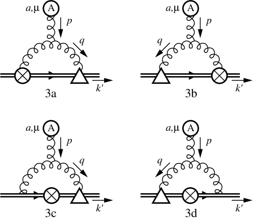
Figure 3: Diagrams involving $\displaystyle O_{kin}$ and $\displaystyle O_{mag}$ that renormalize $\displaystyle O_{2}$.

The diagram must, therefore, have two internal gluon lines. If $\displaystyle k^{\prime}$ or $\displaystyle q$ is to end up contracted with the $\displaystyle\sigma$ tensor, an internal gluon line has to contract with $\displaystyle O_{mag}$. There are only four such diagrams, shown in Figure 3. The calculation of the contribution of Figures 3a-b is described in more detail than the other parts of the calculation; it is a typical example of the process of calculating these divergences.

The amplitudes corresponding to these diagrams are

$$\displaystyle\int{d^{4}q\over(2\pi)^{4}} \displaystyle gf_{abc}[g_{\mu\kappa}(-2p_{\rho})+g_{\rho\kappa}(2q-p)_{\mu}+g_{\mu\rho}(2p_{\kappa})]$$ (15)

$$\displaystyle\times \displaystyle{-i\over(p-q)^{2}q^{2}(k^{\prime}-q)\cdot v}$$

$$\displaystyle\times \displaystyle\left(-g\over 2m\right)\sigma^{\kappa\alpha}q_{\alpha}T_{c}\left(ig\over 2m\right)(2k^{\prime}-q-p)^{\rho}T_{b}$$

from the diagram in Figure 3a, and

$$\displaystyle\int{d^{4}q\over(2\pi)^{4}} \displaystyle gf_{abc}[g_{\mu\kappa}(-2p_{\rho})-g_{\rho\kappa}(2q-p)_{\mu}+g_{\mu\rho}(2p_{\kappa})]$$ (16)

$$\displaystyle\times \displaystyle{-i\over(p-q)^{2}q^{2}(k^{\prime}-p+q)\cdot v}$$

$$\displaystyle\times \displaystyle\left(-g\over 2m\right)\sigma^{\rho\alpha}q_{\alpha}T_{c}\left(ig\over 2m\right)(2k^{\prime}-q-p)^{\kappa}T_{b}$$

from Figure 3b. The projection operator in the heavy quark propagator may be ignored, since all operators are assumed to be sandwiched between heavy quark fields, and in both cases the projector commutes with one of the vertex factors.

Taking only the terms with a single factor of $\displaystyle k^{\prime}$ contracted with $\displaystyle\sigma$, and adding the two diagrams together, gives

$$-2Ni{g^{3}\over(2m)^{2}}T_{a}k^{\prime}_{\beta}\sigma^{\beta\alpha}\int{d^{4}q\over(2\pi)^{4}}{q_{\alpha}(2q-p)_{\mu}\over(p-q)^{2}q^{2}}\left({1\over q\cdot v}+{1\over(q-p)\cdot v}\right)$$ (17)

where $\displaystyle N$ is the number of colors. The quadratic factors in the denominator may be combined using the usual method of Feynman parameters; shifting the integral to make it symmetric, and extracting only the term linear in $\displaystyle p$ yields

$$-2Ni{g^{3}\over(2m)^{2}}T_{a}k^{\prime}_{\beta}p_{\alpha}\sigma^{\beta\alpha}\int{d^{4}q\over(2\pi)^{4}}{q_{\mu}\over(q^{2})^{2}q\cdot v}$$ (18)

The heavy quark propagator factors remaining in the denominator may now be combined with the rest using the usual (for HQEFT) identity

$${1\over(q^{2})^{n}(q\cdot v)^{m}}={(n+m-1)!\over(n-1)!(m-1)!}\int^{\infty}_{0}{2^{m}\lambda^{m-1}d\lambda\over(q^{2}+2\lambda q\cdot v)^{n+m}}$$ (19)

where $\displaystyle\lambda$ is a sort of Feynman parameter with dimensions of mass. Then the integral over momentum space is

$$\int^{\infty}_{0}d\lambda\int{d^{4}q\over(2\pi)^{4}}4{q_{\mu}\over(q^{2}+2\lambda q\cdot v)^{3}}$$ (20)

Again shift the integral, $\displaystyle q\rightarrow q-\lambda v$,

$$\int^{\infty}_{0}d\lambda\int{d^{4}q\over(2\pi)^{4}}4{(q-\lambda v)_{\mu}\over(q^{2}-\lambda^{2})^{3}}$$ (21)

and remove the term that is odd in $\displaystyle q$; now the integral over $\displaystyle\lambda$ is easy, and the amplitude becomes

$$-2Ni{g^{3}\over(2m)^{2}}T_{a}k^{\prime}_{\beta}p_{\alpha}\sigma^{\beta\alpha}v_{\mu}\int{d^{4}q\over(2\pi)^{4}}{1\over(q^{2})^{2}}$$ (22)

Under $\displaystyle DR\overline{MS}$ in $\displaystyle 4-\epsilon$ dimensions, the amplitude is

$${4Ng^{2}\mu^{\epsilon}\over(4\pi)^{2}\epsilon}\cdot{g\over 4m^{2}}k^{\prime}_{\alpha}p_{\beta}\sigma^{\alpha\beta}v^{\mu}T_{a}.$$ (23)

In Figures 3c-d, contributions of the form of (13) arise from factors of the form $\displaystyle k^{\prime}\cdot qq_{\alpha}p_{\beta}\sigma^{\alpha\beta}$, via (14). Taken together, the relevant part of their contribution is

$${g^{3}\over 4m^{2}}4NiT_{a}v^{\mu}\sigma^{\gamma\alpha}p_{\gamma}k^{\prime\beta}\int{d^{4}q\over(2\pi)^{4}}{q_{\alpha}q_{\beta}\over(q^{2})^{2}(q\cdot v)^{2}}$$ (24)

After using Feynman parameters to combine the denominators and making the integrand symmetric, (14) may be used to obtain a term of the desired form, which is

$${-8Ng^{2}\mu^{\epsilon}\over(4\pi)^{2}\epsilon}\cdot{g\over 4m^{2}}k^{\prime}_{\alpha}p_{\beta}\sigma^{\alpha\beta}v^{\mu}T_{a}.$$ (25)

3.5 Diagrams with $\displaystyle O_{2}$

Some of the diagrams containing an insertion of $\displaystyle O_{2}$ may be eliminated in an analogous manner to the ones considered above. Here it is not necessary to take (14) into consideration, because an $\displaystyle O_{2}$ vertex and a three-gluon QCD vertex can together contribute at most three factors of momentum in the numerator.

The three-gluon $\displaystyle O_{2}$ vertex is completely nonderivative, so there is no way to obtain the desired factor of $\displaystyle k^{\prime}$ from that vertex.

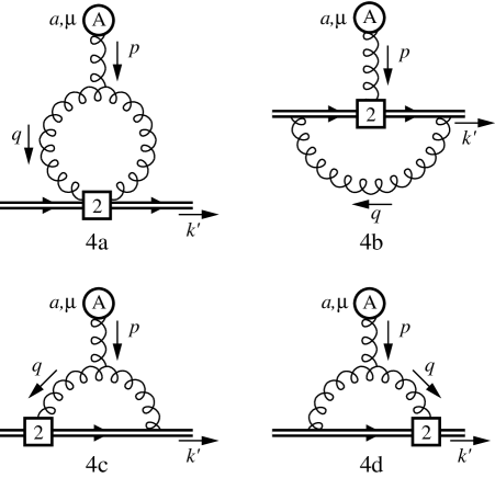
Figure 4: Diagrams involving $\displaystyle O_{2}$ that renormalize $\displaystyle O_{2}$.

The term in the two-gluon vertex that has the $\displaystyle k^{\prime}$ lacks any other factors of momentum, so the factor of $\displaystyle p$ must come from somewhere else. Therefore, any such diagram must have two internal gluon lines. The only possibility is Figure 4a.

With the one-gluon vertex, there will be no contribution from diagrams in which $\displaystyle O_{2}$ is connected to the sole internal gluon line, since then the gluon momentum in the vertex is $\displaystyle q$, and there are no other vertices with momenta in them. However, there is also the option of connecting $\displaystyle O_{2}$ directly to the external gluon leg, so that a factor of the desired form comes directly from the $\displaystyle O_{2}$ vertex. That is Figure 4b.

There are also diagrams with two internal gluon lines, one of which contracts with $\displaystyle O_{2}$’s one-gluon vertex; these are Figure 4c and Figure 4d.

The calculations proceed much as before. In each diagram, the terms to look for are the ones in which the momenta are appropriately contracted, keeping in mind that factors of a loop momentum $\displaystyle q$ can turn into factors of $\displaystyle p$ when the integration variable is shifted, if $\displaystyle p$ flows through an internal gluon line (but not if it only flows through an internal heavy quark line). The important term contributed by Figure 4a is

$${1\over 2}\cdot\int{d^{4}q\over(2\pi)^{4}}{g^{3}\over(2m)^{2}}NiT_{a}{1\over q^{2}(p-q)^{2}}(4k_{\alpha}p_{\rho}\sigma^{\alpha\rho}v_{\mu})$$ (26)

The $\displaystyle 1\over 2$ is the loop integral’s symmetry factor. Combining denominators in the usual way reveals that the $\displaystyle p$ in the denominator contributes only terms of higher than linear order in $\displaystyle p$ and may therefore be neglected (the story would have been different, had there been terms with factors of $\displaystyle q$ in the numerator). The divergent term linear in $\displaystyle p$ is

$$-{4Ng^{2}\mu^{\epsilon}\over(4\pi)^{2}\epsilon}\cdot{g\over 4m^{2}}k^{\prime}_{\alpha}p_{\beta}\sigma^{\alpha\beta}v^{\mu}T_{a}.$$ (27)

Figure 4b makes a small contribution, because of a group-theoretic factor of $\displaystyle-1\over 2N$; the term with the correct factors of $\displaystyle k$ and $\displaystyle p$ is

$${-ig^{3}\over(2m)^{2}}\left(-{1\over 2N}T_{a}\right)k^{\prime}_{\alpha}p_{\beta}\sigma^{\alpha\beta}v^{\mu}\int{d^{4}q\over(2\pi)^{4}}{1\over q^{2}(q\cdot v)^{2}},$$ (28)

which comes to

$$+{2g^{2}\mu^{\epsilon}\over N(4\pi)^{2}\epsilon}\cdot{g\over 4m^{2}}k^{\prime}_{\alpha}p_{\beta}\sigma^{\alpha\beta}v^{\mu}T_{a}.$$ (29)

Figures 4c and 4d contribute in much the manner of Figures 3a-b. The term of the desired form in Figure 4c, after combining the gluon denominators, shifting the loop variable, and doing the integral over the Feynman parameter, is

$$-{Ni\over 2}T_{a}{g^{3}\over 2m^{2}}k^{\prime}_{\alpha}p_{\beta}\sigma^{\alpha\beta}\int{d^{4}q\over(2\pi)^{4}}{2q\cdot vv_{\mu}-q_{\mu}\over(q^{2})^{2}q\cdot v}$$ (30)

Figure 4d’s contribution is identical. Adding the two together, combining with the heavy quark denominators and performing the requisite integrals gives

$$+{2Ng^{2}\mu^{\epsilon}\over(4\pi)^{2}\epsilon}\cdot{g\over 4m^{2}}k^{\prime}_{\alpha}p_{\beta}\sigma^{\alpha\beta}v^{\mu}T_{a}.$$ (31)

3.6 The $\displaystyle\beta$ function of $\displaystyle O_{2}$’s coefficient

These, then, are all of the divergent pieces of $\displaystyle\Gamma_{O_{2}}$, the part of the 1PI three-point function with the same form as (18). Adding them all together, including the coefficients from the Lagrangian, and putting in the contribution from the single vertex,

$$\displaystyle\Gamma_{O_{2}} \displaystyle= \displaystyle\left\{C_{2}+\left[-4NC_{kin}C_{mag}-\left(2N-{2\over N}\right)C_{2}\right]{g^{2}\over(4\pi)^{2}}\ln\mu\right\}$$ (32)

$$\displaystyle\times \displaystyle{g\over 4m^{2}}k^{\prime}_{\alpha}p_{\beta}\sigma^{\alpha\beta}v^{\mu}T_{a}+\cdots$$

where the dots represent convergent terms not dependent on $\displaystyle\mu$. Now the $\displaystyle\beta$ function for $\displaystyle C_{2}$ may be determined by solving the renormalization group equation for $\displaystyle\Gamma_{O_{2}}$:

$$\left(\mu{\partial\over\partial\mu}+\beta_{g}{\partial\over\partial g}+\beta_{mag}{\partial\over\partial C_{mag}}+\beta_{kin}{\partial\over\partial C_{kin}}+\beta_{2}{\partial\over\partial C_{2}}-2\gamma_{Q}-\gamma_{A}\right)\Gamma_{O_{2}}=0$$ (33)

$\displaystyle\beta_{kin}$ is zero ($\displaystyle C_{kin}$ does not run and is just equal to 1), the $\displaystyle\beta_{mag}$ term is higher order in $\displaystyle g$ than the others, and explicit gauge invariance in background field gauge means that the terms with $\displaystyle\beta_{g}$ and $\displaystyle\gamma_{A}$ cancel. The anomalous dimension of the heavy quark field is

$$\gamma_{Q}=-\left(N-{1\over N}\right){g^{2}\over(4\pi)^{2}}.$$ (34)

Solving for $\displaystyle\beta_{2}$ to order $\displaystyle g^{2}$,

$$\beta_{2}(g(\mu),C_{kin},C_{mag}(\mu))={g^{2}\over(4\pi)^{2}}\left(4NC_{kin}C_{mag}\right)$$ (35)

Remarkably, there is no multiplicative renormalization of $\displaystyle C_{2}$; the diagrams with $\displaystyle O_{2}$ insertions are completely canceled by the term from the heavy quark anomalous dimension. At the scale where matching occurs, $\displaystyle C_{mag}=C_{kin}=C_{2}=1$, and

$$\beta_{2}(g(m_{Q}),C_{kin},C_{mag}(m_{Q}))={4Ng^{2}\over(4\pi)^{2}}$$ (36)

Since every diagram except 4b contains a three-gluon QCD coupling, it is also interesting to consider the case of a $\displaystyle U(1)$ gauge theory, in which 4b is the only 1PI diagram that renormalizes $\displaystyle O_{2}$. Then 4b lacks the group-theoretic factor of $\displaystyle-1\over 2N$ that is present in the $\displaystyle SU(N)$ case, and the heavy quark anomalous dimension is $\displaystyle 2g^{2}\over(4\pi)^{2}$. The solution of the RGE to order $\displaystyle g^{2}$ is

$$\beta_{2}={g^{2}\over(4\pi)^{2}}(+4-4)C_{2}=0$$ (37)

so, for $\displaystyle U(1)$, $\displaystyle C_{2}$ does not run at all at one loop.

4 Renormalizing $\displaystyle O_{1}$ to one loop

4.1 Eliminating class II terms

The renormalization of $\displaystyle O_{1}$ is slightly more involved, conceptually and mathematically, for two reasons. First, there are more diagrams to consider; second, the simplest vertex of $\displaystyle O_{1}$ has no term that cannot be produced by class II operators as well, so it is necessary to calculate the part of each diagram that renormalizes one of the class II operators, and subtract it out. Fortunately, these two difficulties cancel each other out to some extent, because many of the extra diagrams turn out to renormalize only the class II operator.

The term in the one-gluon vertex of $\displaystyle O_{1}$ that gives the least trouble is

$${ig\over 8m^{2}}(p^{2}v^{\mu})T_{a}.$$ (38)

This term also appears in the one-gluon vertex of the class II operator $\displaystyle{1\over 8m^{2}}\overline{\psi}_{+v}\{iD\cdot v,D^{2}\}\psi_{+v}$. However, in this operator the factor $\displaystyle p^{2}v^{\mu}$ always shows up in the combination $\displaystyle(-2k^{\prime}\cdot p+p^{2})v^{\mu}$, and the $\displaystyle k^{\prime}\cdot pv^{\mu}$ term is not produced by any other local operator to order $\displaystyle 1\over m^{2}$. Therefore, to subtract out the renormalization of the class II operator, all that is necessary is to add, in the divergent term of each diagram, half the coefficient of

$${ig\over 8m^{2}}(k^{\prime}\cdot pv^{\mu})T_{a}$$ (39)

to the coefficient of (38).

Both of these terms are spin-independent. Therefore, contributions to the renormalization may come from double insertions of $\displaystyle O_{kin}$, from double insertions of $\displaystyle O_{mag}$, or from single insertions of $\displaystyle O_{1}$ itself.

4.2 Diagrams with one internal gluon line

The expression (38) has no factor of $\displaystyle k^{\prime}$ in it, so it is now possible to obtain nonzero contributions to the running of $\displaystyle O_{1}$ from diagrams in which no factors of $\displaystyle k^{\prime}$ appear in the vertices. There may be a contribution if the numerator, prior to loop integration, contains factors like $\displaystyle k^{\prime}\cdot p$, $\displaystyle p^{2}$, $\displaystyle k^{\prime}\cdot qp\cdot q$, or $\displaystyle p\cdot qp\cdot q$. If there is only one internal gluon line, these factors cannot arise from the propagators, for precisely the same reasons as in the $\displaystyle O_{2}$ case. Routing the loop momentum $\displaystyle q$ through the lone gluon line reveals that its denominator is simply $\displaystyle q^{2}$, and factors of $\displaystyle k^{\prime}$, $\displaystyle p$, or $\displaystyle q$ in the quark denominators are contracted with $\displaystyle v$.

Therefore, in such diagrams, the factors of $\displaystyle k^{\prime}$ and $\displaystyle p$ in the divergence must appear explicitly in the vertex factors prior to loop integration, and the external momenta must be contracted with each other or with $\displaystyle q^{\mu}q^{\nu}$.

Class II contributions may also be neglected. If the factors of the form of $\displaystyle p^{2}$ and $\displaystyle k^{\prime}\cdot p$ appear in the combination $\displaystyle p^{2}-2k^{\prime}\cdot p$, then the divergence just renormalizes a class II operator, and it need not be considered.

4.3 Diagrams with two internal gluon lines

When there are two internal gluon lines, additional complications arise. Factors of $\displaystyle p^{2}$ can and do arise in the gluon propagators. Therefore, when calculating the divergent term of the form of (38), it is necessary to expand the loop integrand in powers of $\displaystyle p^{2}$ and retain the zeroth- and first-order terms. For this reason, the calculation of these diagrams is more involved than for $\displaystyle O_{1}$.

4.4 Diagrams with $\displaystyle O_{kin}$

Terms like (38) and (39) arise from many diagrams with two $\displaystyle O_{kin}$ vertices.

4.4.1 The gluonless vertex

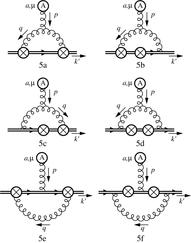
Figure 5: Diagrams involving $\displaystyle O_{kin}$ that renormalize $\displaystyle O_{1}$.

In particular, it seems as if contributions to both ought to come from any diagram with a no-gluon vertex on a quark line carrying some linear combination of $\displaystyle k^{\prime}$ and $\displaystyle p$ (and possibly the loop momentum $\displaystyle q$). This is indeed the case for the diagrams with two internal gluon lines (as in Figures 5b-d).

If there is only one internal gluon line, the possibilities are more restricted. If there is also only one gluonless vertex, then there can be at most three factors of momentum and (14) cannot provide the desired contractions. Routing $\displaystyle q$ through the gluon line implies that the quark line on which the $\displaystyle O_{kin}$ vertex sits may only carry either $\displaystyle k^{\prime}\pm q$ or $\displaystyle k^{\prime}-p\pm q$. In the former case, the gluonless $\displaystyle O_{kin}$ vertex provides neither a term like (38) nor one like (39). In the latter case, the terms appear in the class II combination and may be ignored.

If there is one internal gluon line but two gluonless $\displaystyle O_{kin}$ vertices, it becomes possible to obtain contributions via (14). If both of them are on the same side of the external gluon leg, however, the momentum factors are of the same form as those of a single vertex, and the diagrams may be excluded by the arguments in the previous paragraph. The only class I contribution occurs when the gluonless vertices are on opposite sides of the external gluon leg, as in Figure 5f.

4.4.2 The one-gluon vertex

The one-gluon vertex has uncontracted momenta in it; factors of $\displaystyle k^{\prime}\cdot p$ and $\displaystyle p^{2}$ may be produced by putting it in a diagram with two internal gluon lines (Figures 5a-c) or by contracting it with another one-gluon $\displaystyle O_{kin}$ vertex (Figure 5e).

4.4.3 Eliminating the two-gluon vertex

The two-gluon vertex is completely nonderivative, so any diagram with that one in it would have to get its factors of $\displaystyle k^{\prime}\cdot p$ or $\displaystyle p^{2}$ from somewhere else. If there is only one internal gluon line, then, as stated above, these factors would have to come from the other $\displaystyle O_{kin}$ vertex. They can’t, since they could only arise from the no-gluon vertex, and that only supplies them in a class II combination if there is only one internal gluon line. Therefore, the two-gluon $\displaystyle O_{kin}$ vertex can only contribute if there are two internal gluon lines.

But if the diagram is to be 1PI, then one of those has to connect to something other than the two-gluon $\displaystyle O_{kin}$ vertex, which leaves it with an extra leg. So this vertex doesn’t contribute at all.

The diagrams in Figure 5 are therefore all of the contributions to the renormalization of $\displaystyle O_{1}$ from double insertions of $\displaystyle O_{kin}$. When calculating them, it is necessary to do the expansions in $\displaystyle p^{2}$ mentioned above.

For example, consider Figure 5a. After the usual manipulations to combine the gluon denominators, shift the integrand, and throw out terms proportional to $\displaystyle k^{\prime 2}$ or $\displaystyle k^{\prime}\cdot v$ or to four-vectors other than $\displaystyle v^{\mu}$ or $\displaystyle q^{\mu}$, the leftover amplitude looks like

$$\displaystyle- \displaystyle{g^{3}\over(2m)^{2}}{NT_{a}\over 2}\int^{1}_{0}dx\int{d^{4}q\over(2\pi)^{4}}{1\over[q^{2}+x(1-x)p^{2}]^{2}(q\cdot v)}2q^{\mu}$$ (40)

$$\displaystyle\times \displaystyle[(x^{2}+x+1)p^{2}+q^{2}+(1+2x)p\cdot q-4k^{\prime}\cdot q-2(1+2x)k^{\prime}\cdot p]$$

Expanding the factor with the denominators

$${1\over[q^{2}+x(1-x)p^{2}]^{2}}\rightarrow{1\over(q^{2})^{2}}-{2x(1-x)p^{2}\over(q^{2})^{3}}+\cdots$$ (41)

reveals the presence of additional $\displaystyle p^{2}$ terms in the result. The relevant divergent terms turn out to be

$${g^{3}\over(2m)^{2}}T_{a}\left(4Nk^{\prime}\cdot p+{N\over 2}p^{2}\right)v^{\mu}\int{d^{4}q\over(2\pi)^{4}}{1\over(q^{2})^{2}}$$ (42)

Subtracting out the class II contribution, by adding the coefficient of the $\displaystyle p^{2}$ term to half the coefficient of the $\displaystyle k^{\prime}\cdot p$ term, makes this

$${10Ng^{2}\mu^{\epsilon}\over(4\pi)^{2}\epsilon}{ig\over 8m^{2}}T_{a}p^{2}v^{\mu}+(II)$$ (43)

where (II) refers to the part that renormalizes an operator that vanishes by the equation of motion.

Figures 5b and 5c together contribute

$$-2N{g^{3}\over(2m)^{2}}T_{a}(k^{\prime}\cdot p-p^{2})v^{\mu}\int{d^{4}q\over(2\pi)^{4}}{1\over(q^{2})^{2}}$$ (44)

which is

$${4Ng^{2}\mu^{\epsilon}\over(4\pi)^{2}\epsilon}{ig\over 8m^{2}}T_{a}p^{2}v^{\mu}+(II),$$ (45)

and Figure 5d contributes

$${g^{3}\over(2m)^{2}}T_{a}(-8Nk^{\prime}\cdot p+2Np^{2})v^{\mu}\int{d^{4}q\over(2\pi)^{4}}{1\over(q^{2})^{2}}$$ (46)

which is

$${-8Ng^{2}\mu^{\epsilon}\over(4\pi)^{2}\epsilon}{ig\over 8m^{2}}T_{a}p^{2}v^{\mu}+(II).$$ (47)

Figures 5e-f have a different group-theoretic structure; 5e’s contribution is

$$-{16\over N}{g^{2}\mu^{\epsilon}\over(4\pi)^{2}\epsilon}{ig\over 8m^{2}}T_{a}k\cdot pv^{\mu}$$ (48)

which is

$$-{8\over N}{g^{2}\mu^{\epsilon}\over(4\pi)^{2}\epsilon}{ig\over 8m^{2}}T_{a}p^{2}v^{\mu}+(II).$$ (49)

and fig:kinkinonef’s is

$$\left(-{1\over 2N}T_{a}\right){g^{3}\over 4m^{2}}v^{\mu}\int{d^{4}q\over(2\pi)^{4}}{q^{2}(p^{2}-2k^{\prime}\cdot p)-4k^{\prime}\cdot qp\cdot q\over q^{2}(q\cdot v)^{4}}$$ (50)

which, after combining denominators, shifting the integration variable, and applying (14), becomes

$${8\over 3N}{g^{2}\mu^{\epsilon}\over(4\pi)^{2}\epsilon}{ig\over 8m^{2}}T_{a}p^{2}v^{\mu}+(II).$$ (51)

In this case the entire class I contribution comes from (14).

4.5 Diagrams with $\displaystyle O_{mag}$

Double insertions of $\displaystyle O_{mag}$ will produce no factors of $\displaystyle k^{\prime}\cdot p$, since in such diagrams the only factors of $\displaystyle k^{\prime}$ are in heavy quark propagators. Therefore, it is only necessary to seek out factors of $\displaystyle p^{2}v^{\mu}$.

If the diagram has only one internal gluon line, at least one of the $\displaystyle O_{mag}$ vertices will be connected to it, so its vertex will contain a factor of $\displaystyle q$ rather than $\displaystyle p$. Then there is no way of obtaining two factors of $\displaystyle p$ explicitly in the quark-gluon vertex factors; (14) does not apply, since there is no way to obtain four factors of momentum in the numerator.

There must be two internal gluon lines. That leaves only Figure 6.

In this calculation, the projector in the heavy quark propagator must not be neglected, since it does not commute with $\displaystyle\sigma^{\mu\nu}$ [7]. When extracting the spin-independent part of this diagram’s amplitude, one may use the identities

$$\sigma^{\alpha\mu}\left({1+\hbox to0.0pt{$\displaystyle v$\hss}/\over 2}\right)\sigma_{\alpha\nu}=2\delta^{\mu}_{\nu}-2v^{\mu}v_{\nu}+\hbox{spin-dependent terms}$$ (52)

and

$$\displaystyle\sigma_{\mu\alpha}\left({1+\hbox to0.0pt{$\displaystyle v$\hss}/\over 2}\right)\sigma_{\beta\nu}p^{\alpha}p^{\beta} \displaystyle= \displaystyle-g_{\mu\nu}p^{2}+g_{\mu\nu}(p\cdot v)^{2}+p_{\mu}p_{\nu}+p^{2}v_{\mu}v_{\nu}$$ (53)

$$\displaystyle-v_{\mu}p_{\nu}p\cdot v-p_{\mu}v_{\nu}p\cdot v+\hbox{spin-dependent terms}$$

where both expressions are assumed to be sandwiched between heavy-quark spinors, so that factors of $\displaystyle\hbox to0.0pt{$\displaystyle v$\hss}/$ may be dropped at the beginning or end of a term.

Figure 6’s contribution is

$${10Ng^{2}\mu^{\epsilon}\over 3(4\pi)^{2}\epsilon}{ig\over 8m^{2}}T_{a}p^{2}v^{\mu}.$$ (54)

There is no class II term.

4.6 Diagrams with $\displaystyle O_{1}$

In the multiplicative renormalization from insertions of $\displaystyle O_{1}$, no $\displaystyle k^{\prime}\cdot pv^{\mu}$ terms arise, so there are no class II renormalizations to subtract away. Again, (14) does not apply since there are at most three factors of momentum in the numerator.

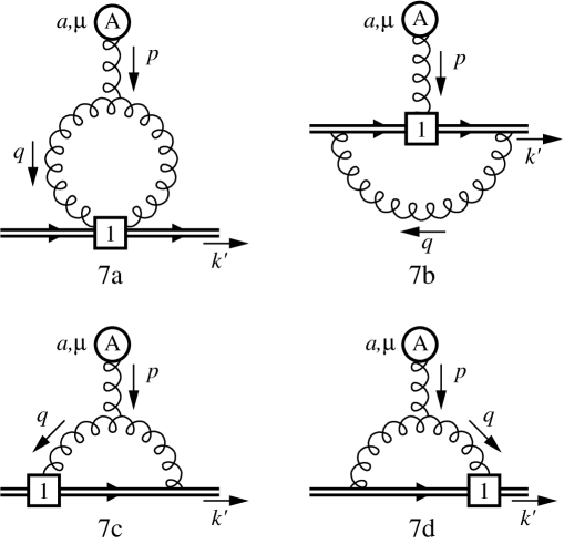
Figure 7: Diagrams involving $\displaystyle O_{1}$ that renormalize $\displaystyle O_{1}$.

If there is only one internal gluon line and it contracts with any of the $\displaystyle O_{1}$ vertices, a factor of $\displaystyle p^{2}$ cannot arise explicitly in the vertex factors, since the only vertex with two factors of momentum in it is the one-gluon vertex, and in that case the momentum will be $\displaystyle q$. The only diagram left that has one internal gluon line is Figure 7b.

The other possibilities have two internal gluon lines, one of which contracts with an $\displaystyle O_{1}$ vertex. These are Figures 7a, 7c, and 7d. When calculating these diagrams, it is necessary to expand combined gluon denominators as series in $\displaystyle p^{2}$, as before.

Figure 7a’s symmetry factor is $\displaystyle 1\over 2$, as for Figure 4a. The relevant divergent term is

$$-{5Ng^{2}\mu^{\epsilon}\over(4\pi)^{2}\epsilon}{ig\over 8m^{2}}T_{a}p^{2}v^{\mu}.$$ (55)

Figure 7b gives

$$+{2g^{2}\mu^{\epsilon}\over N(4\pi)^{2}\epsilon}{ig\over 8m^{2}}T_{a}p^{2}v^{\mu}$$ (56)

much in the manner of Figure 4b’s contribution to the renormalization of $\displaystyle O_{2}$. Finally, Figures 7c and 7d together give

$${g^{3}\over 8m^{2}}T_{a}{5N\over 6}p^{2}v^{\mu}\int{d^{4}q\over(2\pi)^{4}}$$ (57)

or

$${5Ng^{2}\mu^{\epsilon}\over 3(4\pi)^{2}\epsilon}{ig\over 8m^{2}}T_{a}p^{2}v^{\mu}.$$ (58)

4.7 The $\displaystyle\beta$ function of $\displaystyle O_{1}$’s coefficient

The calculation of $\displaystyle\beta_{1}$ is analogous to that of $\displaystyle\beta_{2}$. The three-point 1PI function of the form of (38), with class II divergences subtracted, is

$$\displaystyle\Gamma_{O_{1}} \displaystyle= \displaystyle\left\{C_{1}+\left[\left(6N-{16\over 3N}\right)C_{kin}^{2}+{10N\over 3}C_{mag}^{2}+\left(-{10N\over 3}+{2\over N}\right)C_{1}\right]{g^{2}\over(4\pi)^{2}}\ln\mu\right\}$$ (59)

$$\displaystyle\times \displaystyle{g\over 8m^{2}}p^{2}v^{\mu}T_{a}+\cdots$$

where the dots represent convergent terms not dependent on $\displaystyle\mu$. Solving the RGE

$$\left(\mu{\partial\over\partial\mu}+\beta_{g}{\partial\over\partial g}+\beta_{kin}{\partial\over\partial C_{kin}}+\beta_{mag}{\partial\over\partial C_{mag}}+\beta_{1}{\partial\over\partial C_{1}}-2\gamma_{Q}-\gamma_{A}\right)\Gamma_{O_{1}}=0$$ (60)

to order $\displaystyle g^{2}$ gives

$$\beta_{1}(g(\mu),C_{kin},C_{1}(\mu))={g^{2}\over(4\pi)^{2}}\left[\left(-6N+{16\over 3N}\right)C_{kin}^{2}-{10N\over 3}C_{mag}^{2}+{4N\over 3}C_{1}\right].$$ (61)

$\displaystyle C_{kin}=1$. At the scale where matching occurs, $\displaystyle C_{1}=C_{mag}=1$, and

$$\beta_{1}(g(m_{Q}),C_{kin},C_{1}(m_{Q}))=\left(-8N+{16\over 3N}\right){g^{2}\over(4\pi)^{2}}.$$ (62)

Figures 5e-f and 7b are the only diagrams present in an abelian gauge theory. 7b contributes to the renormalization of $\displaystyle O_{1}$ in exactly the same way that Figure 4b renormalizes $\displaystyle O_{2}$. 5e-f’s contribution is as above only without the $\displaystyle SU(N)$ factor of $\displaystyle-1\over 2N$. Therefore, at one loop in a $\displaystyle U(1)$ theory,

$$\displaystyle\beta_{1} \displaystyle= \displaystyle{g^{2}\over(4\pi)^{2}}\left[-{32\over 3}C_{kin}^{2}+(4-4)C_{1}\right]$$ (63)

$$\displaystyle= \displaystyle-{32\over 3}C_{kin}^{2}{g^{2}\over(4\pi)^{2}}$$

Other than the gauge coupling constant and the field normalizations, this is the only thing that runs at one loop to order $\displaystyle 1\over m^{2}$ in a $\displaystyle U(1)$ theory.

5 Reparameterization invariance is satisfied

In HQEFT, the division of the quark momentum into a large part $\displaystyle mv^{\mu}$ and a small residual momentum $\displaystyle k^{\mu}$ is arbitrary, as long as the residual momentum remains small. Therefore, there exists a symmetry of HQEFT called reparameterization invariance, in which the four-velocity and residual momentum change so as to leave the combination $\displaystyle mv^{\mu}+k^{\mu}$ invariant.[10] This places constraints on the coefficients of the correction terms.

However, it is first necessary to define how the heavy quark field transforms under a reparameterization. There are at least two different forms of reparameterization invariance in the literature, that of Luke and Manohar [10] and that of Chen [11]. Straightforward calculations show that the Lagrangian obtained from tree-level matching (before the field redefinition that removes the class II operators) is invariant under Chen’s transformation, but not under Luke and Manohar’s. Chen’s transformation

$$\displaystyle v^{\mu} \displaystyle\rightarrow \displaystyle v^{\mu}+\delta v^{\mu}$$

$$\displaystyle\psi_{+v} \displaystyle\rightarrow \displaystyle\left[1+{\delta\hbox to0.0pt{$\displaystyle v$\hss}/\over 2}\left(1+{1\over 2m+i{D\cdot v}}\right)\right]\psi_{+v}$$ (64)

does the following to the Lagrangian $\displaystyle{\cal L}=\overline{\psi}_{+v}A\psi_{+v}$ to order $\displaystyle 1\over m$:

$$\delta{\cal L}=\overline{\psi}_{+v}\left(\delta A+[A,im\delta vx]+\left\{A,{\delta\hbox to0.0pt{$\displaystyle v$\hss}/\over 2}\right\}+{i{{\hbox to0.0pt{$\displaystyle D$\hss}\thinspace/\thinspace}}_{\perp}\over 4m}\delta\hbox to0.0pt{$\displaystyle v$\hss}/A+A\delta\hbox to0.0pt{$\displaystyle v$\hss}/{i{{\hbox to0.0pt{$\displaystyle D$\hss}\thinspace/\thinspace}}_{\perp}\over 4m}\right)\psi_{+v}+O\left(1\over m^{2}\right)$$ (65)

where $\displaystyle{\hbox to0.0pt{$\displaystyle D$\hss}\thinspace/\thinspace}_{\perp}={\hbox to0.0pt{$\displaystyle D$\hss}\thinspace/\thinspace}-D\cdot v\hbox to0.0pt{$\displaystyle v$\hss}/$. (Because of the term proportional to $\displaystyle m$, we would need to know about $\displaystyle 1\over m^{3}$ terms in the Lagrangian to evaluate what the transformation does to order $\displaystyle 1\over m^{2}$.)

Applying (65) to (11) induces a change in the Lagrangian

$$\displaystyle\delta{\cal L} \displaystyle= \displaystyle\overline{\psi}_{+v}(1-C_{kin})iD\cdot\delta v\psi_{+v}+{1\over 4m}\overline{\psi}_{+v}\left[-D\cdot\delta v{D\cdot v}-{D\cdot v}D\cdot\delta v\right.$$ (66)

$$\displaystyle+\left.(1-2C_{mag}+C_{2})(iD^{\mu}\delta v^{\nu}\sigma_{\mu\nu}{D\cdot v}-i{D\cdot v}D^{\mu}\delta v^{\nu}\sigma_{\mu\nu})\right]\psi_{+v}.$$

The field-redefinition procedure we have used is equivalent in its effect on the running of the class I operators to throwing out all class II terms. Insertions of the class II terms does not affect the running of the class I terms, because the class I parts of the loop diagrams involving class II operators are finite. The poles that arise from solutions of the classical equation of motion are eliminated by the vanishing of the class II vertices. Therefore, our procedure will yield the same running for the class I operators that we would get if we kept all of the operators, class I and class II.

The tree-level Lagrangian, including the class II operators, is symmetric under the RPI symmetry in (65). Therefore, even using our procedure, as long as the regularization procedure preserves the RPI symmetry in (65), the renormalized Lagrangian to order $\displaystyle 1\over m^{2}$ must be symmetric under this transformation, up to terms resulting from the action of the transformation on the removed class II operators. The $\displaystyle-D\cdot\delta v{D\cdot v}-{D\cdot v}D\cdot\delta v$ term in (66) results from the action of the transformation on $\displaystyle O_{D\cdot v}$, so there is no reason to expect that term to vanish. The others, however, cannot be so obtained. Therefore, reparameterization invariance sets the constraints

$$\displaystyle C_{kin} \displaystyle= \displaystyle 1$$

$$\displaystyle 2C_{mag} \displaystyle= \displaystyle C_{2}+1$$ (67)

At matching, all of these constants are equal to 1, and the constraints are satisfied. Under running, in order to maintain these relations, it must be that

$$\displaystyle\beta_{kin} \displaystyle= \displaystyle 0$$

$$\displaystyle 2\beta_{mag} \displaystyle= \displaystyle\beta_{2}$$ (68)

It is well known that the first relation holds to the orders that have been studied. The second also holds at one loop, according to our results. The running satisfies reparameterization invariance in the form described by Chen.

6 Comparison with other recent calculations

In this section, we compare to results in [4, 5]

While this work was in preparation, a paper by Balzereit and Ohl was posted on the net [4], which also calculates the renormalization of the $\displaystyle 1/m^{2}$ operator, Their technique is quite different from ours; most importantly, they retain all class II operators, including $\displaystyle O_{D\cdot v}$. However, insertions of class II operators do not induce any class I counterterms, since the amplitudes resulting from class II insertions are finite. The poles that arise from solutions of the classical equations of motion are eliminated by the vanishing of the class II vertices. Therefore, a calculation using our technique, which assumes that the Lagrangian contains only class I operators, will yield the same $\displaystyle\beta$ functions (or, equivalently, anomalous dimensions of local operators and time-ordered products) obtained in [4] for the class I operators.

Balzereit and Ohl use a slightly different operator basis, but their basis for the class I operators is the same as ours up to class II terms and a sign difference in $\displaystyle O_{1}$.

Even given the class II terms by which our basis for the order $\displaystyle 1\over m^{2}$ local class I operators differs from [4], the results still have to be equivalent. With both operator bases, our technique can be used and the calculation will differ in no essential respect. For example, to renormalize $\displaystyle O_{1}$ in the basis of [4], one could look for terms of the form $\displaystyle 2k^{\prime}\cdot pv^{\mu}$, and subtract out class II terms of the form $\displaystyle(2k^{\prime}\cdot p-p^{2})v^{\mu}$ by adding twice the coefficient of $\displaystyle 2p^{2}v^{\mu}$ to the coefficient of $\displaystyle 2k^{\prime}\cdot pv^{\mu}$. This is manifestly the same calculation, and so the results must be the same, because the class II terms by which our operator bases differ do not affect the calculated coefficients of the $\displaystyle p^{2}v^{\mu}$ and $\displaystyle k^{\prime}\cdot pv^{\mu}$ terms.

Indeed, our results are equivalent to those of [4]. They define $\displaystyle O_{1}$ with the opposite sign, which reverses the signs of the contributions to $\displaystyle O_{1}$ from double $\displaystyle O_{kin}$ and double $\displaystyle O_{mag}$ insertions. Our definitions of $\displaystyle\beta$ functions also differ from their definitions of anomalous dimensions by a further factor of $\displaystyle-4{g^{2}/(4\pi)^{2}}$. Taking these into account, the terms in our $\displaystyle\beta$ functions are equivalent to the various elements in their anomalous dimension matrix $\displaystyle{\hat{\gamma}}^{(2)}_{phys}$. The nonzero anomalous dimensions in the first column correspond to the coefficients of $\displaystyle C_{1}$, $\displaystyle C_{kin}^{2}$, and $\displaystyle C_{mag}^{2}$ in our expression for $\displaystyle\beta_{1}$. The nonzero anomalous dimension in the second column corresponds to the coefficient of $\displaystyle C_{kin}C_{mag}$ in our $\displaystyle\beta_{2}$.

Very shortly before we posted this paper to the net, another calculation of the renormalization of the order $\displaystyle 1/m^{2}$ operators by B. Blok et al. [5] appeared. This calculation, like that of Balzereit and Ohl, retaines all class II operators, and expresses results in the form of anomalous dimensions mixing local operators with time-ordered products. The class I operator basis in [5] is the same as ours up to total derivatives, except for a sign difference in the definition of $\displaystyle O_{mag}$. The results for the class I operators also agree with ours, when this sign difference is taken into account; the first two columns of the matrix (22a) in [5] agree with the terms in our beta functions for the case $\displaystyle N=3$.

7 Conclusions

We have calculated the running of the heavy quark effective field theory Lagrangian to order $\displaystyle 1\over m^{2}$, using a technique in which continuous field redefinition removes operators from the Lagrangian which vanish according to the classical equation of motion. Our results are consistent with symmetry under the reparameterization transformation of [11]. Our results are inconsistent with those of [2] and agree with those of [4, 5].

Appendix A HQEFT Feynman rules to order $\displaystyle 1\over m^{2}$

The operators of HQEFT induce various Feynman vertices. In addition to the rules listed below, there are of course the usual QCD rules for gluons; we use background field gauge with a Feynman-like gauge prescription (at one loop, the gauge fixing parameter does not run and Feynman-like gauge is OK), so the gluon rules are as given in Abbott [6] with $\displaystyle\alpha=1$. The covariant derivative and gluon field-strength tensor are defined as follows:

$$D^{\mu}=\partial^{\mu}-igT_{a}A^{\mu}_{a}$$ (69)

$$G^{\mu\nu}={i\over g}[D^{\mu},D^{\nu}]=\partial^{\mu}A_{a}^{\nu}T_{a}-\partial^{\nu}A_{a}^{\mu}T_{a}+gf_{abc}T_{a}A_{b}^{\mu}A_{c}^{\nu}$$ (70)

It is convenient to express the rules in terms of the outgoing heavy quark’s residual momentum $\displaystyle k^{\prime\mu}$ (taken as flowing out of the vertex) and the gluon momenta $\displaystyle p^{\mu}$, $\displaystyle q^{\mu}$, and $\displaystyle r^{\mu}$ (which flow into the vertex). $\displaystyle a$, $\displaystyle b$, and $\displaystyle c$ are external gluon color indices. The vertices from the subleading operators are pictured in Figures 1 and 2.

A.1 Leading-order Lagrangian

A.1.1 propagator

$${i\over k^{\prime}\cdot v}\left({1+\hbox to0.0pt{$\displaystyle v$\hss}/\over 2}\right)$$ (71)

A.1.2 one-gluon vertex

$$igT_{a}v^{\mu}$$ (72)

A.2 $\displaystyle O_{kin}$

A.2.1 no-gluon vertex

$${i\over 2m}k^{\prime 2}$$ (73)

A.2.2 one-gluon vertex

$${ig\over 2m}(2k^{\prime}-p)^{\mu}T_{a}$$ (74)

A.2.3 two-gluon vertex

$${ig^{2}\over 2m}\left\{T_{a},T_{b}\right\}g^{\mu\nu}$$ (75)

A.3 $\displaystyle O_{mag}$

A.3.1 one-gluon vertex

$${-g\over 2m}\sigma^{\mu\nu}(p_{\nu}T_{a})$$ (76)

A.3.2 two-gluon vertex

$${ig^{2}\over 2m}\sigma^{\mu\nu}f_{abd}T_{d}$$ (77)

A.4 $\displaystyle O_{1}$

A.4.1 one-gluon vertex

$${-ig\over 8m^{2}}(p^{\mu}p\cdot v-p^{2}v^{\mu})T_{a}$$ (78)

A.4.2 two-gluon vertex

$${g^{2}\over 8m^{2}}[(q-p)\cdot vg^{\mu\nu}-(p+2q)^{\mu}v^{\nu}+(2p+q)^{\nu}v^{\mu}]f_{abd}T_{d}$$ (79)

A.4.3 three-gluon vertex

$$\displaystyle{-ig^{3}\over 8m^{2}}[(g^{\mu\rho}v^{\nu}-g^{\nu\mu}v^{\rho})f_{bcd}f_{dae}T_{e} \displaystyle+ \displaystyle(g^{\nu\mu}v^{\rho}-g^{\rho\nu}v^{\mu})f_{cad}f_{dbe}T_{e}$$ (80)

$$\displaystyle+ \displaystyle(g^{\rho\nu}v^{\mu}-g^{\mu\rho}v^{\nu})f_{abd}f_{dce}T_{e}]$$

A.5 $\displaystyle O_{2}$

A.5.1 one-gluon vertex

$${g\over 8m^{2}}(2k^{\prime}_{\alpha}p_{\beta}\sigma^{\alpha\beta}v^{\mu}-p\cdot v(2k^{\prime}-p)_{\alpha}\sigma^{\alpha\mu})T_{a}$$ (81)

A.5.2 two-gluon vertex

$$\displaystyle{g^{2}\over 8m^{2}}[(2k^{\prime}_{\alpha}-p_{\alpha}-q_{\alpha})if_{abc}T_{c}(\sigma^{\alpha\mu}v^{\nu}-\sigma^{\alpha\nu}v^{\mu})$$

$$\displaystyle+(-p_{\alpha}\sigma^{\alpha\nu}v^{\mu}-q_{\alpha}\sigma^{\alpha\mu}v^{\nu} \displaystyle+ \displaystyle(p-q)\cdot v\sigma^{\mu\nu})\{T^{a},T^{b}\}]$$ (82)

A.5.3 three-gluon vertex

$$\displaystyle{-ig^{3}\over 8m^{2}}[(\sigma^{\mu\rho}v^{\nu}+\sigma^{\nu\mu}v^{\rho})f_{bcd}\{T_{a},T_{d}\} \displaystyle+ \displaystyle(\sigma^{\nu\mu}v^{\rho}+\sigma^{\rho\nu}v^{\mu})f_{cad}\{T_{b},T_{d}\}$$ (83)

$$\displaystyle+ \displaystyle(\sigma^{\rho\nu}v^{\mu}+\sigma^{\mu\rho}v^{\nu})f_{abd}\{T_{c},T_{d}\}]$$

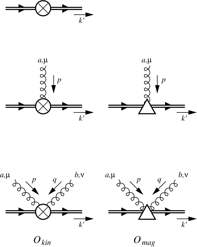
Figure 1: Feynman vertices induced by the operators $\displaystyle O_{kin}$ and $\displaystyle O_{mag}$.

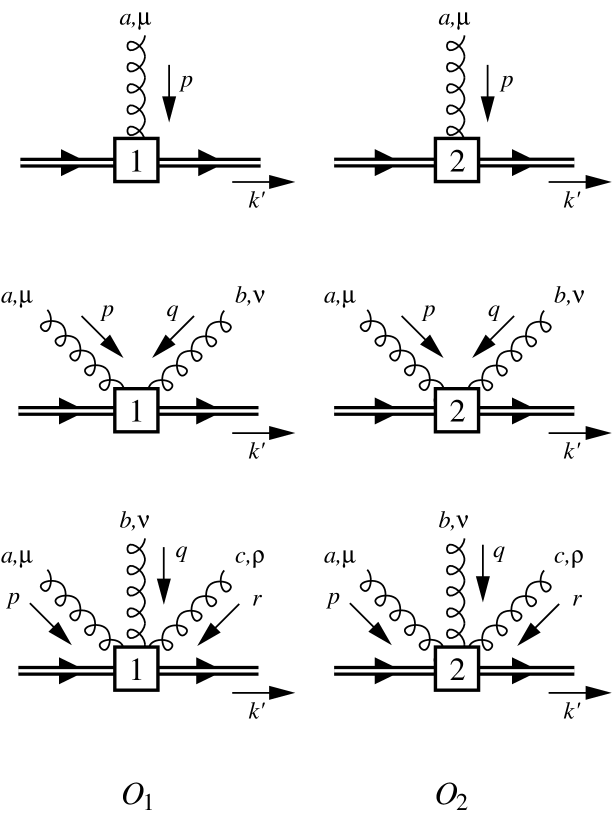
Figure 2: Feynman vertices induced by the operators $\displaystyle O_{1}$ and $\displaystyle O_{2}$.

Figure 6: Diagram involving $\displaystyle O_{mag}$ that renormalizes $\displaystyle O_{1}$.

References

- [1] M. Neubert, Phys. Reports 245 (1994) 259.
- [2] C. L. Y. Lee, CALT-68-1663 (1991).
- [3] S. Balk, J.G. Körner, D. Pirjol, Nucl. Phys. B 428 (1994) 499;
- [4] C. Balzereit and T. Ohl, IKDA 96/11, hep-ph/9604352 (1996).
- [5] B. Blok, J.G. Körner, D. Pirjol, J.C. Rojas, hep-ph/9607233
- [6] L. F. Abbott, Nuc. Phys. B185 (1981), 189.
- [7] We thank C. Balzereit and T. Ohl for pointing this out to us.
- [8] A. F. Falk, B. Grinstein, and M. E. Luke, Nuc. Phys. B357 (1991), 185.
- [9] W. Kilian and T. Mannel, Phys. Rev. D49 (1994), 1534.
- [10] M. E. Luke and A. V. Manohar, Phys. Lett. B286 (1992) 348.
- [11] Y.-Q. Chen, Phys. Lett. B317 (1993), 421.