IP-ASTP-03-96
Status of the Proton Spin Problem^∗

Abstract

The proton spin problem triggered by the EMC experiment and its present status are closely examined. Recent experimental and theoretical progresses and their implications are reviewed. It is pointed out that the sign of the sea-quark polarization generated perturbatively by hard gluons via the anomaly mechanism is predictable: It is negative if the gluon spin component is positive. We stress that the polarized nucleon structure function $g_{1}(x)$ is independent of the $k_{\perp}$-factorization scheme chosen in defining the quark spin density and the hard photon-gluon scattering cross section. Consequently, the anomalous gluon and sea-quark interpretations for $\Gamma_{1}$, the first moment of $g_{1}(x)$, are equivalent. It is the axial anomaly that accounts for the observed suppression of $\Gamma_{1}^{p}$.

^∗ Lecture presented at the

Xth Spring School on Particles and Fields

National Cheng-Kung University, Taiwan, ROC

March 20-22, 1996

1 Introduction

Experiments on polarized deep inelastic lepton-nucleon scattering started in the middle 70s [2]. Measurements of cross section differences with the longitudinally polarized lepton beam and nucleon target determine the polarized nucleon structure function $g_{1}(x)$. In 1983 the first moment of the proton spin structure function, $\Gamma_{1}^{p}\equiv\int^{1}_{0}g_{1}^{p}(x)dx$, was obtained by the SLAC-Yale group to be $0.17\pm 0.05$ [3], which is in nice agreement with the prediction $0.171\pm 0.006$ expected from the Ellis-Jaffe sum rule [4] based on the assumption of vanishing strange-sea polarization, i.e., $\Delta s=0$. Therefore, the polarized DIS data can be explained simply by the valence quark spin components. Around the same time, two theoretical analyses by Lam and Li [5] and by Ratcliffe [6] were devoted to studying the gluon effects on the polarized proton structure function and its first moment. It appears that there is an anomalous gluon contribution to $\Gamma_{1}^{p}$ in the sense that, though the gluon effect is formally a leading-order QCD correction, it does not vanish in the asymptotic limit $Q^{2}\to\infty$ [5]. However, the implication of this observation was not clear at that time.

The 1987 EMC experiment [7] then came to a surprise. The result published in 1988 and later indicated that $\Gamma_{1}^{p}=0.126\pm 0.018$, substantially lower than the expectation from the Ellis-Jaffe conjecture. This led to the stunning implication that very little (${\ \lower-1.2pt\vbox{\hbox{\hbox to0.0pt{$<$\hss}\lower 5.0pt\vbox{\hbox{$\sim$} }}}\ }15\%$) of the proton spin is carried by the quarks, contrary to the naive quark-model picture. While the proton spin arises entirely from the quarks in the non-relativistic constituent quark model, the sum of the $z$-component of quark spins, $\Delta\Sigma$, accounts for 3/4 of the proton spin in the relativistic quark model. The EMC data implied a substantial sea-quark polarization in the region $x<0.1$ , a range not probed by earlier SLAC experiments. The question of what is the proton spin content triggered by the EMC experiment has stimulated a great deal of interest in understanding the origin of the so-called (although not pertinently) “proton spin crisis”. Up to date, there are over a thousand published papers connected to this and related topics.

During the period of 1988-1993, theorists tried hard to resolve the proton spin enigma and seek explanations for the EMC measurement of $\Gamma_{1}^{p}$, assuming the validity of the EMC data at small $x$ ($0.01<x<0.1$) and of the extrapolation procedure to the unmeasured small $x$ region $(x<0.01)$. One of the main theoretical problems is that hard gluons cannot induce sea polarization perturbatively for massless quarks due to helicity conservation. Hence, it is difficult to accommodate a large strange-sea polarization $\Delta s\approx-0.10$ in the naive parton model. Right after the EMC experiment, the effect of anomalous gluon contributions to $\Gamma_{1}^{p}$ was revived by Efremov and Teryaev [8], Altarelli and Ross [9], Carlitz, Collins and Mueller [10] (see also Leader and Anselmino [11]). Roughly speaking, the anomalous gluon effect originating from the axial anomaly mimics the role of sea polarization if the gluon spin component $\Delta G$ has a sign opposite to $\Delta s$. Consequently, $\Delta\Sigma$ is not necessarily small whereas $\Delta s$ is not necessarily large. This anomalous mechanism thus provides a plausible and simple solution to the proton spin puzzle: It explains the suppression of $\Gamma_{1}^{p}$ observed by EMC and brings the improved parton model close to what expected from the quark model, provided that $\Delta G$ is positive and large enough. But then we face a dilemma. According to the OPE approach, which is a model-independent approach, $\Gamma_{1}^{p}$ does not receive contributions from hard gluons because only quark operators contribute to the first moment of $g_{1}^{p}$ at the twist-2 and spin-1 level. This conflict between the anomalous gluon interpretation and the sea-quark explanation of $\Gamma_{1}^{p}$ has been under hot debate over past many years.

In spite of much controversy over the aforementioned issue, this dispute was already resolved in 1990 by Bodwin and Qiu [12] (see also Manohar [13]). They emphasized that the size of the hard-gluonic contribution to $\Gamma_{1}^{p}$ is purely a matter of the $k_{\perp}$-factorization convention chosen in defining the quark spin density $\Delta q(x)$ and the hard cross section for photon-gluon scattering. As a result, the above-mentioned two different popular interpretations, corresponding to chiral-invariant and gauge-invariant factorization schemes respectively, are on the same footing. Their equivalence will be shown in details in Sec. 4 in the framework of perturbative QCD. The axial anomaly that breaks chiral symmetry can generate negative helicity even for massless sea quarks. Therefore, a sizeable strange-sea polarization $\Delta s\approx-0.10$ is no longer a problem in the sea-quark interpretation. Despite this clarification, some of recent articles and reviews are still biased towards or against one of the two popular explanations for $\Gamma_{1}^{p}$; this is considerably unfortunate and annoying.

One can imagine that after a certain point it is difficult to make further theoretical or phenomenological progress without new experimental inputs. Fortunately, this situation was dramatically changed after 1993. Since then many new experiments using different targets have been carried out. In 1994 SMC and SLAC-E143 have reported independent measurements of $g_{1}^{p}(x)$ and confirmed the validity of the EMC data. The new world average $\Delta\Sigma\sim 0.30$ indicates that the proton spin problem becomes less severe than before. The new measurements of polarized neutron and deuteron structure functions by SMC, SLAC-E142 and SLAC-E143 allowed one to perform a serious test on the Bjorken sum rule. This year marks the 30th anniversary of this well-known sum rule. We learned that it has been tested to an accuracy of 10% level. Data on the transverse spin structure function $g_{2}(x)$ have just become available. A probe of $g_{2}$ might provide a first evidence of higher-twist effects. Finally, the $x$-dependent spin distributions for $u$ and $d$ valence quarks and for non-strange sea quarks have been determined for the first time by measuring semi-inclusive spin asymmetry for positively and negatively charged hadrons from polarized DIS. In short, the experimental progress in past few years is quite remarkable.

On the theoretical side, there are also several fascinating progresses. For example, two successful first-principles calculations of the quark spin contents based on lattice QCD were published last year. The calculation revealed that sea-quark polarization arises from the disconnected insertion and is empirically SU(3)-flavor symmetric. This implies that the axial anomaly is responsible for a substantial part of sea polarization. The lattice calculation also suggests that the conventional practice of decomposing $\Delta q$ into valence and sea components is not complete; the effect of “cloud” quarks should be taken into account. Other theoretical progresses will be surveyed in Sec. 6.

With the accumulated data of $g_{1}^{p}(x),~{}g_{1}^{n}(x)$ and $g_{1}^{d}(x)$ and with the polarized two-loop splitting functions available very recently, it became possible to carry out a full and consistent next-to-leading order analysis of $g_{1}(x,Q^{2})$ data. The goal is to determine the spin-dependent parton distributions from DIS experiments as much as we can, especially for sea quarks and gluons.

There are several topics not discussed in this review. The transverse spin structure function $g_{2}(x)$ is not touched upon except for a brief discussion on the Wandzura-Wilczek relation in Sec. 4.2. The small or very small $x$ behavior of parton spin densities and polarized structure functions is skipped in this article. Perspective of polarized hadron colliders and $ep$ colliders will not be discussed here. Some of the topics can be found in a number of excellent reviews [12-24] on polarized structure functions and the proton spin problem.

2 Polarized Deep Inelastic Scattering

2.1 Experimental progress

Before 1993 it took averagely 5 years to carry out a new polarized DIS experiment (see Table I). This situation was dramatically changed after 1993. Many new experiments measuring the nucleon and deuteron spin-dependent structure functions became available. The experimental progress is certainly quite remarkable in the past few years.

In the laboratory frame the differential cross section for the polarized lepton-nucleon scattering has the form

$${d^{2}\sigma\over d\Omega\,dE^{\prime}}=\,{1\over 2M}\,{\alpha^{2}\over q^{4}}\,{E^{\prime}\over E}\,L_{\mu\nu}W^{\mu\nu},$$ (2.1)

where $E~{}(E^{\prime})$ is the energy of the incoming (outgoing) lepton, $L_{\mu\nu}$ and $W_{\mu\nu}$ are the leptonic and hadronic tensor, respectively. The most general expression of $W_{\mu\nu}$ reads

$$W_{\mu\nu} = W_{\mu\nu}^{S}+iW_{\mu\nu}^{A}$$

$$= F_{1}\left(-g_{\mu\nu}+{q_{\mu}q_{\nu}\over q^{2}}\right)+F_{2}\left(p_{\mu}-{p\cdot qq_{\mu}\over q^{2}}\right)\left(p_{\nu}-{p\cdot qq_{\nu}\over q^{2}}\right)/(p\cdot q)$$

$$+\,i{M\over p\cdot q}\,\epsilon_{\mu\nu\rho\sigma}q^{\rho}\left\{s^{\sigma}g_{1}+\left[s^{\sigma}-{s\cdot qp^{\sigma}\over p\cdot q}\right]g_{2}\right\},$$

that is, it is governed by two spin-averaged structure functions $F_{1}$ and $F_{2}$ and two spin-dependent structure functions $g_{1}$ and $g_{2}$.

Experimentally, the polarized structure functions $g_{1}$ and $g_{2}$ are determined by measuring two asymmetries:

$$A_{\|}=\,{d\sigma^{\uparrow\downarrow}-d\sigma^{\uparrow\uparrow}\over d\sigma^{\uparrow\downarrow}+d\sigma^{\uparrow\uparrow}},~{}~{}~{}~{}~{}A_{\perp}=\,{d\sigma^{\downarrow\to}-d\sigma^{\uparrow\to}\over d\sigma^{\downarrow\to}+d\sigma^{\uparrow\to}},$$ (2.3)

where $d\sigma^{\uparrow\uparrow}$ ($d\sigma^{\uparrow\downarrow}$) is the differential cross section for the longitudinal lepton spin parallel (antiparallel) to the longitudinal nucleon spin, and $d\sigma^{\downarrow\to}$ ($d\sigma^{\uparrow\to}$) is the differential cross section for the lepton spin antiparallel (parallel) to the lepton momentum and nucleon spin direction transverse to the lepton momentum and towards the direction of the scattered lepton. It is convenient to recast the measured asymmetries $A_{\|}$ and $A_{\perp}$ in terms of the asymmetries $A_{1}$ and $A_{2}$ in the virtual photon-nucleon scattering:

$$A_{1}=\,{\sigma_{1/2}-\sigma_{3/2}\over\sigma_{1/2}+\sigma_{3/2}},~{}~{}~{}~{}~{}A_{2}=\,{2\sigma^{TL}\over\sigma_{1/2}+\sigma_{3/2}},$$ (2.4)

where $\sigma_{1/2}$ and $\sigma_{3/2}$ are the virtual photon absorption cross sections for $\gamma^{*}(1)+N(-{1\over 2})$ and $\gamma^{*}(1)+N({1\over 2})$ scatterings, respectively, and $\sigma^{TL}$ is the cross section for the interference between transverse and longitudinal virtual photon-nucleon scatterings. The asymmetries $A_{1}$ and $A_{2}$ satisfy the bounds

$$|A_{1}|\leq 1,~{}~{}~{}~{}~{}|A_{2}|\leq\sqrt{R},$$ (2.5)

where $R\equiv\sigma_{L}/\sigma_{T}$ and $\sigma_{T}\equiv(\sigma_{1/2}+\sigma_{3/2})/2$. The relations between the asymmetries $A_{\|},~{}A_{\perp}$ and $A_{1},~{}A_{2}$ are given by

$$A_{\|}=\,D(A_{1}+\eta A_{2}),~{}~{}~{}~{}~{}A_{\perp}=\,D(A_{2}-\xi A_{1}),$$ (2.6)

where $D$ is a depolarization factor of the virtual photon, $\eta$ and $\xi$ depend only on kinematic variables. The asymmetries $A_{1}$ and $A_{2}$ in the virtual photon-nucleon scattering are related to the polarized structure functions $g_{1}$ and $g_{2}$ via

$$A_{1}=\,{g_{1}-\gamma^{2}g_{2}\over F_{1}},~{}~{}~{}~{}~{}A_{2}=\,{\gamma(g_{1}+g_{2})\over F_{1}},$$ (2.7)

where $\gamma\equiv Q/\nu=Q/(E-E^{\prime})=2Mx/\sqrt{Q^{2}}$. Note that the more familiar relation $A_{1}=g_{1}/F_{1}$ is valid only when $\gamma\approx 0$ or $g_{2}\approx 0$. By solving (2.6) and (2.7), one obtains expressions of $g_{1}$ and $g_{2}$ in terms of the measured asymmetries $A_{\|}$ and $A_{\perp}$. Since $\gamma\to 0$ in the Bjorken limit, it is easily seen that to a good approximation, $A_{\|}\simeq DA_{1}$ and

$$g_{1}(x,Q^{2})\simeq F_{1}(x,Q^{2})\,{A_{\|}\over D}=\,{F_{2}(x,Q^{2})\over 2x(1+R(x,Q^{2}))}\,{A_{\|}\over D}.$$ (2.8)

Some experimental results on the polarized structure function $g_{1}^{p}(x)$ of the proton, $g_{1}^{n}(x)$ of the neutron, and $g_{1}^{d}(x)$ of the deuteron are summarized in Table I. The spin-dependent distributions for various targets are related by

$$g_{1}^{p}(x)+g_{1}^{n}(x)=\,{2\over 1-1.5\omega_{D}}\,g_{1}^{d}(x),$$ (2.9)

where $\omega_{D}=0.058$ is the probability that the deuteron is in a $D$ state. Since experimental measurements only cover a limited kinematic range, an extrapolation to unmeasured $x\to 0$ and $x\to 1$ regions is necessary. At small $x$, a Regge behavior $g_{1}(x)\propto x^{\alpha(0)}$ with the intercept value $0<\alpha(0)<0.5$ is conventionally assumed. In the EMC experiment [7], $\alpha(0)=0$ is chosen so that $g_{1}^{p}(x)$ approximates a constant $\sim 0.2$ as $x<0.01$, and hence $\int^{0.01}_{0}g_{1}^{p}(x)_{\rm EMC}dx=0.002\,$. However, the SMC data [27] of $g_{1}^{p}$ show a tendency to rise at low $x$ ($x<0.02$), and it will approach a constant $1.34\pm 0.62$ as $x<0.003$ if $\alpha(0)=0$ is chosen. Then we have $\int^{0.003}_{0}g_{1}^{p}(x)dx=0.004\pm 0.002\,$. Using the SMC data at small $x$ and the above extrapolation yields $\int^{0.01}_{0}g_{1}^{p}(x)_{\rm SMC}dx=0.017\pm 0.006\,$. This explains why $\Gamma_{1}^{p}$ obtained by SMC is larger than that of EMC (see Table I).

Table I. Experiments on the polarized structure functions $g_{1}^{p}(x,Q^{2}),~{}g_{1}^{n}(x,Q^{2})$ and $g_{1}^{d}(x,Q^{2})$.

Experiment	Year	Target	$\langle Q^{2}\rangle$	$x$ range	$\Gamma^{\rm target}_{1}$	Reference
			(GeV2)		$=\int^{1}_{0}g_{1}^{\rm target}(x,\langle Q^{2}\rangle)dx$
E80/E130	1976/1983	$p$	$\sim 5$	$0.1<x<0.7$	$0.17\pm 0.05^{*}$	[2, 3]
EMC	1987	$p$	10.7	$0.01<x<0.7$	$0.126\pm 0.010\pm 0.015^{\dagger}$	[7]
SMC	1993	$d$	4.6	$0.006<x<0.6$	$0.023\pm 0.020\pm 0.015$	[26]
SMC	1994	$p$	10	$0.003<x<0.7$	$0.136\pm 0.011\pm 0.011$	[27]
SMC	1995	$d$	10	$0.003<x<0.7$	$0.034\pm 0.009\pm 0.006$	[28]
E142	1993	$n$	2	$0.03<x<0.6$	$-0.022\pm 0.011$	[29]
E143	1994	$p$	3	$0.03<x<0.8$	$0.127\pm 0.004\pm 0.010$	[30]
E143	1995	$d$	3	$0.03<x<0.8$	$0.042\pm 0.003\pm 0.004$	[31]

^∗ Obtained by assuming a Regge behavior $A_{1}\propto x^{1.14}$ for small $x$.
^† Combined result of E80, E130 and EMC data. The EMC data alone give $\Gamma_{1}^{p}=0.123\pm 0.013\pm 0.019\,$.

A serious test of the Bjorken sum rule for the difference $\Gamma_{1}^{p}-\Gamma_{1}^{n}$ [ $\Gamma_{1}$ being defined in (2.13) ], which is a rigorous consequence of QCD, became possible since 1993. The current experimental results are

$${\rm SMC}~{}\cite[cite]{[\@@bibref{}{SMC95}{}{}]}: \Gamma_{1}^{p}-\Gamma_{1}^{n}=\,0.199\pm 0.038~{}~{}~{}{\rm at}~{}Q^{2}=10\,{\rm GeV}^{2},$$

$${\rm E143}~{}\cite[cite]{[\@@bibref{}{E143b}{}{}]}: \Gamma_{1}^{p}-\Gamma_{1}^{n}=\,0.163\pm 0.010\pm 0.016~{}~{}~{}{\rm at}~{}Q^{2}=3\,{\rm GeV}^{2},$$ (2.10)

to be compared with the predictions

$$\Gamma_{1}^{p}-\Gamma_{1}^{n} = 0.187\pm 0.003~{}~{}~{}~{}{\rm with}~{}\alpha_{s}(10\,{\rm GeV}^{2})=0.24\pm 0.03\,,$$

$$\Gamma_{1}^{p}-\Gamma_{1}^{n} = 0.171\pm 0.008~{}~{}~{}~{}{\rm with}~{}\alpha_{s}(3\,{\rm GeV}^{2})=0.35\pm 0.05\,,$$ (2.11)

obtained from the Bjorken sum rule evaluated up to $\alpha_{s}^{3}$ for three light flavors [32]

$$\Gamma_{1}^{p}(Q^{2})-\Gamma^{n}_{1}(Q^{2})=\,{1\over 6}\,{g_{A}\over g_{V}}\left[1-{\alpha_{s}(Q^{2})\over\pi}-{43\over 12}\left({\alpha_{s}(Q^{2})\over\pi}\right)^{2}-20.22\left({\alpha_{s}(Q^{2})\over\pi}\right)^{3}\right],$$ (2.12)

where use of $g_{A}/g_{V}=F+D=1.2573\pm 0.0028$ [33] has been made. Therefore, the Bjorken sum rule has been confirmed by data to an accuracy of 10% level.

Recently, data on the transverse spin structure function $g_{2}$ have just become available [34, 35]. A probe of $g_{2}$ might provide a first evidence of higher-twist effects. Finally, the $x$-dependent spin distributions for $u$ and $d$ valence quarks and for non-strange sea quarks have been determined for the first time by measuring semi-inclusive spin asymmetry for positively and negatively charged hadrons from polarized DIS [36]. For some discussions, see Sec. 8.

2.2 The proton spin crisis

From the parton-model analysis in Sec. 3 or from the OPE approach in Sec. 4, the first moment of the polarized proton structure function

$$\Gamma_{1}^{p}(Q^{2})\equiv\int^{1}_{0}g_{1}^{p}(x,Q^{2})dx,$$ (2.13)

can be related to the combinations of the quark spin components via

$$\Gamma_{1}^{p}=\,{1\over 2}\sum_{q}e^{2}_{q}\Delta q(Q^{2})=-{1\over 2}\sum_{q}e^{2}_{q}\langle p|\bar{q}\gamma_{\mu}\gamma_{5}q|p\rangle s^{\mu},$$ (2.14)

where $\Delta q$ represents the net helicity of the quark flavor $q$ along the direction of the proton spin in the infinite momentum frame:

$$\Delta q=\int^{1}_{0}\Delta q(x)dx\equiv\int^{1}_{0}\left[q^{\uparrow}(x)+\bar{q}^{\uparrow}(x)-q^{\downarrow}(x)-\bar{q}^{\downarrow}(x)\right]dx.$$ (2.15)

For a definition of $\Delta q$ in the laboratory frame, see Sec. 4.5. At the EMC energies $\langle Q^{2}\rangle=10.7\,{\rm GeV}^{2}$ or smaller, only three light flavors are relevant

$$\Gamma_{1}^{p}(Q^{2})=\,{1\over 2}\left({4\over 9}\Delta u(Q^{2})+{1\over 9}\Delta d(Q^{2})+{1\over 9}\Delta s(Q^{2})\right).$$ (2.16)

Other information on the quark polarization is available from the nucleon axial coupling constants $g_{A}^{3}$ and $g_{A}^{8}$:

$$g_{A}^{3}(Q^{2})=\Delta u(Q^{2})-\Delta d(Q^{2}),~{}~{}~{}~{}~{}g_{A}^{8}(Q^{2})=\Delta u(Q^{2})+\Delta d(Q^{2})-2\Delta s(Q^{2}).$$ (2.17)

Since there is no anomalous dimension associated with the axial-vector currents $A_{\mu}^{3}$ and $A_{\mu}^{8}$, the non-singlet couplings $g_{A}^{3}$ and $g_{A}^{8}$ do not evolve with $Q^{2}$ and hence can be determined at $q^{2}=0$ from low-energy neutron and hyperon beta decays. Under SU(3)-flavor symmetry, the non-singlet couplings are related to the SU(3) parameters $F$ and $D$ by

$$g_{A}^{3}=\,F+D,~{}~{}~{}~{}~{}~{}g_{A}^{8}=\,3F-D.$$ (2.18)

We use the values [37]

$$F=0.459\pm 0.008\,,~{}~{}~{}~{}D=\,0.798\pm 0.008\,,~{}~{}~{}~{}F/D=\,0.575\pm 0.016$$ (2.19)

to obtain $g_{A}^{3}=0.579\pm 0.025$ .

Prior to the EMC measurement of polarized structure functions, a prediction for $\Gamma_{1}^{p}$ was made based on the assumption that the strange sea in the nucleon is unpolarized, i.e., $\Delta s=0$. It follows from (2.16) and (2.17) that

$$\Gamma_{1}^{p}(Q^{2})=\,{1\over 12}g_{A}^{3}+{5\over 36}g_{A}^{8}.$$ (2.20)

This is the Ellis-Jaffe sum rule [4]. It is evident that the measured results of EMC, SMC and E143 for $\Gamma_{1}^{p}$ (see Table I) are smaller than what expected from the Ellis-Jaffe sum rule: $\Gamma_{1}^{p}=0.185\pm 0.003$ without QCD corrections ($=0.171\pm 0.006$ at $Q^{2}=10\,{\rm GeV}^{2}$ to leading-order corrections).

To discuss QCD corrections, it is convenient to recast (2.16) to

$$\Gamma_{1}^{p(n)}(Q^{2})=\,C_{NS}(Q^{2})\left(\pm{1\over 12}g_{A}^{3}+{1\over 36}g_{A}^{8}\right)+{1\over 9}\,C_{S}(Q^{2})g_{A}^{0}(Q^{2}),$$ (2.21)

where the isosinglet coupling is related to the quark spin sum:

$$g_{A}^{0}(Q^{2})=\Delta\Sigma(Q^{2})\equiv\Delta u(Q^{2})+\Delta d(Q^{2})+\Delta s(Q^{2}).$$ (2.22)

Perturbative QCD corrections to $\Gamma_{1}$ have been calculated to ${\cal O}(\alpha_{s}^{3})$ for the non-singlet coefficient $C_{NS}$ and to ${\cal O}(\alpha_{s}^{2})$ for the singlet coefficient $C_{S}$ [32, 38]:

$$C_{NS}(Q^{2}) = 1-{\alpha_{s}\over\pi}-{43\over 12}\left({\alpha_{s}\over\pi}\right)^{2}-20.22\left({\alpha_{s}\over\pi}\right)^{3},$$

$$C_{S}(Q^{2}) = 1-{\alpha_{s}\over\pi}-1.10\left({\alpha_{s}\over\pi}\right)^{2}$$ (2.23)

for three quark flavors and for $\alpha_{s}=\alpha_{s}(Q^{2})$.

From (2.17), (2.18) and the leading-order QCD correction to $\Gamma_{1}^{p}$ in (2.21) together with the EMC result $\Gamma_{1}^{p}(Q^{2})=0.126\pm 0.010\pm 0.015$ [7], we obtain

$$\Delta u=\,0.77\pm 0.06\,,~{}~{}~{}\Delta d=-0.49\pm 0.06\,,~{}~{}~{}\Delta s=-0.15\pm 0.06\,,$$ (2.24)

and

$$\Delta\Sigma=\,0.14\pm 0.17$$ (2.25)

at $Q^{2}=10.7\,{\rm GeV}^{2}$. The results (2.24) and (2.25) exhibit two surprising features: The strange-sea polarization is sizeable and negative, and the total contribution of quark helicities to the proton spin is small and consistent with zero. This is sometimes referred to as (though not pertinently) the “proton spin crisis”.

The new data of SMC, E142 and E143 obtained from different targets are consistent with each other and with the EMC data when higher-order corrections in (2.21) are taken into account [39]. A global fit to all available data evaluated at a common $Q^{2}$ in a consistent treatment of higher-order perturbative QCD effects yields [39]

$$\Delta u=\,0.83\pm 0.03\,,~{}~{}~{}\Delta d=-0.43\pm 0.03\,,~{}~{}~{}\Delta s=-0.10\pm 0.03\,,$$ (2.26)

and

$$\Delta\Sigma=\,0.31\pm 0.07$$ (2.27)

at $Q^{2}=10\,{\rm GeV}^{2}$. An updated analysis with most recent data (mainly the E142 data) gives [25]

$$\Delta u=\,0.82\pm 0.03+\cdots\,,~{}~{}~{}\Delta d=-0.44\pm 0.03+\cdots\,,~{}~{}~{}\Delta s=-0.11\pm 0.03+\cdots\,,$$ (2.28)

and

$$\Delta\Sigma=\,0.27\pm 0.04+\cdots$$ (2.29)

at $Q^{2}=3\,{\rm GeV}^{2}$, where dots in (2.28) and (2.29) represent further theoretical and systematical errors remained to be assigned. Evidently, the proton spin problem becomes less severe than before. Note that all above results for $\Delta q$ and $\Delta\Sigma$ are extracted from data based on the assumption of SU(3)-flavor symmetry. It has been advocated that SU(3) breaking will leave $\Delta\Sigma$ essentially intact but reduce $\Delta s$ substantially [40]. However, recent lattice calculations indicate that not only sea polarization is of order $-0.10$ but also it is consistent with SU(3)-flavor symmetry within errors (see Sec. 6.1). It is also worth remarking that elastic $\nu p$ scattering, which has been suggested to measure the strange-sea polarization, actually measures the scale-independent combination $(\Delta s-\Delta c)$ instead of the scale-dependent $\Delta s$ (see Sec. 8).

The conclusions that only a small fraction of the proton spin is carried by the quarks and that the polarization of sea quarks is negative and substantial lead to some puzzles, for example, where does the proton get its spin ? why is that the total quark spin component is small ? and why is the sea polarized ? The proton spin problem emerges in the sense that experimental results are in contradiction to the naive quark-model’s picture. The non-relativistic SU(6) constituent quark model predicts that $\Delta u={4\over 3}$, $\Delta d=-{1\over 3}$ and hence $\Delta\Sigma=1$, but its prediction $g_{A}={5\over 3}$ is too large compared to the measured value $1.2573\pm 0.0028$ [33]. In the relativistic quark model the proton is no longer a low-lying $S$-wave state since the quark orbital angular momentum is nonvanishing due to the presence of quark transverse momentum in the lower component of the Dirac spinor. The quark polarizations $\Delta u$ and $\Delta d$ will be reduced by the same factor of ${3\over 4}$ to 1 and $-{1\over 4}$, respectively, if $g_{A}^{3}$ is reduced from ${5\over 3}$ to ${5\over 4}$ (see also Sec. 6.1) The reduction of the total quark spin $\Delta\Sigma$ from unity to 0.75 by relativistic effects is shifted to the orbital component of the proton spin so that the spin sum rule now reads [41]

$${1\over 2}=\,{1\over 2}(\Delta u+\Delta d)+L_{z}^{q}.$$ (2.30)

Hence, it is expected in the relativistic constituent quark model that 3/4 of the proton spin arises from the quarks and the rest of the proton spin is accounted for by the quark orbital angular momentum.

Let $\Delta q$ be decomposed into valence and sea components, $\Delta q=\Delta q_{v}+\Delta q_{s}$. The experimental fact that $\Delta\Sigma\sim 0.30$, much smaller than the quark-model expectation 0.75, can be understood as a consequence of negative sea polarization:

$$\Delta\Sigma=\,\Delta\Sigma_{v}+\Delta\Sigma_{s}=\,(\Delta u_{v}+\Delta d_{v})+(\Delta u_{s}+\Delta d_{s}+\Delta s).$$ (2.31)

Nevertheless, we still encounter several problems. First, in the absence of sea polarization, we find from (2.17) and (2.18) that $\Delta u_{v}=0.92,~{}\Delta d_{v}=-0.34$ and $\Delta\Sigma_{v}=0.58\,$. As first noticed by Sehgal [41], even if sea polarization vanishes, a substantial part of the proton spin does not arise from the quark spin components. In fact, the Ellis-Jaffe prediction $\Gamma_{1}^{p}(10\,{\rm GeV}^{2})=0.171\pm 0.006$ is based on the above “canonical” values for $\Delta q_{v}$ and $\Delta\Sigma_{v}$. Our question is why the canonical $\Delta\Sigma_{v}$ still deviates significantly from the relativistic quark model expectation 0.75 . A solution to this puzzle will be discussed in Sec. 6.1. It turns out that the canonical valence quark polarization is actually a combination of “cloud-quark” and truly valence-quark spin components. Second, in the presence of sea-quark polarization, the spin sum rule must be modified to include all possible contributions to the proton spin:

$${1\over 2}=\,{1\over 2}(\Delta u+\Delta d+\Delta s)+\Delta G+L_{z}^{q}+L_{z}^{G},$$ (2.32)

where $\Delta G=\int^{1}_{0}\Delta G(x)dx\equiv\int^{1}_{0}[G^{\uparrow}(x)-G^{\downarrow}(x)]dx$ is the gluon net helicity along the proton spin direction, and $L_{z}^{q(G)}$ is the quark (gluon) orbital angular momentum. It is a most great challenge, both experimentally and theoretically, to probe and understand each proton spin content.

Figure 1: Two theoretical curves for $xg_{1}^{p}(x)$. The solid curve is obtained by fitting to the EMC [7] and SMC [27] data at $x{\ \lower-1.2pt\vbox{\hbox{\hbox to0.0pt{$>$\hss}\lower 5.0pt\vbox{\hbox{$\sim$} }}}\ }0.2$ with the polarized valence quark distributions given by (7.11), and the dotted curve arises from the valence spin distributions given by (2.33). At first sight, the latter curve appears to give a reasonable “eye-fit” to the data, even though its first moment is too large compared to the measured value.

Before closing this section, we wish to remark that experimentally it is important to evaluate the first moment of $g_{1}^{p}(x)$ in order to ensure that the existence of sea polarization is inevitable. Suppose there is no spin component from sea quarks, then it is always possible to parametrize the valence quark spin densities, for example

$$\Delta u_{v}(x) = 0.355\,x^{-0.54}(1-x)^{3.64}(1+18.36x),$$

$$\Delta d_{v}(x) = -0.161\,x^{-0.54}(1-x)^{4.64}(1+18.36x),$$ (2.33)

in such a way that they make a reasonable “eye-fit” to the EMC [7] and SMC [27] data of $g_{1}^{p}(x)$ even at small $x$ (see the dotted curve in Fig. 1). One cannot tell if there is truly a discrepancy between theory and experiment unless $\Gamma_{1}^{p}$ is calculated and compared with data [(2.33) leads to 0.171 for $\Gamma_{1}^{p}$ ]. This example gives a nice demonstration that an eye-fit to the data can be quite misleading [44]. Since the unpolarized strange-sea distribution is small at $x>0.2$, the positivity constraint $|\Delta s(x)|\leq s(x)$ implies that the data of $g_{1}^{p}(x)$ should be fully accounted for by $\Delta u_{v}(x)$ and $\Delta d_{v}(x)$. In Sec. 7.1 we show that a best least $\chi^{2}$ fit to $g_{1}^{p}(x)$ leads to a parametrization (7.11) for valence quark spin densities. The theoretical curve of $g_{1}^{p}$ without sea and gluon contributions is depicted in Fig. 1. It is clear that a deviation of theory from experiment for $g_{1}^{p}(x)$ manifests at small $x$ where sea polarization starts to play an essential role.

3 Anomalous Gluon Effect in the Parton Model

3.1 Anomalous gluon contributions from box diagrams

We see from Section II that the polarized DIS data indicate that the fraction of the proton spin carried by the light quarks inside the proton is $\Delta\Sigma\approx 0.30$ and the strange-quark polarization is $\Delta s\approx-0.10$ at $Q^{2}=10\,{\rm GeV}^{2}$. The question is what kind of mechanism can generate a sizeable and negative sea polarization. It is difficult, if not impossible, to accommodate a large $\Delta s$ in the naive parton model because massless quarks and antiquarks created from gluons have opposite helicities owing to helicity conservation. This implies that sea polarization for massless quarks cannot be induced perturbatively from hard gluons, irrespective of gluon polarization. (Recall that our definition of $\Delta q$ (2.15) includes both quark and antiquark contributions.) It is unlikely that the observed $\Delta s$ comes solely from nonperturbative effects or from chiral-symmetry breaking due to nonvanishing quark masses. (We will discuss in Sec. 4.4 the possible mechanisms for producing sea polarization.) It was advocated by Efremov and Teryaev [8], Altarelli and Ross [9], Carlitz, Collins and Mueller [10] (see also Leader and Anselmino [11]) that the difficulty with the unexpected large sea polarization can be overcome by the anomalous gluon effect stemming from the axial anomaly, which we shall elaborate in this section.

As an attempt to understand the polarized DIS data, we consider QCD corrections to the polarized proton structure function $g_{1}^{p}(x)$. To the next-to-leading order (NLO) of $\alpha_{s}$, the expression for $g_{1}^{p}(x)$ is

$$g_{1}^{p}(x,Q^{2}) = {1\over 2}\sum^{n_{f}}_{i}e^{2}_{i}\Big{\{}\ [\Delta q_{i}(x,Q^{2})+{\alpha_{s}(Q^{2})\over 2\pi}\Delta f_{q}(x,Q^{2})\otimes\Delta q_{i}(x,Q^{2})]$$ (3.1)

$$+\Delta\sigma^{\gamma G}_{\rm hard}(x,Q^{2})\otimes\Delta G(x,Q^{2})\Big{\}},$$

where $n_{f}$ is the number of active quark flavors, $\Delta q(x)\equiv q^{\uparrow}(x)+\bar{q}^{\uparrow}(x)-q^{\downarrow}(x)-\bar{q}^{\downarrow}(x)$, $\Delta G(x)\equiv G^{\uparrow}(x)-G^{\downarrow}(x)$, and $\otimes$ denotes the convolution

$$f(x)\otimes g(x)=\int^{1}_{x}{dy\over y}f\left({x\over y}\right)g(y).$$ (3.2)

There are two different types of QCD corrections in (3.1): the $\Delta f_{q}$ term arising from vertex and self-energy corrections (corrections due to real gluon emission account for the $\ln Q^{2}$ dependence of quark spin densities) and the other from polarized photon-gluon scattering [the last term in (3.1)]. As we shall see later, the QCD effect due to photon-gluon scattering is very special: Unlike the usual QCD corrections, it does not vanish in the asymptotic limit $Q^{2}\to\infty$. The $\Delta f_{q}(x)$ term in (3.1) depends on the regularization scheme chosen. Since the majority of unpolarized parton distributions is parametrized and fitted to data in the $\overline{\rm MS}$ scheme, it is natural to adopt the same regularization scheme for polarized parton distributions in which [6]

$$\Delta f_{q}(x) = f_{q}(x)-{4\over 3}(1+x)$$ (3.3)

$$= {4\over 3}\Bigg{[}(1+x^{2})\left({\ln(1-x)\over 1-x}\right)_{+}-{3\over 2}{1\over(1-x)_{+}}-\left({1+x^{2}\over 1-x}\right)\ln x$$

$$+3+2x-\left({9\over 2}+{\pi^{2}\over 3}\right)\delta(1-x)\Bigg{]}-{4\over 3}(1+x),$$

where the “$+$” distribution is given by

$$\int^{1}_{0}g(x)\left({f(x)\over 1-x}\right)_{+}dx=\int^{1}_{0}f(x)\,{g(x)-g(1)\over 1-x}dx.$$ (3.4)

The first moment of $f_{q}(x)$ and $\Delta f_{q}(x)$ is 0 and $-2$, respectively. Note that the first moment of $\Delta f_{q}(x)$ is scheme independent at least to NLO.

Figure 2: The photon-gluon scattering box graph.

To compute the polarized photon-gluon cross section $\Delta\sigma^{\gamma G}$ amounts to evaluating the box diagram of photon-gluon scattering with a physical cutoff on the intermediate states (see Fig. 2). Using the relation

$$\varepsilon_{i}(+)\varepsilon^{*}_{j}(+)-\varepsilon_{i}(-)\varepsilon^{*}_{j}(-)=-i\epsilon_{ij},$$ (3.5)

where $\varepsilon^{\mu}(\pm)=(0,0,1,\pm i)/\sqrt{2}$ is the transverse polarization of external gluons and $\epsilon_{ij}$ is an antisymmetric tensor with $\epsilon_{12}=1$, the contribution of Fig. 2 to $\Delta\sigma^{\gamma G}$ for a single quark flavor is [10]

$$\Delta\sigma^{\gamma G} \equiv \sigma(\gamma^{(+)}G^{(+)}\to q\bar{q})-\sigma(\gamma^{(+)}G^{(-)}\to q\bar{q})$$ (3.6)

$$= 2g^{2}T\int{d^{2}k_{\perp}dk^{+}dk^{-}\over(2\pi)^{4}}\,{2\pi\delta[(p-k)^{2}-m^{2}]\delta[(q+k)^{2}-m^{2}]{\rm Tr}\{\cdots\}\over(k^{2}-m^{2}+i\epsilon)^{2}},$$

with

$${\rm Tr}\{\cdots\} = {1\over 4}\epsilon_{ij}\epsilon_{ln}{\rm Tr}\Big{\{}\gamma^{j}(k\!\!\!/+m)\gamma^{n}(q\!\!\!/+k\!\!\!/+m)\gamma^{l}(k\!\!\!/+m)\gamma^{i}(p\!\!\!/-k\!\!\!/-m)$$ (3.7)

$$+\gamma^{j}(k\!\!\!/+q\!\!\!/-p\!\!\!/+m)\gamma^{n}(k\!\!\!/-p\!\!\!/+m)\gamma^{i}(k\!\!\!/+m)\gamma^{l}(k\!\!\!/+q\!\!\!/+m)\Big{\}},$$

where $T={1\over 2}$, $m$ is the mass of the quark, $p$ is the gluon momentum, and $k_{\perp}$ is the quark transverse momentum perpendicular to the virtual photon direction. It is convenient to evaluate the integral of (3.6) in the light-front coordinate $p^{\mu}=(p^{-},p^{+},p_{\perp})$ with $p_{\perp}=0$ and $p^{\pm}=(p^{0}\pm p^{3})/\sqrt{2}$. A tedious but straightforward calculation yields (for a derivation, see e.g., [46] for the general case and [9] for on-shell gluons):

$$\Delta\sigma^{\gamma G}(x,Q^{2})=-{\alpha_{s}\over 2\pi}\int^{K^{2}}_{0}{dk^{2}_{\perp}\over\sqrt{1-k^{2}_{\perp}/K^{2}}}\left({(1-2x)(k^{2}_{\perp}+m^{2})-2m^{2}(1-x)\over[\,k^{2}_{\perp}+m^{2}-p^{2}x(1-x)]^{2}}-{1-2x\over 2K^{2}}\right),$$ (3.8)

where $K^{2}=[(1-x)/4x]Q^{2}$ and $x=k^{+}/p^{+}$. Note that all higher-twist corrections of order $p^{2}/Q^{2}$ and $m^{2}/Q^{2}$ have been suppressed in (3.8). It is evident that $\Delta\sigma^{\gamma G}(x)$ has infrared and collinear singularities at $m^{2}=p^{2}=0$ and $k_{\perp}^{2}=0$. Hence, we have to introduce a soft cutoff to make $\Delta\sigma^{\gamma G}(x)$ finite. For $Q^{2}>>m^{2},-p^{2}$, Eq.(3.8) reduces to (for an exact expression of $\Delta\sigma^{\gamma G}(x)$ after $k_{\perp}$ integration, see [47, 48])

$$\Delta\sigma^{\gamma G}(x,Q^{2}) = {\alpha_{s}\over 2\pi}\Bigg{[}(2x-1)\left(\ln{Q^{2}\over m^{2}-p^{2}x(1-x)}+\ln{1-x\over x}-1\right)$$ (3.9)

$$+(1-x)\,{2m^{2}-p^{2}x(1-2x)\over m^{2}-p^{2}x(1-x)}\Bigg{]}.$$

Depending on the infrared regulators, we have

$$\Delta\sigma^{\gamma G}_{\rm CCM}(x,Q^{2}) = {\alpha_{s}\over 2\pi}\,(2x-1)\left(\ln{Q^{2}\over-p^{2}}+\ln{1\over x^{2}}-2\right),$$ (3.10)

$$\Delta\sigma^{\gamma G}_{\rm AR}(x,Q^{2}) = {\alpha_{s}\over 2\pi}\left[(2x-1)\left(\ln{Q^{2}\over m^{2}}+\ln{1-x\over x}-1\right)+2(1-x)\right],$$ (3.11)

$$\Delta\sigma^{\gamma G}_{\rm R}(x,Q^{2}) = {\alpha_{s}\over 2\pi}\left[(2x-1)\left(\ln{Q^{2}\over{\mu}_{{}_{\overline{\rm MS}}}^{2}}+\ln{1-x\over x}-1\right)+2(1-x)\right],$$ (3.12)

for the momentum regulator ($p^{2}\neq 0$) [10], the mass regulator ($m^{2}\neq 0$) [9] and the dimensional regulator (${\mu}_{{}_{\overline{\rm MS}}}\neq 0$) in the modified miminal subtraction scheme [6], respectively. Note that the coefficient $(2x-1)$ in Eqs.(3.10-3.12) is nothing but the spin splitting function $2\Delta P_{qG}(x)$ [see (3.26)] and that the term proportional to $2(1-x)$ in (3.11) and (3.12) is an effect of chiral symmetry breaking: It arises from the region where $k_{\perp}^{2}\sim m^{2}$ in the mass-regulator scheme, and from $k_{\perp}^{2}\sim{\mu}_{{}_{\overline{\rm MS}}}^{2}$ in the $\epsilon=n-4$ dimensions in the dimensional regularization scheme due to the violation of the identify $\{\gamma_{\mu},\,\gamma_{5}\}=0$. For the first moment of $\Delta\sigma^{\gamma G}(x)$, it is easily seen that

$$\int^{1}_{0}\Delta\sigma^{\gamma G}_{\rm CCM}(x)dx=-{\alpha_{s}\over 2\pi},~{}~{}~{}\int^{1}_{0}\Delta\sigma^{\gamma G}_{\rm AR}(x)dx=\int^{1}_{0}\Delta\sigma^{\gamma G}_{\rm R}(x)dx=0.$$ (3.13)

The result (3.13) can be understood as follows. The cutoff-dependent logarithmic term, which is antisymmetric under $x\to 1-x$, makes no contribution to $\int^{1}_{0}\Delta\sigma^{\gamma G}(x)dx$, a consequence of chiral symmetry or helicity conservation. As a result, $\int^{1}_{0}\Delta\sigma^{\gamma G}(x)dx$ receives “hard” contributions from $k_{\perp}^{2}\sim Q^{2}$ in the momentum-regulator scheme, but it is compensated by the soft part arising from $k_{\perp}^{2}\sim m^{2}$ in the mass-regulator scheme.

It is clear that the cross sections given by (3.10-3.12) are not perturbative QCD reliable since they are sensitive to the choice of the regulator. First, there are terms depending logarithmically on the soft cutoff. Second, the first moment of $\Delta\sigma^{\gamma G}(x)$ is regulator dependent. It is thus important to have a reliable perturbative QCD calculation for $\Delta\sigma^{\gamma G}(x)$ since we are interested in QCD corrections to $g_{1}^{p}(x)$. To do this, we need to introduce a factorization scale $\mu_{\rm fact}$, so that

$$\Delta\sigma^{\gamma G}(x,Q^{2})=\,\Delta\sigma^{\gamma G}_{\rm hard}(x,Q^{2},\mu_{\rm fact}^{2})+\Delta\sigma^{\gamma G}_{\rm soft}(x,\mu_{\rm fact}^{2})$$ (3.14)

and the polarized photon-proton cross section is decomposed into

$$\Delta\sigma^{\gamma p}(x,Q^{2}) = \sum_{i}^{n_{f}}\Big{(}\Delta\sigma^{\gamma q}(x,Q^{2},\mu_{\rm fact}^{2})\otimes\Delta q_{i}(x,\mu_{\rm fact}^{2})$$ (3.15)

$$+ \Delta\sigma^{\gamma G}_{\rm hard}(x,Q^{2},\mu_{\rm fact}^{2})\otimes\Delta G(x,\mu_{\rm fact}^{2})\Big{)}.$$

That is, the hard piece of $\Delta\sigma^{\gamma G}(x)$ which can be evaluated reliably by perturbative QCD contributes to $g_{1}^{p}(x)$, while the soft part is factorized into the nonperturbative quark spin densities $\Delta q_{i}(x)$. Since $\Delta\sigma^{\gamma p}(x)$ is a physical quantity, a different factorization scheme amounts to a different way of shifting the contributions between $\Delta\sigma^{\gamma G}_{\rm hard}(x)$ and $\Delta q(x)$. An obvious partition of $\Delta\sigma^{\gamma G}(x)$ is that the region where $k_{\perp}^{2}{\ \lower-1.2pt\vbox{\hbox{\hbox to0.0pt{$>$\hss}\lower 5.0pt\vbox{\hbox{$\sim$} }}}\ }\mu_{\rm fact}^{2}$ contributes to the hard cross section, whereas the soft part receives contributions from $k_{\perp}^{2}{\ \lower-1.2pt\vbox{\hbox{\hbox to0.0pt{$<$\hss}\lower 5.0pt\vbox{\hbox{$\sim$} }}}\ }\mu_{\rm fact}^{2}$ and hence can be interpreted as the quark and antiquark spin densities in a gluon, i.e., $\Delta\sigma^{\gamma G}_{\rm soft}(x,\mu_{\rm fact}^{2})=\Delta q^{G}(x,\mu_{\rm fact}^{2})$. Physically, the quark and antiquark jets produced in deep inelastic scattering with $k_{\perp}^{2}{\ \lower-1.2pt\vbox{\hbox{\hbox to0.0pt{$<$\hss}\lower 5.0pt\vbox{\hbox{$\sim$} }}}\ }\mu_{\rm fact}^{2}$ are not hard enough to satisfy the jet criterion and thus should be considered as a part of one-jet cross section [10]. The choice of the “ultraviolet” cutoff for soft contributions specifies the $k_{\perp}$ factorization convention. There are two extremes of interest: the chiral-invariant scheme in which the ultraviolet regulator respects chiral symmetry, and the gauge-invariant scheme in which gauge symmetry is respected but chiral symmetry is broken by the cutoff.

The next task is to compute $\Delta\sigma^{\gamma G}_{\rm soft}(x)$. It can be calculated from the box diagram by making a direct cutoff $\sim\mu_{\rm fact}$ on the $k_{\perp}$ integration. Note that for $k_{\perp}^{2}{\ \lower-1.2pt\vbox{\hbox{\hbox to0.0pt{$<$\hss}\lower 5.0pt\vbox{\hbox{$\sim$} }}}\ }\mu_{\rm fact}^{2}$, the box diagram for photon-gluon scattering is reduced under the collinear approximation for the quark-antiquark pair created by the gluon to a triangle diagram with the light-front cut vertex $\gamma^{+}\gamma^{5}$ combined with a trivial photon-quark scattering [10, 12]. As a result, $\Delta q^{G}(x)$ can be also obtained by calculating the triangle diagram with the constraint $k_{\perp}^{2}{\ \lower-1.2pt\vbox{\hbox{\hbox to0.0pt{$<$\hss}\lower 5.0pt\vbox{\hbox{$\sim$} }}}\ }\mu_{\rm fact}^{2}$. In either way, one obtains

$$\Delta\sigma^{\gamma G}_{\rm soft}(x,\mu_{\rm fact}^{2})_{\rm CI}=\Delta q^{G}_{\rm CI}(x,\mu_{\rm fact}^{2})=-{\alpha_{s}\over 2\pi}\int^{\mu_{\rm fact}^{2}}_{0}dk^{2}_{\perp}\,{(k^{2}_{\perp}+m^{2})(1-2x)-2m^{2}(1-x)\over[\,k^{2}_{\perp}+m^{2}-p^{2}x(1-x)]^{2}},$$ (3.16)

where ${\cal O}(1/Q^{2})$ corrections are negligible for $\mu_{\rm fact}^{2}<<Q^{2}$ and the subscript CI indicates that we are working in the chiral-invariant factorization scheme. The result is [49]

$$\Delta q^{G}_{\rm CI}(x,\mu_{\rm fact}^{2}) = {\alpha_{s}\over 2\pi}\Bigg{\{}(2x-1)\ln{\mu_{\rm fact}^{2}+m^{2}-p^{2}x(1-x)\over m^{2}-p^{2}x(1-x)}$$ (3.17)

$$+(1-x)\,{2m^{2}-p^{2}x(1-2x)\over m^{2}-p^{2}x(1-x)}\,{\mu_{\rm fact}^{2}\over\mu_{\rm fact}^{2}+m^{2}-p^{2}x(1-x)}\Bigg{\}}.$$

For $\mu_{\rm fact}^{2}>>m^{2},~{}-p^{2}$, it reduces to

$$\Delta q^{G}_{\rm CI}(x,\mu_{\rm fact}^{2})=\cases{{\alpha_{s}\over 2\pi}\left[(2x-1)\left(\ln(\mu_{\rm fact}^{2}/-p^{2})+\ln{1\over x(1-x)}\right)+1-2x\right];\cr{\alpha_{s}\over 2\pi}\left[(2x-1)\ln(\mu_{\rm fact}^{2}/m^{2})+2(1-x)\right];\cr{\alpha_{s}\over 2\pi}\left[(2x-1)\ln(\mu_{\rm fact}^{2}/{\mu}_{{}_{\overline{\rm MS}}}^{2})+2(1-x)\right],\cr}$$ (3.18)

for various soft cutoffs. Note that, as stressed in [50], the soft cross sections or quark spin densities in a helicity $+$ gluon given by (3.17) or (3.18) do not make sense in QCD as they are derived using perturbation theory in a region where it does not apply. Nevertheless, it is instructive to see that

$$\Delta q^{G}_{\rm CI}=\int^{1}_{0}\Delta q^{G}_{\rm CI}(x)dx=0,~{}~{}~{}{\rm for}~{}m^{2}=0~{}~{}{\rm or}~{}-p^{2}>>m^{2},$$ (3.19)

as expected. Hence, a sea polarization for massless quarks, if any, must be produced nonperturbatively or via the anomaly (see Sec. 4.4). Now it does make sense in QCD to subtract $\Delta\sigma^{\gamma G}_{\rm soft}$ from $\Delta\sigma^{\gamma G}$ to obtain a reliable perturbative QCD result for $\Delta\sigma^{\gamma G}_{\rm hard}$:

$$\Delta\sigma^{\gamma G}_{\rm hard}(x,Q^{2},\mu_{\rm fact}^{2})_{\rm CI}=\,{\alpha_{s}\over 2\pi}(2x-1)\left(\ln{Q^{2}\over\mu_{\rm fact}^{2}}+\ln{1-x\over x}-1\right).$$ (3.20)

Evidently, $\Delta\sigma^{\gamma G}_{\rm hard}(x)$ is independent of the infrared regulators as long as $\mu_{\rm fact}^{2}>>{\mu}_{{}_{\overline{\rm MS}}}^{2},m^{2},-p^{2}$; terms depending on soft cutoffs are absorbed into the quark spin densities. It is also clear that the soft $2(1-x)$ term in (3.11) and (3.12) drops out in $\Delta\sigma^{\gamma G}_{\rm hard}(x)$. Therefore,

$$\Delta\sigma^{\gamma G}_{\rm hard}(Q^{2},\mu_{\rm fact}^{2})_{\rm CI}=\int^{1}_{0}dx\Delta\sigma^{\gamma G}_{\rm hard}(x,Q^{2},\mu_{\rm fact}^{2})_{\rm CI}=-{\alpha_{s}\over 2\pi}.$$ (3.21)

Since gauge invariance and helicity conservation in the quark-gluon vertex are not broken in the chiral-invariant factorization scheme, it is evident that $\Delta q^{G}_{\rm CI}$ does not evolve, consistent with the naive intuition based on helicity conservation that the quark spin $\Delta q^{G}_{\rm CI}=\int^{1}_{0}\Delta q^{G}_{\rm GI}(x)dx$ for massless quarks is $Q^{2}$ independent.

Substituting (3.3) and (3.20) into (3.1) leads to

$$\Gamma_{1}^{p}(Q^{2})\equiv\int^{1}_{0}dxg_{1}^{p}(x,Q^{2})=\,{1\over 2}\left(1-{\alpha_{s}\over\pi}\right)\sum_{i}\left[\Delta q_{i}(Q^{2})_{\rm CI}-{\alpha_{s}(Q^{2})\over 2\pi}\Delta G(Q^{2})\right],$$ (3.22)

where $\Delta q_{\rm CI}(Q^{2})=\Delta q_{\rm CI}(Q^{2}_{0})$ and use has been made of

$$\int^{1}_{0}dx\int^{1}_{x}{dy\over y}f\left({x\over y}\right)g(y)=\int^{1}_{0}dxf(x)\int^{1}_{0}dy\,g(y).$$ (3.23)

The $(1-{\alpha_{s}\over\pi})$ term in (3.22) comes from the QCD loop correction, while the $\alpha_{s}\Delta G$ term arises from the box diagram of photon-gluon scattering. If the gluon polarization inside the proton is positive, a partial cancellation between $\Delta q$ and ${\alpha_{s}\over 2\pi}\Delta G$ will explain why the observed $\Gamma_{1}^{p}$ is smaller than what naively expected from the Ellis-Jaffe sum rule. It is tempting to argue that the box-diagram QCD correction is negligible at large $Q^{2}$ since $\alpha_{s}$ vanishes in the asymptotic limit $Q^{2}\to\infty$. However, it is not the case. To see this, consider the Altarelli-Parisi (AP) equation for flavor-singlet polarized parton distribution functions:

$${d\over dt}\left(\matrix{\Delta\Sigma_{\rm CI}(x,t)\cr\Delta G(x,t)\cr}\right)=\,{\alpha_{s}(t)\over 2\pi}\left(\matrix{\Delta P_{qq}^{\rm S}(x)&2n_{f}\Delta P_{qG}(x)\cr\Delta P_{Gq}(x)&\Delta P_{GG}(x)\cr}\right)\otimes\left(\matrix{\Delta\Sigma_{\rm CI}(x,t)\cr\Delta G(x,t)\cr}\right),$$ (3.24)

where $t=\ln(Q^{2}/\Lambda^{2}_{\rm QCD})$. Although the leading-order splitting functions in

$$\Delta P(x)=\Delta P^{(0)}(x)+{\alpha_{s}\over 2\pi}\Delta P^{(1)}(x)+\cdots,$$ (3.25)

have been obtained long time ago [51], the NLO results are not available until very recently [52]. To the leading order, the AP splitting functions read [51]

$$\Delta P_{{\rm S},qq}^{(0)}(x)={4\over 3}\left({1+x^{2}\over 1-x}\right)_{+},~{}~{}~{}\Delta P_{qG}^{(0)}(x)={1\over 2}(2x-1),~{}~{}~{}\Delta P_{Gq}^{(0)}(x)={4\over 3}(2-x),$$

$$\Delta P_{GG}^{(0)}(x)=3\left[(1+x^{4})\left({1\over x}+{1\over(1-x)_{+}}\right)-{(1-x)^{3}\over x}\right]+{\beta_{0}\over 2}\delta(1-x),$$ (3.26)

with $\beta_{0}=(33-2n_{f})/3$. Since $\alpha_{s}(Q^{2})=4\pi/(\beta_{0}\ln Q^{2}/\Lambda^{2}_{\rm QCD})$, it follows from (3.24) that

$${d\over d\ln Q^{2}}\left(\alpha_{s}(Q^{2})\Delta G(Q^{2})\right)={\alpha_{s}^{2}\over\pi}\Delta\Sigma={\cal O}(\alpha_{s}^{2}).$$ (3.27)

Consequently, $\alpha_{s}\Delta G$ is conserved to the leading-order QCD evolution; that is, $\Delta G$ grows with $\ln Q^{2}$, whereas $\alpha_{s}$ is inversely proportional to $\ln Q^{2}$. Explicitly, a solution to (3.24) reads

$$\Delta\Sigma(Q^{2}) = \Delta\Sigma(Q^{2}_{0})\,,$$

$$\Delta G(Q^{2}) = -{4\over\beta_{0}}\Delta\Sigma(Q^{2}_{0})+{\ln Q^{2}/\Lambda^{2}_{{}_{\rm QCD}}\over\ln Q^{2}_{0}/\Lambda^{2}_{{}_{\rm QCD}}}\left(\Delta G(Q^{2}_{0})+{4\over\beta_{0}}\Delta\Sigma(Q^{2}_{0})\right).$$ (3.28)

Hence, hard gluons contribute to the first moment of $g_{1}^{p}(x)$ even in the asymptotic limit. As we shall see below, it is the axial anomaly that makes this QCD effect so special.

Physically, the growth of the gluon spin with $Q^{2}$ can be visualized in two different ways. From (3.26) we have $\int^{1}_{0}\Delta P_{Gq}^{(0)}(x)dx=\,2\,$. This means that a polarized quark is preferred to radiate a gluon with helicity parallel to the quark spin. Since the net quark spin component within the proton is positive, it is clear that $\Delta G>0$ at least for the gluons perturbatively emitted from quarks. As $Q^{2}$ increases, the number of gluons with + helicity radiated from polarized quarks also increases and this explains why $\Delta G$ grows with $Q^{2}$. Alternatively, this growth also can be understood by considering the splitting of a helicity + gluon into a quark-antiquark pair or into two gluons. Since

$$\int^{1}_{0}\Delta P_{qG}^{(0)}(x)dx=0,~{}~{}~{}~{}\int^{1}_{0}\Delta P_{GG}^{(0)}(x)dx={1\over 2}\beta_{0},$$ (3.29)

the gluon helicity has a net gain with probability $11/2-n_{f}/3>0$ in the splitting [53]. Thus the gluon spin component increases with increasingly smaller distance scale. Now we see that perturbative QCD provides all the necessary ingredients for understanding the smallness of $\Delta\Sigma$. As a result of anomalous gluonic contributions to $\Gamma_{1}^{p}$ in the chiral-invariant factorization scheme, what measured in polarized DIS experiments is not $\Delta q$, but rather a combination of $\Delta q$ and $\alpha_{s}\Delta G$ [cf. Eq.(3.22)]:

$$\Delta q\to\Delta q-{\alpha_{s}\over 2\pi}\Delta G.$$ (3.30)

Consequently, (2.26) and (2.27) are replaced by

$$\Delta u_{\rm CI}-{\alpha_{s}\over 2\pi}\Delta G = 0.83\pm 0.03\,,$$

$$\Delta d_{\rm CI}-{\alpha_{s}\over 2\pi}\Delta G = -0.43\pm 0.03\,,$$ (3.31)

$$\Delta s_{\rm CI}-{\alpha_{s}\over 2\pi}\Delta G = -0.10\pm 0.03\,,$$

and

$$(\Delta u+\Delta d+\Delta s)_{\rm CI}-{3\alpha_{s}\over 2\pi}\Delta G=\,0.31\pm 0.07$$ (3.32)

at $Q^{2}=10\,{\rm GeV}^{2}$. (3.31) and (3.32) imply that in the presence of anomalous gluon contributions, $\Delta\Sigma_{\rm CI}$ is not necessarily small and $\Delta s_{\rm CI}$ is not necessarily large. In the absence of sea polarization and in the framework of perturbative QCD, it is easily seen that $\Delta G\sim 0.10(2\pi/\alpha_{s})\sim 2.5$ at $Q^{2}=10\,{\rm GeV}^{2}$ and $\Delta\Sigma_{\rm CI}\sim 0.60\,.$ It thus provides a nice and simple solution to the proton spin problem: This improved parton picture is reconciled, to a large degree, with the constituent quark model and yet explains the suppression of $\Gamma_{1}^{p}$, provided that $\Delta G$ is positive and large enough. This anomalous gluon interpretation of the observed $\Gamma_{1}^{p}$, as first proposed in [8, 9, 10], looks appealing and has become a popular explanation since 1988. Note that $\Delta G\sim 2.5$ ought to be regarded as an upper limit for the magnitude of the gluon spin component within a proton, as it is derived by assuming no intrinsic strange-sea polarization (see also Sec. 4.4).

3.2 Role of the axial anomaly

In order to understand the origin of the anomalous gluon contribution to $\Gamma_{1}^{p}$, we consider an important consequence of the OPE which requires that [10]

$$\int^{1}_{0}\Delta\sigma^{\gamma G}(x)dx=\,{1\over 2p^{+}}\Gamma^{+}_{5},$$ (3.33)

where $\Gamma^{+}_{5}$ is the contribution of the triangle diagram for the axial-vector current $J_{5}^{+}$ between external gluons (see Fig. 3 in Sec. 4.2) evaluated in the light-front coordinate $p^{\mu}=(p^{-},p^{+},p_{\perp})$. The relation (3.33) ensures that the two different approaches, the OPE and the improved parton model, yield the same results. It has been shown in [10] that the integrands of both sides of (3.33) are equal in the low $k_{\perp}^{2}$ region. This in turn implies that $\Delta\sigma^{\gamma G}_{\rm soft}(x)=\Delta q^{G}(x)$, namely the soft part of the photon-gluon scattering cross section equals to the soft part of the triangle diagram, a relation which we have employed before for computing the quark spin densities inside a polarized gluon [see Eq.(3.16)]. Moreover, we have shown that $\int^{1}_{0}\Delta\sigma^{\gamma G}_{\rm soft}(x)dx=\int^{1}_{0}\Delta q^{G}_{\rm CI}(x)dx=0$ for $m^{2}=0$ or $-p^{2}>>m^{2}$ [cf. Eq.(3.19)]. This means that only the integrands at large $k_{\perp}^{2}$ region contribute to (3.33).

It is well known that the triangle diagram has an axial anomaly manifested at $k_{\perp}^{2}\to\infty$ (see Sec. 4.3). Since only the $k^{2}_{\perp}\sim Q^{2}$ region contributes to the nonvanishing first moment of $\Delta\sigma^{\gamma G}(x)$ [10], it follows from (3.33) that the anomalous gluon contribution $-{\alpha_{s}\over 2\pi}\Delta G$ to $\Gamma_{1}^{p}$ is intimately related to the axial anomaly. (Both sides of (3.33) have values $-\alpha_{s}/2\pi$.) That is, the gluonic anomaly occurs in the box diagram (Fig. 2) at $k_{\perp}^{2}=K^{2}\equiv[(1-x)/4x]Q^{2}$ with $x\to 0$ and contributes to the first moment of $\Delta\sigma^{\gamma G}_{\rm hard}(x)$. This means that the upper quark line in the box diagram has shrunk to a point and this point-like behavior measures the gluonic component of the quark Fock space [10], which is identified with the contribution $-{\alpha_{s}\over 2\pi}\Delta G$ to $\Gamma_{1}^{p}$.

At this point, it is instructive to compare unpolarized and polarized structure functions. The unpolarized structure function $F_{1}(x,Q^{2})$ has a similar expression as Eq.(3.1) for the polarized one. However, the first moments of unpolarized $f_{q}(x)$ [cf. Eq.(3.3)] and $\sigma^{\gamma G}(x)$ vanish so that QCD corrections to $\int F_{1}(x)$ reside entirely in the $Q^{2}$ evolution of the first moment of the unpolarized quark distributions:

$$\int^{1}_{0}F_{1}(x,Q^{2})dx=\,{1\over 2}\sum_{i}^{n_{f}}e^{2}_{i}q_{i}(Q^{2}).$$ (3.34)

It is mainly the anomalous gluon contribution that makes $\int g_{1}^{p}(x)dx$ behave so differently from $\int F_{1}(x)dx$. We conclude that it is the gluonic anomaly that accounts for the disparity between the first moments of $g_{1}^{p}(x)$ and $F_{1}(x)$.

We should remind the reader that thus far in this section we have only considered the chiral-invariant factorization scheme in which a brute-force ultraviolet cutoff on the $k_{\perp}$ integration is introduced to the soft part of the box diagram. In this case, the axial anomaly manifests in the hard cross section for photon-gluon scattering. However, this is not the only $k_{\perp}$-factorization scheme we can have. In the next section, we shall see that it is equally acceptable to choose a (gauge-invariant) factorization prescription in which the anomaly is shifted from $\Delta\sigma^{\gamma G}_{\rm hard}$ to the quark spin density inside a gluon. Contrary to the aforementioned anomalous gluon effects, hard gluons in the gauge-invariant scheme do not make contributions to the first moment of $\Delta\sigma^{\gamma G}_{\rm hard}(x)$.

Before ending this section we would like to make two remarks. The first one is a historical remark.

1). The first consideration of the hard gluonic contribution to $\Gamma_{1}^{p}$ was put forward by Lam and Li [5] long before the EMC experiment. The questions of the regulator dependence in the evaluation of the photon-gluon scattering box diagram, the identification of $\Delta G$ with the forward nucleon matrix element of the Chern-Simons current (see Sec. 4.5), and the $Q^{2}$ behavior of $\alpha_{s}\Delta G,\cdots$ etc. were already addressed by them. A calculation of $\Delta\sigma^{\gamma G}(x)$ using the dimensional regularization was first made by Ratcliffe [6] also before the EMC paper.

2). We see from (3.26) that $\int^{1}_{0}\Delta P_{qq}(x)=0$. This indicates that $\Delta\Sigma_{\rm CI}$ is $Q^{2}$ independent. Physically, this is because the quark helicity is conserved by the vector coupling of a gluon to a massless quark. However, $\Delta\Sigma_{\rm CI}$ and $\Delta q_{\rm CI}$ cannot be written as a nucleon matrix element of a local and gauge-invariant operator (this will be discussed in Sec. 4.5). Since $\Delta\Sigma_{\rm CI}$ does not evolve and since $\Delta G$ induced by gluon emissions from quarks increases with $Q^{2}$, conservation of angular momentum requires that the growth of the gluon polarization with $Q^{2}$ be compensated by the orbital angular momentum of the quark-gluon pair so that the spin sum rule (2.32) is $Q^{2}$ independent; that is, $L_{z}^{q}+L_{z}^{G}$ also increases with $Q^{2}$ with opposite sign. It is conjectured in Sec. 6.3 that $L_{z}^{q}$ in the chiral-invariant factorization scheme could be negative.

4 Sea Polarization Effect in the OPE Approach

4.1 Preamble

We see from the last section that the anomalous gluon contribution to $\Gamma_{1}^{p}$ furnishes a simple and plausible solution to the proton spin problem. A positive and large gluon spin component will help explain the observed suppression of $\Gamma_{1}^{p}$ relative to the Ellis-Jaffe conjecture and in the meantime leave the constituent quark model as intact as possible, e.g., $\Delta\Sigma\sim 0.60$ and $\Delta s\sim 0.$ However, this is by no means the end of the proton-spin story. According to the OPE analysis, only quark operators contribute to the first moment of $g_{1}^{p}$ at the twist-2, spin-1 level. As a consequence, hard gluons do not make contributions to $\Gamma_{1}^{p}$ in the OPE approach. This is in sharp conflict with the improved parton model discussed before. Presumably, the OPE is more trustworthy as it is a model-independent approach. So we face a dilemma here: On the one hand, the anomalous gluon interpretation sounds more attractive and is able to reconcile to a large degree with the conventional quark model; on the other hand, the sea-quark interpretation of $\Gamma_{1}^{p}$ relies on a solid theory of the OPE. In fact, these two popular explanations for the $g_{1}^{p}$ data have been under hot debate over the past years.

Although the OPE is a first-principles approach, the sea-quark interpretation is nevertheless subject to two serious criticisms. First, how do we accommodate a large and negative strange-quark polarization $\Delta s\sim-0.10$ within a proton ? Recall that, as we have repeatedly emphasized, no sea polarization for massless quarks is expected to be generated perturbatively from hard gluons owing to helicity conservation. Second, the total quark spin $\Delta\Sigma$ in the OPE has an anomalous dimension first appearing at the two-loop level. This means that $\Delta\Sigma$ evolves with $Q^{2}$, in contrast to the naive intuition that the quark helicity is not affected by the gluon emission. In the last 7 years, there are over a thousand papers triggered by the unexpected EMC observation. Because of the above-mentioned criticisms and because of the deviation of the sea-polarization explanation from the quark-model expectation, the anomalous gluon interpretation seems to be more favored in the past by many of the practitioners in the field.

In this section we will point out that within the approach of the OPE it is precisely the axial anomaly that provides the necessary mechanism for producing a negative sea-quark polarization from gluons. Hence, the sea-quark interpretation of $\Gamma_{1}^{p}$ is as good as the anomalous gluon one. In fact, we will show in the next section that these two different popular explanations are on the same footing; physics is independent of how we define the photon-gluon cross section and the quark spin density.

4.2 A mini review of the OPE

The approach of the operator product expansion provides relations between the moments of structure functions and forward matrix elements of local gauge-invariant operators (for a nice review, see [54]). For inclusive deep inelastic scattering, the hadronic tensor $W_{\mu\nu}$ has the expression

$$W_{\mu\nu}=\,{1\over 2\pi}\int d^{4}x\,e^{iq\cdot x}\langle p,s|\,[J_{\mu}(x),~{}J_{\nu}(0)]|p,s\rangle$$ (4.1)

for a nucleon state with momentum $p^{\mu}$ and spin $s^{\mu}$. Since $W_{\mu\nu}$ in the DIS limit is dominated by the light-cone region where $x^{2}\sim 0$ (but not necessarily $x^{\mu}\sim 0$), the structure of the current product is probed near the light cone. In order to evaluate $W_{\mu\nu}$, it is convenient to consider the time-ordered product of two currents:

$$t_{\mu\nu}=\,i\int d^{4}x\,e^{iq\cdot x}T(J_{\mu}(x)J_{\nu}(0))$$ (4.2)

and the forward Compton scattering amplitude $T_{\mu\nu}=\langle p,s|t_{\mu\nu}|p,s\rangle$, which is related to the hadronic tensor by the relation $W_{\mu\nu}={1\over\pi}{\rm Im}T_{\mu\nu}$ via the optical theorem.

In the limit $q\to\infty$, the operator product expansion allows us to expand $t_{\mu\nu}$ in terms of local operators; schematically,

$$\lim_{q\to\infty}t_{\mu\nu}=\sum_{n}C_{\mu\nu,n}(q)O_{n}(0).$$ (4.3)

The Wilson coefficient functions $C_{n}$ can be obtained by computing the quark or gluon matrix elements of $J_{\mu}J_{\nu}$ and $O_{n}$. Consider $t_{\mu\nu}$ in the complex $\omega~{}(=1/x=2p\cdot q/-q^{2})$ plane. By analyticity, the Feynman amplitude $M_{\mu\nu}$ corresponding to the free quark (or gluon) matrix element of $J_{\mu}J_{\nu}$ can be calculated at $\omega$ near 0 (but not in the physical region $1<\omega<\infty)$ and expanded around $\omega=0$. Generically,

$$M_{\mu\nu}=\langle k,\lambda|t_{\mu\nu}|k,\lambda\rangle\sim\sum_{n}C_{\mu\nu,n}\omega^{n}\langle k,\lambda|O_{n}|k,\lambda\rangle$$ (4.4)

for a quark state with momentum $k^{\mu}$ and spin $\lambda^{\mu}$. Since the free quark matrix elements of the quark operators have the form

$$\langle k,\lambda|O_{V}^{\mu_{1}\cdots\mu_{n}}|k,\lambda\rangle=k^{\mu_{1}}\cdots k^{\mu_{n}},~{}~{}~{}\langle k,\lambda|O_{A}^{\mu_{1}\cdots\mu_{n}}|k,\lambda\rangle=hk^{\mu_{1}}\cdots k^{\mu_{n}},$$ (4.5)

for vector and axial-vector types of quark operators, where $h$ is a helicity of the quark state, the coefficient functions $C_{\mu\nu,n}$ are thus determined.

The leading-twist (= dimension$-$spin) contributions to the antisymmetric (spin-dependent) part of $t_{\mu\nu}$ in terms of the operator product expansion are

$$t_{[\mu\nu]}=\sum_{n=1,3,\cdots}i\epsilon_{\mu\nu\rho\sigma}q^{\rho}\left({2\over-q^{2}}\right)^{n}q_{\mu_{1}}\cdots q_{\mu_{n-1}}\sum_{i}2C_{i,n}O_{i,A}^{\sigma\{\mu_{1}\cdots\mu_{n-1}\}},$$ (4.6)

where the sum $\sum_{i}$ is over the leading-twist quark and gluon operators. The twist-2 quark and gluon operators are given by

$$O_{1,A}^{\sigma\{\mu_{1}\cdots\mu_{n-1}\}} = {1\over 2}\left({i\over 2}\right)^{n-1}\overline{\psi}\gamma^{\sigma}D^{{\{\mu_{1}}\cdots}D^{\mu_{n-1}\}}\gamma_{5}\psi,$$ (4.7)

$$O_{2,A}^{\sigma\{\mu_{1}\cdots\mu_{n-1}\}} = {1\over 2}\left({i\over 2}\right)^{n-1}{\rm Tr}\left(\epsilon^{\sigma\alpha\beta\gamma}G_{\beta\gamma}D^{{\{\mu_{1}}\cdots}D^{\mu_{n-2}}G_{\alpha}^{\mu_{n-1}\}}\right),$$ (4.8)

with $G_{\mu\nu}$ a gluon field strength tensor, $D^{\mu}$ a covariant derivative, and $\{\cdots\}$ a complete symmetrization of the enclosed indices. The corresponding Wilson coefficients in (4.6) to the zeroth order of $\alpha_{s}$ are

$$C_{1,n} = e_{q}^{2},~{}~{}~{}~{}{\rm for~{}quark~{}operators~{}of~{}flavor}~{}q,$$

$$C_{2,n} = 0,~{}~{}~{}~{}~{}{\rm for~{}gluon~{}operators}.$$ (4.9)

It is useful to decompose the operator $O_{A}$ into a totally symmetric one and a one with mixed symmetry [55]

$$O_{A}^{\sigma\{\mu_{1}\cdots\mu_{n-1}\}}=\,O_{A}^{\{\sigma\mu_{1}\cdots\mu_{n-1}\}}+O_{A}^{[\sigma\{\mu_{1}]\mu_{2}\cdots\mu_{n-1}\}},$$ (4.10)

where $[\cdots]$ indicates antisymmetrization,

$$O_{A}^{\{\sigma\mu_{1}\mu_{2}\cdots\mu_{n-1}\}}=\,{1\over n}\left[O_{A}^{\sigma\{\mu_{1}\cdots\mu_{n-1}\}}+O_{A}^{\mu_{1}\{\sigma\mu_{2}\cdots\mu_{n-1}\}}+O_{A}^{\mu_{2}\{\mu_{1}\sigma\cdots\mu_{n-1}\}}+\cdots\,\right],$$ (4.11)

for $n=1,3,5,\cdots$, is a twist-2 operator, and

$$O_{A}^{[\sigma\{\mu_{1}]\mu_{2}\cdots\mu_{n-1}\}} = {1\over n}\Big{[}O_{A}^{\sigma\{\mu_{1}\cdots\mu_{n-1}\}}-O_{A}^{\mu_{1}\{\sigma\mu_{2}\cdots\mu_{n-1}\}}$$ (4.12)

$$+ O_{A}^{\sigma\{\mu_{1}\cdots\mu_{n-1}\}}-O_{A}^{\mu_{2}\{\mu_{1}\sigma\cdots\mu_{n-1}\}}+\cdots\,\Big{]},$$

for $n=3,5,\cdots$, is a twist-3 operator. The proton matrix elements of these two operators are

$$\langle p,s|O_{i,A}^{\{\sigma\mu_{1}\mu_{2}\cdots\mu_{n-1}\}}|p,s\rangle = {a_{i,n}\over n}(s^{\sigma}p^{\mu_{1}}\cdots p^{\mu_{n-1}}+s^{\mu_{1}}p^{\sigma}\cdots p^{\mu_{n-1}}+\cdots),$$

$$\langle p,s|O_{i,A}^{[\sigma\{\mu_{1}]\mu_{2}\cdots\mu_{n-1}\}}|p,s\rangle = {d_{i,n}\over n}[(s^{\sigma}p^{\mu_{1}}-s^{\mu_{1}}p^{\sigma})p^{\mu_{2}}\cdots p^{\mu_{n-1}}$$

$$+(s^{\sigma}p^{\mu_{2}}-s^{\mu_{2}}p^{\sigma})p^{\mu_{1}}\cdots p^{\mu_{n-1}}+\cdots\,],$$

where $a_{i,n}$ and $d_{i,n}$ are unknown reduced matrix elements.

Writing

$$T_{[\mu\nu]}=\,i\tilde{g}_{1}\,{\epsilon_{\mu\nu\rho\sigma}q^{\rho}s^{\sigma}M\over p\cdot q}+i\tilde{g}_{2}\,{\epsilon_{\mu\nu\rho\sigma}q^{\rho}(p\cdot qs^{\sigma}-s\cdot qp^{\sigma})M\over(p\cdot q)^{2}}$$ (4.14)

in analog to $W_{[\mu\nu]}$ [see Eq.(2.2)] and comparing with the proton matrix element of $t_{[\mu\nu]}$ [cf. Eq.(4.6)] gives

$$\tilde{g}_{1} = \sum_{n=1,3,5\cdots}\sum_{i}2C_{i,n}a_{i,n}\omega^{n},$$

$$\tilde{g}_{2} = \sum_{n=1,3,5\cdots}\sum_{i}\left[\left({1-n\over n}\right)2C_{i,n}a_{i,n}\omega^{n}+\left({n-1\over n}\right)2C_{i,n}d_{i,n}\omega^{n}\right].$$ (4.15)

It follows from (4.15) that

$$\tilde{g}_{2}(\omega)=-\tilde{g}_{1}(\omega)+\int^{\omega}_{0}{d\omega^{\prime}\over\omega^{\prime}}\tilde{g}_{1}(\omega^{\prime})+\sum_{n=1,3,5,\cdots}\left({n-1\over n}\right)\sum_{i}2C_{i,n}d_{i,n}\omega^{n}.$$ (4.16)

Using dispersion relations to relate $\tilde{g}_{1,2}$ in the unphysical region ($\omega\sim 0$) to their values in the physical region $(1<\omega<\infty)$ finally yields the moment sum rules:

$$\int^{1}_{0}dx\,x^{n-1}g_{1}(x) = {1\over 2}\sum_{i}C_{i,n}a_{i,n}\,,~{}~{}~{}n=1,3,5,\cdots,$$ (4.17)

$$\int^{1}_{0}dx\,x^{n-1}g_{2}(x) = -{1\over 2}\left({n-1\over n}\right)\sum_{i}C_{i,n}(a_{i,n}-d_{i,n})\,,~{}~{}~{}n=3,5,\cdots,$$ (4.18)

and the relation

$$g_{2}(x)=g_{2}^{\rm WW}(x)+\bar{g}_{2}(x),$$ (4.19)

obtained from (4.16), where

$$g_{2}^{\rm WW}(x)=-g_{1}(x)+\int^{1}_{x}{dy\over y}g_{1}(y)$$ (4.20)

is a contribution to $g_{2}(x)$ fixed by $g_{1}(x)$, first derived by Wandzura and Wilczek [56], and $\bar{g}_{2}(x)$ is a truly twist-3 contribution related to the twist-3 matrix elements $d_{i,n}$.

For $n=1$, the moment sum rule (4.17) for $g_{1}$ is particularly simple: Gluons do not contribute to the first moment of $g_{1}^{p}$ as it is clear from (4.8) that there is no twist-2 gauge-invariant local gluonic operator for $n=1$, as stressed in [57]. Since

$$\langle p,s|O_{1,A}^{\mu}|p,s\rangle=\,a_{1,1}s^{\mu}$$ (4.21)

from (4.13) and $C_{1,1}=e_{q}^{2}$ to the zeroth order of $\alpha_{s}$ [see (4.9)], it follows that

$$\int^{1}_{0}g_{1}(x)dx={1\over 2}C_{1,1}a_{1,1}=-{1\over 2}\,\langle p,s|\sum_{q}e_{q}^{2}\bar{q}\gamma_{\mu}\gamma_{5}q|p,s\rangle s^{\mu}.$$ (4.22)

Denoting

$$\langle p,s|\bar{q}\gamma_{\mu}\gamma_{5}q|p,s\rangle=\,s_{\mu}\Delta q,$$ (4.23)

(4.22) leads to the well-known naive parton-model result [cf. Eq.(2.16)]

$$\int^{1}_{0}g_{1}^{p}(x)dx=\,{1\over 2}\,({4\over 9}\Delta u+{1\over 9}\Delta d+{1\over 9}\Delta s),$$ (4.24)

which is rederived here from the OPE approach.

4.3 Axial anomaly and sea-quark polarization

Contrary to the improved parton model discussed in Sec. III, we see that there is no any gluonic operator contributing to the first moment of $g_{1}^{p}(x)$ according to the OPE analysis. The questions are then what is the deep reason for the absence of gluonic contributions to $\Gamma_{1}^{p}$ and how are we going to understand a large and negative strange-quark polarization ? The solution to these questions relies on the key observation that the hard cross section $\Delta\sigma^{\gamma G}_{\rm hard}(x)$ and hence the quark spin density $\Delta q(x)$ are $k_{\perp}$-factorization scheme dependent. We have freedom to redefine $\Delta\sigma^{\gamma G}_{\rm hard}(x)$ and $\Delta q(x)$ in accord with (3.15) but the physical cross section $\Delta\sigma^{\gamma p}(x)$ remains intact. Therefore, there must exist a factorization scheme that respects the OPE: Hard gluons make no contribution to $\Gamma_{1}^{p}$ and $\Delta q$ can be expressed as a nucleon matrix element of a local gauge-invariant operator. In this scheme, gluons can induce a sea polarization even for massless quarks. This can be implemented as follows. As discussed in the last section, the quark spin density inside a gluon $\Delta q^{G}(x)$ can be obtained by calculating the triangle diagram with an ultraviolet cutoff to ensure that $k_{\perp}^{2}{\ \lower-1.2pt\vbox{\hbox{\hbox to0.0pt{$<$\hss}\lower 5.0pt\vbox{\hbox{$\sim$} }}}\ }\mu_{\rm fact}^{2}$. It is well known that in the presence of the axial anomaly in the triangle diagram, gauge invariance and chiral symmetry cannot coexist. So if the ultraviolet regulator respects gauge symmetry and axial anomaly, chiral symmetry will be broken. As a consequence, quark-antiquark pairs created from the gluon via the gluonic anomaly can have the same helicities and give rise to a nonvanishing $\Delta q^{G}(x)$. Since the axial anomaly resides at $k_{\perp}\to\infty$, evidently we have to integrate over $k_{\perp}^{2}$ from 0 to $\infty$ to achieve the axial anomaly and hence chiral-symmetry breaking, and then identify the ultraviolet cutoff with $\mu_{\rm fact}$. We see that the desired ultraviolet regulator must be gauge-invariant but chiral-variant owing to the presence of the QCD anomaly in the triangle diagram. Obviously, the dimensional and Pauli-Villars regularizations, which respect the axial anomaly, are suitable for our purposes.

Figure 3: The triangle graph for $j^{\mu}_{5}$ between external gluons.

The contribution of the triangle diagram Fig. 3 for a single quark flavor is

$$\Gamma^{+}_{5}=2ig^{2}T\int{d^{n-2}k_{\perp}dk^{+}dk^{-}\over(2\pi)^{4}}\,{{\rm Tr}\{\varepsilon\!\!\!/^{*}(k\!\!\!/+m)\gamma^{+}\gamma_{5}(k\!\!\!/+m)\varepsilon\!\!\!/[(p\!\!\!/-k\!\!\!/)-m]\}\over(k^{2}-m^{2}+i\epsilon)^{2}[(p-k)^{2}-m^{2}+i\epsilon]},$$ (4.25)

where $T={1\over 2}$, $\varepsilon^{\mu}=(0,0,1,\pm i)/\sqrt{2}$ is the transverse polarization of external gluons, the factor 2 comes from the fact the gluon in Fig. 3 can circulate in opposite direction, and the dimensional regularization is employed to regulate the ultraviolet divergence. The quark spin density inside a gluon is then given by

$$\Delta q^{G}_{\rm GI}(x)={2ig^{2}T\over 2p^{+}}\int{d^{n-2}k_{\perp}dk^{+}dk^{-}\over(2\pi)^{4}}\delta\left(x-{k^{+}\over p^{+}}\right){{\rm Tr}\{\cdots\}\over(k^{2}-m^{2}+i\epsilon)^{2}[(p-k)^{2}-m^{2}+i\epsilon]}.$$ (4.26)

Note that $\int^{1}_{0}\Delta q^{G}_{\rm GI}(x)dx=\Gamma^{+}_{5}/(2p^{+})$ [cf. Eq.(3.33)]. We first perform the $k^{-}$ integral in (4.26) by noting that a pole of $k^{-}$ locating at

$$k^{-}=\,p^{-}-{k^{2}_{\perp}+m^{2}\over 2(p^{+}-k^{+})}$$ (4.27)

in the region $0<k^{+}<p^{+}$ contributes to contour integration. The result for “+” helicity external gluons is [10]

$$\Delta q^{G}_{\rm GI}(x) = -{\alpha_{s}\over 2\pi}\int{d^{n-2}k_{\perp}/\pi\over[\,k_{\perp}^{2}+m^{2}-p^{2}x(1-x)]^{2}}$$ (4.28)

$$\times\left[(k^{2}_{\perp}+m^{2})(1-2x)-2m^{2}(1-x)-2\left({n-4\over n-2}\right)k_{\perp}^{2}(1-x)\right],$$

where the subscript GI designates a gauge-invariant factorization scheme. The last term proportional to $(n-4)$ arises from the use of $\gamma_{5}$ in dimensional regularization. The $\gamma_{5}$ matrix ($=i\gamma^{0}\gamma^{1}\gamma^{2}\gamma^{3}$) anticommutes with the Dirac matrix in 4 dimensions but commutes with the Dirac matrix in $n-4$ dimensions. This term originating from the axial anomaly thus survives at $k_{\perp}^{2}\to\infty$. By comparing (4.28) with (3.16), it is clear that $\Delta q^{G}_{\rm GI}(x)$ has the same expression as that of $\Delta q^{G}_{\rm CI}(x)$ except for the presence of an axial-anomaly term in the former. It follows that [58]

$$\Delta q^{G}_{\rm GI}(x)-\Delta q^{G}_{\rm CI}(x) = -{\alpha_{s}\over 2\pi}\Bigg{[}(2x-1)\ln\,{\mu_{\rm fact}^{2}+m^{2}-p^{2}x(1-x)\over\mu_{\rm fact}^{2}}$$ (4.29)

$$+{2\mu_{\rm fact}^{2}(1-x)\over\mu_{\rm fact}^{2}+m^{2}-p^{2}x(1-x)}\Bigg{]}$$

for mass and momentum cutoffs, and

$$\Delta q^{G}_{\rm GI}(x)-\Delta q^{G}_{\rm CI}(x)=-{\alpha_{s}\over 2\pi}\left[(2x-1)\ln\,{\mu_{\rm fact}^{2}+{\mu}_{{}_{\overline{\rm MS}}}^{2}\over\mu_{\rm fact}^{2}}+{2\mu_{\rm fact}^{2}(1-x)\over\mu_{\rm fact}^{2}+{\mu}_{{}_{\overline{\rm MS}}}^{2}}\right]$$ (4.30)

for the dimensional infrared cutoff. Hence,

$$\Delta q^{G}_{\rm GI}(x)-\Delta q^{G}_{\rm CI}(x)=-{\alpha_{s}\over\pi}(1-x)$$ (4.31)

for $\mu_{\rm fact}^{2}>>{\mu}_{{}_{\overline{\rm MS}}}^{2},m^{2},-p^{2}$. The difference between the quark spin densities in gauge-invariant and chiral-invariant factorization schemes thus lies in the gluonic anomaly arising at the region $k_{\perp}^{2}\sim\mu_{\rm fact}^{2}$. As noted in passing, the quark spin distribution in a gluon cannot be reliably calculated by perturbative QCD; however, the difference between $\Delta q^{G}_{\rm GI}(x)$ and $\Delta q^{G}_{\rm CI}(x)$ is trustworthy in QCD. It is interesting to see from Eqs. (4.31) and (3.19) that

$$\Delta q^{G}_{\rm GI}(\mu_{\rm fact}^{2})=-{\alpha_{s}(\mu_{\rm fact}^{2})\over 2\pi}$$ (4.32)

for massless quarks. Therefore, the sea-quark polarization perturbatively generated by helicity $+$ hard gluons via the anomaly mechanism is negative ! In other words, a polarized gluon is preferred to split into a quark-antiquark pair with helicities antiparallel to the gluon spin. As explained before, chiral-symmetry breaking induced by the gluonic anomaly is responsible for the sea polarization produced perturbatively by hard gluons.

Since $\Delta\sigma^{\gamma G}_{\rm hard}(x)=\Delta\sigma^{\gamma G}(x)-\Delta q^{G}(x)$, it follows that the hard cross section has the form

$$\Delta\sigma^{\gamma G}_{\rm hard}(x,Q^{2},\mu_{\rm fact}^{2})_{\rm GI} = \Delta\sigma^{\gamma G}_{\rm hard}(x,Q^{2},\mu_{\rm fact}^{2})_{\rm CI}+{\alpha_{s}\over\pi}(1-x)$$ (4.33)

$$= {\alpha_{s}\over 2\pi}\left[(2x-1)\left(\ln{Q^{2}\over\mu_{\rm fact}^{2}}+\ln{1-x\over x}-1\right)+2(1-x)\right].$$

Hence,

$$\int^{1}_{0}dx\Delta\sigma^{\gamma G}_{\rm hard}(x,Q^{2},\mu_{\rm fact}^{2})_{\rm GI}=0,$$ (4.34)

and the gluonic contribution to $\Gamma_{1}^{p}$ vanishes. This is so because the axial anomaly characterized by the ${\alpha_{s}\over\pi}(1-x)$ term is shifted from the hard cross section for photon-gluon scattering in the chiral-invariant factorization scheme to the quark spin density in the gauge-invariant scheme. It was first observed and strongly advocated by Bodwin and Qiu [12] that the above conclusion is actually quite general: The hard gluonic contribution to the first moment of $g_{1}^{p}$ vanishes as long as the ultraviolet regulator for the spin-dependent quark distributions respects gauge invariance, Lorentz invariance, and the analytic structure of the unregulated distributions. Hence, the OPE result (4.24) for $\Gamma_{1}^{p}$ is a general consequence of the gauge-invariant factorization scheme.

We wish to stress that the quark spin density $\Delta q^{G}(x)$ measures the polarized sea-quark distribution in a helicity $+$ gluon rather than in a polarized proton. Consequently, $\Delta q^{G}(x)$ must convolute with $\Delta G(x)$ in order to be identified as the sea-quark spin distribution in a proton [59]:

$$\Delta q^{\rm GI}_{s}(x,\mu_{\rm fact}^{2})-\Delta q^{\rm CI}_{s}(x,\mu_{\rm fact}^{2})=-{\alpha_{s}\over\pi}(1-x)\otimes\Delta G(x,\mu_{\rm fact}^{2}).$$ (4.35)

Since the valence quark spin distribution $\Delta q_{v}(x)=\Delta q(x)-\Delta q_{s}(x)$ is $k_{\perp}$-factorization independent, it follows that [60]

$$\Delta q_{\rm GI}(x,\mu_{\rm fact}^{2})-\Delta q_{\rm CI}(x,\mu_{\rm fact}^{2})=-{\alpha_{s}\over\pi}(1-x)\otimes\Delta G(x,\mu_{\rm fact}^{2}),$$ (4.36)

which leads to

$$\Delta q_{\rm GI}(Q^{2})-\Delta q_{\rm CI}(Q^{2})=-{1\over 2\pi}\,\alpha_{s}(Q^{2})\Delta G(Q^{2}),$$ (4.37)

where we have set $\mu_{\rm fact}^{2}=Q^{2}$. Eqs. (4.33) and (4.36) provide the necessary relations between the gauge-invariant and chiral-invariant factorization schemes. The reader may recognize that (4.37) is precisely the relation (3.30) obtained in the improved parton model.

4.4 Sea-quark or anomalous gluon interpretation for $\Gamma_{1}$ ?

We have seen that there are two different popular explanations for the data of $\Gamma_{1}$. In the sea-quark interpretation, the smallness of the fraction of the proton spin carried by the quarks $\Delta\Sigma=\Delta\Sigma_{v}+\Delta\Sigma_{s}\approx 0.30$ is ascribed to the negative sea polarization which partly compensates the valence-quark spin component. By contrast, a large and negative sea-quark polarization is not demanded in the anomalous-gluon interpretation that the discrepancy between experiment and the Ellis-Jaffe sum rule for $\Gamma_{1}^{p}$ is accounted for by anomalous gluon contributions. The issue of the contradicting statements about the gluonic contributions to the first moment of $g_{1}(x)$ between the improved parton model and the OPE analysis has been under hot debate over the past years. Naturally we would like to ask : Are these two seemingly different explanations equivalent ? If not, then which scheme is more justified and sounding ?

In spite of much controversy on the aforementioned issue, this dispute was actually resolved several years ago [12]. The key point is that a different interpretation for $\Gamma^{p}_{1}$ corresponds to a different $k_{\perp}$-factorization definition for the quark spin density and the hard photon-gluon cross section. The choice of the “ultraviolet” cutoff for soft contributions specifies the factorization convention. It is clear from (3.1), (4.33) and (4.36) that to NLO

$$g_{1}(x,Q^{2}) = {1\over 2}\sum_{q}e_{q}^{2}\left[\Delta q_{\rm GI}(x,Q^{2})+{\alpha_{s}\over 2\pi}\Delta f_{q}(x)\otimes\Delta q_{\rm GI}(x,Q^{2})+\Delta\sigma^{\gamma G}_{\rm hard}(x)_{\rm GI}\otimes\Delta G(x,Q^{2})\right]$$

$$= {1\over 2}\sum_{q}e_{q}^{2}\left[\Delta q_{\rm CI}(x,Q^{2})+{\alpha_{s}\over 2\pi}\Delta f_{q}(x)\otimes\Delta q_{\rm CI}(x,Q^{2})+\Delta\sigma^{\gamma G}_{\rm hard}(x)_{\rm CI}\otimes\Delta G(x,Q^{2})\right],$$

where we have set $\mu_{\rm fact}^{2}=Q^{2}$ so that the $\ln Q^{2}/\mu_{\rm fact}^{2}$ terms in $\Delta f_{q}(x)$ and $\Delta\sigma^{\gamma G}_{\rm hard}(x)$ vanish. As will be discussed in Sec. 7.1, the $Q^{2}$ evolution of $g_{1}(x,Q^{2})$ in (4.38) is governed by the parton spin distributions. Therefore, the polarized structure function $g_{1}(x)$ is shown to be independent of the choice of the factorization convention up to the next-to-leading order of $\alpha_{s}$, as it should be. This is so because a change of the factorization scheme merely shifts the axial-anomaly contribution between $\Delta q(x)$ and $\Delta\sigma^{\gamma G}(x)$ in such a way that the physical proton-gluon cross section remains unchanged [cf. Eq.(3.15)]. It follows from (4.38) that

$$\int^{1}_{0}g_{1}(x,Q^{2})dx = {1\over 2}\left(1-{\alpha_{s}\over\pi}\right)\sum_{q}\Delta q_{\rm GI}(Q^{2})$$ (4.39)

$$= {1\over 2}\left(1-{\alpha_{s}\over\pi}\right)\sum_{q}\left(\Delta q_{\rm CI}(Q^{2})-{\alpha_{s}(Q^{2})\over 2\pi}\Delta G(Q^{2})\right).$$

Hence, the size of the hard-gluonic contribution to $\Gamma_{1}$ is purely a matter of the factorization convention chosen in defining $\Delta q(x)$ and $\Delta\sigma^{\gamma G}(x)$. This important observation on the $k_{\perp}$-factorization dependence of the anomalous gluonic contribution to the first moment of $g_{1}(x)$ was first made by Bodwin and Qiu [12] (see also Manohar [13], Carlitz and Manohar [61], Bass and Thomas [18], Steffens and Thomas [49]).

Thus far we have only considered two extremes of the $k_{\perp}$-factorization schemes: the chiral-invariant scheme in which the ultraviolet regulator respects chiral symmetry, and the gauge-invariant scheme in which gauge symmetry is respected but chiral symmetry is broken by the cutoff. Nevertheless, it is also possible to choose an intermediate factorization scheme which is neither gauge nor chiral invariant, so in general $\Delta q_{\rm GI}=\,\Delta q^{\prime}-\lambda{\alpha_{s}\over 2\pi}\Delta G$ for an arbitrary $\lambda$ ($\lambda=0$ and $\lambda=1$ corresponding to gauge- and chiral-invariant schemes, respectively) [62]. Experimentally measured quantities do not depend on the value of $\lambda$.

Although the issue of whether or not gluons contribute to $\Gamma_{1}$ was resolved six years ago [12, 13], the fact that the interpretation of $\Gamma_{1}$ is still under dispute even today and that some recent articles and reviews are still biased towards or against one of the two popular implications of the measured $\Gamma_{1}$ is considerably unfortunate and annoying. As mentioned in Sec. 4.1, the anomalous gluon interpretation has been deemed to be plausible and more favored than the sea-quark one by many practitioners in the field over the past years. However, these two explanations are on the same footing and all the known criticisms to the gauge-invariant factorization scheme and the sea-quark interpretation of $\Gamma_{1}$ are in vain. Here we name a few:

• It has been often claimed [63, 47, 50] that soft contributions are partly included in $\Delta\sigma^{\gamma G}_{\rm hard}(x)_{\rm GI}$ rather than being factorized into parton spin densities because, apart from the soft-cutoff term, $\Delta\sigma^{\gamma G}_{\rm hard}(x)_{\rm GI}$ [see Eq.(4.33)] has exactly the same expression as (3.11) or (3.12). Therefore, the last term proportional to $2(1-x)$ arises from the soft region $k_{\perp}^{2}\sim m^{2}<<\Lambda_{\rm QCD}$, and hence it should be absorbed into the polarized quark distribution. This makes the gauge-invariant scheme pathological and inappropriate. However, this argument is fallacious. It is true that the $2(1-x)$ term in (3.11) or (3.12) drops out in $\Delta\sigma^{\gamma G}_{\rm hard}(x)_{\rm CI}$ because it stems from the soft $k_{\perp}^{2}$ region, but it emerges again in the gauge-invariant scheme due to the axial anomaly being subtracted from $\Delta\sigma^{\gamma G}_{\rm hard}(x)_{\rm CI}$ [see Eqs.(4.31-4.33)] and this time reappears in the hard region $k^{2}_{\perp}\sim\mu_{\rm fact}^{2}$. As a result, the hard photon-gluon cross section given by (4.33) is genuinely hard !

• A sea-quark interpretation of $\Gamma_{1}^{p}$ with $\Delta s=-0.10$ at $Q^{2}=10\,{\rm GeV}^{2}$ has been criticized on the ground that a bound $|\Delta s|\leq 0.052^{+0.023}_{-0.052}$ [64] can be derived based on the information of the behavior of $s(x)$ measured in deep inelastic neutrino experiments and on the positivity constraint that $|\Delta s(x)|\leq s(x)$. However, this claim is quite controversial [65] and not trustworthy. Indeed, one can always find a polarized strange quark distribution with $\Delta s\sim-0.10$ which satisfies positivity and experimental constraints [44]. Moreover, a sea polarization of this order is also confirmed by lattice calculations [66, 67].

By now, we wish to have convinced the reader that it does not make sense to keep disputing which factorization prescription is correct or which interpretation is superior as they are equivalent. Once a set of $\Delta q_{\rm GI}(x),~{}\Delta G(x),~{}\Delta\sigma^{\gamma G}_{\rm hard}(x)_{\rm GI}$ or of $\Delta q_{\rm CI}(x),~{}\Delta G(x),~{}\Delta\sigma^{\gamma G}_{\rm hard}(x)_{\rm CI}$ is chosen, one has to stick to the same scheme in all processes.

It is worth emphasizing at this point that the equivalence of the sea-quark and anomalous-gluon interpretations is only applied to the first moment of $g_{1}(x)$, but not to $g_{1}(x)$ itself. Suppose at a certain $Q^{2}=Q_{0}^{2}$, the data of $g_{1}(x)$ are reproduced either by assuming $\Delta q_{s}(x)\neq 0$ but $\Delta G(x)=0$ in the sense of the sea-quark interpretation, or by having $\Delta G(x)\neq 0$ but $\Delta q_{s}(x)=0$ in the sense of the anomalous gluon interpretation. It is clear that these two explanations are no longer equivalent at $Q^{2}>Q^{2}_{0}$ as $\Delta q_{s}(x,Q^{2})$ and $\Delta G(x,Q^{2})$ evolve differently. An equivalence of the first moment of $g_{1}(x)$ does not imply the same results for the higher moments of $g_{1}(x)$. From (4.38) it is evident that in spite of a vanishing gluonic contribution to $\Gamma_{1}$ in the gauge-invariant scheme, it by no means implies that $\Delta G$ vanishes in a polarized proton.

So far we have focused on the perturbative part of the axial anomaly. The perturbative QCD results (4.35)-(4.37) indicate that the difference $\Delta q_{s}^{\rm GI}-\Delta q_{s}^{\rm CI}$ is induced perturbatively from hard gluons via the anomaly mechanism and its sign is predicted to be negative. By contrast, $\Delta q_{s}^{\rm CI}(x)$ can be regarded as an intrinsic sea-quark spin density produced nonperturbatively. As we have emphasized in passing (see Sec. 3.1), the sea-quark helicity $\Delta q^{\rm CI}_{s}$ for massless quarks cannot be generated perturbatively from hard gluons due to helicity conservation. The question is what is the underlying mechanism for producing an intrinsic negative helicity for sea quarks ? Does it have something to do with the nonperturbative aspect of the axial anomaly ? The well-known solution to the $U_{A}(1)$ problem in QCD involves two important ingredients: the QCD anomaly and the QCD vacuum with a nontrivial topological structure, namely the $\theta$-vacuum constructed from instantons which are nonperturbative gluon configurations. Since the instanton-induced interactions can flip quark helicity, in analog to the baryon-number nonconservation induced by the ’t Hooft mechanism, the quark-antiquark pair created from the QCD vacuum via instantons can have a net helicity. It has been suggested that this mechanism of quark helicity nonconservation provides a natural and nonperturbative way of generating negative sea-quark polarization [68, 69, 17].

There are two extreme cases for the sea-quark spin component: In one case, $\Delta q_{s}^{\rm CI}(Q^{2})=0$ so that $\Delta q_{s}^{\rm GI}$ arises exclusively from the perturbative anomaly mechanism. As a result, $\Delta G(Q^{2})$ is equal to $-(2\pi/\alpha_{s})\Delta q_{s}^{\rm GI}(Q^{2})$ [cf. Eq.(4.37)] and is of order 2.5 at $Q^{2}=10\,{\rm GeV}^{2}$. In the other extreme case, $\Delta q_{s}^{\rm GI}(Q^{2})=\Delta q_{s}^{\rm CI}(Q^{2})$ so that the sea-quark polarization is exclusively of nonperturbative nature and $\Delta G=0$, as advocated, for example, in the chiral soliton model [42, 43]. The realistic case should be somewhere between these two extreme cases.

In short, the sea-quark polarization $\Delta q_{s}^{\rm GI}$ consists of two components: the intrinsic nonperturbative part $\Delta q_{s}^{\rm CI}$ induced from the QCD vacuum via instantons and the perturbative part i.e., $\Delta q_{s}^{\rm GI}-\Delta q_{s}^{\rm CI}$ generated from the anomaly mechanism. The lattice calculation (see Sec. 6.1) indicates that the sea polarization is almost independent of light quark flavors and this suggests that it is indeed the perturbative and nonperturbative parts of the gluonic anomaly that account for the bulk of the negative spin component of sea quarks.

4.5 Operator definitions for $\Delta q$ and $\Delta G$

The quark spin component in the nucleon can be expressed as a matrix element of a local and gauge-invariant operator in the gauge-invariant $k_{\perp}$-factorization scheme. Since in the parton model $\Delta q$ given by (2.15) is defined in the infinite momentum frame, we first consider such a frame where the nucleon is moving in the $z$ direction with momentum $p^{3}\equiv p_{\infty}\to\infty$ and helicity $+{1\over 2}$, so that

$$\langle p_{\infty},\uparrow|\bar{q}\gamma^{3}\gamma_{5}q|p_{\infty},\uparrow\rangle=\Delta q_{\rm GI}.$$ (4.40)

This is equivalent to working in the light-front coordinate in the laboratory frame

$$\langle p,s|\bar{q}\gamma^{+}\gamma_{5}q|p,s\rangle=\,s^{+}\Delta q_{\rm GI},$$ (4.41)

where “$+$” is a good component in the light-front quantization formulation. It should be stressed that $\Delta q$ is not equal to the net spin vector sum $\int d^{3}p[q^{\uparrow}(p)-q^{\downarrow}(p)]$ in the proton rest frame in the equal-time quantization formulation, where $q^{\uparrow(\downarrow)}(p)$ is the probability of finding a quark flavor $q$ in the proton rest frame with momentum $p_{\mu}$ and spin parallel (antiparallel) to the proton spin [70]. Technically, the helicity and spin components of the proton are related to each other via the so-called Melosh transformation. The quark spin $\Delta q_{\rm GI}$ is gauge invariant but it evolves with $Q^{2}$ since the flavor-singlet axial-vector current $J^{\mu}_{5}=\sum_{q}\bar{q}\gamma^{\mu}\gamma_{5}q$ has an anomalous dimension first appearing at the two-loop level [71]. The $Q^{2}$ dependence of $\Delta\Sigma_{\rm GI}(Q^{2})$ will be discussed in Sec. 4.6. The evaluation of the nucleon matrix element of $J_{\mu}^{5}$ involves connected and disconnected insertions (see Fig. 4), which are related to valence quark and vacuum (i.e., sea quark) polarizations, respectively, and are separately gauge invariant. Thus we can make the identification:

$$\langle p,s|J_{5}^{+}|p,s\rangle=\langle p,s|J_{5}^{+}|p,s\rangle_{\rm con}+\langle p,s|J_{5}^{+}|p,s\rangle_{\rm dis}=\sum_{q}(\Delta q^{\rm GI}_{v}+\Delta q_{s}^{\rm GI})s^{+}.$$ (4.42)

Interestingly, lattice QCD calculations of $\Delta q^{\rm GI}_{v}$ and $\Delta q^{\rm GI}_{s}$ became available very recently [66, 67]. It is found that $\Delta u_{s}=\Delta d_{s}=\Delta s=-0.12\pm 0.01$ from the disconnected insertion [66]. This empirical SU(3)-flavor symmetry implies that the sea-quark polarization in the gauge-invariant scheme is indeed predominately generated by the axial anomaly. Recall that sea contributions in the unpolarized case are far from being SU(3) symmetric: $\bar{d}>\bar{u}>\bar{s}$.

Figure 4: Connected and disconnected insertions arising from the flavor-singlet axial-vector current.

In the chiral-invariant factorization scheme one is expected to have

$$\langle p,s|J_{5}^{+}|p,s\rangle=\sum_{q}\left(\Delta q_{\rm CI}-{\alpha_{s}\over 2\pi}\Delta G\right)s^{+}$$ (4.43)

by virtue of (4.37). The question is that can one define $\Delta q_{\rm CI}$ and $\Delta G$ separately in terms of a gauge-invariant local operator ? For this purpose we write

$$J^{\mu}_{5}=\,J^{\mu}_{5}-n_{f}K^{\mu}+n_{f}K^{\mu}\equiv\,\tilde{J}^{\mu}_{5}+n_{f}K^{\mu},$$ (4.44)

with the Chern-Simons current

$$K^{\mu}={\alpha_{s}\over 2\pi}\,\epsilon^{\mu\nu\rho\sigma}A^{a}_{\nu}(\partial_{\rho}A^{a}_{\sigma}-{1\over 3}gf_{abc}A_{\rho}^{b}A_{\sigma}^{c})$$ (4.45)

and $\epsilon_{0123}=1$. Since $K^{\mu}$ is made of gluon fields only and $\tilde{J}^{\mu}_{5}$ is conserved in the chiral limit so that $\langle G|\tilde{J}^{\mu}_{5}|G\rangle=0$, it is tempted to make the identification:

$$\langle p,s|\tilde{J}^{+}_{5}|p,s\rangle = \Delta\Sigma_{\rm CI}\,s^{+},$$

$$\langle p,s|K^{+}|p,s\rangle = -{\alpha_{s}\over 2\pi}\Delta G\,s^{+}.$$ (4.46)

It was originally claimed in [9] that although the topological operator $K^{\mu}$ is gauge variant, its diagonal matrix element is nevertheless gauge invariant. The argument goes as follows. Consider the matrix element of $K^{\mu}$:

$$\langle N(p^{\prime})|K^{\mu}|N(p)\rangle = \bar{u}(p^{\prime})[G_{1}(q^{2})\gamma^{\mu}\gamma_{5}+G_{2}(q^{2})q^{\mu}\gamma_{5}]u(p).$$ (4.47)

Since $\partial_{\mu}K^{\mu}=(\alpha_{s}/2\pi)G\widetilde{G}$ is gauge invariant, so is the expression $2m_{N}G_{1}(q^{2})+q^{2}G_{2}(q^{2})$. Consequently, the absence of a Goldstone pole coupled to $J^{\mu}_{5}$ implies that $G_{1}(q^{2}=0)$ and hence the matrix element of $K^{\mu}$ in the forward direction becomes gauge invariant. Another argument relies on the observation that under the gauge transformation, $K^{\mu}\to K^{\mu}+\epsilon^{\mu\nu\alpha\beta}\partial_{\nu}(\cdots)$. So the gauge-dependent term can be expressed as a four-derivative and thus does not contribute to the diagonal matrix element of $K^{\mu}$. However, both above-mentioned arguments are erroneous for the reason of the QCD U(1) problem. In order to solve the U(1) problem, the SU(3)-singlet $\eta_{0}$ field must acquire a mass even in the chiral limit (see e.g., [72]):

$$m_{\eta_{0}}^{2}\sim-\lim_{q\to 0}{iq^{\mu}q^{\nu}\over f_{\eta_{0}}^{2}}\int d^{4}x\,e^{iqx}\langle 0|TK_{\mu}(x)K_{\nu}(0)|0\rangle.$$ (4.48)

This demands a ghost pole coupled to $K^{\mu}$. Hence, $G_{2}(q^{2})q^{2}$ does not vanish in the limit $q^{2}\to 0$. Also, under the “large” gauge transformation,

$$K^{\mu}\to K^{\mu}+\epsilon^{\mu\nu\alpha\beta}\partial_{\nu}(\cdots)+{\alpha_{s}\over 2\pi}\epsilon^{\mu\nu\alpha\beta}{\rm Tr}[(U^{\dagger}\partial_{\nu}U)(U^{\dagger}\partial_{\alpha}U)(U^{\dagger}\partial_{\beta}U)].$$ (4.49)

It is generally believed that a solution to the U(1) problem needs two crucial ingredients: the axial anomaly and the instanton. The gauge transformation $U(x)$ must be nontrivial if the instanton or the topological structure of the vacuum exists. It follows from (4.49) that the forward matrix element of $K^{\mu}$ is not gauge invariant under the “large” gauge transformation. (For an explicit example in the framework of the Schwinger model, see [73].)

Since the twist-2, spin-2 gluonic operator $G\widetilde{G}~{}(=G_{\mu\nu}^{a}\widetilde{G}^{a\mu\nu})$ is gauge invariant, it has been proposed [74] to utilize the divergence equation

$$\partial_{\mu}J^{\mu}_{5}=\sum_{q}2m_{q}\bar{q}i\gamma_{5}q+{\alpha_{s}n_{f}\over 4\pi}G\widetilde{G}$$ (4.50)

to define gauge-invariant quark and gluon spin components:

$$\Delta\Sigma_{\rm CI}=\,{1\over 2m_{N}}\langle p,s|\sum_{q}2m_{q}\bar{q}i\gamma_{5}q|p,s\rangle,~{}~{}~{}~{}\Delta G=-{1\over 2m_{N}}\langle p,s|{1\over 2}G\widetilde{G}|p,s\rangle.$$ (4.51)

However, this local operator definition immediately encounters several insurmountable difficulties: for example, (i) the total light quark spin in a nucleon vanishes in the zero light quark mass limit, and (ii) $\Delta G$ and $\Delta s$ thus defined exhibit a large isospin violation, namely the gluon and sea-quark spin contents of the neutron are different from that of the proton: $\Delta s_{n}\neq\Delta s_{p}$ and $\Delta G_{n}\neq\Delta G_{p}$ (an explicit calculation shows $\Delta G_{p}<0$, while $\Delta G_{n}>0$) [75]. We conclude that there is no (spin-1 or spin-2) twist-2 gauge-invariant local operator definition for $\Delta G$ and $\Delta q_{\rm CI}$. This is consistent with the OPE statement that there is only one twist-2 local gauge-invariant operator contributing to $\Gamma_{1}$.

It turns out that although $K_{\mu}$ is not gauge invariant, its nucleon matrix element can be related to $\Delta G$ defined below in (4.56) by choosing a specific gauge and coordinate. Spin and orbital angular momenta in QCD are governed by a rank-3 tensor $M^{\mu\nu\lambda}$ [57]:

$$M^{\mu\nu\lambda} = {i\over 2}\overline{\psi}\gamma^{\mu}(x^{\lambda}\partial^{\nu}-x^{\nu}\partial^{\lambda})\psi+{1\over 2}\epsilon^{\mu\nu\lambda\rho}\overline{\psi}\gamma_{\rho}\gamma_{5}\psi-G^{\mu\alpha}(x^{\nu}\partial^{\lambda}-x^{\lambda}\partial^{\nu})A_{\alpha}$$ (4.52)

$$+ (G^{\mu\lambda}A^{\nu}+G^{\nu\mu}A^{\lambda})-{1\over 4}G^{2}(x^{\nu}g^{\mu\lambda}-x^{\lambda}g^{\mu\nu}),$$

where the color indices are implicit. The fourth term in (4.52) is relevant to the gluon spin and the generator of gluon spin rotations has the form

$$M^{0ij}_{G}({\rm spin})=\left(\vec{E}\times\vec{A}\right)^{k}.$$ (4.53)

However, the gluon spin and orbital terms in $M^{\mu\nu\lambda}_{G}$ are separately gauge variant and hence a choice of gauge fixing is necessary. It appears that in the infinite momentum frame and in the temporal axial gauge $A^{0}=0$, the operator $\vec{E}\times\vec{A}$ measures the gluon spin, that is [57]

$$\langle p_{\infty},\uparrow|\left(\vec{E}\times\vec{A}\right)^{3}|p_{\infty},\uparrow\rangle_{A^{0}=0}=\Delta G.$$ (4.54)

It is easy to check that the Chern-Simons current $K^{3}$ in temporal axial gauge is proportional to $\left(\vec{E}\times\vec{A}\right)^{3}$. We could also define the same $\Delta G$ in the laboratory frame using the light-front coordinate to obtain [76]

$$\langle p,s|M^{+12}_{G}({\rm spin})|p,s\rangle_{A^{+}=0}=\langle p,s|\left(\vec{E}\times\vec{A}\right)^{3}+\vec{A}_{\perp}\cdot\vec{B}_{\perp}|p,s\rangle_{A^{+}=0}=s^{+}\Delta G,$$ (4.55)

with $B_{i}={1\over 2}\epsilon_{ijk}G^{jk}$, by noting that the gauge condition $A^{0}=0$ in the infinite momentum frame is modified to the light-front gauge $A^{+}=0$ in the light-front coordinate. Therefore, in light-front gauge [10, 79, 76]

$$\langle p,s|K^{+}|p,s\rangle_{A^{+}=0}=-{\alpha_{s}\over 2\pi}\Delta G\,s^{+}.$$ (4.56)

This is the local operator definition for the gluon spin component. Consequently, we also have

$$\langle p,s|\tilde{J}^{+}_{5}|p,s\rangle_{A^{+}=0}=\,\Delta\Sigma_{\rm CI}\,s^{+}.$$ (4.57)

We see that (4.46) is valid in the light-front coordinate and in light-front gauge.

The gluon spin $\Delta G$ (and likewise for $\Delta\Sigma_{\rm CI}$) also can be recast as a nucleon matrix element of a string-like nonlocal gauge-invariant operator [77]. Of course, this nonlocal operator will be reduced to the local operator $K^{+}$ or $M^{+12}_{G}({\rm spin})$ in light-front gauge. Moreover, it is also possible to have operator representations for $\Delta G(x)$ and $\Delta q(x)$. The interested reader is referred to [78, 79, 12].

From (4.57) it is clear that $\Delta\Sigma_{\rm CI}$ does not evolve as the current $\tilde{J}^{\mu}_{5}$ is conserved in the chiral limit. In the improved parton-model picture discussed in Sec. III, this is so because the ultraviolet cutoff for $\Delta q_{\rm CI}(x)$ is chiral invariant. Hence it is consistent with the naive intuition that the quark spin is not affected by gluon emission. Applying (4.56) and (4.57) to the axial-current matrix element leads to

$$\langle p,s|J_{5}^{+}|p,s\rangle = \langle p,s|J_{5}^{+}|p,s\rangle_{\rm con}+\langle p,s|\tilde{J}_{5}^{+}|p,s\rangle_{\rm dis}+\langle p,s|n_{f}K^{+}|p,s\rangle_{\rm dis}$$ (4.58)

$$\buildrel A^{+}=0\over{\longrightarrow} \sum_{q}(\Delta q^{\rm CI}_{v}+\Delta q_{s}^{\rm CI}-{\alpha_{s}\over 2\pi}\Delta G)s^{+},$$

where use of $\Delta q^{\rm GI}_{v}=\Delta q^{\rm CI}_{v}$ has been made. This is in agreement with (4.43), as it should be.

4.6 Anomalous dimensions of $\Delta\Sigma$ and $\Delta\Gamma$

It is pointed out in Sec. 3 that in the improved parton model there is an anomalous gluonic contribution to the first moment of $g_{1}(x)$ even in the asymptotic limit. This can be seen by solving the spin-dependent Altarelli-Parisi equation (3.24). However, it can be also understood in the OPE by considering the anomalous dimension of the Chern-Simons current $K^{\mu}$. The QCD evolution equation for $J^{\mu}_{5}$ and $K^{\mu}$ is given by

$${d\over dt}\left(\matrix{J^{\mu}_{5}\cr K^{\mu}}\right)=\,{\alpha_{s}(t)\over 2\pi}\left(\matrix{\gamma_{11}&\gamma_{12}\cr\gamma_{21}&\gamma_{22}}\right)\left(\matrix{J^{\mu}_{5}\cr K^{\mu}}\right),$$ (4.59)

where $t=\ln Q^{2}/\Lambda^{2}_{\rm QCD}$, and $\gamma_{ij}$ are anomalous dimensions:

$$\gamma=\,\gamma^{(0)}+{\alpha_{s}\over 2\pi}\gamma^{(1)}+\cdots.$$ (4.60)

Obviously, $\gamma_{12}=0$ due to the absence of $J^{\mu}_{5}$ and $K^{\mu}$ mixing (the latter being gauge variant). Also, $\gamma_{22}=0$ because $\partial_{\mu}K^{\mu}\sim G\widetilde{G}$ and $G\widetilde{G}$ does not get renormalized. Moreover, the fact that the Adler-Bardeen relation $\partial_{\mu}J^{\mu}_{5}=n_{f}\partial_{\mu}K^{\mu}$ must be true at any renormalization scale $\mu$ implies that $\gamma_{11}=n_{f}\gamma_{21}$. Next consider the evolution equation ${d\over dt}K^{\mu}={\alpha_{s}\over 2\pi}\gamma_{21}J^{\mu}_{5}$ and take quark matrix elements. Since $K^{\mu}$ is of order $\alpha_{s}$, it is evident that $\gamma_{21}$ is also of order $\alpha_{s}$. As a result, (4.59) reduces to

$${d\over dt}\left(\matrix{J^{\mu}_{5}\cr K^{\mu}}\right)=\left({\alpha_{s}(t)\over 2\pi}\right)^{2}\left(\matrix{n_{f}\gamma^{(1)}&0\cr\gamma^{(1)}&0}\right)\left(\matrix{J^{\mu}_{5}\cr K^{\mu}}\right).$$ (4.61)

Therefore, the anomalous dimension of $J^{\mu}_{5}$ starts at the 2-loop level. The observation in Sec. 3.2 that $\alpha_{s}\Delta G$ is conserved to the leading-order QCD evolution is now ascribed to the fact that the anomalous dimension of $K^{\mu}$ starts at the order of $\alpha_{s}^{2}$ and that $\alpha_{s}\Delta G$ has the same anomalous dimension as that of $K^{\mu}$ since it is related to the nucleon matrix element of $K^{+}$ via (4.56).

Now $\gamma^{(1)}$ can be calculated at the 2-loop level (i.e., $\gamma_{11}$) with $J^{\mu}_{5}$ or at the 1-loop level (i.e., $\gamma_{21}$) with $K^{\mu}$. A direct calculation of $\gamma_{11}$ by Kodaira et al. [71] gives $\gamma_{11}^{(1)}=-2n_{f}$, while $\gamma_{21}^{(1)}$ is computed in [80] to be $-2$. Hence the relation $\gamma_{11}=n_{f}\gamma_{21}$ is indeed obeyed. A solution of the renormalization group equation

$$\left(-{\partial\over\partial t}+\beta{\partial\over\partial g}+\gamma\right)J^{\mu}_{5}(t,g)=0$$ (4.62)

yields

$$J^{\mu}_{5}(t)=\exp\left(\int{\gamma(\bar{g})\over\beta(\bar{g})}d\bar{g}\right)J^{\mu}_{5}(0)=\left(1+{\alpha_{s}(0)-\alpha_{s}(t)\over 2\pi\beta_{0}}\,\gamma^{(1)}\right)J^{\mu}_{5}(0)$$ (4.63)

with $\beta_{0}=(33-2n_{f})/3$ and $\alpha_{s}(Q^{2})=4\pi/(\beta_{0}\ln{Q^{2}/\Lambda^{2}_{\rm QCD}})$. Hence, the total quark spin $\Delta\Sigma_{\rm GI}$ defined in the gauge-invariant $k_{\perp}$-factorization scheme begins evolution with $Q^{2}$ at order $\alpha_{s}^{2}$. Since the anomalous dimension $\gamma$ is negative, $\Delta\Sigma_{\rm GI}(Q^{2})$ decreases with $Q^{2}$.

From various operator definitions for $\Delta\Sigma_{\rm GI},~{}\Delta\Sigma_{\rm CI}$ and $\Delta\Gamma\equiv(\alpha_{s}/2\pi)\Delta G$ given in Sec. 4.4, it is easily shown from (4.61) that (see also [81])

$${d\over dt}\left(\matrix{\Delta\Sigma_{\rm GI}\cr\Delta\Gamma}\right)=\left({\alpha_{s}\over 2\pi}\right)^{2}\left(\matrix{-2n_{f}&0\cr 2&0}\right)\left(\matrix{\Delta\Sigma_{\rm GI}\cr\Delta\Gamma}\right)$$ (4.64)

in the gauge-invariant scheme, and

$${d\over dt}\left(\matrix{\Delta\Sigma_{\rm CI}\cr\Delta\Gamma}\right)=\left({\alpha_{s}\over 2\pi}\right)^{2}\left(\matrix{0&0\cr 2&-2n_{f}}\right)\left(\matrix{\Delta\Sigma_{\rm CI}\cr\Delta\Gamma}\right)$$ (4.65)

in the chiral-invariant scheme. It is evident that $\Delta\Sigma_{\rm CI}$ is conserved. For parton spin densities $\Delta q(x,Q^{2})$ and $\Delta G(x,Q^{2})$, the anomalous dimensions are related to spin-dependent splitting functions, which we will discuss in Sec. 6.2.

4.7 A brief summary

It is useful to summarize what we have learned from Secs. 3 and 4. Depending on how we factorize the photon-gluon cross section into hard and soft parts and how we specify the ultraviolet cutoff on the spin-dependent quark distributions, we have considered two extremes of $k_{\perp}$-factorization schemes.

In the chiral-invariant factorization scheme, the ultraviolet regulator respects chiral symmetry and gauge invariance but not the axial anomaly. Consequently, $\Delta q_{\rm CI}$ does not evolve with $Q^{2}$ and is close to the conventional parton-model intuition. There is an anomalous gluonic contribution to the first moment of $g_{1}(x)$ due to the gluonic anomaly resided in the box diagram of photon-gluon scattering at $k_{\perp}^{2}=[(1-x)/4x]Q^{2}$ with $x\to 0$. Although $\Delta q_{\rm CI}$ cannot be written as a nucleon matrix element of a local gauge-invariant operator, a gauge-variant local operator definition for $\Delta q_{\rm CI}$ does exist [cf. (4.57)] in the light-front coordinate and in the light-front gauge $A^{+}=0$ (or in the infinite momentum frame and in temporal axial gauge). Since sea polarization cannot be perturbatively produced from hard gluons due to helicity conservation, it is expected to be small. In the extreme case that $\Delta s_{\rm CI}=0$, $\Delta G$ is of order 2.5 at $Q^{2}=10\,{\rm GeV}^{2}$, and it leads to the so-called anomalous gluon interpretation of $\Gamma_{1}$.

Contrary to the above scheme, the ultraviolet cutoff in the gauge-invariant scheme satisfies gauge symmetry and the axial anomaly but breaks chiral symmetry. As a result, $\Delta q_{\rm GI}$ is gauge invariant but $Q^{2}$ dependent. Hard gluons do not contribute to $\Gamma_{1}$ because the axial anomaly is shifted from the hard photon-gluon cross section to the spin-dependent quark distribution. Of course, this does not imply a vanishing $\Delta G$. By contrast, the gluon spin component could be large enough to perturbatively generate a sizeable negative sea polarization via the anomaly mechanism. Indeed, $\Delta G$ is $k_{\perp}$-factorization independent, and it does not make sense to say that $\Delta G$ is small in one scheme and large in the other scheme. For a given $\Delta G(x)$, $\Delta q_{\rm GI}$ and $\Delta q_{\rm CI}$ are related via (4.36), which is a rigorous consequence of perturbative QCD. We have explicitly shown that $g_{1}(x)$ (not just $\Gamma_{1}$) is independent of the factorization prescription up to NLO.

In order to produce sea-quark polarization for massless quarks, there are two mechanisms allowing for chiral-symmetry breaking and quark helicity flip: the nonperturbative way via instanton-induced interactions, and the perturbative way through the anomaly mechanism. The empirical lattice observation of SU(3)-flavor symmetry for spin components of sea quarks (Sec. 6.1) suggests that it is indeed the perturbative and nonperturbative parts of the axial anomaly, which are independent of light quark masses, that account for the bulk of sea polarization.

Although the choice of $\Delta q_{\rm GI}(x),~{}\Delta\sigma^{\gamma G}_{\rm hard}(x)_{\rm GI}$ or $\Delta q_{\rm CI}(x),~{}\Delta\sigma^{\gamma G}_{\rm hard}(x)_{\rm CI}$ is on the same footing, in practice it appears that the use of $\Delta q_{\rm GI}(x)$ is more convenient than $\Delta q_{\rm CI}(x)$. First of all, $\Delta q_{\rm GI}$ corresponds to a nucleon matrix element of a local and gauge-invariant operator, and its calculation in lattice QCD became available recently. For $\Delta q_{\rm CI}$, one has to compute the matrix element of $\tilde{J}^{+}_{5}$ in light-front gauge, which will require sizeable lattice gauge configurations. Second, NLO polarized splitting functions have been determined very recently in the gauge-invariant scheme, and it is straightforward to study the evolution of $\Delta q_{\rm GI}(x,Q^{2})$ through AP evolution equations.

5 U(1) Goldberger-Treiman Relation and Its Connection to the Proton Spin

5.1 Two-component U(1) Goldberger-Treiman relation

In the gauge-invariant and chiral-invariant factorization schemes the flavor-singlet axial coupling $g_{A}^{0}$ has the expression

$$g_{A}^{0} = \Delta\Sigma_{\rm GI}$$ (5.1)

$$= \Delta\Sigma_{\rm CI}-{n_{f}\alpha_{s}\over 2\pi}\Delta G.$$ (5.2)

The smallness of the observed $g_{A}^{0}$ is attributed either to the negative sea polarization or to the anomalous gluonic contribution. However, the question of what is its magnitude still remains unanswered. The well-known isotriplet Goldberger-Treiman (GT) relation

$$g_{A}^{3}(0)=\,{\sqrt{2}f_{\pi}\over 2m_{N}}g_{{}_{\pi_{3}NN}},$$ (5.3)

with $f_{\pi}=132$ MeV, indicates that the coupling $g_{A}^{3}$ is fixed in terms of the strong coupling constant $g_{{}_{\pi_{3}NN}}$. It is natural to generalize this relation to the $U_{A}(1)$ case to see if we can learn something about the magnitude of $g_{A}^{0}$.

Many discussions on the isosinglet GT relation around the period of 1989-1992 [82, 83, 86, 85, 84, 89, 90] were mainly motivated by the desire of trying to understand why the axial charge $g_{A}^{0}$ inferred from the EMC experiment [7] is so small, $g_{A}^{0}(0)=0.14\pm 0.17$ at $Q^{2}=10.7\,{\rm GeV}^{2}$ (pre-1993). (The $q^{2}$ of the form factor should not be confused with the momentum transfer $Q^{2}$ occurred in deep inelastic scattering.) At first sight, the U(1) GT relation seems not to be in the right ballpark as the naive SU(6) quark-model’s prediction $g^{(0)}_{{}_{\eta_{0}NN}}=(\sqrt{6}/5)g_{{}_{\pi NN}}$ yields a too large value of $g_{A}^{0}(0)=0.80\,$. Fortunately, in QCD the ghost field $G\equiv\partial^{\mu}K_{\mu}$, which is necessary for solving the $U_{A}(1)$ problem, is allowed to have a direct $U_{A}(1)$-invariant interaction with the nucleon. This together with the mixing of $\partial^{\mu}K_{\mu}$ with the $\eta_{0}$ implies that the net “physical” $\eta_{0}-N$ coupling $g_{{}_{\eta_{0}NN}}$ is composed of the bare coupling $g_{{}_{\eta_{0}NN}}^{(0)}$ and the ghost coupling $g_{{}_{GNN}}$. As a consequence, a possible cancellation between $g_{{}_{\eta_{0}NN}}$ and $g_{{}_{GNN}}$ terms will render $g_{A}^{0}$ smaller. However, this two-component expression for the axial charge is not free of ambiguity. For example, $g_{{}_{GNN}}$ is sometimes assumed to be the coupling between the glueball and the nucleon in the literature. Moreover, unlike the couplings $g_{A}^{3}$ and $g_{A}^{8}$, a prediction for $g_{A}^{0}$ is lost.

Since the earlier parton-model analysis of polarized deep inelastic scattering seems to indicate a decomposition of $g_{A}^{0}$ in terms of the quark and gluon spin components [8, 9, 10], this has motivated many authors to identify the term $(\sqrt{3}f_{\pi}/2m_{N})g_{{}_{\eta_{0}NN}}$ with the total quark spin $\Delta\Sigma$ in a proton, and the other term with the anomalous gluon contribution. However, this identification holds only in the chiral-invariant scheme. We will address this problem below.

One important thing we have learned from the derivation of the isotriplet Goldberger-Treiman (GT) relation (5.3) is that this relation holds irrespective of the light quark masses. For $m_{\pi}^{2}\neq 0$, it is derived through the use of PCAC; while in the chiral limit, $g_{A}^{3}(q^{2})$ is related to the form factor $f_{A}^{3}(q^{2})q^{2}$, which receives a nonvanishing pion-pole contribution even in the $q^{2}\to 0$ limit. By the same token, it is tempting to contemplate that the U(1) GT relation should be also valid irrespective of the meson masses and the axial anomaly. This is indeed the case: the U(1) GT relation (5.6) given below remains totally unchanged no matter how one varies the anomaly and the quark masses. This salient feature was first explicitly shown in [82, 83]. It was also pointed out in [85] that this U(1) relation is independent of the interaction of the ghost field $\partial^{\mu}K_{\mu}$ with the nucleon. The easist way of deriving the U(1) GT relation is thus to first work in the chiral limit. Defining the form factors

$$\langle N(p^{\prime})|J^{5}_{\mu}|N(p)\rangle=\,\bar{u}(p^{\prime})[g_{A}^{0}(q^{2})\gamma_{\mu}\gamma_{5}+f_{A}^{0}(q^{2})q_{\mu}\gamma_{5}]u(p),$$ (5.4)

we obtain

$$2m_{N}g_{A}^{0}(0)=\langle N|\partial^{\mu}J^{5}_{\mu}|N\rangle=3\langle N|\partial\!\cdot\!K|N\rangle.$$ (5.5)

Assuming the $\eta_{0}$ pole dominance for $\partial\!\cdot\!K$, namely $\partial\!\cdot\!K={1\over\sqrt{3}}m_{\eta_{0}}^{2}f_{\pi}\eta_{0}$, where the $\eta_{0}$ mass $m_{\eta_{0}}$ arises entirely from the axial anomaly, we are led to the isosinglet GT relation

$$g_{A}^{0}(0)=\,{\sqrt{3}f_{\pi}\over 2m_{N}}g_{{}_{\eta_{0}NN}}^{(0)},$$ (5.6)

with $g_{{}_{\eta_{0}NN}}^{(0)}$ a bare direct coupling between $\eta_{0}$ and the nucleon.

When the quark masses are turned on, chiral symmetry is explicitly broken but the GT relation in terms of the $\eta_{0}$ remains intact, as shown in [82, 83]. Nevertheless, the $\eta_{0}$ is no longer a physical meson, and it is related to the mass eigenstates via

$$\left(\matrix{\pi_{3}\cr\eta_{8}\cr\eta_{0}\cr}\right)=\left(\matrix{1&\theta_{1}\cos\theta_{3}+\theta_{2}\sin\theta_{3}&\theta_{1}\sin\theta_{3}-\theta_{2}\cos\theta_{3}\cr-\theta_{1}&\cos\theta_{3}&\sin\theta_{3}\cr\theta_{2}&-\sin\theta_{3}&\cos\theta_{3}\cr}\right)\left(\matrix{\pi^{0}\cr\eta\cr\eta^{\prime}}\right),$$ (5.7)

where $\theta_{1},~{}\theta_{2}$ and $\theta_{3}$ are the mixing angles of $\pi^{0}-\eta$, are given in [89] with the numerical values

$$\theta_{1}=-0.016\,,~{}~{}~{}\theta_{2}=0.0085\,,~{}~{}~{}\theta_{3}=-18.5^{\circ}\,.$$ (5.8)

In Eq.(5.7) only terms linear in small angles $\theta_{1}$ and $\theta_{2}$ are retained. Consequently, the complete GT relations in terms of physical coupling constants read [83]

$$g_{A}^{3}(0)={\sqrt{2}f_{\pi}\over 2m_{N}}g_{{}_{\pi_{3}NN}} = {\sqrt{2}f_{\pi}\over 2m_{N}}[g_{{}_{\pi NN}}\pm g_{{}_{\eta^{\prime}NN}}(\theta_{1}\sin\theta_{3}-\theta_{2}\cos\theta_{3})$$ (5.10)

$$\pm\,g_{{}_{\eta NN}}(\theta_{1}\cos\theta_{3}+\theta_{2}\sin\theta_{3})],$$

$$g_{A}^{8}(0)={\sqrt{6}f_{\pi}\over 2m_{N}}g_{{}_{\eta_{8}NN}} = {\sqrt{6}f_{\pi}\over 2m_{N}}(g_{{}_{\eta NN}}\cos\theta_{3}+g_{{}_{\eta^{\prime}NN}}\sin\theta_{3}\mp g_{{}_{\pi NN}}\theta_{1}),$$ (5.11)

$$g_{A}^{0}(0)={\sqrt{3}f_{\pi}\over 2m_{N}}g_{{}_{\eta_{0}NN}}^{(0)} = {\sqrt{3}f_{\pi}\over 2m_{N}}(g_{{}_{\eta^{\prime}NN}}\cos\theta_{3}-g_{{}_{\eta NN}}\sin\theta_{3}\pm g_{{}_{\pi NN}}\theta_{2})+\cdots,$$ (5.12)

where the first sign of $\pm$ or $\mp$ is for the proton and the second sign for the neutron, and the ellipsis in the GT relation for $g_{A}^{0}$ is related to the ghost coupling, as shown below. Since the mixing angles $\theta_{1}$ and $\theta_{2}$ are very small, it is evident that isospin violation in (5.10-5.12) is unobservably small.

As we have accentuated before, the isosinglet GT relation in terms of the $\eta_{0}$ remains unchanged no matter how one varies the quark masses and the axial anomaly. (A smooth extrapolation of the strong coupling constant from on-shell $q^{2}$ to $q^{2}=0$ is understood.) However, the $\eta_{0}$ field is subject to a different interpretation in each different case. For example, when the anomaly is turned off, the mass of $\eta_{0}$ is the same as the pion (for $f_{\eta_{0}}=f_{\pi}$). When both quark masses and anomaly are switched off, the $\eta_{0}$ becomes a Goldstone boson, and the axial charge at $q^{2}=0$ receives its contribution from the $\eta_{0}$ pole.

When the SU(6) quark model is applied to the coupling $g_{{}_{\eta_{0}NN}}^{(0)}$, it is evident that the predicted $g_{A}^{0}=0.80$ via the GT relation is too large. This difficulty could be resolved by the observation that a priori the ghost field $G\equiv\partial\!\cdot\!K$ is allowed in QCD to have a direct coupling with the nucleon

$${\cal L}=\cdots+{g_{{}_{GNN}}\over 2m_{N}}\partial^{\mu}G\,{\rm Tr}(\bar{N}\gamma_{\mu}\gamma_{5}N)+{\sqrt{3}\over f_{\pi}}(\partial\!\cdot\!K)\eta_{0}+\cdots,$$ (5.13)

so that

$$\partial\!\cdot\!K=\,{1\over\sqrt{3}}m_{\eta_{0}}^{2}f_{\pi}\eta_{0}+{1\over 6}g_{{}_{GNN}}m^{2}_{\eta_{0}}f_{\pi}\partial^{\mu}{\rm Tr}(\bar{N}\gamma_{\mu}\gamma_{5}N).$$ (5.14)

However, the matrix element $\langle N|\partial\!\cdot\!K|N\rangle$ remains unchanged because of the presence of the $\partial\!\cdot\!K-\eta_{0}$ mixing, as schematically shown in Fig. 5 :

$$\langle N|\partial\!\cdot\!K|N\rangle = {1\over\sqrt{3}}f_{\pi}g_{{}_{\eta_{0}NN}}^{(0)}-{1\over 3}m^{2}_{\eta_{0}}f_{\pi}g_{{}_{GNN}}+{1\over 3}m^{2}_{\eta_{0}}f_{\pi}g_{{}_{GNN}}$$ (5.15)

$$= {1\over\sqrt{3}}f_{\pi}g_{{}_{\eta_{0}NN}}^{(0)}.$$

We see that although it is still the bare coupling $g_{{}_{\eta_{0}NN}}^{(0)}$ that relates to the axial charge $g_{A}^{0}$, the “physical” $\eta_{0}-N$ coupling is modified to (see Fig. 5)

$$g_{{}_{\eta_{0}NN}}=\,g_{{}_{\eta_{0}NN}}^{(0)}+{1\over\sqrt{3}}m_{\eta_{0}}^{2}f_{\pi}g_{{}_{GNN}},$$ (5.16)

where the second term arises from the $\eta_{0}-\partial\!\cdot\!K$ mixing. As a consequence, the quark model should be applied to $g_{{}_{\eta_{0}NN}}$ rather than to $g_{{}_{\eta_{0}NN}}^{(0)}$, and we are led to

$$g_{A}^{0}(0)=\,{\sqrt{3}f_{\pi}\over 2m_{N}}(g_{{}_{\eta_{0}NN}}-{1\over\sqrt{3}}m^{2}_{\eta_{0}}f_{\pi}g_{{}_{GNN}}).$$ (5.17)

This two-component expression for the U(1) GT relation was first put forward by Shore and Veneziano [84].

Figure 5: Contributions to the matrix element $\langle N|\partial\!\cdot\!K|N\rangle$ from (1) the $\eta_{0}$ pole dominance, (2) a direct coupling of the ghost field with the nucleon, and (3) the $\partial\!\cdot\!K-\eta_{0}$ mixing.

It has been proposed that the smallness of $g_{A}^{0}$ may be explained by considering the pole contributions to $\partial\!\cdot\!K$ from higher single particle states $X$ above the $\eta_{0}$, so that the isosinglet GT relation has the form (see e.g., Chao et al. [85], Ji [85], Bartelski and Tatur [91])

$$g_{A}^{0}(0)=\,{\sqrt{3}\over 2m_{N}}(f_{\eta_{0}}g_{{}_{\eta_{0}NN}}+\sum_{X}f_{X}g_{{}_{XNN}}).$$ (5.18)

The state $X$ could be the radial excitation state of $\eta_{0}$ or a $0^{-+}$ glueball. (Note that the ghost field $\partial\!\cdot\!K$ is not a physical glueball as it can be eliminated via the equation of motion.) However, we will not pursue this possibility further for two reasons: (i) It is entirely unknown whether or not the $X$ states contribute destructively to $g_{A}^{0}$. (ii) As we shall see later, the contribution from a direct interaction of the ghost field with the nucleon corresponds to a disconnected insertion, which is shown to be negative according to recent lattice QCD calculations [66, 67]. Therefore, the ghost-field effect is realistic, and if the contributions due to the states $X$ are taken into account, one should make the following replacement

$$g_{{}_{\eta_{0}NN}}\to g_{{}_{\eta_{0}NN}}-{1\over\sqrt{3}}m^{2}_{\eta_{0}}f_{\pi}g_{{}_{GNN}},~{}~{}~{}~{}g_{{}_{XNN}}\to g_{{}_{XNN}}-{1\over\lambda}m_{X}^{2}g_{{}_{XNN}}$$ (5.19)

in Eq.(5.18), where $\lambda$ is the $\partial\!\cdot\!K\!-\!X$ mixing.

5.2 Interpretation of the U(1) Goldberger-Treiman relation

By comparing (5.17) and (5.2), it is tempting to identify the two components of the U(1) GT relation as

$$\Delta\Sigma_{\rm CI}={\sqrt{3}f_{\pi}\over 2m_{N}}g_{{}_{\eta_{0}NN}},~{}~{}~{}~{}\Delta\Gamma={m_{\eta_{0}}^{2}f_{\pi}^{2}\over 2n_{f}m_{N}}g_{{}_{GNN}}.$$ (5.20)

However, this identification is not unique and sensible because it does not hold in the gauge-invariant factorization definition for $\Delta q_{\rm GI}$. One may ask can one have a physical interpretation valid for both $k_{\perp}$-factorization schemes for the $g_{{}_{\eta_{0}NN}}$ and $g_{{}_{GNN}}$ terms in the two-component isosinglet GT relation (5.17) ? As noted in Sec. 4.5, the evaluation of the hadronic flavor-singlet current involves connected and disconnected insertions (see Fig. 4) which are related to valence-quark and sea-quark contributions respectively and are separately gauge invariant. A recent lattice calculation [66] indicates an empirical SU(3)-flavor symmetric sea polarization; this implies that the disconnected insertion is dominated by the axial anomaly of the triangle diagram. Since the triangle contribution is proportional to $\partial\!\cdot\!K$, the ghost field, it is thus quite natural to make the gauge-invariant identification:

$${\sqrt{3}f_{\pi}\over 2m_{N}}g_{{}_{\eta_{0}NN}}=\,{\rm connected~{}insertion},~{}~{}~{}~{}-{m_{\eta_{0}}^{2}f_{\pi}^{2}\over 2m_{N}}g_{{}_{GNN}}=\,{\rm disconnected~{}insertion},$$ (5.21)

which is valid in both factorization schemes. Note that this identification is basically an assumption since it is possible to add and substract some part of the disconnected contribtuion in (5.21) and the resultant identification is still gauge invariant. In the gauge-invariant factorization scheme, the disconnected insertion, which is responsible for the smallness of $g_{A}^{0}$, should be interpreted as a screening effect for the axial charge owing to the negative sea polarization rather than an anomalous gluonic effect.

Having identified the two-component U(1) GT relation (5.17) with connected and disconnected insertions, we are now able to extract the physical coupling constants $g_{{}_{\eta^{\prime}NN}}$ and $g_{{}_{\eta NN}}$. This is because the connected insertion (CI) corresponds to the total “valence” quark contribution (strictly speaking, the valence-quark plus cloud-quark contributions; see Sec. 6.1) to the proton spin, so it is related to the quark model expectation; that is,

$${\sqrt{3}f_{\pi}\over 2m_{N}}g_{{}_{\eta_{0}NN}}=g_{A}^{0}({\rm CI})=\,\Delta u_{v}+\Delta d_{v}=\,3F-D,$$ (5.22)

where the last identity follows from the fact that $g_{A}^{8}=3F-D=\Delta u+\Delta d-2\Delta s\to\Delta u_{v}+\Delta d_{v}$ due to the aforementioned SU(3) symmetry for sea polarization. Unlike the previous identification (5.20), $g_{A}^{0}({\rm CI})$ here is not identified with the total quark spin $\Delta\Sigma$. In the non-relativistic quark limit, $F={2\over 3},~{}D=1$, and hence $\Delta u_{v}+\Delta d_{v}=1$. With the inclusion of the relativistic effects and cloud-quark polarization (see Sec. 6.1), $F$ and $D$ are reduced to $0.459$ and $0.798$, respectively, and $g_{A}^{0}({\rm CI})$ is reduced to a value of $0.579\,$.

From Eqs.(5.11), (5.12) and (5.22), the GT relations for $g_{A}^{8}$ and $g_{A}^{0}$ are recast to

$$3F-D={\sqrt{6}f_{\pi}\over 2m_{N}}g_{{}_{\eta_{8}NN}}={\sqrt{6}f_{\pi}\over 2m_{N}}(g_{{}_{\eta NN}}\cos\theta_{3}+g_{{}_{\eta^{\prime}NN}}\sin\theta_{3}),$$

$$3F-D={\sqrt{3}f_{\pi}\over 2m_{N}}g_{{}_{\eta_{0}NN}}={\sqrt{3}f_{\pi}\over 2m_{N}}(g_{{}_{\eta^{\prime}NN}}\cos\theta_{3}-g_{{}_{\eta NN}}\sin\theta_{3}),$$ (5.23)

where the tiny isospin-violating effect has been neglected. Note that we have $g_{{}_{\eta_{0}NN}}$ instead of $g_{{}_{\eta_{0}NN}}^{(0)}$ on the second line of the above equation. Using $\theta_{3}=-18.5^{\circ}$ [see Eq.(5.8)], it follows from (5.23) that [92]

$$g_{{}_{\eta^{\prime}NN}}=3.4\,,~{}~{}~{}~{}~{}g_{{}_{\eta NN}}=4.7\,,$$ (5.24)

while

$$g_{{}_{\eta_{0}NN}}=4.8\,,~{}~{}~{}~{}~{}g_{{}_{\eta_{8}NN}}=3.4\,.$$ (5.25)

It is interesting to note that we have $g_{{}_{\eta^{\prime}NN}}<g_{{}_{\eta NN}}$, whereas $g_{{}_{\eta_{0}NN}}>g_{{}_{\eta_{8}NN}}$. Phenomenologically, the determination of $g_{{}_{\eta^{\prime}NN}}$ and $g_{{}_{\eta NN}}$ is rather difficult and subject to large uncertainties. The analysis of the $NN$ potential yields $g_{{}_{\eta^{\prime}NN}}=7.3$ and $g_{{}_{\eta NN}}=6.8\,$ [93], while the forward $NN$ scattering analyzed using dispersion relations gives $g_{{}_{\eta^{\prime}NN}},~{}g_{{}_{\eta NN}}<3.5$  [94]. But these analyses did not take into account the ghost pole contribution. An estimate of the $\eta^{\prime}\to 2\gamma$ decay rate through the baryon triangle contributions yields $g_{{}_{\eta^{\prime}NN}}=6.3\pm 0.4$ [95].

Finally, the ghost coupling is determined from the disconnected insertion (DI)

$$-{m_{\eta_{0}}^{2}f_{\pi}^{2}\over 2m_{N}}g_{{}_{GNN}}=\,g_{A}^{0}({\rm DI})=\,\Delta u_{s}+\Delta d_{s}+\Delta s\to 3\Delta s.$$ (5.26)

Using $g_{A}^{0}(0)=\Delta\Sigma=\,0.31\pm 0.07$ [see (2.27)] and (5.26) we obtain

$$g_{{}_{GNN}}\approx 55\,{\rm GeV}^{-3}.$$ (5.27)

In principle, this coupling constant can be inferred from the low-energy baryon-baryon scattering in which an additional SU(3)-singlet contact interaction arises from the ghost interaction [82].

To summarize, the U(1) GT relation (5.6) in terms of the $\eta_{0}$ remains totally unchanged no matter how one varies the quark masses and the axial anomaly, while its two-component expression (5.17) can be identified with the connected and disconnected insertions. Since $(\sqrt{3}f_{\pi}/2m_{N})g_{{}_{\eta_{0}NN}}$ is related to the total valence quark contribution to the proton spin, we have determined the physical coupling constants $g_{{}_{\eta^{\prime}NN}}$ and $g_{{}_{\eta NN}}$ from the GT relations for $g_{A}^{0}$ and $g_{A}^{8}$ and found that $g_{{}_{\eta^{\prime}NN}}=3.4$ and $g_{{}_{\eta NN}}=4.7\,$.

6 Other Theoretical Progresses

6.1 Lattice calculation of proton spin content

The spin-dependent DIS experiments indicate that $\Delta u\sim 0.83,~{}\Delta d\sim-0.43$ and $\Delta s\sim-0.10$ at $Q^{2}=10\,{\rm GeV}^{2}$ [cf. (2.26)]. We learn from Secs. 3 and 4 that the axial anomaly plays an essential role for the smallness of $g_{A}^{0}$ or the suppression of $\Gamma_{1}$ relative to the Ellis-Jaffe conjecture. However, many questions still remain unanswered, for example: (i) what is the sea polarization of the non-strange light quarks (i.e., $\Delta u_{s},~{}\Delta d_{s}$) ? (ii) what are spin components of valence quarks $\Delta u_{v},~{}\Delta d_{v}$ ? Are they consistent with the expectation of quark models ? (iii) what is the magnitude and sign of the gluon spin component in a proton ? (iv) what is the orbital angular momentum content of quarks and gluons ? and (v) what are spin-dependent parton distributions $\Delta q(x),~{}\Delta G(x)$ ? A truly theoretical or experimental progress should address some of the above-mentioned questions. Obviously, a first-principles calculation based on lattice QCD will, in principle, be able to provide some answers. Indeed, the present lattice calculation is starting to shed light on the proton spin contents.

After the 1987 EMC experiment, there existed several attempts of computing $\Delta G$ and $g_{A}^{0}$ using lattice QCD (for a nice review, see Liu [96], Okawa [97] and references therein). A first direct calculation of the quark spin content $\Delta q$ was made in [98] but without final results. Fortunately, two successful lattice calculations in the quenched approximation just became available very recently [66, 67]. A more ambitious program of computing the polarized structure functions $g_{1}(x),~{}g_{2}(x)$ and their moments is also feasible and encouraging early results were reported in [99].

What computed in [66, 67] is the gauge-invariant quark spin component $\Delta q_{\rm GI}$ defined by $s^{\mu}\Delta q_{\rm GI}=\langle p,s|\bar{q}\gamma^{\mu}\gamma_{5}q|p,s\rangle$ (recall that $\Delta q$ has the conventional partonic interpretation only in the “+” component in the light-front coordinate). An evaluation of $\Delta q_{\rm GI}$ involves a disconnected insertion in addition to the connected insertion (see Fig. 4; the infinitely many possible gluon lines and additional quark loops are implicit). The sea-quark spin contribution comes from the disconnected insertion. It is found that

$$\cite[cite]{[\@@bibref{}{Dong}{}{}]}: ~{}~{}~{}\Delta u_{\rm dis}=\Delta d_{\rm dis}=-0.12\pm 0.01\,,~{}~{}~{}~{}\Delta s=-0.12\pm 0.01\,,$$

$$\cite[cite]{[\@@bibref{}{Fuk}{}{}]}: ~{}~{}~{}\Delta u_{\rm dis}=\Delta d_{\rm dis}=-0.119\pm 0.044\,,~{}~{}~{}~{}\Delta s=-0.109\pm 0.030\,.$$ (6.1)

Note that the results of [67] are gauge independent although the gauge configurations on the $t=0$ time slice are being fixed to the Coulomb gauge (see a discussion in [97]). It is evident that the disconnected contribution is independent of the sea-quark mass in the loop within errors. Therefore, this empirical SU(3)-flavor invariance for sea polarization implies that the disconnected insertion is dominated by the axial anomaly of the triangle diagram; that is, it is the gluonic anomaly which accounts for the bulk of the negative sea polarization. This is consistent with the picture described in Sec. 4.3, namely a substantial polarization of sea quarks is produced from gluons via the perturbative anomaly mechanism and from nonperturbative effects via instantons.

It has been emphasized in [100] that the connected insertion involves not only valence quarks but also cloud quarks. In the time-ordered diagrams, one class of the connected insertion involves an antiquark propagating backward in time between the currents and is defined as the “cloud” antiquark as depicted in Fig. 6. Another class involves a quark propagating forward in time between the currents and is defined to be the sum of valence and cloud quarks. Hence the quark spin distribution can be written as

$$\Delta q(x)=\,\Delta q_{V}(x)+\Delta q_{c}(x)+\Delta q_{s}(x)=\,\Delta q_{v}(x)+\Delta q_{s}(x),$$ (6.2)

where $\Delta q_{v}(x)$ as conventionally referred to as the “valence” quark spin density is actually a combination of cloud and truly valence contributions, i.e., $\Delta q_{v}(x)=\Delta q_{V}(x)+\Delta q_{c}(x)$. The concept of cloud quarks, which is familiar to the nuclear-physics community, appears to be foreign to the particle-physics community. As shown in [100], the presence of cloud quarks and antiquarks is the key for understanding the origin of deviation of the Gottfried sum rule from experiment, namely the difference of $\bar{u}$ and $\bar{d}$ distributions in the nucleon.

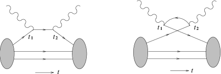
Figure 6: Time-ordered diagrams of the connected insertion involving quark and antiquark propagators between the currents.

A very important lattice observation is made in [66] that the SU(6) relation in the quark model is recovered in the valence approximation under which cloud quarks in the connected insertion are turned off. For example, the ratio $R_{A}=g^{0}_{\rm A,con}/g_{A}^{3}$ is found to be ${3\over 5}$ in the lattice calculation when the presence of cloud quarks and antiquarks is eliminated by disallowing quarks from propagating backward in time, while theoretically it is reduced under the valence approximation to $(\Delta u_{\rm con}+\Delta d_{\rm con})/(\Delta u_{\rm con}-\Delta d_{\rm con})$, which is equal to ${3\over 5}$ in the relativistic or non-relativistic quark model. Of course, the prediction $(g_{A}^{3})^{\rm NR}={5\over 3}$ in the non-relativistic quark model is too large compared to the experimental value $(g_{A}^{3})_{\rm expt}=1.2573\pm 0.0028$ [33]. Presumably, $(g_{A}^{3})^{\rm NR}$ is reduced by a factor of 3/4 due to relativistic effects. In other words, the above lattice observation implies that relativistic quark model results should be recovered in the valence approximation. Based on this observation, a picture for the smallness of $\Delta\Sigma_{\rm GI}$ or $g_{A}^{0}$ emerges. In the relativistic quark model, the non-relativistic SU(6) predictions $\Delta u^{\rm NR}={4\over 3}$ and $\Delta d^{\rm NR}=-{1\over 3}$ are reduced by the same factor to $\Delta u_{V}=1$ and $\Delta d_{V}=-{1\over 4}$, where the subscript “V” denotes a genuine valence spin component. Since the quark orbital angular momentum is nonvanishing in the presence of quark transverse momentum in the lower component of the Dirac spinor, the reduction of the spin component from $\Delta u^{\rm NR}+\Delta d^{\rm NR}=1$ to $\Delta u_{V}+\Delta d_{V}=0.75$ is shifted to the orbital component of the proton spin. Assuming SU(3)-symmetric sea polarization, as suggested by lattice calculations, one obtains from (2.26) that

$$\Delta u_{v}=\Delta u_{V}+\Delta u_{c}\simeq 0.93\,,~{}~{}~{}~{}\Delta d_{v}=\Delta d_{V}+\Delta d_{c}\simeq-0.33\,,$$ (6.3)

and hence

$$\Delta u_{c}\simeq-0.07\,,~{}~{}~{}~{}~{}\Delta d_{c}\simeq-0.08\,.$$ (6.4)

The cloud-quark polarization $\Delta q_{c}$ is thus negative in sign and comparable in magnitude to the sea polarization $\Delta q_{s}$. Now we have

$$\underbrace{\Delta u_{\rm GI}+\Delta d_{\rm GI}+\Delta s_{\rm GI}}_{0.30}=\underbrace{\Delta u_{V}+\Delta d_{V}}_{0.75}+\underbrace{\Delta u_{c}+\Delta d_{c}}_{-0.15}+\underbrace{\Delta u_{s}+\Delta d_{s}+\Delta s}_{-0.30}.$$ (6.5)

We conclude that the deviation of $\Delta\Sigma_{\rm GI}$ or $g_{A}^{0}$ from the relativistic quark model’s value 0.75 is ascribed to the negative cloud-quark and sea-quark polarizations. In the future, it will be of great importance to calculate $\Delta q_{V}$ and $\Delta q_{c}$ directly by lattice QCD.

The lattice results of [66] and [67] for $\Delta q_{\rm GI},~{}g_{A},~{}F$ and $D$ are presented in Table II; in general they agree with experiments within errors. Moments of polarized structure functions $g_{1}(x)$ and $g_{2}(x)$ from the connected insertion are reported in [99]. It is found that twist-3 operators characterized by the matrix element $d_{3}$ [cf. Eq.(4.18)] provide the dominant contribution to $\int^{1}_{0}x^{2}g_{2}(x)dx$.

Table II. Axial couplings and quark spin contents of the proton from lattice calculations and from experiments [see (2.19) and (2.26)].

	[66]	[67]	Experiment
$g_{A}^{0}$	0.25(12)	0.18(10)	0.31(7)
$g_{A}^{3}$	1.20(10)	0.985(25)	1.2573(28)
$g_{A}^{8}$	0.61(13)	—	0.579(25)
$\Delta u$	0.79(11)	0.638(54)	0.83(3)
$\Delta d$	-0.42(11)	-0.347(46)	-0.43(3)
$\Delta s$	-0.12(1)	-0.109(30)	-0.10(3)
$F$	0.45(6)	0.382(18)	0.459(8)
$D$	0.75(11)	0.607(14)	0.798(8)

As for the chiral-invariant quantity $\Delta\Sigma_{\rm CI}$, it involves the matrix element of $\tilde{J}^{+}_{5}$ in light-front gauge [see Eq.(4.57)] and hence sizeable gauge configurations are needed in lattice calculations for $\Delta\Sigma_{\rm CI}$. Nevertheless, it is conceivable to have lattice results for $\Delta G$ and $\Delta q_{\rm CI}$ soon in the near future.

6.2 Two-loop spin-dependent splitting functions

The experimental data of $g_{1}(x,Q^{2})$ taken at different $x$-bin correspond to different ranges of $Q^{2}$, that is, $Q^{2}$ of the data is $x$-bin dependent. To the zeroth order in QCD, $g_{1}$ simply reads $g_{1}(x)={1\over 2}\sum_{i}e^{2}_{i}\Delta q_{i}(x)$ without scaling violation. To the leading order (LO), it becomes $g_{1}(x,Q^{2})={1\over 2}\sum_{i}e^{2}_{i}\Delta q_{i}(x,Q^{2})$ with scaling violation arising from gluon bremsstrahlung and quark-antiquark pair creation from gluons. In other words, $\Delta G(x)$ enters into $g_{1}$ at LO only via the $Q^{2}$ evolution governed by the LO polarized AP equation. To the next-to-leading order (NLO), $g_{1}(x,Q^{2})$ is given by (3.1). At this order, gluons contribute directly to the polarized structure function $g_{1}$. A full NLO QCD analysis of the $g_{1}$ data is thus not possible until the two-loop splitting functions $\Delta P_{ij}^{(1)}(x)$ in the NLO $Q^{2}$ evolution equation are known. Since the complete results for $\Delta P_{ij}^{(1)}(x)$ are not available until very recently [52], all pre-1995 analyses based on the NLO expression (3.1) for $g_{1}(x,Q^{2})$ are not complete and fully consistent.

The $Q^{2}$ dependence of parton spin densities is determined by the spin-dependent Altarelli-Parisi equations:

$${d\over dt}\Delta q_{\rm NS}(x,t)=\,{\alpha_{s}(t)\over 2\pi}\Delta P_{qq}^{\rm NS}(x)\otimes\Delta q_{\rm NS}(x,t),$$

$${d\over dt}\left(\matrix{\Delta q_{\rm S}(x,t)\cr\Delta G(x,t)\cr}\right)=\,{\alpha_{s}(t)\over 2\pi}\left(\matrix{\Delta P_{qq}^{\rm S}(x)&2n_{f}\Delta P_{qG}(x)\cr\Delta P_{Gq}(x)&\Delta P_{GG}(x)\cr}\right)\otimes\left(\matrix{\Delta q_{\rm S}(x,t)\cr\Delta G(x,t)\cr}\right),$$ (6.6)

with $t=\ln(Q^{2}/\Lambda^{2}_{{}_{\rm QCD}})$,

$$\Delta q_{\rm NS}(x)=\Delta q_{i}(x)-\Delta q_{j}(x),~{}~{}~{}~{}~{}\Delta q_{\rm S}(x)=\sum_{i}\Delta q_{i}(x),$$ (6.7)

and

$$\Delta P_{ij}(x)=\Delta P_{ij}^{(0)}(x)+{\alpha_{s}\over 2\pi}\Delta P_{ij}^{(1)}(x)+\cdots.$$ (6.8)

The spin-dependent anomalous dimensions are defined as

$$\Delta\gamma_{ij}^{n}=\int^{1}_{0}\Delta P_{ij}(x)x^{n-1}dx=\Delta\gamma_{ij}^{(0),n}+{\alpha_{s}\over 2\pi}\Delta\gamma_{ij}^{(1),n}+\cdots.$$ (6.9)

The leading-order polarized splitting functions $\Delta P_{ij}^{(0)}$ are given by (3.26) and the corresponding anomalous dimensions for $n=1$ are

$$\Delta\gamma^{(0),1}_{qq}=\Delta\gamma^{(0),1}_{qG}=0,~{}~{}~{}\Delta\gamma^{(0),1}_{Gq}=2,~{}~{}~{}\Delta\gamma^{(0),1}_{GG}={1\over 2}{\beta_{0}},$$ (6.10)

where $\beta_{0}=11-2n_{f}/3$. To the NLO, $\Delta P_{qq}^{(1)}$ and $\Delta P_{qG}^{(1)}$ were calculated in the $\overline{\rm MS}$ scheme by Zijlstra and van Neerven [101]. However, the other two polarized splitting functions $\Delta P_{Gq}^{(1)}$ and $\Delta P_{GG}^{(1)}$ were not available until last year. The detailed results of $\Delta P_{ij}^{(1)}(x)$ are given in [52]. Here we just list the anomalous dimensions for $n=1$:

$$\Delta\gamma^{(1),1}_{{\rm NS},qq}=0,~{}~{}~{}~{}\Delta\gamma^{(1),1}_{{\rm S},qq}=-3C_{F}T_{f}=-2n_{f},$$

$$\Delta\gamma^{(1),1}_{qG}=0,~{}~{}~{}~{}\Delta\gamma^{(1),1}_{Gq}=-{1\over 8}\left(-6C_{F}^{2}-{142\over 3}C_{A}C_{F}+{8\over 3}C_{F}T_{f}\right)=25-{2\over 9}n_{f},$$ (6.11)

$$\Delta\gamma^{(1),1}_{GG}={\beta_{1}\over 4}=-{1\over 8}\left(-{68\over 3}C_{A}^{2}+8C_{F}T_{f}+{40\over 3}C_{A}T_{f}\right)={1\over 4}\left(102-{38\over 3}n_{f}\right),$$

where $C_{F}={4\over 3},~{}C_{A}=3,~{}T_{f}=n_{f}/2$. To this order,

$${\alpha_{s}\over 4\pi}=\,{1\over\beta_{0}\ln Q^{2}/\Lambda^{2}_{{}_{\overline{\rm MS}}}}-{\beta_{1}\ln\ln Q^{2}/\Lambda^{2}_{{}_{\overline{\rm MS}}}\over\beta_{0}^{3}(\ln Q^{2}/\Lambda^{2}_{{}_{\overline{\rm MS}}})^{2}}\,.$$ (6.12)

Note that the $\overline{\rm MS}$ regularization scheme is a gauge-invariant $k_{\perp}$-factorization scheme as it respects the axial anomaly in the triangle diagram. Therefore, the NLO evolution of parton spin distributions in the gauge-invariant factorization scheme is completely determined. Explicitly, the AP equation for the first moment of flavor-singlet parton spin densities reads

$${d\over dt}\left(\matrix{\Delta\Sigma_{\rm GI}(t)\cr\Delta G(t)\cr}\right)=\,{\alpha_{s}(t)\over 2\pi}\left(\matrix{{\alpha_{s}\over 2\pi}(-2n_{f})&0\cr 2+{\alpha_{s}\over 2\pi}(25-{2\over 9}n_{f})&{\beta_{0}\over 2}+{\alpha_{s}\over 2\pi}\,{\beta_{1}\over 4}\cr}\right)\left(\matrix{\Delta\Sigma_{\rm GI}(t)\cr\Delta G(t)\cr}\right).$$ (6.13)

Defining $\Delta\Gamma\equiv(\alpha_{s}/2\pi)\Delta G$, it is easily seen that

$${d\over dt}\left(\matrix{\Delta\Sigma_{\rm GI}(t)\cr\Delta\Gamma(t)}\right)=\left({\alpha_{s}\over 2\pi}\right)^{2}\left(\matrix{-2n_{f}&0\cr 2&0}\right)\left(\matrix{\Delta\Sigma_{\rm GI}(t)\cr\Delta\Gamma(t)}\right)+{\cal O}(\alpha_{s}^{3}),$$ (6.14)

which is in agreement with (4.64). A derivation of (6.14) does not need the information of $\Delta\gamma^{(1),1}_{Gq}$ and $\Delta\gamma^{(1),1}_{GG}$, however. The NLO $Q^{2}$ evolution of parton spin densities has been studied in [63, 102, 103, 104]. It is found that the difference between LO and NLO evolution for $\Delta\Sigma(x,Q^{2})$ and $\Delta G(x,Q^{2})$ is sizeable at small $x$, $x{\ \lower-1.2pt\vbox{\hbox{\hbox to0.0pt{$<$\hss}\lower 5.0pt\vbox{\hbox{$\sim$} }}}\ }5\times 10^{-3}$ (see Figs. 4 and 5 of [104]). This feature can be understood from the $x\to 0$ behavior of the splitting functions $\Delta P_{ij}(x)$. As $x\to 0$, we find from (3.26) that

$$\Delta P_{qq}^{(0)}\to{4\over 3},~{}~{}~{}\Delta P_{qG}^{(0)}\to-{1\over 2},~{}~{}~{}\Delta P_{Gq}^{(0)}\to{8\over 3},~{}~{}~{}~{}\Delta P_{GG}^{(0)}\to 12,$$ (6.15)

and from [52] that

$$\Delta P_{qq}^{(1)}\to\left(4C_{F}C_{A}-8C_{F}T_{f}-6C_{F}^{2}\right)\ln^{2}x=\,{16\over 3}(1-n_{f})\ln^{2}x,$$

$$\Delta P_{qG}^{(1)}\to-\left(2C_{A}+C_{F}\right)\ln^{2}x=-{22\over 3}\ln^{2}x,$$

$$\Delta P_{Gq}^{(1)}\to\left(8C_{A}C_{F}+4C_{F}^{2}\right)\ln^{2}x=\,{352\over 9}\ln^{2}x,$$ (6.16)

$$\Delta P_{GG}^{(1)}\to\left(16C_{A}^{2}-8C_{F}T_{f}\right)\ln^{2}x=\,{16\over 3}(27-n_{f})\ln^{2}x.$$

It is evident that for small enough $x$, the NLO $\Delta P_{ij}^{(1)}(x)$ can overcome the suppression factor $(\alpha_{s}/2\pi)$ and become comparable to the LO splitting functions.

6.3 Orbital angular momentum

We have discussed the operator definitions for $\Delta q$ and $\Delta G$ that are accessible with experiment in Sec. 4.5 and their $Q^{2}$ evolution in Secs. 3.3 and 4.6. It is natural to see if the similar analysis can be generalized to the orbital angular momenta of quarks and gluons. So far we have noticed two places where the orbital angular momentum plays a role. One is the compensation of the growth of $\Delta G$ with $Q^{2}$ by the angular momentum of the quark-gluon pair (see Sec. 4.3). The other is the reduction of the total spin component $\Delta\Sigma$ due to the presence of the quark transverse momentum in the lower component of the Dirac spinor is traded with the quark orbital angular momentum (see Sec. 6.1).

The generators associated with rotation invariance are

$$J^{\mu\nu}=\int d^{3}x\,M^{0\mu\nu},$$ (6.17)

where $M^{\alpha\mu\nu}$ is the angular momentum density given by (4.52). The first and third terms in (4.52) contribute to the quark and gluon orbital angular momentum, respectively. The angular momentum operator in QCD is related to the generators by

$$J^{i}=\,{1\over 2}\epsilon^{ijk}J^{jk}.$$ (6.18)

Explicitly [57],

$$J_{z}^{q} = S_{z}^{q}+L_{z}^{q}=\int d^{3}x\,[\,\bar{\psi}\gamma^{3}\gamma_{5}\psi+\psi^{\dagger}(\vec{x}\times i\vec{\partial})^{3}\psi],$$

$$J_{z}^{G} = S_{z}^{G}+L_{z}^{G}=\int d^{3}x\,[\,(\vec{E}\times\vec{A})^{3}-E_{i}(\vec{x}\times\vec{\partial})^{3}A_{i}].$$ (6.19)

Except for the quark helicity operator $S_{z}^{q}$, the other three operators $L_{z}^{q},~{}S_{z}^{G},~{}L_{z}^{G}$ are not separately gauge and Lorentz invariant. Very recently, Ji [105] has obtained gauge-invariant expressions:

$$L_{z}^{q}=\int d^{3}x\,\psi^{\dagger}(\vec{x}\times i\vec{D})^{3}\psi,~{}~{}~{}~{}J_{z}^{G}=\int d^{3}x\,\left[\vec{x}\times(\vec{E}\times\vec{B})\right]^{3}.$$ (6.20)

The gluon total angular momentum $J_{z}^{G}$ does not permit further gauge-invariant decomposition into spin and orbital pieces. However, in the infinite momentum frame and in the temporal axial gauge $A^{0}=0$, $S_{z}^{G}$ measures the gluon spin component $\Delta G$ which is accessible experimentally [cf. Eq.(4.54)]. As a result, the nucleon matrix element of $L_{z}^{G}$ in the infinite momentum frame and in $A^{0}=0$ gauge (or in the light-front coordinate and in light-front gauge) can be deduced from the matrix elements of $J_{z}^{G}$ and $S_{z}^{G}$ [105]. However, whether this definition of the gluon orbital angular momentum (and likewise $L_{z}^{q}$) contacts with experiment is still unknown.

The evolution of the quark and gluon orbital angular momenta was first discussed by Ratcliffe [106]. Using the operators given in (6.19), Ji, Tang and Hoodbhoy [53] recently have derived a complete leading-log evolution equation:

$${d\over dt}\left(\matrix{L_{z}^{q}\cr L_{z}^{G}\cr}\right)={\alpha_{s}(t)\over 2\pi}\left(\matrix{-{4\over 3}C_{F}&{n_{f}\over 3}\cr{4\over 3}C_{F}&-{n_{f}\over 3}\cr}\right)\left(\matrix{L_{z}^{q}\cr L_{z}^{G}\cr}\right)+{\alpha_{s}(t)\over 2\pi}\left(\matrix{-{2\over 3}C_{F}&{n_{f}\over 3}\cr-{5\over 6}C_{F}&-{11\over 2}\cr}\right)\left(\matrix{\Delta\Sigma\cr\Delta G\cr}\right),$$ (6.21)

with the solutions

$$L_{z}^{q}(Q^{2})=-{1\over 2}\Delta\Sigma+{1\over 2}\,{3n_{f}\over 16+3n_{f}}+f(Q^{2})\left(L_{z}^{q}(Q^{2}_{0})+{1\over 2}\Delta\Sigma-{1\over 2}\,{3n_{f}\over 16+3n_{f}}\right),$$

$$L_{z}^{G}(Q^{2})=-\Delta G(Q^{2})+{1\over 2}\,{16\over 16+3n_{f}}+f(Q^{2})\left(L_{z}^{G}(Q^{2}_{0})+\Delta G(Q^{2}_{0})-{1\over 2}\,{16\over 16+3n_{f}}\right),$$

where

$$f(Q^{2})=\left({\ln Q^{2}_{0}/\Lambda^{2}_{{}_{\rm QCD}}\over\ln Q^{2}/\Lambda^{2}_{{}_{\rm QCD}}}\right)^{{32+6n_{f}\over 33-2n_{f}}}$$ (6.23)

and $\Delta\Sigma$ is $Q^{2}$ independent to the leading-log approximation. We see that the growth of $\Delta G$ with $Q^{2}$ is compensated by the gluon orbital angular momentum, which also increases like $\ln Q^{2}$ but with opposite sign. The solution (6.22) has an interesting implication in the asymptotic limit $Q^{2}\to\infty$, namely

$$J_{z}^{q}(Q^{2})={1\over 2}\Delta\Sigma+L_{z}^{q}(Q^{2})\to~{}~{}~{}{1\over 2}\,{3n_{f}\over 16+3n_{f}}\,,$$

$$J_{z}^{G}(Q^{2})=\Delta G(Q^{2})+L_{z}^{G}(Q^{2})\to~{}~{}~{}{1\over 2}\,{16\over 16+3n_{f}}\,.$$ (6.24)

Thus, history repeats herself: The partition of the nucleon spin between quarks and gluons follows the well-known partition of the nucleon momentum. Taking $n_{f}=6$, we see that $J_{z}^{q}:J_{z}^{G}=0.53\,:\,0.47\,$. If the evolution of $J_{z}^{q}$ and $J_{z}^{G}$ is very slow, which is empirically known to be true for the momentum sum rule that half of the proton’s momentum is carried by gluons even at a moderate $Q^{2}$, then $\Delta\Sigma\sim 0.30$ at $Q^{2}=10\,{\rm GeV}^{2}$ implies that $L_{z}^{q}\sim 0.10$ at the same $Q^{2}$, recalling that the quark orbital angular momentum is expected to be of order 0.125 in the relativistic quark model.

Finally, it is worthy remarking that the spin sum rule

$${1\over 2}=\,{1\over 2}\Delta\Sigma_{\rm GI}+(L_{z}^{q})_{\rm GI}+\Delta G+L_{z}^{G}$$ (6.25)

so far is defined in the gauge-invariant $k_{\perp}$-factorization scheme. In the chiral-invariant scheme we have $\Delta\Sigma_{\rm CI}=\Delta\Sigma_{\rm GI}+(n_{f}\alpha_{s}/2\pi)\Delta G$, but $g_{1}(x)$ and $\Gamma_{1}$ remain unchanged [cf. Eq.(4.38)]. Since $\Delta G$ and $L_{z}^{G}$ are independent of the $k_{\perp}$-factorization, a replacement of $\Delta\Sigma_{\rm GI}$ by $\Delta\Sigma_{\rm CI}$ in the spin sum rule (6.25) requires that the difference $\Delta\Sigma_{\rm CI}-\Delta\Sigma_{\rm GI}=(n_{f}\alpha_{s}/2\pi)\Delta G$ be compensated by a counterpart in the gluon orbital angular momentum; that is,

$$(L_{z}^{q})_{\rm CI}=(L_{z}^{q})_{\rm GI}-{n_{f}\alpha_{s}\over 4\pi}\Delta G.$$ (6.26)

This relation also can be visualized as follows (see [53]). Suppose we first work in the chiral-invariant scheme and consider a gluon with +1 helicity splitting into a massless quark-antiquark pair. The total helicity of the gluon is entirely transferred to the orbital angular momentum of the pair due to helicity conservation or chiral symmetry. Now, shifting the axial anomaly from the hard part of the photon-gluon box diagram to the triangle diagram so that a negative sea-quark polarization is produced via the anomaly mechanism [see Eqs.(4.29)-(4.32)]. In order to preserve the total angular momentum, this sea-quark polarization must be balanced by the same amount of the quark orbital angular momentum induced from the anomaly. It is interesting to note that when $\Delta G$ is of order 2.5 , one will have $\Delta\Sigma_{\rm CI}\sim 0.60$ [cf. Eq.(3.31)] but $(L_{z}^{q})_{\rm CI}\sim-0.05$ . In other words, while $\Delta\Sigma_{\rm CI}$ is close to the quark-model value, $(L_{z}^{q})_{\rm CI}$ deviates more from the quark model and even becomes negative !

7 Polarized Parton Distribution Functions

7.1 Prelude

One of the main goals in the study of polarized hadron structure functions measured in DIS is to determine the spin-dependent valence-quark, cloud-quark, sea-quark and gluon distributions and to understand the spin structure of the nucleon. In spite of the recent remarkable progress in polarized DIS experiments, the extraction of spin-dependent parton distribution functions, especially for sea quarks and gluons, from the measured polarized hadron structure functions remains largely ambiguous and controversial. We shall see that a full NLO analysis of the $g_{1}(x,Q^{2})$ data just became possible recently and it indicates that the sea-quark and gluon spin distributions are, to a large degree, still unconstrained by current experimental data. Nevertheless, we are entering the phase of having the parton spin densities parametrized and determined to the NLO.

In general the polarized proton structure function $g_{1}(x,Q^{2})$ has the form [101]

$$g_{1}(x,Q^{2}) = {1\over 2}\sum_{q}^{n_{f}}e^{2}_{q}\Bigg{\{}\Delta q(x,\mu_{\rm fact}^{2})+{\alpha_{s}(\mu_{\rm fact}^{2})\over 2\pi}\Big{[}\Delta C^{\rm S}_{q}(x,Q^{2},\mu_{\rm fact}^{2})\otimes\Delta q_{\rm S}(x,\mu_{\rm fact}^{2})$$

$$+~{}\Delta C^{\rm NS}_{q}(x,Q^{2},\mu_{\rm fact}^{2})\otimes\Delta q_{\rm NS}(x,\mu_{\rm fact}^{2})+\Delta C_{G}(x,Q^{2},\mu_{\rm fact}^{2})\otimes\Delta G(x,\mu_{\rm fact}^{2})\Big{]}\Bigg{\}},$$

with

$$\Delta C_{q,G}(x)=\,\Delta C_{q,G}^{(0)}(x)+{\alpha_{s}\over 2\pi}\Delta C_{q,G}^{(1)}(x)+\cdots.$$ (7.2)

Note that $(\alpha_{s}/2\pi)\Delta C_{G}(x)$ is equal to the hard photon-gluon cross section $\Delta\sigma^{\gamma G}_{\rm hard}(x)$ in (3.1) and $\otimes$ denotes convolution. The gluon coefficient function $\Delta C_{G}(x)$ and the quark spin density $\Delta q(x)$ depend on the $k_{\perp}$-factorization scheme, while the quark coefficient function $\Delta C_{q}(x)$ depends on the regularization scheme chosen. In the $\overline{\rm MS}$ scheme, which is also a gauge-invariant factorization scheme, $\Delta C_{{\rm S},q}^{(0)}(x,Q^{2})=\Delta C_{{\rm NS},q}^{(0)}(x,Q^{2})=\Delta f_{q}(x,Q^{2})$ [cf. Eq.(3.3)] and

$$\Delta C_{G}^{(0)}(x,Q^{2},\mu_{\rm fact}^{2})_{\rm GI}=\,(2x-1)\left(\ln{Q^{2}\over\mu_{\rm fact}^{2}}+\ln{1-x\over x}-1\right)+2(1-x)$$ (7.3)

and the NLO $\Delta C_{q,G}^{(1)}$ are given in [101]. In the chiral-invariant scheme, the leading order $\Delta C_{G}(x)$ is calculated to be [cf. Eq.(3.20)]

$$\Delta C_{G}^{(0)}(x,Q^{2},\mu_{\rm fact}^{2})_{\rm CI}=\,(2x-1)\left(\ln{Q^{2}\over\mu_{\rm fact}^{2}}+\ln{1-x\over x}-1\right).$$ (7.4)

The first moments of the coefficient functions are

$$\int^{1}_{0}\Delta C_{q}^{(0)}(x)_{\rm GI}=-2,~{}~{}~{}\int^{1}_{0}\Delta C_{G}^{(0)}(x)_{\rm GI}=0,~{}~{}~{}\int^{1}_{0}\Delta C_{G}^{(0)}(x)_{\rm CI}=-1.$$ (7.5)

The $Q^{2}$ dependence of the parton spin densities is determined by the AP equation (6.6). As mentioned in Sec. 6.2, at the zeroth order of $\alpha_{s}$, $\Delta C_{q,G}(x)=0$ and $\Delta P_{ij}(x)=0$. At NLO we still have $\Delta C_{q,G}(x)=0$ but $\Delta P_{ij}^{(0)}(x)\neq 0$; that is, there is a scaling violation in $g_{1}(x,Q^{2})$ but $\Delta G(x)$ enters indirectly via the $Q^{2}$ evolution. A complete NLO analysis of $g_{1}(x,Q^{2})$ requires the information of $\Delta P_{ij}^{(1)}(x)$ in addition to $\Delta C_{q,G}^{(0)}(x)$. At this order, gluons start to contribute directly to the polarized structure function. For a next-to-next-to-leading order description we have to await three-loop results for $\Delta P_{ij}^{(2)}(x)$, although $\Delta C_{q,G}^{(1)}(x)$ have been calculated.

Several remarks are in order.

• It is clear from (7.1) that with the input of parton spin distributions at $Q^{2}=\mu_{\rm fact}^{2}$, the $Q^{2}$ evolution is governed by the logarithmic term $\ln(Q^{2}/\mu_{\rm fact}^{2})$ in the coefficient functions, as long as $\alpha_{s}(\mu_{\rm fact}^{2})\ln(Q^{2}/\mu_{\rm fact}^{2})<<1$. For $Q^{2}>>\mu_{\rm fact}^{2}$, the logarithmic terms have to be resummed using renormalization group methods [101]. For a fixed $\mu_{\rm fact}^{2}$ and for $Q^{2}$ not deviating too much from $\mu_{\rm fact}^{2}$, the $\ln(Q^{2}/\mu_{\rm fact}^{2})$ terms in $\Delta C_{q,G}^{(0)}$ give rise to the leading-log (LL) $Q^{2}$ evolution to $g_{1}(x,Q^{2})$, and the $\ln^{2}(Q^{2}/\mu_{\rm fact}^{2})$ terms in $\Delta C_{q,G}^{(1)}$ determine the $Q^{2}$ dependence to the next-to-leading log (NLL) approximation. When $\mu_{\rm fact}^{2}$ is set to be $Q^{2}$, the $\ln(Q^{2}/\mu_{\rm fact}^{2})$ terms appearing in coefficient functions are equal to zero and (7.1) becomes

  $$g_{1}(x,Q^{2}) = {1\over 2}\sum_{q}^{n_{f}}e^{2}_{q}\Bigg{\{}\Delta q(x,Q^{2})+{\alpha_{s}(Q^{2})\over 2\pi}\Big{[}\Delta C^{\rm S}_{q}(x,\alpha_{s})\otimes\Delta q_{\rm S}(x,Q^{2})$$ (7.6)

  $$+ \Delta C^{\rm NS}_{q}(x,\alpha_{s})\otimes\Delta q_{\rm NS}(x,Q^{2})+\Delta C_{G}(x,\alpha_{s})\otimes\Delta G(x,Q^{2})\Big{]}\Bigg{\}}.$$

  In this case, the $Q^{2}$ evolution of $g_{1}(x,Q^{2})$ is taken over by the parton spin distributions. Using $F_{2}(x,Q^{2})$ as a testing example, it is shown explicitly in [101] that the $Q^{2}$ dependence determined by the LL (NLL) parametrization of parton densities in which LL (NLL) logs are resummed to all orders of perturbation theory is indeed consistent with the leading (next-to-leading) $Q^{2}$ evolution obtained from fixed order perturbation theory (i.e., $\mu_{\rm fact}$ being kept fixed). In short, generally we have to solve the spin-dependent AP equation (6.6) to determine the $Q^{2}$ dependence of spin-dependent parton distributions and hence the $Q^{2}$ evolution of $g_{1}$ via (7.6). However, for $Q^{2}$ not deviating too much from $\mu_{\rm fact}^{2}$, (7.1) provides a good approximation to the $Q^{2}$ evolution of $g_{1}(x,Q^{2})$ through the $\ln(Q^{2}/\mu_{\rm fact}^{2})$ terms in coefficient functions.

• Although the contribution $\Delta C_{G}\otimes\Delta G$ in (7.1) or (7.6) is formally of order $\alpha_{s}$, it actually does not vanish in the asymptotic limit due to the axial anomaly. It is thus expected that the NLO corrections to sea-quark and gluon spin distributions are important.

• Before the availability of the two-loop splitting functions $\Delta P_{ij}^{(1)}(x)$, some analyses of $g_{1}(x,Q^{2})$ were strictly done at the leading order, namely $g_{1}(x,Q^{2})={1\over 2}\sum e_{q}^{2}\Delta q(x,Q^{2})$ with the gluon-spin effects entering via the $Q^{2}$ evolution (see e.g., [107, 45]). As $\alpha_{s}(Q^{2})\Delta G(Q^{2})$ is of order $\alpha_{s}^{0}$, several analyses have been performed using a hybrid expression for $g_{1}$

  $$g_{1}(x,Q^{2})=\,{1\over 2}\sum e^{2}_{q}\left[\Delta q(x,Q^{2})+{\alpha_{s}\over 2\pi}\,\Delta C_{G}(x)\otimes\Delta G(x,Q^{2})\right]$$ (7.7)

  in the chiral-invariant factorization scheme. However, the gluon coefficient function employed in many earlier studies is often incorrect. For example, $\Delta C_{G}^{\rm CI}(x)=-\delta(1-x)$ was used in [108] and $\Delta C_{G}^{\rm CI}(x)=(2x-1)\ln[(1-x)/x]$ in [109, 110].

• In spite of the fact that the combination $\Delta q(x,\mu_{\rm fact})+(\alpha_{s}(\mu_{\rm fact})/2\pi)\Delta C_{G}\otimes\Delta G(x,\mu_{\rm fact}^{2})$ in (7.1) is $k_{\perp}$-factorization independent [see Eqs.(4.33) and (4.37)], the lack of knowledge on the splitting functions $\Delta P_{ij}^{(1)}(x)$ in the chiral-invariant scheme indicates that, in practice, we should work entirely in the gauge-invariant factorization scheme in which hard gluons do not make contributions to $\Gamma_{1}$. This is further reinforced by the observation that in the literature most of NLO parametrizations of unpolarized parton distributions, which are needed to satisfy the positivity constraints $|\Delta q(x,Q^{2})|\leq q(x,Q^{2})$ and $|\Delta G(x,Q^{2})|\leq G(x,Q^{2})$, are performed in the $\overline{\rm MS}$ scheme.

7.2 Constraints on polarized parton distributions

As stressed in Sec. 6.1, the quark spin density $\Delta q(x)$ consists of valence-quark, cloud-quark and sea-quark components: $\Delta q_{V}(x),~{}\Delta q_{c}(x)$ and $\Delta q_{s}(x)$. Unfortunately, there is no any experimental and theoretical guidelines on the shape of the spin-dependent cloud-quark distribution, though it is argued in Sec. 6.1 that the cloud-quark polarization is comparable to sea-quark polarization in sign and magnitude. Since the spin component of cloud quarks originates from valence quarks (there is no cloud strange quark), we will proceed by considering the combination $\Delta q_{v}(x)=\Delta q_{V}(x)+\Delta q_{c}(x)$, which is commonly (but not appropriately) referred to as the “valence” quark contribution. Since the sea polarization is found to be SU(3)-flavor symmetric empirically in lattice calculations [66, 67], we will make the plausible assumption of SU(3)-symmetric sea-quark spin components. This assumption is justified since the disconnected insertions from which the sea-quark spin component originates are dominated by the triangle diagram and hence are independent of the light quark masses in the loop. Therefore, for SU(3)-symmetric sea polarization, we obtain from (2.26) that $\Delta u_{v}=\,0.93\,,~{}\Delta d_{v}=-0.33$ at $Q^{2}=10\,{\rm GeV}^{2}$ [cf. Eq.(6.3)]. As explained in Sec. 6.1, the deviation of the result $\Delta u_{v}+\Delta d_{v}=0.60$ from the relativistic quark model’s prediction $\Delta u_{V}+\Delta d_{V}=0.75$ stems from the negative cloud-quark polarization.

The valence quark spin density at $x\to 1$ is subject to a model-independent constraint. According to the perturbative QCD argument [111], the valence quarks at $x=1$ remember the spin of the parent proton, i.e., $\Delta u_{v}(x)/u_{v}(x),~{}\Delta d_{v}(x)/d_{v}(x)\to 1$ as $x\to 1$, as originally conjectured by Feynman [112]. Since $\Delta d_{v}$ is negative while $\Delta d_{v}(x)$ is positive as $x\to 1$, it means that the sign of $\Delta d_{v}(x)$ flips somewhere between $0<x<1$ [113]. A model for valence-quark spin distributions has been proposed sometime ago by Carlitz and Kaur [114]. According to this model, $\Delta d_{v}(x)/d_{v}(x)\to-{1\over 3}$ as $x\to 1$, which disagrees with what expected from perturbative QCD. Experimentally, it is possible to carry out a straightforward measurement of the ratio $\Delta d_{v}(x)/d_{v}(x)$ to test various predictions by measuring the longitudinal spin asymmetry in the inclusive $W^{-}$ production in proton-proton collisions [115]. This spin asymmetry is proportional to $\Delta d_{v}(x)/d_{v}(x)$ in the appropriate kinematic range (see Sec. 8).

In terms of valence and sea spin distributions, $g_{1}^{p}$ can be recast to the form

$$g_{1}^{p}(x,Q^{2}) = {1\over 2}\int^{1}_{x}{dy\over y}\Bigg{\{}\left[{4\over 9}\Delta u_{v}(y,Q^{2})+{1\over 9}\Delta d_{v}(y,Q^{2})+{2\over 3}\Delta s(y,Q^{2})\right]$$

$$\times \left[\delta\left(1-{x\over y}\right)+{\alpha_{s}(Q^{2})\over 2\pi}\Delta C_{q}^{(0)}(x/y)\right]+{\alpha_{s}(Q^{2})\over 6\pi}\,\Delta C_{G}^{(0)}(x/y)\Delta G(y,Q^{2})\Bigg{\}}.$$

In general, both sea quarks and gluons contribute to $g_{1}^{p}(x)$. Since the unpolarized sea distribution and the unpolarized gluon distribution multiplied by $\alpha_{s}/(6\pi)$ are small at $x{\ \lower-1.2pt\vbox{\hbox{\hbox to0.0pt{$>$\hss}\lower 5.0pt\vbox{\hbox{$\sim$} }}}\ }0.2$, the positivity constraints $|\Delta s(x)|\leq s(x)$ and $|\Delta G(x)|\leq G(x)$ imply that the data of $g_{1}^{p}(x)$ at $x{\ \lower-1.2pt\vbox{\hbox{\hbox to0.0pt{$>$\hss}\lower 5.0pt\vbox{\hbox{$\sim$} }}}\ }0.2$ should be almost accounted for by $\Delta u_{v}(x)$ and $\Delta d_{v}(x)$. Therefore, the shape of the spin-dependent valence quark densities is nicely restricted by the measured $g_{1}^{p}(x)$ at $x{\ \lower-1.2pt\vbox{\hbox{\hbox to0.0pt{$>$\hss}\lower 5.0pt\vbox{\hbox{$\sim$} }}}\ }0.2\,$ together with the first-moment constraint (6.3) and the perturbative QCD requirement that $\Delta q_{v}(x)/q_{v}(x)\to 1$ at $x=1$. In order to ensure the validity of the positivity condition $|\Delta q_{v}(x)|\leq q_{v}(x)$, we choose the NLO Martin-Roberts-Stirling MRS(A^′) set [117] parametrized in the $\overline{\rm MS}$ scheme at $Q^{2}=4\,{\rm GeV}^{2}$ as unpolarized valence quark distributions:

$$u_{v}(x,Q^{2}=4\,{\rm GeV}^{2}) = 2.26\,x^{-0.441}(1-x)^{3.96}(1-0.54\sqrt{x}+4.65x),$$

$$d_{v}(x,Q^{2}=4\,{\rm GeV}^{2}) = 0.279\,x^{-0.665}(1-x)^{4.46}(1+6.80\sqrt{x}+1.93x).$$ (7.9)

Accordingly, we must employ the same $\overline{\rm MS}$ scheme for polarized parton distributions in order to apply the positivity constraint. For the spin-dependent valence distributions we assume that they have the form [44]

$$\Delta q_{v}(x)=\,x^{\alpha}(1-x)^{\beta}(a+b\sqrt{x}+cx+dx^{1.5}),$$ (7.10)

with $\alpha$ and $\beta$ given by Eq.(7.9). We find that an additional term proportional to $x^{1.5}$ is needed in (7.10) in order to satisfy the above three constraints.

For the data of $g_{1}^{p}(x)$, we will use the SMC [27] and EMC [7] results, both being measured at the mean value of $Q^{2}_{0}=10\,{\rm GeV}^{2}$. Following the SMC analysis we have used the new $F_{2}(x)$ structure function measured by NMC [118], which has a better accuracy at low $x$, to update the EMC data. Assuming that $Q^{2}=\langle Q^{2}_{0}\rangle=10\,{\rm GeV}^{2}$ for each $x$ bin of the $g_{1}(x,Q^{2})$ data, a best least $\chi^{2}$ fit to $g_{1}^{p}(x)$ at $x{\ \lower-1.2pt\vbox{\hbox{\hbox to0.0pt{$>$\hss}\lower 5.0pt\vbox{\hbox{$\sim$} }}}\ }0.2$ by (7.10) is found to be [44]

$$\Delta u_{v}(x,Q^{2}_{0}) = x^{-0.441}(1-x)^{3.96}(0.928+0.149\sqrt{x}-1.141x+11.612x^{1.5}),$$

$$\Delta d_{v}(x,Q^{2}_{0}) = x^{-0.665}(1-x)^{4.46}(-0.038-0.43\sqrt{x}-5.260x+8.443x^{1.5}),$$ (7.11)

which satisfies all aforementioned constraints. Note that we have evoluted $q_{v}(x,Q^{2})$ from $Q^{2}=4\,{\rm GeV}^{2}$ to $10\,{\rm GeV}^{2}$ in order to compare with $\Delta q_{v}(x,Q^{2}_{0})$ and that the sign of $\Delta d_{v}(x)$ in our parametrization flips at $x_{0}=0.496\,$ (see Fig. 7).

The NLO parametrization (7.11) for valence quark spin densities is obtained by assuming $Q^{2}=\langle Q^{2}_{0}\rangle$ for each $x$ bin of the $g_{1}(x,Q^{2})$ data. However, a full NLO analysis should take into account the measured $x$ dependence of $Q^{2}$ at each $x$ bin by considering the NLO evolution of parton spin distributions. At present, there already exist several such analyses [63, 102, 103, 104]. For example, by fitting some parametrizations for spin-dependent parton distributions to all available world data on $g_{1}(x,Q^{2})$, Gehrmann and Stirling [103] obtained (set A)

$$\Delta u_{v}(x,Q^{2}) = 0.918A_{u}\,x^{-0.488}(1-x)^{3.96}(1-4.60\sqrt{x}+11.65x),$$

$$\Delta d_{v}(x,Q^{2}) = -0.339A_{d}\,x^{-0.220}(1-x)^{4.96}(1-3.48\sqrt{x}+7.81x),$$ (7.12)

to NLO at $Q^{2}=4\,{\rm GeV}^{2}$, where $A_{u}=1.3655$ and $A_{d}=3.8492$ are normalization factors ensuring that the first moments of $\Delta u_{v}(x)$ and $\Delta d_{v}(x)$ are 0.918 and $-0.339$, respectively. However, the $x\to 1$ behavior of the valence quark spin distributions (7.12) : $\Delta u_{v}(x)/u_{v}(x)\to 0.87$ and $\Delta d_{v}(x)/d_{v}(x)\to-2.56$ is not consistent with above-mentioned QCD constraint (the latter also seems to violate the positivity constraint). Three different NLO parametrizations of valence quark spin distributions are shown in Fig. 7.

Figure 7: NLO valence-quark spin distributions at $Q^{2}=10\,{\rm GeV}^{2}$ for three different parametrizations: (7.11) (thick solid curve denoted by CLW [44]), the standard set of GRSV [102] (solid curve) and set A of GS [103] (dotted curve).

A comparison between the theoretical curve of $xg_{1}^{p}(x)$ fitted to the EMC and SMC data at $x{\ \lower-1.2pt\vbox{\hbox{\hbox to0.0pt{$>$\hss}\lower 5.0pt\vbox{\hbox{$\sim$} }}}\ }0.2$ with the polarized valence quark distribution given by (7.11) is shown in Fig. 1 (see Sec. 2.2). The discrepancy between theory and experiment for $g_{1}^{p}(x)$ at small $x$ is presumably accounted for by sea quarks and gluons. For sea-quark polarization, we know that its size is of order $-0.10$, but there is no any information on the size of gluon polarization. The sea-quark and gluon spin distributions cannot be separately determined by current experimental data [103, 102]; they are correlatively constrained by (7.8). In other words, while the shapes of the spin-dependent valence quark distributions are fairly constrained by the data, the sea-quark and gluon spin densities are almost completely undetermined. In principle, measurements of scaling violation in $g_{1}(x,Q^{2})$ via, for example, the derivative of $g_{1}(x,Q^{2})$ with respect to $Q^{2}$, in next-generation experiments will allow an estimate of the gluon spin density and the overall size of gluon polarization. Of course, the data should be sufficiently accurate in order to study the gluon spin density. Meanwhile, it is even more important to probe $\Delta G(x)$ independently in those hadron-hadron collision processes where gluons play a dominant role (see Sec. 8).

As stressed in passing, the fact that gluons make no contributions to $\Gamma_{1}$ in the gauge-invariant factorization scheme does not imply a vanishing gluon contribution to $g_{1}(x)$. Quite opposite to the naive sea-quark interpretation for $g_{1}(x)$, if there is no sea polarization in the chiral-invariant scheme, then the size of the gluon spin component in a proton must numerically obey the relation $\Delta G(Q^{2})=-(2\pi/\alpha_{s}(Q^{2}))\Delta q_{s}^{\rm GI}(Q^{2})$ [cf. Eq.(4.37)] in order to perturbatively generate a negative sea-quark polarization $\Delta q_{s}^{\rm CI}(Q^{2})$ via the anomaly mechanism. In other words, even gluons do not contribute to $\Gamma_{1}^{p}$, the gluon spin can be as large as 2.5 for $\Delta q_{s}^{\rm GI}=-0.10\,$ at $Q^{2}=10\,{\rm GeV}^{2}$ provided that $\Delta q_{s}^{\rm CI}=0$. Recall that the gluon polarization induced from quark’s bremsstrahlung is positive [cf. Eq.(3.29)]. Recently, a full NLO analysis was performed in the chiral-invariant factorization scheme [63] and it was claimed that the present data of $g_{1}$ are sufficient to determine the first moment of the gluon spin distribution, namely $\Delta G(Q^{2}=1\,{\rm GeV}^{2})=1.5\pm 0.8$ and is roughly twice as large at $Q^{2}=10\,{\rm GeV}^{2}$. Since the shape and size of the spin-dependent gluon distribution is $k_{\perp}$-factorization independent, evidently there is a contradiction between the conclusions of [63] and of [102, 103]. Because $\Delta P_{ij}^{(1)}(x)$ and $\Delta C_{q}^{(1)}(x)$ are available only in the $\overline{\rm MS}$ scheme, it has been attempted to introduce a modification on NLO anomalous dimensions and hard coefficient functions to transfer from the GI scheme to the CI prescription [101]. In the CI scheme, $\Delta\Sigma_{\rm CI}$ does not evolve with $Q^{2}$ and this requires that

$$\int^{1}_{0}\Delta C_{G}^{(1)}(x)_{\rm CI}dx=-1,~{}~{}~{}~{}\Delta\gamma_{{\rm S},qq}^{(1),1}=0.$$ (7.13)

However, this transformation cannot be unique since it is only subject to the constraints (7.13). Indeed, three different scheme changes have been constructed in [63]. As a consequence, the NLO evolution of polarized parton distributions in the CI scheme obtained in this manner [63] is ambiguous as it depends on the scheme of transformation.

Finally, the interested reader is referred to [119] for a collection of polarized parton distributions up to 1995.

8 Experimental Signatures of Parton Polarizations

It is concluded in Sec. 7.2 that while the present experimental data put a useful constraint on the shape of the valence-quark spin distributions, the sea-quark and gluon spin densities are only loosely constrained. The question of what is the magnitude and even the sign of the gluon spin remains unanswered. In view of this, we shall survey the processes which can be used to probe the parton spin densities, especially for sea quarks and gluons. For the purposes of this section, we will use $\Delta q$ and $\Delta\bar{q}$ to denote the spin components of quarks and antiquarks, respectively.

valence-quark spin distribution $\Delta q_{v}(x)$ $\bullet$ semi-inclusive DIS [120, 121, 122]  Consider the semi-inclusive decays $\vec{e}+\vec{p}\to e+(\pi^{\pm},K^{\pm},K^{0},$$\bar{K}^{0})+X$ with the longitudinally polarized lepton beam and proton target. The differential cross section for the production of a hadron in DIS of charged lepton has the form

$${d^{3}\sigma\over dxdydz}\sim{dN^{h}\over dz}\,\propto\,\sum_{i=q,\bar{q}}e^{2}_{i}q_{i}(x,Q^{2})D_{i}^{h}(z,Q^{2}),$$ (8.1)

where $y=\nu/E=(E-E^{\prime})/E$, $z$ is the fraction of the parent parton’s momentum carried by the final hadron $h$, $N^{h}$ is the number of hadrons produced with a value of $z$, and $D_{i}^{h}$ is the fragmentation function of a quark $i$ into the hadron $h$. Therefore,

$${dN^{h}_{\uparrow\downarrow}\over dz}-{dN^{h}_{\uparrow\uparrow}\over dz}\,\propto\,\sum e^{2}_{i}\Delta q_{i}(x,Q^{2})D^{h}_{i}(z,Q^{2}).$$ (8.2)

Based on (8.2), two semi-inclusive asymmetries of interest are

$${\cal A}^{h}(x,Q^{2})=\,{N^{h}_{\uparrow\downarrow}-N^{h}_{\uparrow\uparrow}\over N^{h}_{\uparrow\downarrow}+N^{h}_{\uparrow\uparrow}}=\,{\sum e^{2}_{i}\Delta q_{i}(x,Q^{2})D_{i}^{h}(Q^{2})\over\sum e^{2}_{i}q_{i}(x,Q^{2})D^{h}_{i}(Q^{2})},$$ (8.3)

where $D^{h}_{i}(Q^{2})=\int^{1}_{0}dz\,D^{h}_{i}(z,Q^{2})$, and

$${\cal A}^{h^{+}-h^{-}}(x,z,Q^{2})=\,{dN^{h^{+}-h^{-}}_{\uparrow\downarrow}/dz-dN^{h^{+}-h^{-}}_{\uparrow\uparrow}/dz\over dN^{h^{+}-h^{-}}_{\uparrow\downarrow}/dz+dN^{h^{+}-h^{-}}_{\uparrow\uparrow}/dz}.$$ (8.4)

It follows that the asymmetries in difference of deep inelastic $\pi^{+}$ and $\pi^{-}$ productions given by

$${\cal A}_{p}^{\pi^{+}-\pi^{-}}(x,Q^{2})=\,{4\Delta u_{v}(x,Q^{2})-\Delta d_{v}(x,Q^{2})\over 4u_{v}(x,Q^{2})-d_{v}(x,Q^{2})}$$ (8.5)

for the proton target, and

$${\cal A}_{d}^{\pi^{+}-\pi^{-}}(x,Q^{2})=\,{\Delta u_{v}(x,Q^{2})+\Delta d_{v}(x,Q^{2})\over u_{v}(x,Q^{2})+d_{v}(x,Q^{2})}$$ (8.6)

for the deuteron target, are completely independent of the fragmentation function and can be used to extract the polarized valence quark densities. Likewise, for kaon production

$${\cal A}^{K^{+}-K^{-}}_{p}(x,Q^{2})=\,{\Delta u_{v}(x,Q^{2})\over u_{v}(x,Q^{2})},~{}~{}~{}~{}~{}{\cal A}^{K^{0}-\bar{K}^{0}}_{p}(x,Q^{2})=\,{\Delta d_{v}(x,Q^{2})\over d_{v}(x,Q^{2})}.$$ (8.7)

A measurement of the asymmetry in difference of $K^{0}$ and $\bar{K}^{0}$ productions is thus very useful to test the large $x$ behavior of $\Delta d_{v}(x)/d_{v}(x)$, which is expected to approach unity in perturbative QCD, but to $-{1\over 3}$ according to the Carlitz-Kaur model [114]. Theoretically, NLO corrections to semi-inclusive asymmetries were recently studied in [122]. Experimentally, asymmetries ${\cal A}_{p,d}^{\pi}$ and ${\cal A}_{p,d}^{\pi^{+}-\pi^{-}}$ have been measured by SMC recently [36], from which valence quark and non-strange quark spin distributions are extracted with the results: $\Delta u_{v}=1.01\pm 0.19\pm 0.14$ and $\Delta d_{v}=-0.57\pm 0.22\pm 0.11\,$.

$\bullet$ $W^{\pm}$ and $Z$ production [123, 124]  In high-energy hadron-hadron collisions, the single-spin asymmetry ${\cal A}_{L}$ defined by

$${\cal A}_{L}=\,{d\sigma^{\uparrow}-d\sigma^{\downarrow}\over d\sigma^{\uparrow}+d\sigma^{\downarrow}},$$ (8.8)

with $d\sigma^{\uparrow(\downarrow)}$ denoting the inclusive cross section where one of the initial hadron beams is longitudinally polarized and has $+(-)$ helicity, is expected to vanish to all orders in strong interactions unless some of the parton-parton scatterings involve parity-violating weak interactions. Therefore, a nonzero ${\cal A}_{L}$ arises from the interference between strong and weak amplitudes and usually is small, of order $10^{-4}$ (for a recent analysis of parity-violating asymmetries, see [125, 126]). The only exception is the direct $W^{\pm}$ and $Z$ productions in proton-proton collisions where a large ${\cal A}_{L}$ of order 10% is expected to be seen at RHIC energies [124]. In the parton model, $p\vec{p}\to W^{\pm}+X$ proceeds dominantly via $u\bar{d}\to W^{+}~{}(\bar{u}d\to W^{-})$

$${\cal A}_{L}^{W^{+}} = {\Delta u(x_{a},M_{W}^{2})\bar{d}(x_{b},M_{W}^{2})-\Delta\bar{d}(x_{a},M_{W}^{2})u(x_{b},M_{W}^{2})\over u(x_{a},M_{W}^{2})\bar{d}(x_{b},M_{W}^{2})+\bar{d}(x_{a},M_{W}^{2})u(x_{b},M_{W}^{2})},$$

$${\cal A}_{L}^{W^{-}} = {\Delta d(x_{a},M_{W}^{2})\bar{u}(x_{b},M_{W}^{2})-\Delta\bar{u}(x_{a},M_{W}^{2})d(x_{b},M_{W}^{2})\over d(x_{a},M_{W}^{2})\bar{u}(x_{b},M_{W}^{2})+\bar{u}(x_{a},M_{W}^{2})d(x_{b},M_{W}^{2})},$$ (8.9)

where $x_{a}=\sqrt{\tau}\exp(y),~{}x_{b}=\sqrt{\tau}\exp(-y),~{}\tau=M^{2}_{W}/s$. As $y$ is near 1, we have $x_{a}>>x_{b}$ and

$${\cal A}_{L}^{W^{+}}\sim\,{\Delta u(x_{a},M^{2}_{W})\over u(x_{a},M_{W}^{2})},~{}~{}~{}~{}{\cal A}_{L}^{W^{-}}\sim\,{\Delta d(x_{a},M^{2}_{W})\over d(x_{a},M_{W}^{2})},$$ (8.10)

where $x_{a}=e\sqrt{\tau}$. The (valence) quark spin distributions at large $x$ and at $Q^{2}=M^{2}_{W}$ thus can be determined at the kinematic limit $y\sim 1$.

antiquark and sea-quark distributions $\Delta\bar{q}(x),~{}\Delta q_{s}(x)$ $\bullet$ semi-inclusive DIS [120, 129]  Assuming $D^{\pi^{+}}_{u}(z)>D^{\pi^{+}}_{d}(z)>D^{\pi^{+}}_{s}(z)$, we can neglect the strange-quark contribution in (8.2) and obtain

$${\cal A}^{\pi^{+}}(x,z)={N^{\pi^{+}}_{\uparrow\downarrow-\uparrow\uparrow}\over N^{\pi^{+}}_{\uparrow\downarrow+\uparrow\uparrow}}=\,{4\Delta u(x)+\Delta\bar{d}(x)+[4\bar{u}(x)+\Delta d(x)]D_{d}^{\pi^{+}}(z)/D_{u}^{\pi^{+}}(z)\over 4u(x)+\bar{d}(x)+[4\bar{u}(x)+d(x)]D_{d}^{\pi^{+}}(z)/D_{u}^{\pi^{+}}(z)},$$ (8.11)

and ${\cal A}^{\pi^{-}}$ from ${\cal A}^{\pi^{+}}$ with the replacement $u\leftrightarrow d$ and $\bar{u}\leftrightarrow\bar{d}$. Hence, the polarized non-strange antiquark distribution is determined provided that valence quark spin densities and the ratio $D_{d}^{\pi^{+}}(z)/D_{u}^{\pi^{+}}(z)$ are known. For other strategies, see [120, 121]. Another possibility is to tag fast-moving $K^{-}$ produced in semi-inclusive DIS to probe the strange-quark polarization [129, 121]. $\bullet$ $W^{\pm}$ and $Z$ production [123, 124]   In the other extreme kinematic limit $y\to-1$, we have $x_{a}<<x_{b}$ and the parity-violating asymmetries (8.9) become

$${\cal A}_{L}^{W^{+}}\sim-{\Delta\bar{d}(x_{a},M^{2}_{W})\over\bar{d}(x_{a},M_{W}^{2})},~{}~{}~{}~{}{\cal A}_{L}^{W^{-}}\sim-{\Delta\bar{u}(x_{a},M^{2}_{W})\over\bar{u}(x_{a},M_{W}^{2})},$$ (8.12)

with $x_{a}=\sqrt{\tau}/e$. The parity-violating asymmetry in the kinematic region $y\sim-1$ provides information on $\Delta\bar{u}(x)$ and $\Delta\bar{d}(x)$ at small $x$ and large $Q^{2}$, $Q^{2}=M^{2}_{W}$.

$\bullet$ Drell-Yan process [130, 131, 132, 133]  The double-spin asymmetry defined by

$${\cal A}_{LL}^{\rm DY}=\,{d\sigma^{\uparrow\uparrow}/dQ^{2}-d\sigma^{\uparrow\downarrow}/dQ^{2}\over d\sigma^{\uparrow\uparrow}/dQ^{2}+d\sigma^{\uparrow\downarrow}/dQ^{2}}$$ (8.13)

measured in the Drell-Yan process $\vec{p}\vec{p}\to\ell^{+}\ell^{-}+X$, where $d\sigma^{\uparrow\uparrow(\uparrow\downarrow)}$ designates the Drell-Yan cross section for the configuration where the incoming proton helicities are parallel (antiparallel), is sensitive to the sea spin densities. In the parton model, the asymmetry reads

$${\cal A}_{LL}^{\rm DY}=\,{4\pi\alpha^{2}\over 9Q^{2}s}\int^{1}_{0}{dx_{1}\over x_{1}}{dx_{2}\over x_{2}}\,\delta\left(1-{Q^{2}\over sx_{1}x_{2}}\right)\sum_{q}e^{2}_{q}\Delta q(x_{1},Q^{2})\Delta\bar{q}(x_{2},Q^{2})+(1\leftrightarrow 2).$$ (8.14)

The sign of ${\cal A}_{LL}^{\rm DY}$ is expected to be negative as $\Delta u(x)>0$ and $\Delta\bar{u}(x)<0$. A recent analysis of NLO effects in [133] indicates that the $q\bar{q}$ subprocess exhibits great perturbative stability, whereas the $qG$ subprocess is important and contributes destructively. For a discussion of single-spin asymmetry in the Drell-Yan process, see [123]. $\bullet$ inclusive DIS with charged current [134, 135, 136]   High energy lepton-proton scattering at large $Q^{2}$ allows to probe spin effects in charged current interactions in the DIS process $\ell^{\mp}p\to\nu(\bar{\nu})X$. Consider the parity-violating DIS of unpolarized charged lepton on longitudinally polarized proton: $\ell^{+}+\vec{p}\to\bar{\nu}+X$. It is shown in [134] that the single-spin asymmetry in this process is sensitive to $\Delta d_{v}(x)$ and to antiquark/sea-quark spin densities: $\Delta\bar{u}(x),~{}\Delta d_{s}(x)$ and $\Delta s(x)$. With longitudinally polarized lepton and proton beams, the double asymmetries defined by

$${\cal A}_{LL}^{W^{\mp}}=\,{d\sigma^{\ell^{\mp}p}_{\uparrow\downarrow}-d\sigma^{\ell^{\mp}p}_{\uparrow\uparrow}\over d\sigma^{\ell^{\mp}p}_{\uparrow\downarrow}+d\sigma^{\ell^{\mp}p}_{\uparrow\uparrow}}$$ (8.15)

have the expressions [135, 136]

$${\cal A}_{LL}^{W^{-}} = {\Delta u(x)+\Delta c(x)-(1-y)^{2}[\Delta\bar{d}(x)+\Delta\bar{s}(x)]\over u(x)+c(x)+(1-y)^{2}[\bar{d}(x)+\bar{s}(x)]},$$

$${\cal A}_{LL}^{W^{+}} = {(1-y)^{2}[\Delta{d}(x)+\Delta{s}(x)]-\Delta\bar{u}(x)-\Delta\bar{c}(x)\over(1-y)^{2}[{d}(x)+{s}(x)]+\bar{u}(x)+\bar{c}(x)}.$$ (8.16)

These inclusive asymmetries are mainly sensitive to the $u$ and $d$-quark flavor.

$\bullet$ semi-inclusive DIS with charged current [136]   Consider the charmed meson production in the semi-inclusive DIS: $\ell^{\mp}+p\to\nu(\bar{\nu})+D+X$. The main subprocesses are $s+W^{+}\to D$ and $\bar{s}+W^{-}\to\bar{D}$. The single asymmetries are given by [136]

$${\cal A}_{LL}^{W^{-},D}(x) \equiv {d\sigma^{W^{-},D}_{\uparrow\downarrow}-d\sigma^{W^{-},D}_{\uparrow\uparrow}\over d\sigma^{W^{-},D}_{\uparrow\downarrow}+d\sigma^{W^{-},D}_{\uparrow\uparrow}}=\,-{\Delta\bar{s}(x)+\tan\theta_{C}^{2}\Delta\bar{d}(x)\over\bar{s}(x)+\tan\theta_{C}^{2}\bar{d}(x)},$$

$${\cal A}_{LL}^{W^{+},D}(x) \equiv {d\sigma^{W^{+},D}_{\uparrow\downarrow}-d\sigma^{W^{+},D}_{\uparrow\uparrow}\over d\sigma^{W^{+},D}_{\uparrow\downarrow}+d\sigma^{W^{+},D}_{\uparrow\uparrow}}=\,{\Delta{s}(x)+\tan\theta_{C}^{2}\Delta{d}(x)\over{s}(x)+\tan\theta_{C}^{2}{d}(x)},$$ (8.17)

where $\theta_{C}$ is a Cabibbo mixing angle. These asymmetries allow to extract the strange sea spin distributions $\Delta s(x)$ and $\Delta\bar{s}(x)$ separately. It is of great interest to test if $\Delta\bar{s}(x)$ is identical to $\Delta s(x)$.

$\bullet$ elastic $\nu N$ scattering [43, 80, 137, 138, 139]   Assuming a negligible $\Delta c$, it was originally argued that the axial-vector form factor $G_{A}(q^{2})$ appearing in the matrix element $\langle N|A_{\mu}^{Z}|N\rangle$ for $\nu N$ elastic scattering is related to the quark polarization by $G_{A}(0)={1\over 2}(\Delta u-\Delta d-\Delta s)$. Hence, a measurement of $G_{A}(0)$ will determine $\Delta s$ independently. Since the limit $q^{2}=0$ is experimentally unattainable, the $q^{2}$ dependence of $G_{A}(q^{2})$ is usually assumed to have a dipole form. The $\nu p$ and $\bar{\nu}p$ experiments in 1987 [140] indicated that $\Delta s(0)=-0.15\pm 0.09$ [43, 80]. It becomes clear now that what measured in $\nu p\to\nu p$ scattering is the combination $\Delta s-\Delta c$ rather than $\Delta s$ itself [138]. First, contrary to the scale-dependent $\Delta s$, the quantity $\Delta s-\Delta c$ is scale independent as it is anomaly free. It is possible that $\Delta s$ at a relatively low scale is zero, but it evolves dramatically from the quark-model scale to the EMC scale $Q^{2}_{\rm EMC}=10\,{\rm GeV}^{2}$ [142]. Therefore, the previous interpretation for $\Delta s(0)$ cannot be extrapolated to $\Delta s(Q^{2}_{\rm EMC})$ directly, but what we can say now is $\Delta s(Q^{2})=-(0.15\pm 0.09)+\Delta c(Q^{2})$. Second, far below charm threshold, charmed quarks stop making contributions to DIS, but they still contribute to $G_{A}$ via the triangle diagram. As stressed in [138], the value of $\Delta c$ defined in $\nu p$ scattering can only be interpretated as $\Delta c$ in DIS well above the charm threshold. A new $\nu N$ scattering experiment using LSND (Liquid Scintillator Neutrino Detector) is currently underway at Los Alamos (see e.g., [137]). $\bullet$ semi-inclusive $\Lambda$ production in DIS [143, 144, 145]  Consider the semi-inclusive decay $\ell+\vec{p}\to\ell+\Lambda+X$ with a longitudinally polarized proton target. Since in the naive quark model the spin of the $\Lambda$ is carried by the strange-quark’s spin, it is expected that the negative strange sea polarization in a polarized proton will be transferred to the longitudinal $\Lambda$ polarization in the current fragmentation region. In the simple parton model, the longitudinal polarization of the $\Lambda$ is given by [143]

$${\cal P}_{\Lambda}(x,z,Q^{2})=\,{dN^{\Lambda^{\uparrow}}/dz-dN^{\Lambda^{\downarrow}}/dz\over dN^{\Lambda^{\uparrow}}/dz+dN^{\Lambda^{\downarrow}}/dz}=\,{\Delta s(x,Q^{2})\Delta D_{s}^{\Lambda}(z,Q^{2})\over s(x,Q^{2})D_{s}^{\Lambda}(z,Q^{2})},$$ (8.18)

where $\Delta D_{s}^{\Lambda}=D^{\Lambda^{\uparrow}}_{s^{\uparrow}}-D^{\Lambda^{\uparrow}}_{s^{\downarrow}}=D^{\Lambda^{\uparrow}}_{s^{\uparrow}}-D^{\Lambda^{\downarrow}}_{s^{\uparrow}}$. Very little is known about $D_{s}^{\Lambda}(z)$ and $\Delta D_{s}^{\Lambda}(z)$. It is suggested in [125] a simple parametrization for $D_{s}^{\Lambda}(z)$: $zD^{\Lambda}_{s}(z)=0.5z(1.08-z)^{3}-0.06(1-z)^{4}$. In the absence of experimental data or a detailed theory, the construction of $\Delta D_{s}^{\Lambda}(z)$ is necessarily ad hoc. Nevertheless, we expect that the polarization of the outgoing $\Lambda$ is equal to that of the strange quark at $z=1$. Beyond the non-relativistic quark model, the $u$ and $d$ quarks in the $\Lambda$ are also polarized and will contribute to ${\cal P}_{\Lambda}$ [144]. The longitudinal polarization of the $\Lambda$ also can be produced in the target fragmentation region in deep-inelastic $\nu N,~{}\vec{\mu}(\vec{e})\vec{N}(N)$ scatterings and various underlying mechanisms for ${\cal P}_{\Lambda}$ are discussed in [145].

gluon spin distribution $\Delta G(x)$

Table III. Various processes which are sensitive to the gluon spin distribution.

Process	Dominant subprocess	References
charm or $J/\psi$ leptoproduction
$\vec{\ell}+\vec{p}\to\ell+c+\bar{c}$	$\gamma^{*}\,G\to c\,\bar{c}$	[146, 148]
$\vec{\ell}+\vec{p}\to\ell+J/\psi+X$	$\gamma^{*}\,G\to J/\psi+G$
charm or $J/\psi$ photoproduction
$\vec{\gamma}+\vec{p}\to c+\bar{c}$	$\gamma\,G\to c\,\bar{c}$	[147, 108, 148, 149]
$\vec{\gamma}+\vec{p}\to J/\psi+X$	$\gamma\,G\to J/\psi+G$
large-$k_{\perp}$ two-jet production
$\vec{\ell}+\vec{p}\to{\rm 2~{}jets}+X$	$\gamma^{*}\,G\to q\bar{q}$	[10, 150]
prompt-photon production		LO: [130, 151, 152, 153]
$\vec{p}\vec{p}\to\gamma+X$	$G+q\to\gamma+q$	NLO: [154]
single-jet production	small $x_{\perp}$: $GG\to GG,\,GG\to q\bar{q}$	LO: [155, 152, 156, 131]
$\vec{p}\vec{p}\to{\rm jet}+X$	intermediate $x_{\perp}$: $Gq\to Gq$	NLO: [157]
two-jet production	small $x_{\perp}$: $GG\to GG,\,GG\to q\bar{q}$
$\vec{p}\vec{p}\to{\rm 2~{}jets}+X$	intermediate $x_{\perp}$: $Gq\to Gq$	[155, 152, 158]
three-jet production	$qG\to qq\bar{q}$
$\vec{p}\vec{p}\to{\rm 3~{}jets}+X$	$qq\to qqG$	[159]
four-jet production
$\vec{p}\vec{p}\to{\rm 4~{}jets}+X$	$GG\to GGGG$	[160]
two-photon production	$q\bar{q}\to\gamma\gamma$	LO: [161]
$\vec{p}\vec{p}\to\gamma\gamma+X$	NLO: see [162]	NLO: [162]
heavy quark production	$GG\to Q\bar{Q}$	LO: [163]
$\vec{p}\vec{p}\to Q\bar{Q}+X$	NLO: see [164]	NLO: [164]
charmonium production	$GG\to S$-wave charmonium	[165, 163, 166, 148]
$\vec{p}\vec{p}\to{\rm charmonium}+X$	$GG\to P$-wave$\,+\,G$	[167]
two-$J/\psi$ production
$\vec{p}\vec{p}\to J/\psi+J/\psi+X$	$GG\to J/\psi+J/\psi$	[168]
dimuon production	$q\bar{q}\to\mu^{+}\mu^{-}$
$p\vec{p}\to\mu^{+}\mu^{-}(\vec{\mu}^{-})+X$	$q+G\to q+\mu^{+}\mu^{-}$	[169, 170, 171]

Phenomenological signatures of $\Delta G$ can be tested in various ways, as partly summarized in Table III. Instead of going through the details for each process, we will focus on those promising processes which have better signals, higher event rates and larger asymmetries. Since $\Delta G(Q^{2})$ increases logarithmically with $Q^{2}$, it is conceivable that the effects of gluons will manifest in the polarized $pp$ collider at the RHIC and in the $ep$ collider at the HERA.

$\bullet$ prompt photon production [130, 151, 152, 153, 154]   The double-spin asymmetry ${\cal A}_{LL}^{\gamma}$ in the direct photon production at high $p_{\perp}$ in longitudinally polarized proton-proton collisions depends strongly on the polarization of gluons as the Compton subprocess $Gq\to\gamma q$ dominates over $q\bar{q}\to\gamma G$ annihilation, reflecting by the fact that ${\cal A}_{LL}^{\gamma}$ grows with $x_{F}$ at fixed $p_{\perp}$. This process thus provides a clean, direct, and unproblematic possibility for determining $\Delta G(x)$. Such experiments should be feasible in the near future at the RHIC.

$\bullet$ single-jet production [155, 152, 156, 131, 157]   In general the double-spin asymmetry ${\cal A}_{LL}^{\rm jet}$ for a jet production in $pp$ collisions with a transverse momentum $p_{\perp}$ is sensitive to the gluon spin density for $x_{\perp}=2p_{\perp}/\sqrt{s}$ not too large. Since the polarized gluon distribution is large at small $x$, gluon-gluon scattering dominates the underlying parton-parton interaction subprocesses at small $x_{\perp}$. As the jet momentum increases, quark-gluon scattering becomes more and more important due to the relatively fast decrease of the gluon spin distribution with increasing $x$. It is finally governed by quark-quark scattering at large $x_{\perp}$. Therefore, a measurement of ${\cal A}_{LL}^{\rm jet}$ in the jet momentum region where the spin asymmetry is dominated by $qG$ or $GG$ scattering will furnish important information on $\Delta G(x)$.

$\bullet$ hadronic heavy-quark production [165, 163, 166, 148]  Since the dominant subprocess for hadronic heavy-quark production in $pp$ collisions is $GG\to Q\bar{Q}$, this process depends quadratically on $\Delta G$ and is hence very sensitive to the gluon spin density; it is often considered to be the best and most realistic test on $\Delta G$.

9 Conclusions

The new polarized DIS experiments in recent years have confirmed the validity of the EMC data and the controversial conclusions that the observed value of $\Gamma_{1}^{p}$, the first moment of $g_{1}^{p}(x)$, is substantially smaller than the Ellis-Jaffe conjecture and that only a small fraction of the proton spin comes from the quarks. However, the proton spin problem now becomes less severe than before. The new world average is that $\Delta\Sigma\sim 0.30$ and $\Delta s\sim-0.10$ at $Q^{2}=10\,{\rm GeV}^{2}$. The Bjorken sum rule has been tested to an accuracy of 10% level. Some main conclusions are:

1). There are two $k_{\perp}$-factorization schemes of interest: the chiral-invariant scheme in which the ultraviolet cutoff on the quark spin distributions respects chiral symmetry and gauge invariance but not the axial anomaly, and the gauge-invariant scheme in which the ultraviolet regulator satisfies gauge symmetry and the axial anomaly but breaks chiral symmetry. The usual improved parton model calculation corresponds to the chiral-invariant factorization scheme. There is an anomalous gluonic contribution to $\Gamma_{1}^{p}$ due to the axial anomaly resided in the box diagram of photon-gluon scattering at $k_{\perp}^{2}=[(1-x)/4x]Q^{2}$ with $x\to 0$. As a consequence, $\Delta\Sigma_{\rm CI}$ is not necessarily small and $\Delta s_{\rm CI}$ is not necessarily large. For $\Delta G\sim 2.5$ at $Q^{2}=10\,{\rm GeV}^{2}$, one has $\Delta\Sigma_{\rm CI}\sim 0.60$ and $\Delta s_{\rm CI}\sim 0$.

2). The OPE approach corresponds to the gauge-invariant factorization scheme. Hard gluons do not contribute to $\Gamma_{1}$ because the axial anomaly is shifted from the hard photon-gluon cross section to the spin-dependent quark distribution. However, it by no means implies that $\Delta G$ vanishes in a polarized proton. $\Delta\Sigma_{\rm GI}$ is small because of the negative helicities of sea quarks. The chiral-invariant and gauge-invariant factorization schemes are explicitly shown to be equivalent up to NLO since $\Delta q$’s and $\Delta\sigma^{\gamma G}_{\rm hard}$’s in these two different schemes are related by (4.36) and (4.33), respectively. As far as the first moment of $g_{1}(x)$ is concerned, the anomalous gluon and sea-quark interpretations are thus on the same footing.

3). Contrary to the gauge-invariant $\Delta q_{\rm GI}$, $\Delta G$ and chiral-invariant $\Delta q_{\rm CI}$ cannot be expressed as matrix elements of local and gauge-invariant operators. Nevertheless, gauge variant local operator definitions do exist; in the light-front coordinate and in the light-front gauge $A^{+}=0$ (or in the infinite momentum frame and in temporal axial gauge), $\Delta G$ has a local operator definition given by (4.55) or (4.56), and $\Delta q_{\rm CI}$ by (4.57). By contrast, they can be also recast as matrix elements of string-like gauge-invariant but non-local operators.

4). The U(1) Goldberger-Treiman relation (5.6) in terms of the $\eta_{0}$ remains totally unchanged no matter how one varies the quark masses and the axial anomaly, while its two-component expression (5.17) is identified with the connected and disconnected insertions [see (5.21)]. We have determined the physical coupling constants $g_{{}_{\eta^{\prime}NN}}$ and $g_{{}_{\eta NN}}$ from the GT relations for $g_{A}^{0}$ and $g_{A}^{8}$ and found that $g_{{}_{\eta^{\prime}NN}}=3.4$ and $g_{{}_{\eta NN}}=4.7\,$.

5). For massless sea quarks there are two mechanisms allowing for quark helicity flip and producing sea-quark polarization: the nonperturbative mechanism due to instanton-induced interactions (see Sec. 4.4) and the perturbative way via the axial anomaly (see Sec. 4.3). The sign of the sea-quark helicity generated by hard gluons via the latter mechanism is predictable in the framework of perturbative QCD: It is negative if the gluon spin component $\Delta G$ is positive. The lattice calculation indicates that sea polarization is almost independent of light quark flavors; this empirical SU(3)-flavor symmetry implies that it is indeed the axial anomaly, which is independent of light quark masses, that accounts for the bulk of the helicity contribution of sea quarks.

6). A full and consistent next-to-leading order analysis of the $g_{1}(x,Q^{2})$ data just became possible recently. We have to work entirely in the gauge-invariant factorization scheme for the NLO analysis since the NLO polarized splitting functions are available only in this scheme. While the shapes of the spin-dependent valence quark distributions are fairly constrained by the data, the sea-quark and gluon spin densities are almost completely undetermined. It is thus very important to probe $\Delta G(x)$ independently in the hadron-hadron collision processes where gluons play a dominant role. The most promising processes are: prompt photon production, single-jet production and hadronic heavy-quark production in $pp$ collisions.

7). As for the spin sum rule ${1\over 2}={1\over 2}\Delta\Sigma+\Delta G+L_{z}^{q}+L_{z}^{G}$, the only spin content which is for sure at present is the observed value $\Delta\Sigma\sim 0.30$ at $Q^{2}=10\,{\rm GeV}^{2}$. The relativistic quark model predicts that $\Delta\Sigma=0.75$ and $L_{z}^{q}=0.125\,$. Recent lattice calculations imply that relativistic quark model results are recovered in the valence approximation. The quark-model’s value of 0.75 for $\Delta\Sigma$ is reduced to the “canonical” value of $\sim 0.60$ by negative spin components of cloud quarks, and reduced further to $\sim 0.30$ by the negative sea-quark polarization. That is, the deviation of $g_{A}^{0}$ from unity expected from the non-relativistic quark model is ascribed to the negative spin components of cloud and sea quarks and to relativistic effects. The “valence” contribution as conventionally referred to is actually a combination of cloud-quark and truly valence-quark components. It is thus important to estimate the cloud-quark polarization to see if it is negative in sign and comparable in magnitude to the (one-flavor) sea-quark helicity. In the asymptotic limit, $J_{z}^{q}(\infty)={1\over 2}\Delta\Sigma(\infty)+L_{z}^{q}(\infty)\sim{1\over 4}$ and $J_{z}^{G}(\infty)=\Delta G(\infty)+L_{z}^{G}(\infty)\sim{1\over 4}$. If the evolution of $J_{z}^{q}$ and $J_{z}^{G}$ is very slow, we will have $L_{z}^{q}(10\,{\rm GeV}^{2})\sim 0.10$, which is close to the quark-model expectation. The growth of $\Delta G$ with $Q^{2}$ is compensated by the gluon orbital angular momentum, which also increases like $\ln Q^{2}$ but with opposite sign.

ACKNOWLEDGMENTS

I wish to thank H.L. Yu and H.-n. Li for a careful reading of the manuscript. This work was supported in part by the National Science Council of ROC under Contract No. NSC85-2112-M-001-010.

References

- [1]
- [2] SLAC-E80 Collaboration, M.J. Alguard et al., Phys. Rev. Lett. 37, 1261 (1976); Phys. Rev. Lett. 41, 70 (1978); G. Baum et al., Phys. Rev. Lett. 45, 2000 (1980).
- [3] SLAC-E130 Collaboration, G. Baum et al., Phys. Rev. Lett. 51, 1135 (1983).
- [4] J. Ellis and R.L. Jaffe, Phys. Rev. D9, 1444 (1974); D10, 1669 (1974).
- [5] C.S. Lam and B.N. Li, Phys. Rev. D25, 683 (1982).
- [6] P. Ratcliffe, Nucl. Phys. B223, 45 (1983).
- [7] EMC, J. Ashman et al., Nucl. Phys. B238, 1 (1990); Phys. Lett. B206, 364 (1988).
- [8] A.V. Efremov and O.V. Teryaev, JINR Report E2-88-287 (1988), and in Proceedings of the International Hadron Symposium, Bechyne, Czechoslovakia, 1988, eds. Fischer et al. (Czechoslovakian Academy of Science, Prague, 1989), p.302.
- [9] G. Altarelli and G.G. Ross, Phys. Lett. B212, 391 (1988).
- [10] R.D. Carlitz, J.C. Collins, and A.H. Mueller, Phys. Lett. B214, 229 (1988).
- [11] E. Leader and M. Anselmino, Santa Barbara Preprint NSF-ITP-88-142 (1988).
- [12] G.T. Bodwin and J. Qiu, Phys. Rev. D41, 2755 (1990), and in Proc. Polarized Collider Workshop, University Park, PA, 1990, eds. J. Collins et al. (AIP, New York, 1991), p.285.
- [13] A.V. Manohar, in Proc. Polarized Collider Workshop, University Park, PA, 1990, eds. J. Collins et al. (AIP, New York, 1991), p.90.
- [14] G. Altarelli, in The Challenging Questions Ettore Majorana Summer School, Erice, ed. A. Zichichi (Plenum Press, 1989); in Proceedings of the Workshop on Physics at HERA (Hamburg, 1991), Vol. 1, eds. W. Buchmüller and G. Ingelman (DESY, 1992); G. Altarelli and G. Ridolfi, Nucl. Phys. B (Proc. Suppl.) 39B, C, 106 (1995).
- [15] H.Y. Cheng, Chin. J. Phys. 29, 67 (1991).
- [16] A.V. Kisselev and V.A. Petrov, CERN-TH.6355/91 (1991).
- [17] A.E. Dorokhov, N.I. Kochelev, and Yu.A. Zubov, Int. J. Mod. Phys. A8, 603 (1993).
- [18] S.D. Bass and A.W. Thomas, J. Phys. G19, 925 (1993); Prog. Part. Nucl. Phys. 33, 449 (1994).
- [19] E. Reya, in QCD 20 Years Later, eds. P.M. Zerwas and H.A. Kastrup (World Scientific, Singapore, 1993), p.272; Schladming Lectures 1993, Springer Lecture Notes in Physics Vol. 426 (Springer, Berlin, 1994), p.175.
- [20] S.J. Brodsky, in Proc. of the 1993 Summer Institute on Particle Physics, eds. L. DePorcel and C. Dunwoodie (SLAC, 1994), p.81.
- [21] M. Anselmino, A. Efremov, and E. Leader, Phys. Rep. 261, 1 (1995).
- [22] E. Leader, Comm. Nucl. Part. Phys. 21, 323 (1995).
- [23] B.L. Ioffe, ITEP 62-95 (1995) [hep-ph/9511401].
- [24] R.L. Jaffe, MIT-CTP-2518 [hep-ph/9603422]; MIT-CTP-2506 [hep-ph/9602236].
- [25] J. Ellis and M. Karliner, CERN-TH/95-334 [hep-ph/9601280].
- [26] SMC, B. Adeva et al., Phys. Lett. B302, 533 (1993).
- [27] SMC, D. Adams et al., Phys. Lett. B329, 399 (1994); B339, 332(E) (1994).
- [28] SMC, D. Adams et al., Phys. Lett. B357, 248 (1995).
- [29] SLAC-E142 Collaboration, P.L. Anthony et al., Phys. Rev. Lett. 71, 959 (1993).
- [30] SLAC-E143 Collaboration, K. Abe et al., Phys. Rev. Lett. 75, 25 (1995).
- [31] SLAC-E143 Collaboration, K. Abe et al., Phys. Rev. Lett. 74, 346 (1995).
- [32] S.A. Larin and J.A.M. Vermaseren, Phys. Lett. B259, 345 (1991).
- [33] Particle Data Group, Phys. Rev. D50, 1173 (1994).
- [34] SMC, D. Adams et al., Phys. Lett. B336, 125 (1994).
- [35] SLAC-E143 Collaboration, K. Abe et al., Phys. Rev. Lett. 76, 587 (1996).
- [36] SMC, B. Adeva et al., Phys. Lett. B369, 93 (1996).
- [37] F.E. Close and R.G. Roberts, Phys. Lett. B316, 165 (1993).
- [38] S.A. Larin, Phys. Lett. B334, 192 (1994).
- [39] J. Ellis and M. Karliner, Phys. Lett. B341, 397 (1995).
- [40] X. Song, P.K. Kabir, and J.S. McCarthy, Phys. Rev. D54, 2108 (1996); J. McCarthy, O.A. Rondon, and T.J. Liu, Phys. Rev. D54, 2391 (1996); J. Lichtenstadt and H.J. Lipkin, Phys. Lett. B353, 119 (1995); B. Ehrnsperger and A. Schäfer, Phys. Lett. B348, 619 (1995); H.J. Lipkin, Phys. Lett. B256, 284 (1991).
- [41] L.M. Sehgal, Phys. Rev. D10, 1663 (1974).
- [42] S.J. Brodsky, J. Ellis, and M. Karliner, Phys. Lett. B206, 309 (1988).
- [43] J. Ellis and M Karliner, Phys. Lett. B213, 73 (1988).
- [44] H.Y. Cheng, H.S. Liu, and C.Y. Wu, Phys. Rev. D53, 2380 (1996).
- [45] T. Gehrmann and W.J. Stirling, Z. Phys. C65, 461 (1995).
- [46] Yu.L. Dokshitzer, V.A. Khoze, A.H. Mueller, and S.I. Troyan, Basics of Perturbative QCD (Editions Frontieres, Gif-sur-Yvette, France, 1991).
- [47] W. Vogelsang, Z. Phys. C50, 275 (1991).
- [48] S.D. Bass, N.N. Nikolaev, and A.W. Thomas, ADP-133-T-80 (1990).
- [49] F.M. Steffens and A.W. Thomas, Phys. Rev. D53, 1191 (1996).
- [50] L. Mankiewicz, Phys. Rev. D43, 64 (1991).
- [51] M.A. Ahmed and E.G. Ross, Nucl. Phys. B111, 441 (1976); G. Altarelli and G. Parisi, Nucl. Phys. B126, 298 (1977).
- [52] R. Mertig and W.L. van Neerven, Z. Phys. C70, 637 (1996); W. Vogelsang, Phys. Rev. D54, 2023 (1996); RAL-TR-96-020 [hep-ph/9603366]; RAL-TR-96-046 [hep-ph/9607223].
- [53] X. Ji, J. Tang, and P. Hoodbhoy, Phys. Rev. Lett. 76, 740 (1996).
- [54] A.V. Manohar, in Proceedings of the Seventh Lake Louis Winter Institute, Chateau Lake Louise, February 1992, eds. B.A. Campbell et al. (World Scientific, Singapore, 1992).
- [55] R.L. Jaffe, Comm. Nucl. Part. Phys. 14, 239 (1990); MIT-CTP-2506 [hep-ph/9602236].
- [56] S. Wandzura and F. Wilczek, Phys. Lett. 72B, 195 (1977).
- [57] R.L. Jaffe and A.V. Manohar, Nucl. Phys. B337, 509 (1990).
- [58] S.D. Bass, Z. Phys. C55, 653 (1992).
- [59] H.Y. Cheng, IP-ASTP-25-95 (1995) [hep-ph/9512267].
- [60] H.Y. Cheng and C.F. Wai, Phys. Rev. D46, 125 (1992).
- [61] R.D. Carlitz and A.V. Manohar, in Proc. Polarized Collider Workshop, University Park, PA, 1990, eds. J. Collins et al. (AIP, New York, 1991), p.377.
- [62] A.V. Manohar, Phys. Rev. Lett. 66, 289 (1991).
- [63] R.D. Ball, S. Forte, and G. Ridolfi, Phys. Lett. B378, 255 (1996); R.D. Ball, Edinburgh 95/558 [hep-ph/9511330]; S. Forte, CERN-TH/95-305 [hep-ph/9511345].
- [64] G. Preparata and J. Soffer, Phys. Rev. Lett. 61, 1167 (1988); 62, 1213(E) (1989).
- [65] J. Soffer, in Physics in Collision 12, Proceedings of the International Conference, Boulder, Colorado, 1992, edited by J. Cumalat (Editions Frontieres, Gif-sur-Yvette, France, 1993).
- [66] S.J. Dong, J.-F. Lagaë, and K.F. Liu, Phys. Rev. Lett. 75, 2096 (1995).
- [67] M. Fukugita, Y. Kuramashi, M. Okawa, and A. Ukawa, Phys. Rev. Lett. 75, 2092 (1995).
- [68] S. Forte, Phys. Lett. B224, 189 (1989); Nucl. Phys. B331, 1 (1990); S. Forte and E.V. Shuryak, Nucl. Phys. B357, 153 (1991).
- [69] A.E. Dorokhov and N.I. Kochelev, Mod. Phys. Lett. A5, 55 (1990); Phys. Lett. B245, 609 (1990); Phys. Lett. B259, 335 (1991).
- [70] B.Q. Ma and Q.R. Zhang, Z. Phys. C58, 479 (1993).
- [71] J. Kodaira et al., Nucl. Phys. B159, 99 (1979); Phys. Rev. D20, 627 (1979); J. Kodaira, Nucl. Phys. B165, 129 (1980).
- [72] G.A. Christos, Phys. Rep. 116, 251 (1984).
- [73] A.V. Manohar, Phys. Rev. Lett. 66, 1663 (1991).
- [74] T.P. Cheng and L.F. Li, Phys. Rev. Lett. 62, 1441 (1989).
- [75] T. Hatsuda, Nucl. Phys. B329, 376 (1990).
- [76] R.L. Jaffe, Phys. Lett. B365, 359 (1996).
- [77] I.I. Balitsky and V.M. Braun, Phys. Lett. B267, 405 (1991).
- [78] J.C. Collins and D.E. Soper, Nucl. Phys. B194, 445 (1982).
- [79] A.V. Manohar, Phys. Rev. Lett. 65, 2511 (1990).
- [80] D.B. Kaplan and A. Manohar, Nucl. Phys. B310, 527 (1988).
- [81] G. Altarelli and B. Lampe, Z. Phys. C47, 315 (1990).
- [82] J. Schechter, V. Soni, A. Subbaraman, and H. Weigel, Phys. Rev. Lett. 65, 2955 (1990); Mod. Phys. Lett. A5, 2543 (1990); Mod. Phys. Lett. A7, 1 (1992).
- [83] J. Bartelski and S. Tatur, Phys. Lett. B265, 192 (1991).
- [84] G.M. Shore and G. Veneziano, Phys. Lett. B244, 75 (1990).
- [85] G. Veneziano, Mod. Phys. Lett. A4, 1605 (1989); T.D. Cohen and M.K. Banerjee, Phys. Lett. B230, 129 (1989); T. Hatsuda, Nucl. Phys. B329, 376 (1990); X. Ji, Phys. Rev. Lett. 65, 408 (1990); M. Birse, Phys. Lett. B249, 291 (1990); K.T. Chao, J. Wen, and H. Zeng, Phys. Rev. D46, 5078 (1992); M. Wakamatsu, Phys. Lett. B280, 97 (1992); K.F. Liu, Phys. Lett. B281, 141 (1992).
- [86] G.M. Shore and G. Veneziano, Nucl. Phys. B381, 23 (1992).
- [87] G. Grunberg, CERN-TH/96-161 [hep-ph/9607204].
- [88] S. Narison, G.M. Shore, and G. Veneziano, Nucl. Phys. B433, 209 (1995).
- [89] A.V. Efremov, J. Soffer, and N.A. Törnqvist, Phys. Rev. Lett. 64, 1495 (1990); Phys. Rev. D44, 1369 (1991).
- [90] T. Hatsuda, Nucl. Phys. (Proc. Suppl.) 23B, 108 (1991).
- [91] J. Bartelski and S. Tatur, Phys. Lett. B305, 281 (1993).
- [92] H.Y. Cheng, Chin. J. Phys. 34, 738 (1996) [hep-ph/9510280].
- [93] O. Dumbrajs et al., Nucl. Phys. B216, 277 (1983).
- [94] W. Brein and P. Knoll, Nucl. Phys. A338, 332 (1980).
- [95] B. Bagchi and A. Lahiri, J. Phys. G16, L239 (1990).
- [96] K.F. Liu, UK/95-11 (1995) [hep-ph/9510046].
- [97] M. Okawa, Nucl. Phys. B (Proc. Suppl.) 47, 160 (1996).
- [98] J.F. Mandula and M.C. Ogilvie, Phys. Lett. B312, 327 (1993).
- [99] M. Göckler, R. Horsley, E.-M. Ilgenfritz, H. Perlt, P. Rakow, G. Schierholz, and A. Schiller, Phys. Rev. D53, 2317 (1996).
- [100] K.F. Liu and S.J. Dong, Phys. Rev. Lett. 72, 1790 (1994).
- [101] E.B. Zijlstra and W.L. van Neerven, Nucl. Phys. B417, 61 (1994); B426, 245(E) (1994).
- [102] M. Glück, E. Reya, M. Stratmann, and W. Vogelsang, Phys. Rev. D53, 4775 (1996).
- [103] T. Gehrmann and W.J. Stirling, Phys. Rev. D53, 6100 (1996).
- [104] T. Weigl and W. Melnitchouk, Nucl. Phys. B465, 267 (1996).
- [105] X. Ji, MIT-CTP-2517 (1996) [hep-ph/9603249].
- [106] P.G. Ratcliffe, Phys. Lett. B192, 180 (1987).
- [107] M. Glück, E. Reya, and W. Vogelsang, Phys. Lett. B359, 201 (1995).
- [108] G. Altarelli and W.J. Stirling, Particle World 1, 40 (1989).
- [109] J. Ellis, M. Karliner, and C.T. Sachrajda, Phys. Lett. B231, 497 (1989).
- [110] G.G. Ross and R.G. Roberts, RAL-90-062 (1990).
- [111] G.R. Farrar and D.R. Jackson, Phys. Rev. Lett. 35, 1416 (1975); S.J. Brodsky, M. Burkardt, and I. Schmidt, Nucl. Phys. B441, 197 (1995).
- [112] R.P. Feynman, Photon-Hadron Interactions (Benjamin, New York, 1972).
- [113] D.J.E. Callaway and S.D. Ellis, Phys. Rev. D29, 567 (1984).
- [114] R.D. Carlitz and J. Kaur, Phys. Rev. Lett. 38, 673 (1977); 38, 1102 (1977).
- [115] P.M. Nadolsky, IHEP-95-56 [hep-ph/9503419].
- [116] H.Y. Cheng and E. Fischbach, Phys. Rev. Lett. 52, 399 (1984); Phys. Rev. D19, 860 (1979).
- [117] A.D. Martin, R.G. Roberts, and W.J. Stirling, Phys. Rev. D50, 6734 (1994); Phys. Lett. B354, 155 (1995).
- [118] NMC, P. Amaudruz et al., Phys. Lett. B295, 159 (1992).
- [119] G.A. Ladinsky, MSU-51120 [hep-ph/9601287].
- [120] L.L. Frankfurt, M.I. Strikman, L. Mankiewicz, A. Schäfer, E. Rondio, A. Sandacz, and V. Papavassiliou, Phys. Lett. B230, 141 (1989).
- [121] M. Strikman, in Symposium on the Internal Spin Structure of the Nucleon, eds. V.W. Hughes and C. Cavata (World Scientific, Singapore, 1995), p. 153.
- [122] D.de Florian, L.N. Epele, H. Fanchiotti, C.A.G. Canal, S. Joffily, and R. Sassot, hep-ph/9603302.
- [123] C. Bourrely, J. Soffer, F.M. Renard, and P. Taxil, Phys. Rep. 177, 319 (1989).
- [124] C. Bourrely and J. Soffer, Phys. Lett. B314, 132 (1993); Nucl. Phys. B423, 329 (1994).
- [125] H.Y. Cheng, M. Huang, and C.F. Wai, Phys. Rev. D49, 1272 (1994).
- [126] P. Taxil and J.M. Virey, Phys. Lett. B364, 181 (1995).
- [127] T.P. Cheng and L.F. Li, Phys. Lett. B366, 365 (1996).
- [128] See e.g., S. Brodsky, SLAC-PUB-7152 [hep-ph/9604391].
- [129] F. Close and R. Milner, Phys. Rev. D44, 3691 (1991).
- [130] H.Y. Cheng and S.N. Lai, Phys. Rev. D41, 91 (1990).
- [131] P. Chiappetta, P. Colangelo, J.-Ph. Guillet, and G. Nardulli, Z. Phys. C59, 629 (1993).
- [132] S. Gupta, D. Indumathi, and M.V.N. Murthy, Z. Phys. C42, 493 (1989); E. Leader and K. Sridhar, Phys. Lett. B311, 324 (1993); D.de Florian, L.N. Epele, H. Fanchiotti, C.A.G. Canal, and R. Sassot, Phys. Rev. D51, 37 (1995).
- [133] B. Kamal, Phys. Rev. D53, 1142 (1996).
- [134] T. Morii, A.I. Titov, and T. Yamanishi, Phys. Lett. B375, 343 (1996).
- [135] M. Anselmino, P. Gambino, and J. Kalinowski, DFTT 44/96 [hep-ph/9607427].
- [136] M. Maul and A. Schäfer, UFTP 420/1996 [hep-ph/9607438].
- [137] G.T. Garvey, in Symposium on the Internal Spin Structure of the Nucleon, eds. V.W. Hughes and C. Cavata (World Scientific, Singapore, 1995), p. 69.
- [138] S.D. Bass and A.W. Thomas, Phys. Lett. B293, 457 (1992).
- [139] W.M. Alberico, S.M. Bilenky, C. Giunti, and C. Maieron, DFTT 49/95 [hep-ph/9508277].
- [140] L.A. Ahrens et al., Phys. Rev. D35, 785 (1987).
- [141] G.T. Garvey, W. Louis, and H. White, Phys. Rev. C48, 761 (1993).
- [142] R.L. Jaffe, Phys. Lett. B193, 101 (1987).
- [143] W. Lu and B.Q. Ma, Phys. Lett. B357, 419 (1995).
- [144] R.L. Jaffe, MIT-CTP-2534 [hep-ph/9605456].
- [145] J. Ellis, D. Kharzeev, and A. Kotzinian, Z. Phys. C69, 467 (1996).
- [146] J. Ph. Guillet, Z. Phys. C39, 75 (1988); M. Glück, E. Reya, and W. Vogelsang, Nucl. Phys. B351, 579 (1991); R.M. Godbole, S. Gupta, and K. Sridhar, Phys. Lett. B255, 120 (1991).
- [147] M. Glück and E. Reya, Z. Phys. C39, 569 (1988); P. Kalyniak, M.K. Sundaresan, and P.J.S. Watson, Phys. Lett. B216, 397 (1989).
- [148] T. Morii, S. Tanaka, and T. Yamanishi, Phys. Lett. B322, 253 (1994).
- [149] S. Frixione and G. Ridolfi, GEF-TH-4/1996 [hep-ph/9605209]; M. Stratmann and W. Vogelsang, DO-TH 96/10 [hep-ph/9605330].
- [150] A.V. Manohar, Phys. Lett. B255, 579 (1991).
- [151] E.L. Berger and J. Qiu, Phys. Rev. D40, 778 (1989); D44, 2002 (1991); D. Indumathi, M.V.N. Murthy, and S. Gupta, Z. Phys. 47, 227 (1990); P. Mathews and R. Ramachandran, Z. Phys. C53, 305 (1992).
- [152] C. Bourrely, J. Ph. Guillet, and J. Soffer, Nucl. Phys. B361, 72 (1991).
- [153] S. Güllenstern, P. Górnicki, L. Mankiewicz, and A. Schäfer, Phys. Rev. D51, 3305 (1995).
- [154] A.P. Contogouris, B. Kamal, Z. Merebashvili, and F.V. Tkachov, Phys. Lett. B304, 329 (1993); Phys. Rev. D48, 4092 (1993); L.E. Gordon and W. Vogelsang, Phys. Rev. D48, 3136 (1993); D50, 1901 (1994).
- [155] G.P. Ramsey, D. Richards, and D. Sivers, Phys. Rev. D37, 3140 (1988); H.Y. Cheng, S.R. Hwang, and S.N. Lai, Phys. Rev. D42, 2243 (1990); P. Chiapetta and G. Nardulli, Z. Phys. C51, 435 (1991).
- [156] M. Stratmann and W. Vogelsang, Phys. Lett. B295, 277 (1992).
- [157] Z. Bern and D.A. Kosower, Nucl. Phys. B379, 451 (1992).
- [158] D. Indumathi, M.V.N. Murthy, and V. Ravindran, Z. Phys. C56, 427 (1992).
- [159] M.A. Doncheski, R.W. Robinett, and L. Weinkauf, Phys. Rev. D44, 2717 (1991).
- [160] S.P. Fraser, S.T. Fraser, and R.W. Robinett, Phys. Rev. D51, 6580 (1995).
- [161] M.A. Doncheski and R.W. Robinett, Phys. Rev. D46, 2011 (1992).
- [162] C. Corianò and L.E. Gordon, Nucl. Phys. B469, 202 (1996).
- [163] A.P. Contogouris, S. Papadopoulos, and B. Kamal, Phys. Lett. B246, 523 (1990).
- [164] M. Karliner and R.W. Robinett, Phys. Lett. B324, 209 (1994).
- [165] J.L. Cortes and B. Pire, Phys. Rev. D38, 3586 (1988).
- [166] M.A. Doncheski and R.W. Robinett, Phys. Lett. B248, 188 (1990).
- [167] R.W. Robinett, Phys. Rev. D43, 113 (1991).
- [168] S.P. Baranov and H. Jung, Z. Phys. C66, 647 (1995).
- [169] A.P. Contogouris and S. Papadopoulos, Phys. Lett. B260, 204 (1991).
- [170] R.D. Carlitz and R.S. Willey, Phys. Rev. D45, 2323 (1992).
- [171] P.M. Nadolsky, Z. Phys. C62, 109 (1994).