Abstract

Analysing the asymptotic behaviour of the quark-quark elastic scattering amplitude at high energy and fixed transferred momentum and assuming that gluon is reggeized, we obtain the evolution equation for the gluon Regge trajectory in QCD. It is closely related to the renormalization properties of the Wilson lines and it is in a complete agreement with the recent results of two-loop calculations.

1. Introduction

Understanding of the asymptotics of hadronic scattering amplitudes at high energy $s$ and fixed transferred momentum $-t\ll s$ still remains an important challenge to perturbative QCD. One of the main difficulties stems from the fact that in this limit one should expect the emergence of a new regime of QCD [1], in which, in accordance with the Regge model expectations, partons (quarks and gluons) as elementary excitations are replaced by new collective degrees of freedom – Regge poles, among which the two families – Reggeons and Pomerons with the quantum numbers of gluons and vacuum, respectively, should play a special role providing the leading asymptotic behaviour of the scattering amplitudes.

The previous attempts to solve the problem in the leading logarithmic approximation (LLA), $\alpha_{\rm s}\ll 1$ and $\alpha_{\rm s}\ln s\sim 1$, have led to the discovery of the BFKL formalism [2]. It was found that the gluon is reggeized in the LLA and the QCD Pomeron appears in this approximation as a compound state of two reggeized gluons. At high energy and fixed transferred momentum, $-t\ll s$, the contribution of the reggeized gluon, or Reggeon, to the scattering amplitude has a form $\sim s^{\alpha_{{}_{{\tiny{\hbox{{\rm I}\kern-0.99998pt\hbox{\rm R}}}}}}(t)}$ with the Reggeon trajectory $\alpha_{\tiny{\hbox{{\rm I}\kern-0.99998pt\hbox{\rm R}}}}=\alpha_{\tiny{\hbox{{\rm I}\kern-0.99998pt\hbox{\rm R}}}}(t)$ given in the LLA by [2]

$$\alpha_{\tiny{\hbox{{\rm I}\kern-0.99998pt\hbox{\rm R}}}}(t)-1=\omega(q_{\perp}^{2})=-\alpha_{\rm s}N_{c}\lambda^{-2\varepsilon}\int\frac{d^{2+2\varepsilon}k_{\perp}}{(2\pi)^{2+2\varepsilon}}\frac{q_{\perp}^{2}}{k_{\perp}^{2}(q-k)_{\perp}^{2}}+{\cal O}(\alpha_{\rm s}^{2})\,,\quad t=-q_{\perp}^{2}\,.$$ (1)

Since the Reggeon carries the color charge of gluon, its trajectory is infrared (IR) divergent and one applies the dimensional regularization with $D=4+2\varepsilon$ for $\varepsilon>0$ and dimensional parameter $\lambda^{2}$. At zero transferred momentum the Reggeon trajectory satisfies $\alpha_{\tiny{\hbox{{\rm I}\kern-0.99998pt\hbox{\rm R}}}}(0)=1$ while for $t<0$ one subtracts IR poles in $\varepsilon$ in the $\overline{\rm MS}$ scheme to find the renormalized expression

$$\omega(q_{\perp}^{2})=-\frac{\alpha_{\rm s}}{2\pi}N_{c}\ln\frac{q_{\perp}^{2}}{\lambda^{2}}+{\cal O}(\alpha_{\rm s}^{2})\,.$$ (2)

The dependence on the IR cutoff $\lambda^{2}$ and IR poles in $\varepsilon$ are cancelled in the color-singlet compound states of the Reggeons after one takes into account the interaction between Reggeons [2].

However, the LLA can not be satisfactory approximation to QCD in the Regge limit due to the following reasons. First, the total cross-sections grow in the LLA as powers of the energy $s$ violating the unitarity bound. The nonleading corrections are responsible for the restoration of the unitarity and at the same time they should define the region of energies in which the LLA result will be meaningful. The problem of calculating unitarization corrections is still open and it reveals the intriguing connection of QCD in the Regge limit with completely integrable two-dimensional systems.

Second, in the LLA the scattering amplitudes get equally important contributions from the region of large and small gluon transverse momenta. In order to be able to control nonperturbative effects associated with soft gluons one has to separate the latter contribution from the scattering amplitudes by performing the factorization procedure [3]. In the LLA, this can be done in (1) by introducing the factorization scale $\mu$ such that $q_{\perp}^{2}\gg\mu^{2}\gg\lambda^{2}$ and dividing the whole interval of gluon transverse momenta into the regions of “soft” momenta, $k_{\perp}^{2}<\mu^{2}$, and “hard” momenta, $k_{\perp}^{2}>\mu^{2}$. These two regions provide the $\mu-$dependent additive contributions to the Reggeon trajectory and the $\mu-$dependence cancels in their sum. Beyond the LLA, one has to follow the general procedure [3, 4] in order to obtain the factorized expression for the scattering amplitude, in which the contribution of soft gluons is described by a nonperturbative soft function $S$, while that of hard gluons is absorbed into perturbatively calculable hard function $H$. In an analogy with deep inelastic scattering, one may try to interpret the factorization procedure as some kind of the Regge operator product expansion (OPE), in which the soft function is associated with the matrix element of local composite operators and the hard function is defined as a coefficient function. Having identified the relevant operators, one should try to relate their anomalous dimensions with the properties of the Regge trajectories in QCD [5, 6].

In this paper we propose the OPE for the Reggeon trajectory and identify the relevant operators as Wilson lines. We establish the evolution equation for the Reggeon trajectory and show its close relation to the renormalization properties of the so-called cross singularities of Wilson lines. Our approach is closely related to the techniques developed by Lipatov [7] and by Botts and Sterman [4].

Recently, the next-to-leading corrections to the BFKL formalism became available [8, 9, 10]. In particular, the 2-loop correction to the Reggeon trajectory was calculated [9] and the result can be represented in the following form [10]

$$\omega(t)=\omega^{(1)}(t)+\omega^{(2)}(t)+{\cal O}(\alpha_{\rm s}^{3})$$

with the 1-loop correction $\omega^{(1)}$ defined in (2) and

$$\omega^{(2)}(t)={\left({\frac{\alpha_{\rm s}}{\pi}}\right)}^{2}N_{c}{\left({w_{1}L^{2}+w_{2}L+w_{3}}\right)}\,.$$ (3)

Here, $\alpha_{\rm s}=\alpha_{\rm s}(\lambda^{2})$, $L=\frac{1}{2}\ln(q^{2}/\lambda^{2})$ and the coefficients $w_{i}$ are given by

$$w_{1}=\frac{11}{12}N_{c}-\frac{1}{6}n_{f}\,,\quad w_{2}=-{\left({\frac{67}{36}-\frac{\pi^{2}}{12}}\right)}N_{c}+\frac{5}{18}n_{f}\,,\quad w_{3}={\left({\frac{101}{108}-\frac{1}{8}\zeta(3)}\right)}N_{c}-\frac{7}{54}n_{f}\,,$$

where $n_{f}$ is the number of light quark flavours. It was observed [10] that, as a result of nontrivial cancellations between different contributions, the $L^{3}$ term vanishes in (3) and the coefficient in front of the $L^{2}$ term turns out to be proportional to the one-loop $\beta-$function. As we will show in Sect. 4, the evolution equation provides a simple understanding of these properties as well as interpretation of the remaining coefficients.

2. Operator production expansion

The Reggeon trajectory should not depend on the type of the scattered particles. Using this property one can simplify the analysis by considering the elastic scattering of two quarks with mass $m$ in the Regge limit of large energy $s=(p_{1}+p_{2})^{2}$ and fixed transferred momentum $t=(p_{1}-p_{1}^{\prime})^{2}$. Here, $p_{1}$, $p_{2}$ and $p_{1}^{\prime}$, $p_{2}^{\prime}$ are on-shell momenta of incoming and outgoing quarks with the color indices $(i,j)$ and $(i^{\prime},j^{\prime})$, respectively. We will consider the asymptotic behaviour of the quark-quark scattering amplitude $T^{i^{\prime}j^{\prime}}_{ij}$ in the following Regge kinematics

$$s\gg m^{2}\gg-t\gg\lambda^{2}$$ (4)

with the IR regulator chosen to be much larger the QCD scale, $\lambda^{2}\gg\Lambda_{\sc qcd}^{2}$. In this limit, the scattering amplitude becomes a function of two ratios only [5], $s/m^{2}$ and $t/\lambda^{2}$, and, as a tensor in the color space, it can be decomposed over the scalar components with the quantum numbers of vacuum, $T^{(0)}$, and gluon, $T^{(8)}$, in two equivalent ways

$$T^{i^{\prime}j^{\prime}}_{ij}=T^{i^{\prime}j^{\prime}}_{ij}{\left({\frac{s}{m^{2}},\frac{t}{\lambda^{2}}}\right)}=\delta_{i^{\prime}i}\delta_{j^{\prime}j}\ T^{(0)}+t^{a}_{i^{\prime}i}\,t^{a}_{j^{\prime}j}\ T^{(8)}=\delta_{i^{\prime}i}\delta_{j^{\prime}j}\ T_{1}+\delta_{i^{\prime}j}\delta_{j^{\prime}i}\ T_{2}\,,$$ (5)

where $t^{a}$ is the generator of the $SU(N_{c})$ in the fundamental representation and the following relations hold $T^{(8)}=2T_{2}$ and $T^{(0)}=T_{1}+\frac{1}{N_{c}}T_{2}$. If one assumes that the gluon is reggeized, then its contribution to the negative signature component $T_{2}^{-}$ of $T_{2}$ (or equivalently $T^{(8)}$) has the following factorized form in the Regge kinematics (4)

$$T_{2}^{-}\equiv T_{2}{\left({\frac{s}{m^{2}},\frac{t}{\lambda^{2}}}\right)}-T_{2}{\left({-\frac{s}{m^{2}},\frac{t}{\lambda^{2}}}\right)}=\frac{\beta_{\tiny{\hbox{{\rm I}\kern-0.99998pt\hbox{\rm R}}}}^{2}(t)}{t}\left[{\left({\frac{s}{m^{2}}}\right)}^{\alpha_{{}_{\tiny{\hbox{{\rm I}\kern-0.99998pt\hbox{\rm R}}}}}(t)}-{\left({\frac{-s}{m^{2}}}\right)}^{\alpha_{{}_{\tiny{\hbox{{\rm I}\kern-0.99998pt\hbox{\rm R}}}}}(t)}\right]\,,$$ (6)

where the residue factor $\beta_{\tiny{\hbox{{\rm I}\kern-0.99998pt\hbox{\rm R}}}}$ measures the coupling of the Reggeon to the quark.

The incoming quarks scatter each other by exchanging gluons in the $t-$channel with the total momentum $q\approx q_{\perp}$ and $q_{\perp}^{2}=-t$. In the limit (4), quarks behave effectively as heavy particles and the only effect of their interaction with gluons is the appearance of the eikonal phase in the heavy quark wave function. This phase is given by the Wilson line, ${\cal P}\exp(i\int_{C}dx\cdot A(x))$, evaluated along the classical trajectory $C$ of the quark. Combining eikonal phases of the incoming quarks one can get the following representation for the scattering amplitude [11, 5]

$$T_{ij}^{i^{\prime}j^{\prime}}{\left({\frac{s}{m^{2}},\frac{q^{2}}{\lambda^{2}}}\right)}=i\frac{s}{m^{2}}\int d^{2}z\,\mbox{e}^{-i\vec{z}\cdot\vec{q}_{\perp}}\langle 0|{\cal T}\,W_{+}^{i^{\prime}i}(0)W_{-}^{j^{\prime}j}(z)|0\rangle\,,\qquad t=-{\vec{q}_{\perp}^{\,2}}\,,$$ (7)

where $W_{+}$ and $W_{-}$ are the eikonal phases corresponding to the incoming quarks with momenta $p_{1}$ and $p_{2}$, respectively:

$$W_{+}(0)={\cal P}\exp\left(i\int_{-\infty}^{\infty}d\alpha\ v_{1}\cdot A(v_{1}\alpha)\right)\,,\qquad W_{-}(z)={\cal P}\exp\left(i\int_{-\infty}^{\infty}d\beta\ v_{2}\cdot A(v_{2}\beta+z)\right)\,.$$

Here, integration is performed along two infinite lines in the direction of the heavy quark velocities $v_{i}=p_{i}/m$ separated by the impact vector $z=(0^{+},0^{-},z_{\perp})$ in the transverse plane. In the longitudinal plane defined by the quark momenta $p_{1}$ and $p_{2}$ one introduces the angle $\gamma$ between the quark trajectories as $\cosh\gamma=(v_{1}\cdot v_{2})=(p_{1}\cdot p_{2})/m^{2}$ and in the limit (4) one gets

$$\gamma=\ln\frac{s}{m^{2}}\gg 1\,.$$

According to (7), the nontrivial $s-$dependence of the scattering amplitude comes from the analogous dependence of the vacuum expectation value of the product of two Wilson lines

$$W^{i^{\prime}j^{\prime}}_{ij}=W^{i^{\prime}j^{\prime}}_{ij}(\gamma,\lambda^{2}z^{2})=\langle{0}|{\cal T}W_{+}^{i^{\prime}i}(0)W_{-}^{j^{\prime}j}(z)|{0}\rangle\,,$$ (8)

which in turn is translated into the kinematical dependence of the integration contour on the angle $\gamma$. The one-loop correction to the Wilson line can be easily calculated using the dimensional regularization as [5]

$$W^{i^{\prime}j^{\prime}}_{ij}=\delta_{i^{\prime}i}\delta_{j^{\prime}j}+t^{a}_{i^{\prime}i}\,t^{a}_{j^{\prime}j}\,\frac{\alpha_{\rm s}}{\pi}(-i\pi\coth\gamma)\Gamma(\varepsilon)(\pi\lambda^{2}z_{\perp}^{2})^{-\varepsilon}+{\cal O}(\alpha_{\rm s}^{2})\,,$$ (9)

where the pole in $1/\varepsilon$ has an IR origin. Substituting this expression into (7) and performing the Fourier transformation one finds that the IR pole disappears and one reproduces the quark-quark scattering amplitude in the Born approximation

$${\left({T_{\rm Born}}\right)}^{i^{\prime}j^{\prime}}_{ij}=\frac{g^{2}}{q_{\perp}^{2}}\frac{s}{m^{2}}\,t^{a}_{i^{\prime}i}\,t^{a}_{j^{\prime}j}\,.$$ (10)

Calculating the quark-quark scattering amplitude to higher orders in $\alpha_{\rm s}$ one might expect that the Feynman integrals over gluon momenta should involve four momentum scales: $s^{2}$, $m^{2}$, $t$ and $\lambda^{2}$. In reality, due to the properties of the Wilson lines, the first two scales enter only via the $\gamma-$dependence and the relevant scales become $\lambda^{2}$ and $1/z^{2}$. The first scale provides the IR cutoff for gluon momenta and the second one, $1/z^{2}$, cuts the gluon momenta from above and has a meaning of an UV cutoff [12]. Let us introduce the factorization scale $\mu$ such that $1/z^{2}\gg\mu^{2}\gg\lambda^{2}$ and separate gluon momenta into hard region and soft region. Then, an arbitrary Feynman diagram contributing to the Wilson line takes a form shown on fig. 1, where according to the value of their momenta gluons belong either to hard (H) or soft (S) subprocesses. The contribution of the hard subprocess depends on the factorization scale $\mu$ and on the large scale $1/z^{2}$ while the contribution of the soft subprocess depends on $\mu$ and IR cutoff $\lambda^{2}$. Both subprocesses depend also on the angle $\gamma$ as well as on the color indices of the scattered quarks. The resulting factorized expression for the Wilson line has the following form [4]

$$W^{i^{\prime}j^{\prime}}_{ij}(\gamma,\lambda^{2}z^{2})=S^{i^{\prime}j^{\prime};kl}_{ij;k^{\prime}l^{\prime}}(\gamma,\mu^{2}/\lambda^{2})\ H^{k^{\prime}l^{\prime}}_{kl}(\gamma,\mu^{2}z^{2})\,,$$ (11)

where summation is performed over repeated color indices. The color flow inside the hard subprocess can be decomposed similar to (5) as

$$H^{k^{\prime}l^{\prime}}_{kl}=\delta_{k^{\prime}k}\delta_{l^{\prime}l}\ C_{1}(\gamma,\mu^{2}z^{2})+\delta_{k^{\prime}l}\delta_{l^{\prime}k}\ C_{2}(\gamma,\mu^{2}z^{2})\hskip 170.71652pt$$ (12)

where $C_{1}$ and $C_{2}$ are invariant coefficient functions. The soft subprocess $S$ describes the coupling of the soft gluons to the Wilson lines corresponding to the scattered heavy quarks. Inside the hard subprocess the Wilson lines are separated in the transverse plane at the short distance $z^{2}_{\perp}\ll 1/\mu^{2}$. However, since the transverse momenta of gluons inside S is small, $k_{\perp}^{2}<\mu^{2}$, the soft gluons can not resolve short distances inside H and calculating their contribution one can shrink the hard subprocess into a point at $z=0$. Notice that at $z=0$ the quark trajectories cross each other at the origin and two different color flows inside the hard subprocess (12) lead to two possible configurations of the Wilson lines describing the soft function $S$

$${\left({W_{1}}\right)}^{i^{\prime}j^{\prime}}_{ij} = S^{i^{\prime}j^{\prime};kl}_{ij;kl}=\langle{0|{\cal T}\left[{\cal P}\mbox{e}^{i\int_{\nwarrow}dx\cdot A(x)}\right]^{i^{\prime}}_{i}\left[{\cal P}\mbox{e}^{i\int_{\nearrow}dx\cdot A(x)}\right]^{j^{\prime}}_{j}|0}\rangle\,,$$

$${\left({W_{2}}\right)}^{i^{\prime}j^{\prime}}_{ij} = S^{i^{\prime}j^{\prime};kl}_{ij;lk}=\langle{0|{\cal T}\left[{\cal P}\mbox{e}^{i\int_{>}dx\cdot A(x)}\right]^{i^{\prime}}_{j}\left[{\cal P}\mbox{e}^{i\int_{<}dx\cdot A(x)}\right]^{j^{\prime}}_{i}|0}\rangle\,.$$ (13)

The integration contours entering into these expressions are different only at the vicinity of the cross point and they are shown by solid lines on fig. 1.

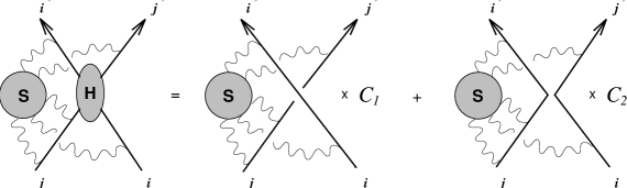
Figure 1: The general structure of the Feynman diagrams for the scattering of two Wilson lines at short transverse distances $z_{\perp}$. The soft gluons are factorized into two Wilson lines with a cross point at the origin. The coefficient functions $C_{1}$ and $C_{2}$ represent the hard gluons contribution.

Finally, substituting (12) and (13) into (11) we obtain the expression for the Wilson line (8) in the form of the operator product expansion

$$W^{i^{\prime}j^{\prime}}_{ij}(\gamma,\lambda^{2}z^{2})=C_{1}(\gamma,z^{2}\mu^{2}){\left({W_{1}}\right)}^{i^{\prime}j^{\prime}}_{ij}(\gamma,\mu^{2}/\lambda^{2})+C_{2}(\gamma,z^{2}\mu^{2}){\left({W_{2}}\right)}^{i^{\prime}j^{\prime}}_{ij}(\gamma,\mu^{2}/\lambda^{2})\equiv C\cdot W\,,$$ (14)

where the notation was introduced for the doublets

$$C=(C_{1},\ C_{2})\,,\qquad W={\left({{W_{1}\atop W_{2}}}\right)}\,.$$ (15)

To one-loop order, the calculation of the coefficient functions and the Wilson lines in the $\overline{\rm MS}$ scheme gives

$$(C_{1}-1)N_{c}=-C_{2}=-\frac{\alpha_{\rm s}}{\pi}{\left({i\pi\coth\gamma}\right)}\ln{\left({\mu|z_{\perp}|\mbox{e}^{-\gamma_{\sc e}}/2}\right)}+{\cal O}(\alpha_{\rm s}^{2})$$ (16)

with $\gamma_{\sc e}$ being the Euler constant and

$$W_{1}=\delta_{i^{\prime}i}\delta_{j^{\prime}j}-\frac{\alpha_{\rm s}}{\pi}\ln\frac{\mu}{\lambda} {\left({i\pi\coth\gamma}\right)}\left[-\frac{1}{N_{c}}\delta_{i^{\prime}i}\delta_{j^{\prime}j}+\delta_{i^{\prime}j}\delta_{j^{\prime}i}\right]+{\cal O}(\alpha_{\rm s}^{2})\,,$$

$$W_{2}=\delta_{i^{\prime}j}\delta_{j^{\prime}i}-\frac{\alpha_{\rm s}}{\pi}\ln\frac{\mu}{\lambda} \bigg{[}\hskip 8.53581pt\delta_{i^{\prime}i}\delta_{j^{\prime}j}{\left({\gamma\coth\gamma-i\pi\coth\gamma-1}\right)}$$

$$+\left.\delta_{i^{\prime}j}\delta_{j^{\prime}i}{\left({-N_{c}(\gamma\coth\gamma-1)+\frac{i\pi}{N_{c}}\coth\gamma}\right)}\right]+{\cal O}(\alpha_{\rm s}^{2})\,.$$

Substituting these expressions into (14) one reproduces the one-loop result (9) for $W^{i^{\prime}j^{\prime}}_{ij}$ renormalized in the $\overline{\rm MS}$ scheme.

We stress that the Wilson line operator in the l.h.s. of (14) is a nonlocal operator of the gauge fields both in the longitudinal and transverse planes. The relation (14) states that it can be expanded over two Wilson line operators which are still nonlocal in longitudinal plane but local in the transverse direction. We notice, however, that nonlocality of $W_{1}$ and $W_{2}$ in the longitudinal direction can be effectively eliminated if one uses the representation for the Wilson lines as correlators of local heavy quark fields in the effective heavy quark field theory [12].

3. Cross singularities of Wilson lines

The scattering amplitude (7) and the Wilson line (14) do not depend on an arbitrary factorization scale $\mu$ while the coefficient functions $C$ and the Wilson lines $W_{1,2}$ depend separately on $\mu$. In a full analogy with the standard OPE, the latter dependence can be found using the renormalization properties of the Wilson lines $W_{1}$ and $W_{2}$ defined in (13) and entering into the OPE expansion (14). These properties have been studied in details in past [13] without any relation to the high-energy scattering and they were found to depend on the choice of the integration contours $C$ and on the representation of the $SU(N_{c})$ group in which the Wilson lines are defined. The peculiar features of the Wilson lines $W_{1}$ and $W_{2}$ are that, first, they are defined in the fundamental (quark) representation and, second, the integration contours entering into their definitions cross each other at the origin. As a result, the Wilson lines $W_{1}$ and $W_{2}$ are mixed with each other under renormalization and their $\mu-$dependence is described by the following RG equation [13]

$${\left({\mu\frac{\partial}{\partial\mu}+\beta(g)\frac{\partial}{\partial g}+\Gamma_{\rm cross}(\gamma,\alpha_{\rm s})}\right)}W(\gamma,\mu^{2}/\lambda^{2})=0$$ (17)

with the doublet $W$ defined in (15). The evolution equation for the coefficient functions can be easily obtained from (14) and (17) using $\mu-$independence of the product $C\cdot W$. The equation (17) introduces into consideration a new object, a $2\times 2$ matrix of anomalous dimensions $\Gamma_{\rm cross}(\gamma,\alpha_{\rm s})$. As we will show below, this matrix governs the Regge behaviour of the quark-quark scattering amplitude in much the same way as the anomalous dimensions of local twist 2 operators define the evolution of the structure function of DIS.

The matrix of the cross anomalous dimensions $\Gamma_{\rm cross}(\gamma,\alpha_{\rm s})$ has the following interesting properties. It is gauge invariant and it depends only on the coupling constant and the cross angle $\gamma=\ln\frac{s}{m^{2}}$ but not on the color indices of the Wilson lines. The matrix $\Gamma_{\rm cross}(\gamma,\alpha_{\rm s})$ was calculated to two-loop order in QCD and its explicit expression as well as some general properties can be found in [14]. In application to high-energy scattering, it is of most importance to know the asymptotics of the matrix in the limit $\gamma=\ln\frac{s}{m^{2}}\gg 1$. In this limit, to all order in $\alpha_{\rm s}$, the different elements of the matrix have the following behaviour

$$\Gamma_{\rm cross}^{11}\sim\Gamma_{\rm cross}^{12}\sim\gamma^{0}\,,\qquad\Gamma_{\rm cross}^{21}\sim\Gamma_{\rm cross}^{22}\sim\gamma\,,$$ (18)

which would imply, in general, the asymptotics $\det\Gamma_{\rm cross}\sim\gamma$. However, the matrix elements have an interesting “fine structure”, due to which remarkable cancellation of the leading $\sim\gamma$ term occurs leading to $\det\Gamma_{\rm cross}\sim\gamma^{0}$ with $\mbox{tr\,}\Gamma_{\rm cross}\sim\gamma$. As a result, the eigenvalues $\Gamma_{\pm}$ of the matrix $\Gamma_{\rm cross}$ can be calculated as

$$\Gamma_{+}=\gamma\ \Gamma_{\rm cusp}(\alpha_{\rm s})+{\cal O}(\gamma^{0})\,,\qquad\Gamma_{-}={\cal O}(\gamma^{-1})\,,$$ (19)

with $\Gamma_{+}/\Gamma_{-}={\cal O}(\gamma^{2})$. Here, the leading coefficient $\Gamma_{\rm cusp}(\alpha_{\rm s})$ is closely related to the so-called “cusp” anomalous dimension and it is known to two-loop order as

$$\Gamma_{\rm cusp}(\alpha_{\rm s})=\frac{\alpha_{\rm s}}{\pi}N_{c}+{\left({\frac{\alpha_{\rm s}}{\pi}}\right)}^{2}N_{c}\left[N_{c}{\left({\frac{67}{36}-\frac{\pi^{2}}{12}}\right)}-n_{f}\frac{5}{18}\right]+{\cal O}(\alpha_{\rm s}^{3})$$ (20)

where $n_{f}$ is the number of light quark flavours.

The RG equation (17) was checked in [14] by performing the calculation of $W_{1}$ and $W_{2}$ to the order $\alpha_{\rm s}^{2}$. It was observed that the perturbative corrections to the Wilson lines vanish at $\mu=\lambda$

$$W_{1}(\gamma,1)=\delta_{i^{\prime}i}\delta_{j^{\prime}j}\,,\qquad W_{2}(\gamma,1)=\delta_{i^{\prime}j}\delta_{j^{\prime}i}\,.$$

Using this relation as a boundary condition, we solve the RG equation (17), obtain the expressions for the Wilson lines and substitute them into (14) to get

$$W^{i^{\prime}j^{\prime}}_{ij}(\gamma,\lambda^{2}z^{2})={\left({C_{1}(\gamma,\mu^{2}z^{2}),C_{1}(\gamma,\mu^{2}z^{2})}\right)}\ \cdot A(\gamma,\mu^{2}/\lambda^{2})\ \cdot{\left({{\delta_{i^{\prime}i}\delta_{j^{\prime}j}\atop\delta_{i^{\prime}j}\delta_{j^{\prime}i}}}\right)}\,,$$ (21)

where the notation was introduced for $2\times 2$ matrix

$$A(\gamma,\mu^{2}/\lambda^{2})={\cal T}\exp{\left({-\int_{\lambda}^{\mu}\frac{d\tau}{\tau}\Gamma_{\rm cross}(\gamma,\alpha_{\rm s}(\tau^{2}))}\right)}\,.$$ (22)

Here, the matrices $\Gamma_{\rm cross}(\gamma,\alpha_{\rm s}(\tau^{2}))$ do not commute for different values of $\tau$ and ${\cal T}$ orders them along the integration path. Except of the special cases [6, 5] (frozen coupling constant, one-loop order approximation for $\Gamma_{\rm cross}$), the evaluation of the matrix $A$ becomes extremely nontrivial.

4. Evolution equation

Substituting (21) into (7) one performs the Fourier transformation of the coefficient functions

$$\widetilde{C}_{1,\,2}(\gamma,q_{\perp}^{2}/\mu^{2})=i\frac{q_{\perp}^{2}}{4\pi}\int d^{2}z_{\perp}\ \mbox{e}^{iq_{\perp}\cdot z_{\perp}}C_{1,\,2}(\gamma,z_{\perp}^{2}\mu^{2})$$ (23)

and finally obtains the representation for the scattering amplitude in the form (5) with

$$(T_{1}(\gamma,q^{2}/\lambda^{2}),T_{2}(\gamma,q^{2}/\lambda^{2}))=\sigma_{0}\ (\widetilde{C}_{1}(\gamma,q^{2}/\mu^{2}),\widetilde{C}_{2}(\gamma,q^{2}/\mu^{2}))\,\cdot A(\gamma,\mu^{2}/\lambda^{2})\,,$$ (24)

where $\sigma_{0}=\frac{2\pi}{q_{\perp}^{2}}\frac{s}{m^{2}}$ and the matrix $A$ was defined in (22). In this relation, the dependence of the invariant scattering amplitudes $T_{1}$ and $T_{2}$ on the IR cutoff and on the transferred momentum $q^{2}$ is factorized into the matrix elements of the Wilson lines, $A$, and the coefficient functions $\widetilde{C}$, respectively. In the matrix notations, the doublet $\widetilde{C}$ and the matrix $A$ are renormalized multiplicatively and they satisfy the RG equations involving the anomalous dimension $\Gamma_{\rm cross}$. To one-loop order $\widetilde{C}_{1,2}$ can be obtained from (23) using (16) as

$$\widetilde{C}_{1}=-\frac{1}{N_{c}}\alpha_{\rm s}+{\cal O}(\alpha_{\rm s}^{2})\,,\qquad\widetilde{C}_{2}=\alpha_{\rm s}+{\cal O}(\alpha_{\rm s}^{2})\,.$$ (25)

As a function of the IR cutoff, the matrix (22) satisfies the relation $\lambda\frac{d}{d\lambda}A=A\Gamma_{\rm cross}$. Then, differentiating the both sides of (24) with respect to $\lambda$ we obtain the evolution equation for the scattering amplitudes as

$$\lambda\frac{d}{d\lambda}\ (T_{1},T_{2})=(T_{1},T_{2})\,\cdot\Gamma_{\rm cross}(\gamma,\alpha_{\rm s}(\lambda^{2}))\,.$$ (26)

This equation is a natural generalization of an analogous evolution equation for the Sudakov form factor in QCD [12]. In the latter case, all effects of soft gluon radiation are factorized into a single Wilson line and the dependence of the Sudakov form factor on the IR cutoff becomes in one-to-one correspondence with renormalization of the “cusp” singularities of the Wilson line. As a result, the Sudakov form factor satisfies the evolution equation similar to (26) with the matrix $\Gamma_{\rm cross}$ replaced by the “scalar” cusp anomalous dimension $\Gamma_{\rm cusp}$.

To identify the contribution of the Reggeon to the scattering amplitude (6) we exclude $T_{1}$ from the system (26) and obtain the evolution equation for $T_{2}$ as

$$T_{2}^{\prime\prime}+T_{2}^{\prime}\ f+T_{2}\ \varphi=0$$ (27)

with the coefficients $f$ and $\varphi$ defined as

$$f=-\mbox{tr\,}\Gamma_{\rm cross}-{\left({\ln\Gamma_{\rm cross}^{12}}\right)}^{\prime}\,,\qquad\varphi=\det\Gamma_{\rm cross}-{\left({\Gamma_{\rm cross}^{22}}\right)}^{\prime}+\Gamma_{\rm cross}^{22}{\left({\ln\Gamma_{\rm cross}^{12}}\right)}^{\prime}\,.$$ (28)

Here, the prime denotes the derivative $\frac{d}{d\ln\lambda}$ and the elements of $\Gamma_{\rm cross}(\gamma,\alpha_{\rm s})$ depend on $\lambda$ only through $\alpha_{\rm s}(\lambda^{2})$. We notice that the dependence on the energy $s$ enters into this equation via the matrix elements of the cross anomalous dimension. Using the asymptotics (18) and (19) we obtain the behavior of $f$ and $\varphi$ at large energy $s$, or equivalently at $\gamma\gg 1$, as

$$f=-\gamma\,\Gamma_{\rm cusp}(\alpha_{\rm s}(\lambda^{2}))+{\cal O}(\gamma^{0})\,,\qquad\varphi\sim\Gamma_{\rm cross}^{22}={\cal O}(\gamma)\,,$$ (29)

where the explicit expression for the leading term in $\varphi$ will not be important.

Let us first consider the evolution equation (27) is the LLA, $\alpha_{\rm s}\ln s\sim 1$ and $\alpha_{\rm s}\ll 1$. In this limit, one can neglect the $\lambda-$dependence of $\Gamma_{\rm cross}$ and omit in (28) the terms involving the derivatives of the matrix elements. The eigenvalues (19) of the matrix $\Gamma_{\rm cross}$ become

$$\Gamma_{+}^{\rm LLA}{=}\frac{\alpha_{\rm s}}{\pi}N_{c}\ln\frac{s}{m^{2}}\,,\qquad\quad\Gamma_{-}^{\rm LLA}{=}0$$

and using the identities $\det\Gamma_{\rm cross}=\Gamma_{+}\Gamma_{-}$ and $\mbox{tr\,}\Gamma_{\rm cross}=\Gamma_{+}+\Gamma_{-}$ one can obtain the solution of (27) in the LLA limit as

$$T_{2}^{\rm LLA}=\frac{2\pi\widetilde{C}_{2}}{q_{\perp}^{2}}\ {\left({\frac{s}{m^{2}}}\right)}^{1-\frac{\alpha_{\rm s}}{2\pi}N_{c}\ln\frac{q^{2}}{\lambda^{2}}}$$ (30)

with $\widetilde{C}_{2}\equiv\widetilde{C}_{2}(\gamma,1)$ being the integration constant independent of the IR cutoff. Comparing (30) with (6), (10) and (2) we find that the LLA solution of the evolution equation (27) correctly reproduces the one-loop correction to the Reggeon trajectory (2) provided that $\widetilde{C}_{2}=\alpha_{\rm s}$ in accordance with (25).

Let us now go beyond the LLA order and try to solve the evolution equation (27) assuming that the gluon is reggeized and the scattering amplitude $T_{2}$ has the Regge behaviour

$$T_{2}\sim{\left({\frac{s}{m^{2}}}\right)}^{1+\omega(q^{2})}\equiv\mbox{e}^{\gamma(1+\omega(q^{2}))}$$ (31)

with $\alpha(t)=1+\omega(t)$ being the Reggeon trajectory. To this end, we substitute the ansatz (31) into the evolution equation (27) and obtain the Ricatti equation for $\omega^{\prime}\equiv\frac{d}{d\ln\lambda}\omega$

$$\frac{1}{\gamma}\omega^{\prime\prime}+{\left({\omega^{\prime}}\right)}^{2}+\frac{f}{\gamma}\ \omega^{\prime}+\frac{\varphi}{\gamma^{2}}=0\,.$$

Using (29) together with $\omega={\cal O}(\gamma^{0})$, we notice that the first and the last terms in this equation are suppressed by a power of $\gamma$ and the third term is proportional to $\Gamma_{\rm cusp}$. Therefore in the leading $\gamma\to\infty$ limit the evolution equation is reduced to

$$\omega^{\prime}\equiv\lambda\frac{d\omega}{d\lambda}=\Gamma_{\rm cusp}(\alpha_{\rm s}(\lambda^{2}))$$ (32)

with $\omega$ being the function of $q^{2}/\lambda^{2}$ and $\alpha_{\rm s}(\lambda^{2})$. Integrating the evolution equation (32) we obtain the Reggeon trajectory as

$$\alpha_{\tiny{\hbox{{\rm I}\kern-0.99998pt\hbox{\rm R}}}}(t)-1=\omega(q_{\perp}^{2})=\Gamma_{\tiny{\hbox{{\rm I}\kern-0.99998pt\hbox{\rm R}}}}(\alpha_{\rm s}(q_{\perp}^{2}))-\frac{1}{2}\int_{\lambda^{2}}^{q_{\perp}^{2}}\frac{dk_{\perp}^{2}}{k_{\perp}^{2}}\Gamma_{\rm cusp}(\alpha_{\rm s}(k_{\perp}^{2}))\,,$$ (33)

or equivalently

$$\omega(q_{\perp}^{2})=\Gamma_{\tiny{\hbox{{\rm I}\kern-0.99998pt\hbox{\rm R}}}}(\alpha_{\rm s}(q_{\perp}^{2}))-\int_{\alpha_{\rm s}(\lambda^{2})}^{\alpha_{\rm s}(q_{\perp}^{2})}d\alpha_{\rm s}\frac{\Gamma_{\rm cusp}(\alpha_{\rm s})}{\beta(\alpha_{\rm s})}\,.$$ (34)

Here, the anomalous dimension $\Gamma_{\tiny{\hbox{{\rm I}\kern-0.99998pt\hbox{\rm R}}}}$ appears as the integration constant.

Using (33) one can expand the Reggeon trajectory as a double series in $\alpha_{\rm s}(\lambda^{2})$ and $L=\frac{1}{2}\ln\frac{q_{\perp}^{2}}{\lambda^{2}}$. The fact that $\omega(q_{\perp}^{2})$ satisfies the RG equation (32) imposes severe restrictions on this expansion. In particular, the leading term of the series has a form $(\alpha_{\rm s}L)^{n}$ with the coefficient in front proportional to a power of the $\beta-$function. This explains the origin of the $\alpha_{\rm s}^{2}L^{2}$ term and the cancellation of $\alpha_{\rm s}^{2}L^{3}$ term in (3). Moreover, one immediately identifies the coefficient $w_{2}$ in front of the $\alpha_{\rm s}^{2}L$ term in (3) as the 2-loop correction to the cusp anomalous dimension (20). As to remaining coefficient $w_{3}$ in (3), it provides the 2-loop correction to the anomalous dimension $\Gamma_{\tiny{\hbox{{\rm I}\kern-0.99998pt\hbox{\rm R}}}}$

$$\Gamma_{\tiny{\hbox{{\rm I}\kern-0.99998pt\hbox{\rm R}}}}={\left({\frac{\alpha_{\rm s}}{\pi}}\right)}^{2}N_{c}\left[{\left({\frac{101}{108}-\frac{1}{8}\zeta(3)}\right)}N_{c}-\frac{7}{54}n_{f}\right]+{\cal O}(\alpha_{\rm s}^{3})\,.$$ (35)

The following concluding remarks are in order. The solution of the evolution equation, (33) and (34), gives the expression for the Reggeon trajectory in terms of three functions of the coupling constant: the $\beta-$function, the cusp anomalous dimension, $\Gamma_{\rm cusp}$, and the anomalous dimension $\Gamma_{\tiny{\hbox{{\rm I}\kern-0.99998pt\hbox{\rm R}}}}$. The universality of the Reggeon trajectory implies that the functions should not depend on the scattered particles. This is certainly true for the $\beta-$function but it is not obvious for $\Gamma_{\rm cusp}$ and $\Gamma_{\tiny{\hbox{{\rm I}\kern-0.99998pt\hbox{\rm R}}}}$. Replacing the scattering particles, one has to change correspondingly the representation of the $SU(N_{c})$ group, in which the Wilson lines are defined in (7). The renormalization properties of the Wilson lines will also be changed and, in particular, the matrix of the cross anomalous dimensions will have a different dimension. However, in the high-energy limit, $\gamma\to\infty$, only the largest eigenvalue of the matrix will survive. It will coincide with $\Gamma_{+}$ and will lead to the evolution equation (32).

Since the anomalous dimensions $\Gamma_{\rm cusp}$ and $\Gamma_{\tiny{\hbox{{\rm I}\kern-0.99998pt\hbox{\rm R}}}}$ arose from the analysis of the quark-quark scattering amplitude, one would naively expect that they should be defined in the quark representation. However, their explicit expressions, (20) and (35), do not contain the corresponding quadratic Casimir operator $C_{F}$ and, moreover, $\Gamma_{\rm cusp}$ coincides with the expression (20) for the cusp anomalous dimension in the adjoint representation.

The anomalous dimensions $\Gamma_{\rm cusp}$ and $\Gamma_{\tiny{\hbox{{\rm I}\kern-0.99998pt\hbox{\rm R}}}}$ appeared as peculiar properties of the Wilson lines describing the high-energy quark–quark scattering. We would like to notice that the Wilson lines themselves exhibit interesting universality properties. Calculating perturbative corrections to Wilson lines describing IR asymptotics of different hard processes in different kinematics one obtains expressions similar to (3) and (33) with the same “leading” anomalous dimension $\Gamma_{\rm cusp}$ and different $\Gamma_{\tiny{\hbox{{\rm I}\kern-0.99998pt\hbox{\rm R}}}}$. As an example, one considers the 2-loop calculation of the light-like rectangular Wilson line $W_{\Box}$ in the adjoint representation of the $SU(N_{c})$ describing the IR asymptotics of the gluon string operator in QCD [16]. Due to additional light-like singularities, the perturbative ${\cal O}(\alpha_{\rm s}^{2})$ expansion of $\ln W_{\Box}$ starts with $\alpha_{\rm s}^{2}L^{3}$ term with $L$ being the IR logarithm. In a complete analogy with (3), the coefficients in front of the leading and next-to-leading terms are proportional to the $\beta$ function and $\Gamma_{\rm cusp}$, respectively, while the next-to-next-to-leading coefficient is ${\left({\frac{101}{54}-\frac{7}{4}\zeta(3)}\right)}N_{c}-\frac{7}{27}n_{f}\,.$ Remarkably enough, this expression coincides with $2w_{3}$ defined in (3) up to $\zeta(3)-$term. We believe that the agreement is not incidental.

Our calculation of the scattering amplitude was entirely perturbative and it relied on the fact that the transferred momentum $q_{\perp}^{2}$ and the IR cutoff have been chosen in (4) to be large enough for the perturbative expansion in (33) to be meaningful. Once $q_{\perp}^{2}$ and $\lambda^{2}$ are decreasing toward $\Lambda_{\sc qcd}^{2}$ one should expect the emergence of nonperturbative corrections to the Reggeon trajectory. Their general structure can be predicted by analysing ambiguities of the perturbative series related to the contribution of the IR renormalons [17, 18, 19]. Using the nonperturbative definition (7) of the scattering amplitude as Fourier transformed Wilson line expectation value, one can identify the leading IR renormalon contribution to the scattering amplitude and to the Reggeon trajectory [17].

The Reggeon trajectory (33) provides an additive correction to the BFKL kernel. In the BFKL Pomeron, built from two Reggeons, IR divergences of the Reggeon trajectory, described by the last term in the r.h.s. of (33), are effectively cancelled with the contribution to the BFKL kernel due to Reggeon-Reggeon interaction. It is the finite part left after the cancellation which provides the correction to the BFKL Pomeron. Similar situation occurs in the Drell-Yan process, in which the Sudakov form factor plays a role of the gluon Regge trajectory. In this case, large finite perturbative corrections to the cross section can be resummed to all orders [20] and the analysis [21] similar to the one performed in the previous sections allows to establish their intrinsic connection to the cusp singularities of the Wilson lines. This suggests that there should exist a relation between the nonleading corrections to the BFKL Pomeron and certain properties of the Wilson lines (see e.g. [22]).

Acknowledgements

One of us (G.P.K.) is most grateful to V.N. Gribov for stimulating discussions.

References

• [1] V.N. Gribov, Sov. Phys. JETP 26 (1968) 414; Nucl. Phys. B106 (1976) 189.
• [2] V.S. Fadin, E.A. Kuraev and L.N. Lipatov, Phys. Lett. B60 (1975) 50; Sov. Phys. JETP 44 (1976) 443; 45 (1977) 199;
Ya.Ya. Balitsky and L.N. Lipatov, Sov. J. Nucl. Phys. 28 (1978) 822.
• [3] J.C. Collins, D.E. Soper and G. Sterman, in Perturbative QCD, ed. A.H. Mueller, World Scientific Publ., 1989.
• [4] J. Botts and G. Sterman, Nucl. Phys. B325 (1989) 62; Phys. Lett. B224 (1989) 201.
• [5] G.P. Korchemsky, Phys. Lett. B325 (1994) 459.
• [6] M.G. Sotiropoulos and G. Sterman, Nucl. Phys. B425 (1994) 489; B419 (1994) 59.
• [7] L.N. Lipatov, Nucl. Phys. B309 (1988) 379.
• [8] V.S. Fadin and L.N. Lipatov, JETP Lett. 49 (1989) 352; Sov. J. Nucl. Phys. 50 (1989) 712; preprint DESY-96-020, Feb 1996; [hep-ph/9602287].
• [9] V.S. Fadin, R. Fiore and M.I. Kotsky, Phys. Lett. B359 (1995) 181;
V.S. Fadin, R. Fiore and A. Quartarolo, Phys. Rev. D53 (1996) 2729.
• [10] V.S. Fadin, R. Fiore and M.I. Kotsky, preprint BUDKER-INP/96-35, May 1996; [hep-ph/9605357].
• [11] E. Verlinde and H. Verlinde, preprint PUPT-1319, Feb 1993; [hep-th/9302104].
• [12] G.P. Korchemsky and A.V. Radyushkin, Phys. Lett. B171 (1986) 459; B279 (1992) 359.
• [13] R.A. Brandt, F. Neri and M.-A. Sato, Phys. Rev. D24 (1981) 879.
• [14] I.A. Korchemskaya and G.P. Korchemsky, Nucl. Phys. B437 (1995) 127.
• [15] M. Beneke and V.M. Braun, Nucl. Phys. B454 (1995) 253.
• [16] I.A. Korchemskaya and G.P. Korchemsky, Phys. Lett. B287 (1992) 169.
• [17] I.A. Korchemskaya, preprint ITP-SB-95-19, May 1995; [hep-ph/9506402].
• [18] E.M. Levin, Nucl. Phys. B453 (1995) 303.
• [19] K.D. Anderson, D.A. Ross and M.G. Sotiropoulos, preprint SHEP-96-06, Feb 1996; [hep-ph/9602275].
• [20] G. Sterman, Nucl. Phys. B281 (1987) 310;
S. Catani and L. Trentadue, Nucl. Phys. B327 (1989) 323; B353 (1991) 183.
• [21] G.P. Korchemsky and G. Marchesini, Phys. Lett. B313 (1993) 433.
• [22] I. Balitsky, Nucl. Phys. B463 (1996) 99.